Short Circuits in Thermally Ionized Plasmas: A Mechanism for Intermittent Heating of Protoplanetary Disks

Abstract

Many astrophysical systems of interest, including protoplanetary accretion disks, are made of turbulent magnetized gas with near solar metallicity. Thermal ionization of alkali metals in such gas exceeds non-thermal ionization when temperatures climb above roughly 1000 K. As a result, the conductivity, proportional to the ionization fraction, gains a strong, positive dependence on temperature. In this paper, we demonstrate that this relation between the temperature and the conductivity triggers an exponential instability that acts similarly to an electrical short, where the increased conductivity concentrates the current and locally increases the Ohmic heating. This contrasts with the resistivity increase expected in an ideal magnetic reconnection region. The instability acts to focus narrow current sheets into even narrower sheets with far higher currents and temparatures. We lay out the basic principles of this behavior in this paper using protoplanetary disks as our example host system, motivated by observations of chondritic meteorites and their ancestors, dust grains in protoplanetary disks, that reveal the existence of strong, frequent heating events that this instability could explain.

1. Introduction

In this paper, we describe an exponential instability that acts to narrow and strengthen current sheets in partially ionized gas with a resistivity inversely dependent on temperature. While the physics that we describe pertains to any magnetized system with both current sheets and a conductivity that increases strongly enough with temperature, this problem arises specifically in the context of protoplanetary disks, where the formation of high-temperature minerals such as chondrules and crystalline silicates suggests strong, intermittent heating events.

As the local temperature in such a disk climbs above $\sim 1000$ K, the dominant source of free electrons becomes the thermal ionization of alkaline metals. These temperatures are still well below the ionization energy, so the argument of the exponential in the Boltzmann term is quite small; thus the ionization fraction $x_{e}=n_{e}/n_{n}$ depends steeply on temperature. We have found that this results in startling new behavior with positive temperature fluctuations increasing conductivity, concentrating current sheets, and positively feeding back on the temperature through enhanced local Ohmic heating.

This is quite different from classical reconnection, with electrical short circuits effectively forming in these regions. This effect is the opposite of the more commonly assumed anomalous resistivity that increases in the reconnection region (Krall & Liewer, 1971; Sato & Hayashi, 1979; Yamada et al., 2010). (Classical reconnection was applied to disks using general energetic arguments by King & Pringle 2010.) While our mechanism narrows current sheets, similarly to ambipolar diffusion (Brandenburg & Zweibel, 1994), the mechanism is Ohmic resistivity rather than a drift of the charge carriers relative to the neutral gas. Our mechanism is also different from previous work on partially ionized reconnection because that focused on the transition to the collisionless regime (Malyshkin & Zweibel, 2011; Zweibel et al., 2011).

Observations of protostellar disks have revealed their integrated properties, including masses (Beckwith & Sargent, 1993) and accretion rates (Hartmann, 1998). Compositional gradients in the dust (Van Boekel et al., 2004) can be detected, as well as the difference between predominantly amorphous and crystalline mineral structures at different radii (Waelkens et al., 1996; Malfait et al., 1998). The observed presence of crystalline minerals at large radii (Sargent et al., 2009) suggests the need for a heating mechanism active in the disk far from the parent star. Meanwhile, we have direct evidence of conditions in the protosolar disk. Laboratory measurements of textural, mineralogical, chemical, and isotopic properties of meteoritic chondrules and calcium-aluminum rich inclusions, as well as related high-temperature materials in comet samples (Brownlee et al., 2006; Zolensky et al., 2006; Nakamura et al., 2008; Simon et al., 2008), give strong constraints on their local formation history and environment. They represent melts condensed and cooled from temperatures of 1500–1800 K at rates of around 100–1000 K/hour (Radomsky and Hewins, 1990; Lofgren and Lanier, 1990; Connolly et al., 1998; Scott & Krot, 2005; Ebel, 2006): far faster than disk dynamical timescales, but far slower than the free-space cooling time of millimeter sized objects. The source of these processed materials in unclear. While there is a vast reservoir of gravitational potential energy in the disk, tapping it through an accretion flow to create hot regions of finite size, as appears to be needed, is non-trivial.

The primary source of angular momentum transport in protoplanetary disks appears to be the conversion of orbital kinetic energy into magnetic energy through the magnetorotational instability (MRI; Velikhov, 1959; Chandrasekhar, 1961; Balbus & Hawley, 1991, 1998), with gravitational instability playing a larger role at earlier times (e.g Lodato & Rice, 2004). The ionization structure of the disk midplane may introduce a magnetically dead zone at some radii and periods of disk history (Gammie, 1996), with reduced though non-zero turbulent viscosity (Fleming and Stone, 2003; Oishi & Mac Low, 2009). Its exact structure and history remains controversial (Glassgold et al., 1997; Sano et al., 2000; Ilgner and Nelson, 2006; Umebayashi & Nakano, 2009; Turner & Drake, 2009).

MRI draws on the huge amount of energy contained in the differential rotation of the disk to drive magnetohydrodynamical (MHD) turbulence. The turbulence will dissipate that energy into heat. However, the heating will occur intermittently, not uniformly. MHD turbulence forms current sheets (Parker, 1972, 1994; Cowley et al., 1997) that dissipate energy at far greater than the average rate, and can provide locations for magnetic reconnection to occur. Romanova (2011) noted in passing the volume filling nature of this mechanism (also see Romanova et al., 2011). Hirose & Turner (2011) used a moderate resolution simulation to demonstrate that such current sheets forming in the atmosphere above a dead zone can locally heat gas well above the radiative equilibrium temperature. Those calculations, along with preliminary work of our own McNally (2012a); McNally et al. (2012b) suggests that such current sheets may well heat the gas up to temperatures sufficiently high for the instability described here to set in.

This is hardly the first suggestion that electromagnetic fields can drastically alter the temperature profile in a protoplanetary disk. Levy & Araki (1989) examined reconnection heating in disks as a chondrule formation mechanism. However, they worked before the nature of the turbulence driving angular momentum transport was understood. Therefore, they reasoned by analogy to the Sun that a stratified, convective, magnetized flow would drive reconnection in the low density region above it. Thus, they only considered coronal heating many scale heights above the surface of the disk. However, we now understand that the turbulence in the disk is probably not convective but rather driven by the differential rotation acting through the field, so that intermittent dissipation will occur throughout the disk. The short-circuit instability is in many ways similar to lightning (Whipple, 1966; Horanyi et al., 1995; Pilipp et al., 1998; Desch & Cuzzi, 2000; Muranushi, 2010; Muranushi et al., 2012): a rapid local increase in the ionization fraction leads to high currents and a dramatic release of energy. However, there are significant differences in that the increase in ionization is thermal rather than due to electric fields strong enough to directly induce ionization breakdown. Further, the dynamo magnetic fields act as a current source rather than a voltage source. Electrical-short like behavior is only possible due to the residual current that flows in the low temperature regions around the instability, maintaining a non-trivial Ohmic electric field (see Section 2.2). This allows us to bypass the need to generate. electric fields strong enough to directly ionize the gas, which is a non-trivial challenge to lightning models. Another related proposed mechanism is melting of charged dust by acceleration through standard reconnection regions (Lazerson, 2010).

In this paper, we lay out the basic principles of this novel behavior, and explore the implications for heating in dusty protoplanetary disks in more detail in a companion paper McNally et al. (2012b, hereafter Paper II). Closely related behavior in planetary atmospheres was found by Menou (2012), who called it the thermo-resistive instability; though that term was also used by Price et al. (2012) for a system where the resistivity increases with temperature.

In Sect. 2 we describe the physical principles at play. In Sect. 3 we lay out a numerical approach to modeling this behavior, whose results are described in Sect. 4, and discussed in Sect. 5.

2. Temperature dependent resistivity

2.1. Spatially-varying resistivity

Consider the induction equation in the presence of Ohmic resistivity $\eta$

$$\frac{\partial{\mbox{\boldmath$B$}{}}}{\partial\hskip 0.59998pt{t}}={\bm{\nabla}}\times\left(\mbox{\boldmath$U$}{}\times\mbox{\boldmath$B$}{}-\eta\mbox{\boldmath$J$}{}\right),$$ (1)

where $B$ is the magnetic flux, $J$ the current, $\eta$ the resistivity, and $t$ time. If the resistivity is spatially uniform as normally assumed, then the resistive term can be rewritten:

$$\frac{\partial{\mbox{\boldmath$B$}{}}}{\partial\hskip 0.59998pt{t}}={\bm{\nabla}}\times\left(\mbox{\boldmath$U$}{}\times\mbox{\boldmath$B$}{}\right)+\eta\mbox{\boldmath$\nabla$}{}^{2}\mbox{\boldmath$B$}{},$$ (2)

where the effect of the resistivity is to diffuse the magnetic field. However, if the resistivity varies spatially, we must consider its spatial derivative:

$$\frac{\partial{\mbox{\boldmath$B$}{}}}{\partial\hskip 0.59998pt{t}}={\bm{\nabla}}\times\left(\mbox{\boldmath$U$}{}\times\mbox{\boldmath$B$}{}\right)+\eta\mbox{\boldmath$\nabla$}{}^{2}\mbox{\boldmath$B$}{}-\left(\mbox{\boldmath$\nabla$}{}\eta\right)\times\mbox{\boldmath$J$}{}.$$ (3)

If the resistivity shows strong spatial variation, the final term in Equation (3) can dominate over the diffusive one. In the limit of a one-dimensional system, varying along ${\bm{x}}$ with the magnetic field pointing along ${\bm{y}}$, we have

$$\frac{\partial B_{y}}{\partial t}=-\partial_{x}\left[v_{x}B_{y}\right]+\eta\partial_{x}^{2}B_{y}+\partial_{x}\eta\partial_{x}B_{y}.$$ (4)

If the $\partial_{x}\eta\partial_{x}B_{y}$ term is dominant over the diffusive term $\eta\partial_{x}^{2}B_{y}$, the Ohmic resistivity can act to steepen, rather than broaden, magnetic field gradients.

This consideration of the spatial variation of the resistivity comes into full focus if the resistivity drops steeply with temperature, which can occur in a mostly neutral plasma in temperature ranges where one or more species is being thermally ionized. In this case, a local positive temperature perturbation that increases ionization will drive a positive current perturbation, which can in turn result in an increase in the local Ohmic heating.

2.2. Steady State

The base problem is one common to elementary electrical circuits: electrical shorts, albeit in the current driven regime. To put this on a quantitative basis, let us begin by considering a base steady-state one-dimensional system of length $L$, aligned with the $x$-axis and centered at $x=0$, with magnetic structure given by

$$B_{y}|_{\pm L/2}=\pm B_{0}/2$$ (5)

$$J_{z}=\partial B_{y}/\partial x$$ (6)

$$\partial B_{y}/\partial t=\partial_{x}\left(\eta J_{z}\right)=0.$$ (7)

Under the assumption of uniform $\eta=\eta_{0}$ we have simply $J_{z}=B_{0}/L\equiv J_{0}$. Note that we have assumed that the velocity is $u_{x}=0$.

We now perturb the system, decreasing the resistivity to $\eta=\eta^{\prime}=\overline{\eta}\,\eta_{0}$ in a region of width $\Delta L=\overline{\delta}L$, centered at $x=0$. Equations (5) – (7) then require

$$\left(1-\overline{\delta}\right)J_{1}+\overline{\delta}J_{1}^{\prime}=J_{0}$$ (8)

$$J_{1}=\overline{\eta}J_{1}^{\prime},$$ (9)

from which we can derive

$$J_{1}^{\prime}=\left[\overline{\delta}+(1-\overline{\delta})\overline{\eta}\right]^{-1}J_{0},$$ (10)

where $J_{1}$ is the value of $J_{z}$ in the region with $\eta=\eta_{0}$ and $J_{1}^{\prime}$ is the value of $J_{z}$ in the region with $\eta=\eta^{\prime}$. As long as $\overline{\eta}<1$, $J_{1}^{\prime}>J_{0}$, which is quite natural as current will preferentially flow in regions of low resistivity.

More interesting is the Ohmic dissipation. The dissipation in the perturbed region $\eta^{\prime}J_{1}^{\prime 2}$ always exceeds that in the unperturbed region, as the electric fields in the two regions are equal by the requirement of a steady state. It also exceeds the dissipation in the base state $\eta_{0}J_{0}^{2}$ if

$$\overline{\eta}^{1/2}>\frac{\overline{\delta}}{1-\overline{\delta}}.$$ (11)

This implies that even small decreases in the resistivity result in increased heating (effectively an electrical short) as long as $\overline{\delta}<1/2$. This size limitation is required to maintain sufficient residual current in the non-perturbed region that the electric field resistively generated there can be the effective voltage source for the short.

In a partially ionized medium where the resistivity decreases with temperature because thermal ionization produces increased charge carrier density, one would expect the perturbed region to continue heating, reducing its resistivity further. Interestingly, this effect actually will reduce the total energy dissipated: the total current is constant, and we are reducing the resistivity of the medium the current flows through. While this effect generates local hot spots, it also decreases the total rate at which magnetic energy is dissipated into heat.

2.3. Instability Analysis

Section 2.2 gives a qualitative picture of a system that seems likely to experience an instability that would lead to an ever narrowing current sheet with increasing temperature and local heating. A real system will not be so idealized of course. We can explore the instability conditions quantitatively by performing a linear stability analysis on a slightly less simplified one-dimensional model. We assume an incompressible fluid that cools (presumably radiatively) to a background bath temperature $T_{b}$ in a time $t_{b}$. The equations are then

$$\frac{\partial B_{y}}{\partial t}=-\partial_{x}\left[-\eta\partial_{x}B_{y}\right],$$ (12)

$$\frac{\partial T}{\partial t}=-\frac{T-T_{b}}{t_{b}}+\frac{T_{0}}{t_{h}}\frac{\eta\left(\partial_{x}B_{y}\right)^{2}}{\eta_{0}J_{0}^{2}},$$ (13)

where the Ohmic heating time is $t_{h}$. The Ohmic heating term is normalized at the reference temperature $T_{0}$ by the Ohmic heating with $\eta=\eta_{0}$ and $J=J_{0}$. More exactly, we define the heating time

$$t_{h}=\frac{4\pi n_{n}k_{B}T_{0}}{\left(\gamma-1\right)\eta_{0}J_{0}^{2}},$$ (14)

where the factor of $4\pi$ comes from our use of cgs electromagnetic units, $n_{n}$ is the neutral number density and we assume a low ionization fraction. We track the temperature dependence of the resistivity through the general equation

$$\left.\frac{\partial\eta}{\partial T}\right|_{T_{0}}=-\frac{\eta_{0}}{T_{1}},$$ (15)

where $T_{1}$ parameterizes the strength of the temperature gradient of $\eta$. This also allows us to define the heating time of the resistivity $t_{\eta^{\prime}}$ through

$$t_{\eta^{\prime}}\equiv\eta_{0}\left|\frac{T_{0}}{t_{h}}\left.\frac{\partial\eta}{\partial T}\right|_{T_{0}}\right|^{-1}=\frac{T_{1}}{T_{0}}t_{h}.$$ (16)

In a dominantly neutral medium in LTE, the Saha equation is a simple approximation to the thermal ionization behavior, and the resistivity is dominated by the ionization fraction (see Equations 32 and 33 for more detail). In that case, considering only the exponential term in Equation 33 for analytic simplicity, Equation (15) becomes

$$\left.\frac{\partial\eta}{\partial T}\right|_{T_{0}}\simeq\left(-\frac{T_{i}}{T_{0}^{2}}\right)\eta_{0},$$ (17)

where $T_{i}$ is the temperature associated with first ionization . With $T_{i}=2.5188\times 10^{4}$ K, the ionization temperature of potassium, this approximates the ionization behavior of protoplanetary disks at $T\sim 1000$ K, as potassium has a low first ionization energy ($k_{B}T_{i}$) and sufficient abundances (Fromang et al., 2002). In this case, Equation (16) becomes

$$t_{\eta^{\prime}}=\frac{T_{0}}{T_{i}}t_{h}.$$ (18)

With these approximations and definitions, we can derive the dispersion relation for a perturbation of the form $e^{ikx+\lambda t}$ applied to a base state with

$$B_{y}(x)=J_{0}x$$ (19)

$$T(x)=T_{0}.$$ (20)

The linearized equations for the perturbations are

$$\lambda\triangle B=\frac{\eta_{0}J_{0}ik\triangle T}{T_{1}}-\eta_{0}k^{2}\triangle B$$ (21)

$$\lambda\triangle T=-\frac{\triangle T}{t_{b}}-\frac{2\triangle T}{t_{\eta^{\prime}}}+2\frac{T_{0}}{t_{h}}\frac{ik\triangle B}{J_{0}}.$$ (22)

Solving Equations (21) and (22) we find

$$\lambda^{2}+\lambda\left[\frac{1}{t_{r}}+\frac{1}{t_{b}}+\frac{1}{t_{\eta^{\prime}}}\right]+\frac{1}{t_{r}}\left[\frac{1}{t_{b}}-\frac{1}{t_{\eta^{\prime}}}\right]=0,$$ (23)

where $t_{r}\equiv k^{2}/\eta_{0}$ is the resistive time of the perturbation. As $t_{r},t_{\eta^{\prime}}$ and $t_{b}$ are all positive, it follows that the perturbation can exhibit exponential growth ($\lambda>0$) if the constant term in Equation (23) is negative, i.e. if

$$t_{\eta^{\prime}}<t_{b},$$ (24)

which condition is independent of $t_{r}$, unlike the usual situation for reconnection. While in the following section we will assume a resistivity profile that gives Equation (17), the existence of the instability requires only a strong enough gradient of the temperature dependence of $\eta$ (as measured through $T_{1}$ and $t_{\eta^{\prime}}$).

The independence of Equation (24) on $t_{r}$ arises in part because the resistivity plays an equal role in in the resistive time $t_{r}$ and the Ohmic heating time $t_{h}$ and in part because the magnetic field transport is mediated purely through resistive effects in the imposed absence of velocity. The steepening of magnetic field gradients through this instability and standard resistive spreading of magnetic fields occur through the same resistivity operator. We emphasize this point: the transport of magnetic fields into the dissipation region is resistive in nature, rather than advective. Accordingly, this mechanism does not immediately struggle with the problem of exhaust that has bedeviled attempts to understand observed fast reconnection in the solar corona and elsewhere.

The above analysis is a significant simplification of actual physical systems even beyond its one-dimensional nature. In particular, we note that in a physical reconnection region, the background current is not constant in time, and would be expected to decay resistively until the unstable modes have had time to grow. This occurs through the diffusive term in Equation (4) applied to the background current, which have been set to $0$ by our choice of background state, but which will not be negligible in general.

As we will see, the assumption of a single physical length scale imposed in the above analysis also breaks down in practice, with the high temperature region narrowing over time in the non-linear regime. Further, MRI-active protoplanetary disks are compressible and expected to have minimal plasma $\beta\sim 1$–$10$. The simulations described in the next section include these complications by implementing terms such as the Lorentz force, which acts to compress a current sheet, and adiabatic heating and cooling. Finally, we note that our analysis of the current sheet has been done along the shortest dimension, and that the current sheet will be much larger in the perpendicular, neglected dimensions. Because of this, the approximation of cooling to a bath temperature is a noteworthy oversimplification, and any cooling may act to expand the high temperature regions by radiative heating of the surroundings, as treated in more detail in Paper II.

3. Equations and numerical methods

3.1. Numerical methods

To model the dramatic behavior suggested by the linear analysis, we have written a one dimensional code using sixth order finite differences on a logarithmic grid. We use implicit time integration with the CVODE package (Hindmarsh et al., 2005). This allows us to follow the large, spatially limited variations in the resistivity. The logarithmically spaced grid allows us to push the boundaries towards infinity while retaining resolution in the center of the current sheet. The number of grid points used in the simulations reported here varies from 500 to 1000. Only the right half of the domain is included ($x>0$) and a symmetrical inner boundary condition is used.

3.2. Equations

We solve the MHD fluid equations in 1.5 dimensions, including $x$-gradients and $y$-components of vectors, with the one non-ideal term being the Ohmic resistivity. We use a somewhat more exact model of thermal ionization dominated by potassium. Although the linear analysis presented in Section 2.3 considered cooling, for this model we neglect cooling terms, deferring that additional complexity to Paper II. We use cgs units: magnetic field in Gauss and density in $\mathrm{g}/\mathrm{cm}^{-3}$.

With these approximations, the MHD equations become

$$\frac{\partial\rho}{\partial t}=-\partial_{x}\left(\rho v_{x}\right),$$ (25)

$$\frac{\partial v_{x}}{\partial t}=-v_{x}\partial_{x}v_{x}-\frac{1}{\rho}\partial_{x}P-\frac{1}{8\pi\rho}\partial_{x}B_{y}^{2}+\partial_{x}\zeta_{S}\partial_{x}v_{x},$$ (26)

$$\frac{\partial B_{y}}{\partial t}=-\partial_{x}\left[v_{x}B_{y}-\eta(x)\partial_{x}B_{y}\right],$$ (27)

$$\frac{\partial T}{\partial t}=-\partial_{x}\left(Tv_{x}\right)-c_{T}Pv_{x}$$

$$\quad\quad\quad\quad+\frac{c_{T}\eta}{4\pi\rho}\left(\partial_{x}B_{y}\right)^{2}+c_{T}\zeta_{S}\left(\partial_{x}v_{x}\right)^{2},$$ (28)

where $\zeta_{S}$ is a shock viscosity included for stability. The shock viscosity $\zeta_{s}$ is given by

$$\zeta_{s}=C_{s}\max(-\partial_{x}v_{x}\Delta x^{2})_{+}$$ (29)

where the constant $C_{s}$ is taken as $10$, $\max()_{+}$ denotes taking the maximum positive value over five grid points or zero otherwise, and $\Delta x$ is the grid spacing. The equation of state is that of an ideal gas and $c_{T}$ is the conversion factor between temperature and energy:

$$P=n_{n}k_{B}T,$$ (30)

$$c_{T}\equiv\frac{\left(\gamma-1\right)m_{n}}{k_{B}},$$ (31)

where we use $\gamma=7/5$, $n_{n}$ is the neutral number density (assumed to dominate) and $m_{n}$ is the neutral molecular mass. The resistivity associated with a dominantly neutral gas is given by Balbus & Terquem (2001)

$$\eta=234T^{1/2}x_{e}^{-1}\rm{cm}^{2}/\rm{s}$$ (32)

and the ionization fraction $x_{e}\equiv n_{e}/n_{n}$, under the assumption that the species being ionized is predominantly neutral and thermally ionized, becomes

$$x_{e}=8.7\times 10^{9}~{}a^{1/2}\left(\frac{n_{n}}{1~{}\mathrm{cm}^{-3}}\right)^{-1/2} \left(\frac{T}{10^{3}\rm{K}}\right)^{3/4}$$

$$\times\exp\left(-\frac{T_{i}}{T}\right).$$ (33)

where $a$ is the fraction of the ionizing species to the total neutral population. In our canonical model, we consider only the thermal ionization of potassium (Fromang et al., 2002).

At the densities $\rho\sim 10^{-9}$g/cm³, mean molecular mass $\mu=2.33$ and potassium fraction $a=10^{-7}$ of our canonical model, this equation breaks down at $T\gtrsim 1600\,$K when the potassium is significantly ionized. At higher temperatures in protoplanetary disks, other metals will also begin to contribute to the free electrons. At lower temperatures, below $T\sim 1000\,$K, the ionization fraction from thermal processes becomes so low that in any astrophysical system some non-thermal ionization source, such as ionizing stellar radiation or radionuclide decay, will dominate over thermal ionization. Even if they did not, the physical length scales required to achieve any MHD action in the presence of so high a resistivity become absurd. While for physical purposes, Equation (33) only applies in the temperature range $1000\,$K–$1600\,$K, we will consider evolution at starting temperatures of $500\,$K and $2000\,$K to help test predictions about the strength of the gradient of the resistivity with respect to temperature.

3.2.1 Initial and boundary conditions

We consider initial conditions with $v_{x}=0$, $\rho_{0}=10^{-9}$ g cm^-3, $a=10^{-7}$ and

$$B_{y}(x)=B_{0}^{\prime}\tanh(x/\ell_{0}),$$ (34)

which reproduces the magnetic field of a Harris (1962) current sheet. The density and potassium abundances are inspired by conditions in the midplanes of protoplanetary disks with active MRI (Boss, 1996; Sano et al., 2000). We denote the initial conditions at the box edge with the subscript $0$, and use box widths large enough compared to $\ell_{0}$ that $B_{0}$ and $B_{0}^{\prime}$ are functionally identical. The density and temperature are then set to counterbalance the Lorentz force in the center assuming an adiabatic compression. $B_{0}$ is a control parameter that sets the total magnetic energy in the simulation. As we are interested in the ability of the magnetic field to heat the gas, instead of labeling runs with $B_{0}$, we label them with the plasma beta: the ratio of thermal to magnetic pressure

$$\beta_{0}=8\pi\rho_{0}k_{B}T_{0}/(\mu m_{p}B_{0}^{2}).$$ (35)

A value of $\beta_{0}\sim 1$ signifies an initial magnetic field energy that could raise the temperature throughout the box by $\sim 50\%$ if converted directly to heat. The conversion is, however, localized in our models resulting in intermittent regions with substantially higher temperatures.

We list our control parameters in Table 1. A characteristic driving scale for turbulence in the inner portion of a protoplanetary disk would be $L\sim 5\times 10^{10}$ cm, estimated at $1$ AU for a Shakura-Sunyaev $\alpha=10^{-2}$ (Shakura & Sunyaev, 1973). The accretion luminosity and the irradiation from the central star are inadequate to raise the volume averaged temperatures to $T\sim 1000$ K at that position for prolonged periods. Still, temperature spikes, through magnetic reconnection, shocks or accretion events could all contribute to the temperature structure, leaving $1$ AU a convenient scale: just far enough from the central star that temperature excursions are unlikely to hit the $1000$ K threshold. Observations of protoplanetary disks also show an inner wall where dust is sublimated near $1500$ K, so the existence of regions where the temperature exceeds $1000$ K is not in doubt (e.g. Dullemond & Monnier, 2010).

The resistive time scales that we derive drop quickly with increasing temperature up to 1500 K. This leads to the concern that resistive diffusion might destroy current sheets before the ionization instability can grow. However, the growth time of the instability depends linearly on the resistive time (see Equation (44)), so that as the resistive time drops, the instability grows proportionally faster. The growth time, when measured in terms of the resistive time, does increase with the plasma $\beta$ (see discussion in Sect. 4.1, where $t_{c}$ is a growth time estimate). Values of the plasma $\beta$ of the order of 3–10 have been reported to occur above the midplane in moderate resolution models of MRI-active disks (Flock et al. 2011, Figure 11). The main constraint on instability (given reasonable protoplanetary values of $\beta$), is that the background system vary slowly compared to the resistive time, which is indeed is not expected in a traditional Kolmogorov cascade. However, the MRI generates strong, long-lived, extended azimuthal field bundles with relatively sharp gradients that do satisfy this condition (Sano, 2007; McNally, 2012a, Paper II).

Table 1Run parameters

$T_{0}$ (K) $\ell_{0}$ ($\mathrm{cm}$) $t_{\eta}$(s) $B_{0}^{\prime}$ (Gauss) $\beta_{0}$ $500$ $5\times 10^{20}$ $6\times 10^{14}$ $3$ $49.5$ $3.4$ $38.5$ $4$ $27.8$ $5$ $17.8$ $990$ $5\times 10^{9}$ $5\times 10^{3}$ $5$ $35.3$ $5.5$ $29.1$ $6$ $24.5$ $7.1$ $17.5$ $10$ $8.8$ $15$ $3.9$ $20$ $2.2$ $1500$ $2\times 10^{6}$ $5$ $7.5$ $23.7$ $12.5$ $8.5$ $15$ $5.9$ $30$ $1.5$ $2000$ $2.5\times 10^{5}$ $6$ $12.5$ $11.4$ $19$ $4.9$ $25$ $2.8$ $50$ $0.7$

We set the background temperature $T_{0}$, from which we derive the boundary gas pressure $P_{g,0}=\rho_{0}k_{B}T_{0}/\mu m_{p}$, and total pressure $P_{0}=P_{g,0}+B_{0}^{2}/(8\pi)$. We then derive the pressure, density and temperature profiles from the magnetic field profile given in Equation (34)

$$P_{g}(x) =P_{0}-B(x)^{2}/(8\pi)$$ (36)

$$\rho(x) =\rho_{0}\left(P_{g}(x)/P_{g,0}\right)^{1/\gamma}$$ (37)

$$T(x) =T_{0}\left(P_{g}(x)/P_{g,0}\right)^{1-1/\gamma}$$ (38)

This initial condition includes a resistivity minimum at the origin due to the increased temperature there. Note that Equation (33) is a decreasing function of the density. If we were to use an isothermal hydrostatic initial condition, there would be an initial resistivity increase at the origin, which can split the unstable region in two, forming a swallowtail in a space-time diagram. In that regard, our adiabatic-hydrostatic initial condition is also gentler than a constant density-hydrostatic one due to the smaller spatial variation in the initial temperature.

While in the analysis of Section 2.3 we assume a time-constant background temperature, the spatial variation of $\eta$ may not dominate over the resistive diffusion of magnetic field in Equation (4), especially at early time. This results in a decaying current density at the origin, until the instability has time to kick in. While we could initialize our system with an inflow to confine the magnetic field, this would cause significant compressive heating.

We make use of the symmetry in the problem along the mid-plane of the current sheet in order to solve only one half of the reconnection region. We use zero-gradient boundary conditions on the outer boundary (while pushing them towards infinity) and symmetric/antisymmetric boundary conditions as appropriate at the origin.

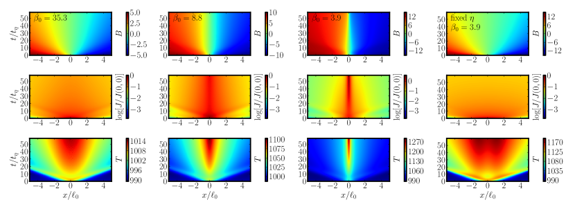
Figure 1.— Space-time evolution of $B$ in Gauss, self-normalized current density, and $T$ in K for three different values of initial $\beta_{0}$, with a background temperature of $T_{0}=990$ K. In the fixed $\eta$ case, the ionization level is set to that from the background non-thermal ionization.

4. Results

In Figure 1 we show the space-time evolution of the instability as a function of the ratio of thermal to magnetic pressure

$$\beta=8\pi\rho_{0}kT_{0}/(\mu m_{p}B_{0}^{2}),$$ (39)

with and without temperature dependent resistivity. In the third column we see the typical nature of the instability: a strong current sheet develops, shown by the narrowing of the magnetic field. When the temperature dependent ionization is turned off (column 4) the reconnection region diffuses outwards normally. We also see a difference between this system and the idealized one of Section 2.3: the current density in the center spreads resistively at early times so the background current is not constant in time. The difference between columns 3 and 4 shows the importance of treating the temperature dependence of the resistivity in this system.

4.1. Growth Rate

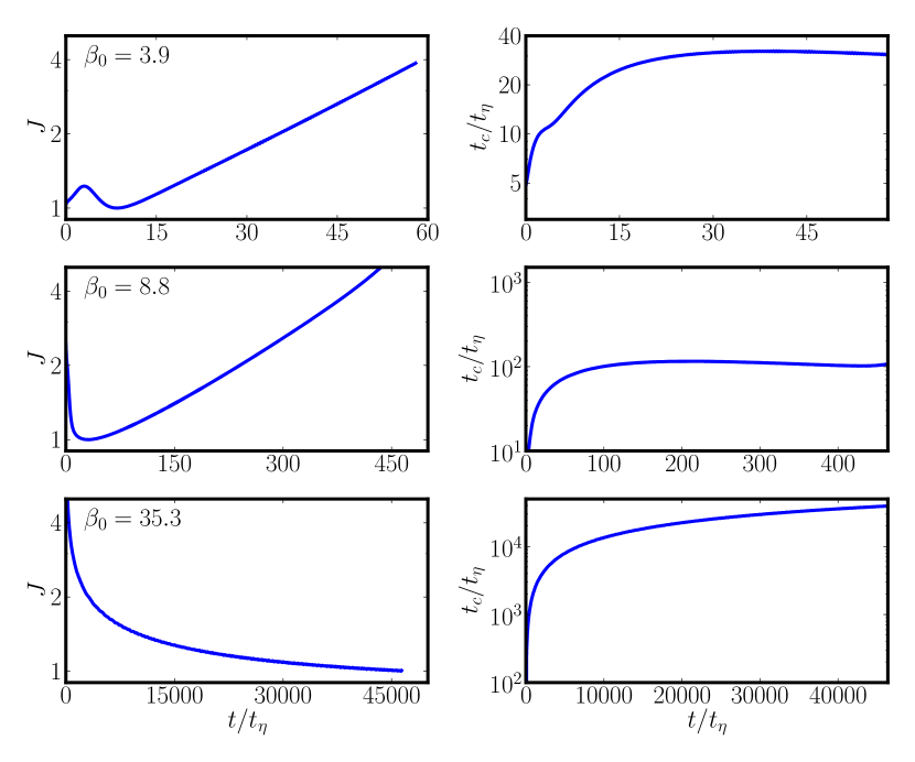
Figure 2.— Top panels: $\beta_{0}=4.9$; Middle panels: $\beta_{0}=18.6$; Bottom panels: $\beta_{0}=37.5$. Left panels: Time variation of J at the origin, normalized to its minimum value. Right panels: the dynamically defined timescale $t_{c}$, normalized to the resistive time $t_{\eta}$. All for three values of $\beta_{0}$ given in the panels and a background temperature of $T_{0}=990$ K.

We can use the linear growth rate given by Equation (23) to estimate the growth rate of the instability in the nonlinear regime reached in the simulations. In this regime, the value of the growth rate $\lambda(x,t)$ depends strongly on both position and time because of the variation of the parameters, especially $\eta$, but also the initial resistive spreading of the current density (see Figure 1). We extend to the nonlinear case by computing the value of $\lambda(0,t)$ at the center of the current sheet and examining it to see if it saturates to a constant value in the nonlinear regime that provides a reliable estimate of the actual growth rate. We define a timescale $t_{c}(t)=\lambda^{-1}(0,t)$ that we use to test this hypothesis.

In the following computation of $t_{c}$, we use $\ell\equiv\max(B)/J(x=0)$ as the approximate, time-varying, width of the current sheet, taking the place of $k^{-1}$ in the linear analysis, and

$$\beta_{c}=\frac{8\pi n_{n}k_{B}T}{\max(B^{2})},$$ (40)

$$t_{r,c}=\ell^{2}/\eta,$$ (41)

$$t_{h,c}=\frac{\beta_{c}}{\gamma-1}\frac{t_{r,c}}{2},$$ (42)

$$t_{\eta^{\prime},c}=\frac{T}{T_{i}}t_{h,c},$$ (43)

where all spatially varying quantities are determined at $x=0$. Solving Equation (23) for $\lambda$ using the above definitions, we find

$$(1/t_{c})= \frac{1}{2t_{r,c}}\left\{\vphantom{\left[\left(\frac{2T_{i}}{T}\right)^{2}\right]^{1/2}}-\left(1+\frac{2T_{i}}{T}\frac{\gamma-1}{\beta_{c}}\right)+\right.$$ (44)

$$\left.\left[1+\frac{12T_{i}}{T}\frac{\gamma-1}{\beta_{c}}+\left(\frac{2T_{i}}{T}\frac{\gamma-1}{\beta_{c}}\right)^{2}\right]^{1/2}\right\}^{-1}.$$

In Figure 2 we plot $J(0)$, and $t_{c}$, normalizing by the resistive time at the start of the simulation, $t_{\eta}\equiv t_{r,c}(t=0)$. We can see that $t_{c}(t)$ is reasonably well behaved and indeed has a defined plateau that occurs after the onset of current density growth. On the other hand, it initially grows significantly because of the resistivity drop caused by Ohmic heating. As $t_{c}$ possesses a defined maximum value in systems that show current density growth, we will use its maximum value for our estimate of the growth rate. Unfortunately, this is not strictly well defined in cases that do not show current density growth (e.g. Figure 2, bottom panel).

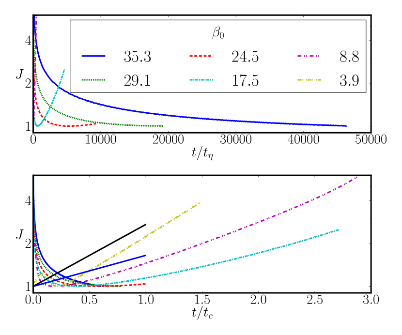
Figure 3.— Time series of J at the origin, normalized to its minimum value for two different time normalizations and six values of $\beta_{0}$. The background temperature of these models is $T_{0}=990$ K. The solid, straight curves show $\exp(t/t_{c})$ and $\exp(t/2t_{c})$.

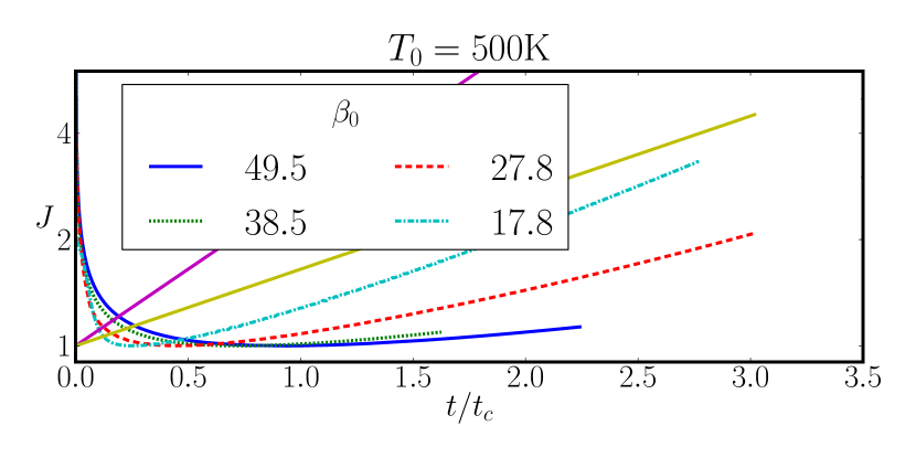
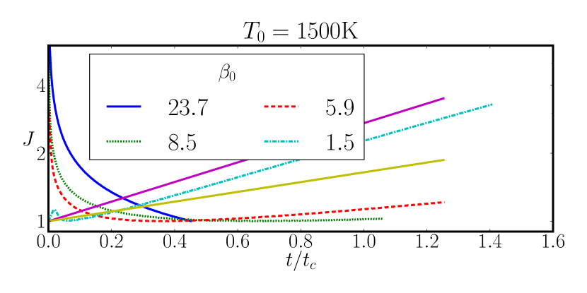
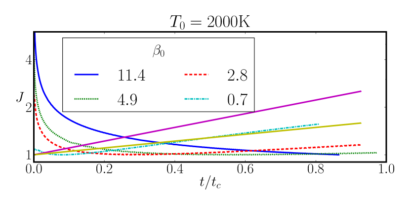
Figure 4.— Time series of J at the origin, normalized to its minimum value, for three background temperatures, $T_{0}=500,\,1500$, and 2000 K.

In Figures 3 and 4 we show the evolution of the central current density $J$ for four temperatures and varying $\beta_{0}$. Further, we include the functions $\exp(t/t_{c})$ and $\exp(t/2t_{c})$. If the analysis of Section 2.3 were exactly applicable with our definition of $t_{c}$, then the growing instabilities would have the slope of the former. It is clear that, although $t_{c}$ is a reasonable estimate of the timescale for instability growth, the curves of growing $J$ do not all have the same slope, and $t_{c}$ overestimates growth rates in some cases. Recall that $t_{c}$ is not well defined for the runs that fail to go unstable.

The fact that $t_{c}$ is a good estimate of the growth rate of the instability is perhaps surprising in light of the behavior of the resistivity (Figure 5, bottom panel). As the instability grows the resistivity at the origin drops by nearly two orders of magnitude, while the current sheet gets strongly concentrated: the system has become strongly nonlinear. A possible explanation for the continued relevance of the linear analysis, however, is that the symmetry of the model problem maintains the validity of the assumptions in Section 2.3. In particular, the current sheet concentrated by the instability has a flat current density at the origin that acts as the background current density for further growth. We discuss this further in Section 4.3 below.

4.2. Stability Criterion

From Section 2.3 we might expect that all our simulations should be unstable due to the lack of cooling. While Figures 3 and 4 show runs that have not gone unstable, it is unclear whether this is due to the additional physics that we have added to the problem changing the condition for instability, or merely inadequate run time (note that longer run times require larger boxes to exile the boundaries to infinity). The growth rate does appear to drop with increasing $\beta_{0}$ even when normalized to $t_{c}$. This slower growth may be due to the lower value of $t_{r,c}/t_{c}$ in the high $\beta_{0}$ case (see Equation 44). Unlike in the linear analysis, the resistive time also acts to spread the background current sheet and will decrease the instability’s growth rate, and may halt it altogether.

However, in Figure 3, top panel, the curve associated with $\beta_{0}=9.9$ is just distinguishable from the left axis, while the curve associated with $\beta=4.9$ is not. Clearly the increase in instability growth time with $\beta_{0}$ is pronounced, with the lowest obviously unstable $\beta_{0}=25.6$ presented having its instability kick in at $t\sim 5000t_{\eta}$. We expect that higher $\beta_{0}$s, if unstable, would require even longer. Even if the higher $\beta_{0}$ runs are eventually unstable, it is unlikely to be a matter of practical concern in a physical system. We attribute this to the longer interval in which the resistive spreading term in Equation (4) dominates over the instability term, resulting in an ever increasing $\ell$, and so an ever decreasing $\lambda$.

4.3. Saturation

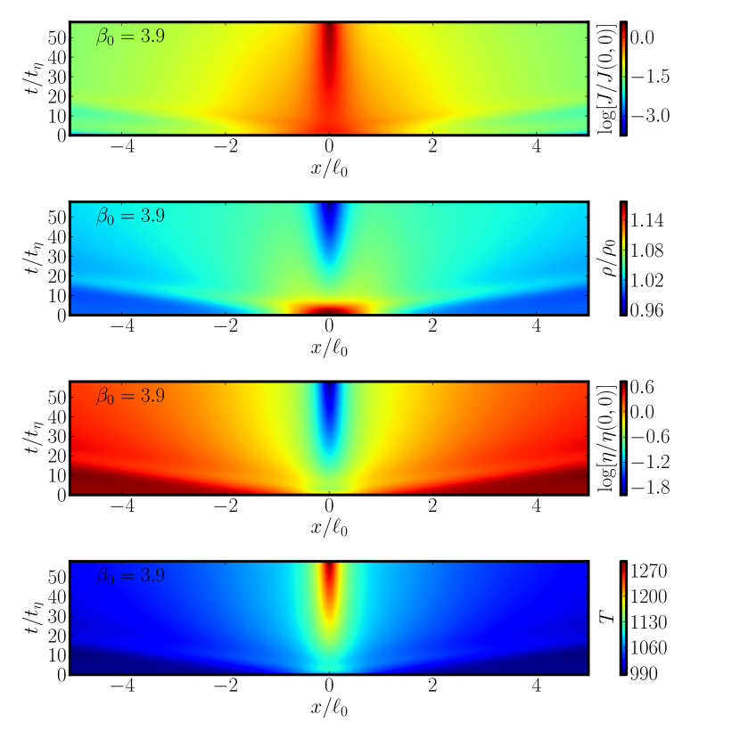
Figure 5.— Self normalized current density, mass density, and resistivity, and temperature in Kelvins, for $\beta_{0}=3.9$ and a background temperature of $990$ K. Note that the density drops in the central region implying mass outflow from the central region even while magnetic flux is transported inwards (as traced by the growing current).

Figure 6.— Magnetic field (Gauss), and current density plots for $\beta_{0}=2.2$ and a background temperature of $990$ K. Top panels: $dx/\ell_{0}=0.004$; Bottom panels: $dx/\ell_{0}=0.002$. On the right panels, the x-axes are in grid points rather than position (logarithmic spacing) but the plots cover the same physical extent. We can see the high resolution run continuing to narrow after the low resolution run has hit the grid scale and started ringing, as shown by the sooty dashes at the very top of the top-right panel.

In the absence of cooling and ever decreasing resistivity, it is not clear how the instability can saturate. So long as the current density $J$ remains differentiable at the origin, symmetry requires that $\partial_{x}J=0$, so the approximation assumed in Section 2.3 remains good. The saturated instability must maintain the constant background current assumed. Further, as we can see in Figure 5, while the system is compressible, it is not very compressible, with $\rho T$ approximately constant. This sustained satisfaction of the linear instability criterion may explain why the time-scale estimate $t_{c}$, which is determined from a linear stability analysis, performs as well as it does despite the non-perturbative evolution of the system shown in Figure 5.

In Figure 6 we show the evolution of the same system at two different resolutions, with the magnetic field plotted according to physical position on the left, and on the right, the current density plotted according to position on the logarithmically spaced grid. The upper panels show models with minimum grid resolution $dx=0.004\,\ell_{0}$ while the lower panels have $dx=0.002\,\ell_{0}$. The physical extent associated with the right panels is the same for the two resolutions and the same mapping of current density to color is used. In the left panels, we show the initial field, and the narrowing associated with the growing current sheet, which evolves similarly at both resolutions. In the right panels, we show the current density reaching the innermost grid point (the left side of the plot is the mirror image of the right) at low resolution, and associated ringing, while the high resolution run continues to narrow. It too will eventually narrow to below its grid resolution and be subject to the same numerical instability.

In the absence of cooling, or changing physics, such as an alteration to the resistivity equation, it appears that the instability will not saturate. If the background current density is constant in time and differentiable at the origin, symmetry requires that it have a constant component which is linearly unstable in the absence of cooling. Formally, the $\eta\mbox{\boldmath$\nabla$}{}^{2}\mbox{\boldmath$B$}{}$ term in the induction equation (3) prohibits non-differentiable current densities, so that the actual saturation mechanism must involve changing physics.

One clear possibility is that the action of cooling in combination with a change in the temperature dependence of $\eta$ should halt the instability, as cooling will become stronger at higher temperatures while the resistivity temperature gradient weakens. At high temperatures, it is expected that the temperature dependence of resistivity will change from that given by Equations (32) and (33). As the ionization fraction approaches full ionization, the temperature dependence of the resistivity will weaken. If the ionization fraction saturates, then the current sheet instability itself will saturate.

5. Discussion and Conclusions

We have shown that in slab-symmetric reconnection, a strong inverse temperature dependence of the resistivity can lead to an instability that concentrates the current in a narrow, high temperature, low resistivity sheet. This scenario is the polar opposite of the more common situation where the resistivity appears to increase inside current sheets through some anomalous resistivity (Krall & Liewer, 1971; Sato & Hayashi, 1979). Unlike many reconnection scenarios, the inward transport of the magnetic field in our case is resistive rather than advective in nature, sidestepping issues of fluid pile up that occur with advective field transport, as demonstrated by Figure 5, where the central density declines with time.

However, rather than speeding the dissipation of magnetic energy into heat, in one dimension the total dissipation rate actually falls, thanks to the formation of small volumes with very low resistivity, even though heating increases sharply within those regions. This raises interesting questions about the structure of magnetic turbulence in three-dimensional systems with similar temperature dependent resistivities.

The instability does not grow extremely fast as can be seen in Figure 2, which shows that the instability growth rate estimate $t_{c}$ is significantly slower than the background resistive broadening time of the current sheet $t_{\eta}$. Nevertheless, as seen clearly in the third column of Figure 1, the instability can grow on timescales of tens of resistive times. For this to occur, the strength of the magnetic field must allow rapid heating, and external large-scale dynamics must not tear the current sheet apart. Both of these conditions appear reasonable for disks subject to the MRI (Sano, 2007). Further, it is clear from Figure 1 that a fully self-consistent analysis is needed for any MRI active region in a protoplanetary disk whose magnetic field and temperature flirt with $\beta\sim 1-4$ and $T\sim 1000$ K. We have only considered growth of the instability in approximations to current sheets that the MRI generates in the absence of our instability. Such a self-consistent approach will be difficult considering the large range in dissipation parameters that must be resolved and the large spatial scale separation between the turbulence (larger than $\ell_{0}$) and the narrowed current sheets (much smaller than $\ell_{0}$, Fig 6).

We expect such self-consistent systems to show the concentration of current into localized regions with high current and temperature (either two-dimensional sheets or one-dimensional tubes), with the rest of space taken up by almost force-free magnetic fields. As the concentrated current regions have low resistivity, they could potentially have long lifetimes, perhaps much longer than that associated with the high wavenumber tail of a subsonic turbulent cascade. Where the magnetic field energy does not exceed equipartition with the fluid kinetic energy, the bending of the magnetic field will create new current structures that fence in the magnetic field configuration, with the potential for extremely large and localized Lorentz forces because of the highly concentrated current densities.

While we have shown that, in sufficiently restricted circumstances, this instability occurs for any inverse relationship between the resistivity and the temperature, we have also shown that it can take a prohibitive time to set in. In practice it appears that the growth rate estimate of Equation (23), while sometimes an overestimate, is accurate within factors of a few. Unfortunately, evaluating it requires that the instability be growing, and any initial transients can result in strong overestimates of the growth rate (see Figure 2, early times).

We explore the peak temperatures achieved by this instability further in Paper II, in particular by including radiative transfer and a fuller treatment of thermal ionization. However the significance for protoplanetary temperature structures in the inner MRI active disk is already clear from the work presented here.

Although we have considered this effect from the perspective of protoplanetary disks, it should occur in any system with an adequately strongly increasing conductivity dependence on temperature when compared to available cooling. Candidates include cool stellar surfaces with poorly ionized hydrogen, and even planetary atmospheres, as recently suggested by Menou (2012).

References

- Balbus & Hawley (1991) Balbus, S. A., & Hawley, J. F. 1991. ApJ, 376, 214–233.
- Balbus & Hawley (1998) Balbus, S. A., & Hawley, J. F. 1998, Rev. Mod. Phys., 1–53.
- Balbus & Terquem (2001) Balbus, S. A., & Terquem, C. 2001,ApJ, 552, 235–247.
- Beckwith & Sargent (1993) Beckwith, S. V. W., & Sargent, A. I. 1993. Protostars and Planets III, eds. E. Levy & J. I. Lunine (Tucson: U. of AZ), 521–541.
- Boss (1996) Boss, A. P. 1996, ApJ, 469, 906
- Brandenburg & Zweibel (1994) Brandenburg, A., & Zweibel, E. G. 1994, ApJ, 427, L91
- Brownlee et al. (2006) Brownlee, D. et al. (including Ebel, D.) 2006, Science 314, 1711–1717.
- Chandrasekhar (1961) Chandrasekhar, S. 1961. Hydrodynamic and Hydromagnetic Stability (Oxford: Clarendon), 384.
- Connolly et al. (1998) Connolly, H.C. Jr., Jones, B. D., & Hewins, R. H. 1998. Geochim. Cosmochim. Acta 62, 2725–2735.
- Cowley et al. (1997) Cowley, S. C., Longcope, D. W., & Sudan, R. N. 1997. Phys. Rep. 283, 227–251.
- Desch & Cuzzi (2000) Desch, S. J., & Cuzzi, J. N. 2000, Icarus, 143, 87
- Dullemond & Monnier (2010) Dullemond, C. P., & Monnier, J. D. 2010, ARA&A, 48, 205
- Ebel (2006) Ebel, D.S. 2006, Meteorites & the Early Solar System II, eds. D. Lauretta et al. (Tucson: U. of AZ), 253–277.
- Fleming and Stone (2003) Fleming, T., & Stone, J. M. 2003. ApJ, 585, 908–920.
- Flock et al. (2011) Flock, M., Dzyurkevich, N., Klahr, H., Turner, N. J., & Henning, T. 2011, ApJ, 735, 122
- Fromang et al. (2002) Fromang, S., Terquem, C., & Balbus, S. A. 2002. MNRAS, 329, 18–28.
- Gammie (1996) Gammie, C. F. 1996. ApJ, 457, 355–362.
- Glassgold et al. (1997) Glassgold, A. E., Najita, J., & Igea, J. 1997. ApJ, 480, 344–350 (Erratum, 485, 920).
- Harris (1962) Harris, E., 1962, Nuovo Cimento 23, 115.
- Hartmann (1998) Hartmann, L. 1998, Accretion Processes in Star Formation (Cambridge: Cambridge U. Press).
- Hindmarsh et al. (2005) Hindmarsh, A. C., Brown, P. N., Grant, K. E., Lee, S. L., Serban, R., Shumaker, D. E., Woodward, C. S. 2005. ACM Trans. Math. Softw., 31 3, 363–396.
- Hirose & Turner (2011) Hirose, S., & Turner, N. J. 2011.ApJ, 732, L30 (5 pp).
- Horanyi et al. (1995) Horanyi, M., Morfill, G., Goertz, C. K., & Levy, E. H. 1995, Icarus, 114, 174.
- Ilgner and Nelson (2006) Ilgner, M., & Nelson, R. P. 2006. A&A, 455, 731–740.
- King & Pringle (2010) King, A. R., & Pringle, J. E. 2010. MNRAS, 404, 1903–1909.
- Krall & Liewer (1971) Krall, N. A., & Liewer, P. C. 1971, Phys. Rev. A, 4, 2094
- Lazerson (2010) Lazerson, S. A. 2010, PhD Thesis, University of Alaska at Fairbanks
- Levy & Araki (1989) Levy, E. H., & Araki, S. 1989, Icarus, 81, 74
- Lodato & Rice (2004) Lodato, G., & Rice, W. K. M. 2004. MNRAS, 351, 630.
- Lofgren and Lanier (1990) Lofgren, G., Lanier, A. B. 1990. Geochim. Cosmochim. Acta 54, 3537.
- Malfait et al. (1998) Malfait, K., Waelkens, C., Waters, L. B. F. M., Vandenbussche, B., Huygen, E., & de Graauw, M. S. 1998. A&A, 332, L25.
- Malyshkin & Zweibel (2011) Malyshkin, L. M., & Zweibel, E. G. 2011, ApJ, 739, 72
- McNally (2012a) McNally, C. P. 2012, PhD thesis, Columbia University
- McNally et al. (2012b) McNally, C. P., Hubbard, A., & Mac Low, M.-M. 2012, ApJ, submitted.
- Muranushi (2010) Muranushi, T. 2010, MNRAS, 401, 2641
- Muranushi et al. (2012) Muranushi, T., Okuzumi, S., & Inutsuka, S.-i. 2012, ApJ, in press (arXiv:1210.2508)
- Menou (2012) Menou, K. 2012, ApJ (Letters), in press (arXiv:1206.3363)
- Nakamura et al. (2008) Nakamura T., Noguchi T., Tsuchiyama A., Ushikubo T., Kita N.T., Valley J.W., Zolensky M.E., Kakazu Y., Sakamoto K., Mashio E., Uesugi K., and Nakano T. 2008, Science, 321, 1664–1667.
- Oishi & Mac Low (2009) Oishi, J. S., & Mac Low, M.-M. 2009. ApJ, 704, 1239.
- Parker (1972) Parker, E. N. 1972. ApJ, 174, 499.
- Parker (1994) Parker, E. N. 1994. Spontaneous Current Sheets in Magnetic Fields: With Applications to Stellar X-rays. (Oxford: Oxford U. Press).
- Pilipp et al. (1998) Pilipp, W., Hartquist, T. W., Morfill, G. E., & Levy, E. H. 1998, A&A, 331, 121
- Price et al. (2012) Price, S., Link, B., Epstein, R. I., & Li, H. 2012, MNRAS, 420, 949
- Radomsky and Hewins (1990) Radomsky, P. M., & Hewins, R. H. 1990. Geochim. Cosmochim. Acta 54, 3475.
- Romanova (2011) Romanova, M. M. 2011. Bull. Amer. Astron. Soc. 43, #104.04.
- Romanova et al. (2011) Romanova, M. M., Ustyugova, G. V., Koldoba, A. V., & Lovelace, R. V. E. 2011. MNRAS, 416, 416–438.
- Sano et al. (2000) Sano, T., Miyama, S. M., Umebayashi, T., & Nakano, T. 2000. ApJ, 543, 486–501.
- Sano (2007) Sano, T. 2007, Ap&SS, 307, 191
- Sargent et al. (2009) Sargent, B. A., Forrest, W. J., Tayrien, C., et al. 2009, ApJS, 182, 477
- Sato & Hayashi (1979) Sato, T., & Hayashi, T. 1979, Physics of Fluids, 22, 1189
- Scott & Krot (2005) Scott E. R. D., & Krot, A. N. 2005, Chondrites and the Protoplanetary Disk, eds. A. N. Krot, E. R. D. Scott, B. Reipurth (San Francisco: Astronomical Society of the Pacific), 15–80.
- Shakura & Sunyaev (1973) Shakura, N. I., & Sunyaev, R. A. 1973, A&A, 24, 337
- Simon et al. (2008) Simon S.B., Joswiak D.J., Ishii H.A., Bradley J.P., Chi M., Grossman L., Aléon, Brownlee D.E., Fallon S., Hutcheon I.D., Matrajt G., McKeegan K.D. 2008, Met. & Plan. Sci., 43, 1861–1877.
- Turner & Drake (2009) Turner, N. J. & J. F. Drake. 2009. ApJ, 703: 2152–2159.
- Umebayashi & Nakano (2009) Umebayashi, T. & Nakano, T. 2009. ApJ, 690, 69–81.
- Van Boekel et al. (2004) Van Boekel, R., et al. 2004. Nature, 432, 479–482.
- Velikhov (1959) Velikhov, E. P. 1959. Sov. Phys. JETP, 36, 995–998.
- Waelkens et al. (1996) Waelkens, C., Waters, L.B.F.M., de Graauw, M.S., Huygen, E., Malfait, K., Plets, H., Vandenbussche, B., Beintema, D.A., Boxhoorn, D.R., Habing, H.J., Heras, A.M., Kester, D.J.M., Lahuis, F., Morris, P.W., Roelfsema, P.R., Salama, A., Siebenmorgen, R., Trams, N.R., van der Bliek, N.R., Valentijn, E.A., & Wesselius, P.R.: 1996, A&A, 315, L245–L248.
- Whipple (1966) Whipple, F. L. 1966. Science 153, 54.
- Yamada et al. (2010) Yamada, M., Kulsrud, R., & Ji, H. 2010. Rev. Mod. Phys., 82, 603–664.
- Zolensky et al. (2006) Zolensky M. E. et al. 2006. Science, 314, 1735–1739.
- Zweibel et al. (2011) Zweibel, E. G., Lawrence, E., Yoo, J., et al. 2011, Physics of Plasmas, 18, 111211