The Zeroth Law of Thermodynamics and Volume-Preserving Conservative System in Equilibrium with Stochastic Damping

Abstract

We propose a mathematical formulation of the zeroth law of thermodynamics and develop a stochastic dynamical theory, with a consistent irreversible thermodynamics, for systems possessing sustained conservative stationary current in phase space while in equilibrium with a heat bath. The theory generalizes underdamped mechanical equilibrium: $dx=gdt+\{-D\nabla\phi dt+\sqrt{2D}dB(t)\}$, with $\nabla\cdot g=0$ and $\{\cdots\}$ respectively representing phase-volume preserving dynamics and stochastic damping. The zeroth law implies stationary distribution $u^{ss}(x)=e^{-\phi(x)}$. We find an orthogonality $\nabla\phi\cdot g=0$ as a hallmark of the system. Stochastic thermodynamics based on time reversal $\big{(}t,\phi,g\big{)}\rightarrow\big{(}-t,\phi,-g\big{)}$ is formulated: entropy production $e_{p}^{\#}(t)=-dF(t)/dt$; generalized “heat” $h_{d}^{\#}(t)=-dU(t)/dt$, $U(t)=\int_{\mathbb{R}^{n}}\phi(x)u(x,t)dx$ being “internal energy”, and “free energy” $F(t)=U(t)+\int_{\mathbb{R}^{n}}u(x,t)\ln u(x,t)dx$ never increases. Entropy follows $\frac{dS}{dt}=e_{p}^{\#}-h_{d}^{\#}$. Our formulation is shown to be consistent with an earlier theory of P. Ao. Its contradistinctions to other theories, potential-flux decomposition, stochastic Hamiltonian system with even and odd variables, Klein-Kramers equation, Freidlin-Wentzell’s theory, and GENERIC, are discussed.

1 Introduction

Newtonian deterministic dynamics of particles and Gibbs’ statistical treatment of heterogeneous equilibrium matters are two of the most important mathematical theories of physical phenomena in one’s daily experiences. In recent years, there has been a significant progress in a mathematical theory of dynamics and thermodynamics of mesoscopic systems with a Markov-process description. This theory is slowly becoming a part of the dynamic branch of Gibbs’ program which had started more than a century before.

The stochastic thermodynamics encompasses two types of nonequilibrium phenomena: one is a transient, non-stationary stochastic processes approaching to an equilibrium, and another is a stationary, ergodic nonequilibrium steady state (NESS) with sustained energy input balanced by dissipation [1, 2, 3, 4, 5, 6]. Taking stochastic fluctuations into account, the theory characterizes three distinct temporal behaviors: non-stationary transient relaxation, stationary fluctuating equilibrium with zero entropy production, and stationary fluctuating NESS with positive entropy production. The theory has already found natural applications in biochemical signal processing inside living cells [7, 8, 9], free energy transduction in motors proteins [10, 5], and other molecular machines [1].

In mathematical terms, however, the definition of a “stochastic equilibrium” is far from universally agreed upon [11]. In Newtonian conservative dynamic theory, any system as a whole is automatically in an equilibrium, in a thermodynamic sense — there is simply no transient behavior, nor dissipation. A transient phenomenon in this perspective only occurs in a subsystem. With the presence of “frictions” phenomenologically defined, the equilibrium of a subsystem is the long-time behavior after damping with energy loss. However, a closer look indicates that there are two very different types of dynamic behavior in a mechanical equilibrium: an overdamped system with no oscillations and an underdamped system with continuous cyclic motion in $(p,q)$ phase space.

On the other hand, one of the major successes of stochastic dynamics is in the chemistry and biochemistry of single macromolecule in aqueous solution with overdamped dynamics, e.g., the Flory-Rouse-Zimm polymer theory [12, 13] and its NESS generalization [14, 15]. They are sometime collectively called soft matters in physics [16]. While overdamped stochastic dynamics is extensively studied with wide applications, underdamped systems with both conservative oscillations and stochastic damping [17, 18, 19, 20, 21] have been studied only within physics community. This includes, for examples, laser physics, electrical circuits, Josephson junctions, nanomechanical resonators, etc. [22, 23]. Many such systems exhibit stochastic resonance phenomena due to an interplay between stochastic dynamics and nonlinear oscillations [24, 25, 3].

All those above mentioned systems have a second-order dynamics in which two types of variables, $p_{i}(t)$ and $q_{i}(t)$ are identified a priori. In a more abstract mathematical theory where variables $\{x_{j}(t)|j=1,2,\cdots\}$ are not distinguished, detailed balance has been a widely used mathematical criterion for equilibrium, for example in chemistry [26, 27, 28]. However, detailed balance condition in stochastic processes in fact depends upon identifying even and odd dynamic variables, a notion first proposed by Casimir in analogous to positions and velocities in classical mechanics [29]. In the context of Markov dynamics, they first appeared as $\alpha$ and $\beta$ variables in the work of Machlup and Onsager [30], then studied by van Kampen [19], Graham and Haken [21], and more recently in [31, 32, 33, 34, 35, 36]. For a brief summary of this matter, readers are referred to [37].

Furthermore, a canonical form of stochastic Hamiltonian dynamics with weak (under-)damping is a diffusion process represented by the Klein-Kramers equation, the Kolmogorov forward equation for a second-order Newton’s equation of motion in a stochastic medium with frictions and random collisions. As a system of stochastic differential equations (SDE), the diffusion matrix is singular in the Klein-Kramers equation. Generalizing this approach encounters a mathematical difficulty due to the degeneracy of the diffusion: The existence of an equilibrium ensemble is often difficult to establish with some rigor.

This paper presents a mathematical theory that generalizes underdamped equilibrium stochastic dynamics, together with an irreversible thermodynamics, whose applicability goes beyond traditional Hamiltonian systems [38]. Insteady of starting with a second-order stochastic differential equation and using detailed balance as the equilibrium constraint, we approach an underdamped stochastic dynamics from a rather different starting point. In nonlinear dynamical systems theory, a conservative system with volume-preserving flow in phase space, $\dot{x}=g(x)$ where $\nabla\cdot g(x)=0$, is the natural generalization of Hamiltonian dynamics [38, 40, 41, 42]. When coupled to an stochastic damping with friction and collisions, it is natural to consider a stochastic differential equation (SDE)

$$dx(t)=g(x)dt+\Big{\{}-D\nabla\phi(x)dt+d\xi(t)\Big{\}}$$ (1)

in which the terms inside $\{\cdots\}$, in the spirit of P. Langevin [43], represent the mean “friction” and rapid “collision” of the stochastic damping: $\langle\xi(t)\xi(t^{\prime})\rangle=2D\delta(t-t^{\prime})$.

We focus on systems that approach to an equilibrium with stationary current. To introduce equilibrium condition into the stochastic setting, the present work departures from the traditional enforcing of fluctuation-dissipation relation to Eq. (1). Instead, we generalize the idea of the zeroth law of thermodynamics which states that two systems in equilibrum are essentially unaltered whether they are in contact with or detached from each other: We assume that the stationary density of the system (1), $u^{ss}(x)$, has to be the same with and without the damping part:

$$u^{ss}(x)=e^{-\phi(x)}.$$ (2)

Eq. (1) shows that its stationary state is invariant under an additive constant $\phi(x)\rightarrow\phi(x)+C$. The constant $C$ will be chosen such that the $u^{ss}(x)$ in Eq. (2) is normalized.

Eq. (2) generalized the notion of the zeroth law. It shares the same spirit as detailed balance in statistical chemistry [26, 27, 28], fluctuation-dissipation relation in statistical physics [44, 45, 46], and J. Wyman’s thermodynamic linkage in macromolecular biochemistry [47]: If a bath is in equilibrium with a system, then the equilibrium bath is invariant irrespective of whether it is in contact with the system or not. A nonequilibirum steady state arises only when the condition in (2) is violated due to a dis-equilibrium between the bath and the conservative dynamical system [18, 31]. Such a supposition underlies many of recent studies on second-order (e.g., underdamped) stochastic dynamics [31, 32, 33, 34, 35, 36]; its violation constitutes an active driving force, e.g., a feedback control or a Maxwell’s demon, from a nonequilibrium environment [48].

Introduced as above, an equilibrium stochastic system possesses an important orthogonal relation between $\nabla\phi$ and $g$. To show this, we write the Kolmogorov forward equation for the SDE in (1):

$$\frac{\partial u(q,t)}{\partial t}=\nabla\cdot\Big{[}D\nabla u-\Big{(}g(x)-D\nabla\phi(x)\Big{)}u\Big{]}.$$ (3)

Then Eq. 2 implies $-\nabla\cdot\big{[}g(x)u^{ss}\big{]}=u^{ss}(x)\big{(}g(x)\cdot\nabla\phi\big{)}=0$. Therefore, for dynamics with $u^{ss}(x)>0$, the equilibrium condition implies the orthogonality. The stationary current is $g(x)u^{ss}(x)$.

Sec. 2 of the paper provides the mathematical basis for a “conservative stochastic thermodynamics” in the presence of stationary probability current [49]. Based on a new form of time reversal motivated by Hamiltonian dynamics, $\big{(}t,\phi,g\big{)}\rightarrow\big{(}-t,\phi,-g\big{)}$ for Eq. 1 [29], a measure-theoretical entropy production $e_{p}^{\#}$ is introduced in Eq. 8. We show that it equals to the decreasing rate of a generalized free energy functional $-dF/dt$, where [49]

$$F\big{[}u(x,t)\big{]}=\int_{\mathbb{R}^{n}}u(x,t)\ln\Big{(}u(x,t)e^{\phi(x)}\Big{)}dx.$$ (4)

$-dF/dt$, which is non-negative, has been called free energy dissipation in [50, 51] and non-adiabatic entropy production in [52, 53, 54]. In the stationary state, $e_{p}^{\#}\equiv 0$, and the probability current is analogous to the inertia in mechanics and magnetic induction in electrical circuits [22].

In 2004, P. Ao proposed a novel form of a non-detailed-balanced stochastic process together with a decomposition scheme that yields stationary probability density and stationary current, as well as a steady state thermodynamics [55, 49]:

$$\Big{[}S(x)+A(x)\Big{]}\frac{dx}{dt}=-\nabla\phi(x)+\zeta(x,t),\ \ \ x\in\mathbb{R}^{n}$$ (5a)

in which

$$\langle\zeta(x,t)\zeta^{T}(x,t^{\prime})\rangle=2S(x)\delta(t-t^{\prime}).$$ (5b)

One of the attractive features of Eq. (5ba) is its representation in terms of a symmetric matrix $S(x)$ and an antisymmetric matrix $A(x)$ along the stochastic path, potentially facilitating computations for such stochastic systems without detailed balance. However the author has never made the relationship clear between (5b) and the general stochastic differential equation

$$dx(t)=b(x)dt+\Gamma(x)dw(t).$$ (6)

Ao’s stochastic theory has intrigued and mystified many researchers; he and his coworkers have further carried out explicit computations for linear stochatsic differential equations following the general theory [56]. One of the key features in the linear system is an orthogonality between the gradient of stationary density and the stationary probability current. In Sec. 3, we shall show that the system in Eq. 5b is consistent with the stochastic dynamics with volume-preserving flow introduced in Eqs. 1, 2, and 3.

The theory we present is a synthesis of several known results. To clarify, we shall reiterate its novelty: It ($i$) develops a underdamped stochastic dynamics in the general term of dynamical systems without the need of a Hamiltonian, nor the identification of even and odd variables. The classical Klein-Kramers equation for stochastic Newtonian dynamics is simply a special case (see Sec. 4.1). ($ii$) mathematically formulated the zeroth law of thermodynamics as an equilibrium condition; ($iii$) derived an orthogonal relation between gradient $\nabla\phi$ and current $g$. Note this orthogonality is not the same as that obained in the Freidlin-Wentzell theory [57, 58], where the term corresponding to $g$ was not a divergence-free current in general (see Sec. 5.1). ($iv$) shows a consistency with the stochastic dynamical equation proposed by Ao in [55]; ($v$) introduced a trajectory-based entropy production formula using the time reversal $(t,\phi,g)\rightarrow(-t,\phi,-g)$ and derived irreversible thermodynamic equations (12) and (15) for the thermodynamics.

2 Stochastic thermodynamics

In a Hamiltonian system $\dot{q}=\partial H/\partial p$ and $\dot{p}=-\partial H/\partial q$, transformation $(q,p)\rightarrow(q,-p)$ is equivalent to transforming $H\rightarrow-H$ [40, 41, 42]. In the theory of diffusion process, the Kolmogorov forward equation for SDE (6) with stationary density $u^{ss}(x)$ is

$$\frac{\partial u(x,t)}{\partial t}=\nabla\cdot\left(A(x)u^{ss}(x)\nabla\left(\frac{u(x,t)}{u^{ss}(x)}\right)-\Big{\{}b(x)-A(x)\nabla u^{ss}(x)\Big{\}}u(x,t)\right),$$ (7)

in which $A(x)=\frac{1}{2}\Gamma(x)\Gamma^{T}(x)$. The time-reversed process to (6) satisfies the Kolmogorov equation with a sign-change for the divergence-free term in $\{\cdots\}$ [6]. These observations suggest that a meaningful time-reversed process for SDE in (1) is $(x,g)\rightarrow(x,-g)$, as illustrated in Fig. 1. The time reversal tranformation then is $(t,x,g)\rightarrow(-t,x,-g)$: The time-reversed process for time-reversed stochastic path. Also see Sec. 4.3 for more justifications.

In terms of such a time reversal, let us consider a stochatsic path $\omega_{[t,\tau]}=\big{\{}x(s)\big{|}t\leq s\leq\tau\big{\}}$ and its time-reversed path $r\omega_{[t,\tau]}=\big{\{}x(t+\tau-s)\big{|}t\leq s\leq\tau\big{\}}$ under the probability measures $\mathbb{P}^{+g}$ and $\mathbb{P}^{-g}$, rspectively, defined by SDEs $dX=\big{(}g-D\nabla\phi\big{)}dt+d\xi(t)$ and its time-reversal $dX^{-}=\big{(}-g-D\nabla\phi\big{)}dt+d\xi(t)$. Denoting $\mathbb{P}^{-}\big{(}\omega_{[t,\tau]}\big{)}$ $\equiv$ $\mathbb{P}^{-g}\big{(}r\omega_{[t,\tau]}\big{)}$, a sample-path based entropy production can be introduced [6, 54, 11, 59, 60, 61, 62]:

$$e_{p}^{\#}(t) = \lim_{\tau\rightarrow t}E^{\mathbb{P}^{+g}}\left[\frac{1}{|\tau-t|}\ln\frac{d\mathbb{P}^{+g}}{d\mathbb{P}^{-}}\big{(}\omega_{[t,\tau]}\big{)}\right]$$ (8)

$$= -\int_{\mathbb{R}^{n}}J(x,t)\cdot\nabla\ln\left(\frac{u(x,t)}{u^{eq}(x)}\right)dx,$$ (9)

$$= \int_{\mathbb{R}^{n}}u(x,t)\nabla\ln\Big{(}u(x,t)e^{\phi(x)}\Big{)}\cdot D\nabla\ln\Big{(}u(x,t)e^{\phi(x)}\Big{)}dx\ \geq\ 0,$$ (10)

where $J(x,t)=\big{(}g-D\nabla\phi\big{)}u(x,t)-D\nabla u(x,t)$, and $E^{\mathbb{P}^{+g}}\big{[}\cdots\big{]}$ denotes ensemble everage with respect to $\mathbb{P}^{+g}$. We note that the $g$ term has disappeared in the final expression: Entropy production is purely determined by the damping mechanism. Note that we have changed the notation $u^{ss}(x)$ to $u^{eq}(x)$ to emphasize that the steady state is an equilibrium with conservative current.

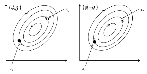
Figure 1: In stationarity with $\tau\geq t$, the joint probability distribution $\Pr\big{\{}X(t)=x_{1},X(\tau)=x_{2}\big{\}}$ for the diffusion process on the left, according (1) with $\big{(}\phi,g\big{)}$, i.e., $dX(t)=\big{(}g-D\nabla\phi\big{)}dt+d\xi(t)$ and $\nabla\phi\cdot g=0$, is the same as the joint probability distribution $\Pr\big{\{}X^{-}(t)=x_{2};X^{-}(\tau)=x_{1}\big{\}}$ for the diffusion process on the right, $X^{-}(t)$ with $\big{(}\phi,-g\big{)}$, under a time reversals: $\Pr\big{\{}X^{-}(-t)=x_{2};X^{-}(-\tau)=x_{1}\big{\}}$ $=$ $\Pr\big{\{}X^{-}(\tau-t)=x_{2};X^{-}(0)=x_{1}\big{\}}$ $=$ $\Pr\big{\{}X(0)=x_{1},X(\tau-t)=x_{2}\big{\}}$ $=$ $\Pr\big{\{}X(t)=x_{1};X(\tau)=x_{2}\big{\}}$. The closed cycles in both plots, the contours of $\phi$, are the same; the actual speed along a contour is determined by $\|g\|$.

It is important to point out that the $e_{p}^{\#}$ introdiced in Eq. 8 is different from the standard entropy production for a stochastic diffusion [11, 61, 62, 6]. In the literature, $e_{p}^{\#}$ has been called free energy dissipation or non-adiabatic entropy production [50, 52, 53, 54].

One can also define a generalized nonequilibrium free energy [6],

$$F(t)=\int_{\mathbb{R}^{n}}u(x,t)\ln\left(\frac{u(x,t)}{u^{eq}(x)}\right)\ dx.$$ (11)

Then in terms of the $e_{p}^{\#}$, it has been shown in [49] that:

$$\frac{dF(t)}{dt}=\int_{\mathbb{R}^{n}}J(x,t)\cdot\nabla\ln\left(\frac{u(x,t)}{u^{eq}(x)}\right)\ dx\ =\ -e_{p}^{\#}(t)\leq 0.$$ (12)

Eq. 12 should be interpreted as follows: For Gibbs’ canonical ensemble with non-uniform $u^{eq}(x)=e^{-\phi(x)}$, the thermodynamic potential is free energy $F$ whose decreasing rate is the entropy production $e_{p}^{\#}$.

The generalized nonequilibrium free energy $F(t)$ in (11) can be decomposed into $U(t)-S(t)$ with

$$U(t)=-\int_{\mathbb{R}^{n}}u(x,t)\ln u^{eq}(x)\ dx,\ \ S(t)=-\int_{\mathbb{R}^{n}}u(x,t)\ln u(x,t)\ dx.$$ (13)

They are interpreted as internal (conservative) energy and entropy, respectively. Furthermore,

$$\frac{dU}{dt}=-\frac{d}{dt}\left(\int_{\mathbb{R}^{n}}u(x,t)\ln u^{eq}(x)dx\right)=\int_{\mathbb{R}^{n}}\nabla\phi\cdot D\nabla\ln\Big{(}u(x,t)e^{\phi}\Big{)}\ dx.$$ (14)

We note again that the $g$ term has completely disappeared in Eqs. (13) and (14). The right-hand-side of (14) can be interpreted as “heat flux”, analogous to the heat in classical thermodynamics, $h_{d}^{\#}(t)$. Then,

$$\frac{dS}{dt}-e_{p}^{\#}(t)=-h_{d}^{\#}(t)=\frac{dU}{dt},$$ (15)

which is precisely the entropy balance equation in Dutch school of nonequilibrium thermodynamics [63]: $\frac{dS}{dt}=\frac{d_{i}S}{dt}+\frac{d_{e}S}{dt}$. See also [18] and [5] for discussions on the meanings of these terms as the system’s entropy change, total entropy prodction, and heat dissipation.

In mathematics, the functional $F\big{[}u(t)\big{]}$, as the Gibbs-Shannon entropy with respect to a non-uniform probability measure with density $u^{eq}$, is known to contain two a priori estimates, based on respectively the non-negativity of $F$ and $e_{p}^{\#}$ [64].

3 Conservative dynamics with stationary current and stochastic damping

The previous section has established a self-consistent underdamped stochastic thermodynamics with conservative stationary current. We now show that the stochastic dynamics defined in Eqs. (1), (2), and (3) with orthogonal $\nabla\phi$ and $g$, is consistent with Ao’s model (5b).

Without being mathematically rigorous, one can formally establish the relation between Eq. 5b and the conventional SDE (6): Introducing a transformation via an auxiliary matrix inversion $\big{(}S(x)+A(x)\big{)}^{-1}$ $=$ $G(x)$ one obtaines [55]

$$\frac{dx}{dt}=-G(x)\nabla\phi(x)+\xi(x,t),$$ (16)

with

$$\big{\langle}\xi(x,t)\xi^{T}(x,t^{\prime})\big{\rangle} = \Big{\langle}G(x)\zeta(x,t)\zeta^{T}(x,t^{\prime})G(x)^{T}\Big{\rangle}$$ (17)

$$= 2G(x)\ S(x)\ G^{T}(x)\ \delta(t-t^{\prime}).$$

Then the associated Kolmogorov partial differential equation in divergence form, following [65, 66], is,

$$\frac{\partial u(x,t)}{dt}=\nabla\cdot\Big{[}G(x)S(x)G^{T}(x)\nabla u+G(x)\nabla\phi(x)u\Big{]}.$$ (18)

One of the key results in [55] is that the stationary density for the stochastic process being $e^{-\phi(x)}$. Then the stationary current $J(x)$ satisfies [67, 51]

$$J(x)e^{\phi(x)}=G(x)S(x)G^{T}(x)\nabla\phi(x)-G(x)\nabla\phi(x).$$ (19)

From Eq. 19 one has

$$\big{(}\nabla\phi(x)\big{)}^{T}\cdot J(x)e^{\phi(x)} = \big{(}\nabla\phi(x)\big{)}^{T}\cdot\Big{[}GSG^{T}\nabla\phi(x)-G\nabla\phi(x)\Big{]}$$ (20)

$$= \Big{(}G^{T}\nabla\phi(x)\Big{)}^{T}\cdot\Big{[}-S+G^{-T}\Big{]}\Big{(}G^{T}\nabla\phi(x)\Big{)}$$

$$= \Big{(}G^{T}\nabla\phi(x)\Big{)}^{T}\cdot\Big{[}-S+S+A^{T}\Big{]}\Big{(}G^{T}\nabla\phi(x)\Big{)}$$

$$= 0.$$

Since $e^{\phi(x)}\neq 0$, Eq. 20 means $\big{(}\nabla\phi(x)\big{)}^{T}\cdot J(x)=0$ is a necessary condition for Ao’s stochastic model. It is a special case of the process introduced in Sec. 1.

4 Relations to other theories

An oscillatory motion in an overdamped mechanical system (e.g., a macromolecule in an aqueous solution) is due to external drive with dissipation; while an oscillatory motion in an underdamped system is a part of conservative dynamics. How to develop a mathematical thermodynamic theory for stochastic systems with stationary current, therefore, is a fundamental issue of mesoscopic dynamics [6]. Because of its centrality, there have been many theories that are relevant to the present work. We shall discuss several of them that we have studied.

4.1 Klein-Kramers equation and stochastic Hamiltonian dynamics

Following the seminal work of Langevin, Klein and Kramers, it is a custom to writes a stochastic Newtonian dynamics for a subsystem of 1-degree of freedom, with damping, as:

$$\left\{\begin{array}[]{l}dx=ydt,\\[5.0pt] mdy=-\left[\frac{dU(x)}{dx}+\eta(x)y\right]dt+\sqrt{k_{B}T\eta(x)}dB(t),\end{array}\right.$$ (21)

in which the coefficient of $dB(t)$ is fixed by Einstein’s relation, which guarantees Maxwell-Boltzmann stationary distribution $e^{-H(x,y)/k_{B}T}$ with $H(x,y)=\frac{1}{2}my^{2}+U(x)$. In the notations of our Eq. (1):

$$\vec{g}=\left(\begin{array}[]{c}y\\[5.0pt] -\frac{1}{m}U^{\prime}(x)\end{array}\right)=\frac{1}{m}\left(\begin{array}[]{cc}0&1\\[5.0pt] -1&0\end{array}\right)\nabla H,$$ (22)

$$\nabla\cdot\vec{g}=\frac{\partial}{\partial x}y-\frac{\partial}{\partial y}\left(\frac{U^{\prime}(x)}{m}\right)=0,$$ (23)

$$\phi=\frac{1}{k_{B}T}\left(\frac{my^{2}}{2}+U(x)\right),\ \ \nabla\phi=\frac{1}{k_{B}T}\Big{(}U^{\prime}(x),my\Big{)},$$ (24)

therefore, $\vec{g}\cdot\nabla\phi=0$.

In fact, one has a more general stochastic Hamiltonian system [39, 31]:

$$\frac{d}{dt}\left(\begin{array}[]{c}x\\[5.0pt] y\end{array}\right)=\left(\begin{array}[]{cc}\frac{\partial H}{\partial y}+\eta_{x}(x,y)\\[8.0pt] -\frac{\partial H}{\partial x}+\eta_{y}(x,y)\end{array}\right)+\Gamma(x,y)\left(\begin{array}[]{c}\frac{dw_{x}}{dt}\\[8.0pt] \frac{dw_{y}}{dt}\end{array}\right),$$ (25)

in which both $x$ and $y$ are $n$-dimensional vectors, and $\Gamma$ is a $2n\times 2n$ matrix. Then, following our formalism, the $2n$ vector

$$\vec{g}=\left(\begin{array}[]{c}\frac{\partial H}{\partial y}\\[6.0pt] -\frac{\partial H}{\partial x}\end{array}\right),$$ (26)

$\phi=-\ln u^{eq}$, and

$$\left[\frac{1}{2}\Big{(}\big{(}\nabla_{x},\nabla_{y}\big{)}\Gamma(x,y)\Gamma^{T}(x,y)\Big{)}^{T}-\left(\begin{array}[]{c}\eta_{x}(x,y)\\ \eta_{y}(x,y)\end{array}\right)\right]u^{eq}(x,y)=0.$$ (27)

Using (27), the Fokker-Planck equation for (25),

$$\frac{\partial u}{\partial t}=\big{(}\nabla_{x},\nabla_{y}\big{)}\left[\frac{1}{2}\Big{(}\big{(}\nabla_{x},\nabla_{y}\big{)}\Gamma(x,y)\Gamma^{T}(x,y)\Big{)}^{T}-\left(\begin{array}[]{c}\frac{\partial H}{\partial y}+\eta_{x}\\[8.0pt] -\frac{\partial H}{\partial x}+\eta_{y}\end{array}\right)\right]u,$$ (28)

can be written as

$$\frac{\partial u}{\partial t}=\big{(}\nabla_{x},\nabla_{y}\big{)}\left\{\frac{1}{2}\Gamma(x,y)\Gamma^{T}(x,y)\left[\left(\begin{array}[]{c}\nabla_{x}\\[6.0pt] \nabla_{y}\end{array}\right)-\left(\begin{array}[]{c}\nabla_{x}\ln u^{eq}\\[6.0pt] \nabla_{y}\ln u^{eq}\end{array}\right)\right]-\left(\begin{array}[]{c}\frac{\partial H}{\partial y}\\[8.0pt] -\frac{\partial H}{\partial x}\end{array}\right)\right\}u.$$ (29)

It is easy to verify that the orthogonal relation $\vec{g}\cdot\nabla\phi=0$ guarantees $e^{-H(x,y)}$ being the equilibrium solution to (29). This yields a fluctuation-dissipation relation like equation for stochastic damping:

$$\left(\begin{array}[]{c}\eta_{x}\\ \eta_{y}\end{array}\right)=\frac{1}{2}e^{H(x,y)}\Big{(}\big{(}\nabla_{x},\nabla_{y}\big{)}\Gamma(x,y)\Gamma^{T}(x,y)\Big{)}^{T}e^{-H(x,y)}.$$ (30)

Newtonian dynamics is a special case with singular $\Gamma$ [31]

$$\Gamma(x,y)\Gamma^{T}(x,y)=\left(\begin{array}[]{cc}0&0\\ 0&1\end{array}\right),\ \left(\begin{array}[]{c}\eta_{x}\\ \eta_{y}\end{array}\right)=\left(\begin{array}[]{c}0\\ -\nabla_{y}H(x,y)\end{array}\right).$$ (31)

Itō vs. divergence form. There are several mathematical choices for the intergration of an SDE with multiplicative noise, e.g., Itō, Stratonovich, or Ao’s divergence form [66]. We note that we started with Itō’s convention in Eq. (28). However withthe the zeroth law, the resulting Eq. (29) in fact is in the divergence form. The final partial differential equation in fact is independent of the choice of stochastic intergration. To see this more clearly, consider the Fokker-Planck equation for $dx=\big{(}g(x)+\eta(x)\big{)}dt+\sqrt{2D(x)}dB(t)$, in Itō’s form:

$$\frac{\partial u(x,t)}{\partial t}=\nabla\cdot\Big{[}\Big{(}\nabla\big{(}D(x)u(x,t)\big{)}-\eta(x)u(x,t)\Big{)}-g(x)u(x,t)\Big{]},$$ (32)

with $\eta(x)$ and $\phi(x)$ being related via

$$\nabla\Big{(}D(x)e^{-\phi(x)}\Big{)}-\eta(x)e^{-\phi(x)}=0.$$ (33)

Solving $\eta(x)$ from Eq. (33) and substituting it into (32), we have

$$\frac{\partial u(x,t)}{\partial t}=\nabla\cdot\Big{[}D(x)\Big{(}\nabla u(x,t)+u(x,t)\nabla\phi(x)\Big{)}-g(x)u(x,t)\Big{]}.$$ (34)

4.2 Wang’s Hodge-like decomposition

The orthogonality in Eq. 20 leads to several interesting properties for the stochastic dynamics. First, noting the SDE in (6) and the relation in (19), we have the drift

$$b(x)=-G(x)\nabla\phi(x)\ =\ -D\nabla\phi(x)+J(x)e^{\phi(x)},$$ (35)

and $\langle\xi(t)\xi(t^{\prime})\rangle=2D\delta\big{(}t-t^{\prime}\big{)}$. Denoting $g(x)=J(x)e^{\phi(x)}$, then

$$b(x)=-D\nabla\phi+g,\ \nabla\cdot g=0,\ \nabla\phi\cdot g=0.$$ (36)

The right-hand-side of (35) are Wang’s potential and flux landscapes [67, 51] for a general SDE. The orthogonality between the gradient and current terms is an additional feature of Ao’s stochastic processes. The first two equations in (36) are a Helmholtz-Hodge-like decomposition with diffusion matrix $D$ [68]. As far as we know, there is no orthogonality in a Hodge decomposition in general.

Xing’s Hamiltonian representation. For a Hamiltonian system, the orthogonality is a consequence of a damped Hamiltonian dynamics [18, 39] in equilibrium with detailed-balanced stochastic fluctuations. Then the stationary process defined by (28) has a distribution $u^{eq}=e^{-H}$ as well as a conservative rotation in phase space:

$$J(x,y)=-\left(\begin{array}[]{c}\frac{\partial H}{\partial y}\\[8.0pt] -\frac{\partial H}{\partial x}\end{array}\right)u^{eq}(x,y).$$ (37)

Indeed, $\nabla u^{eq}\cdot J=0$. Eqs. (27) and (28) are based on Itō’s integration. It is easy to see that if another convention for stochastic integration is chosen, both equations will have different expressions; but Eqs. (29) and (37) are invariant.

For any SDE (6) with stationary density $e^{-\phi}$ and flux $J$, if $\nabla\phi\cdot J=0$, then the SDE can be re-written as

$$dx(t)=\Big{\{}-D\nabla\phi(x)+d\xi(t)\Big{\}}+g(x)$$ (38)

in which the first two terms in the $\{\cdots\}$ can be “interpreted” as the heat bath with detailed balance. They are analogous to the mean “friction” and rapid “collision” in classical mechanics, defining the notions of dissipation and fluctuation in a general stochastic dynamics. The dynamics described by the $g(x)$, on the other hand, is a deterministic conservative system [40] with a volume preserving flow in phase space [38]:

$$\frac{d}{dt}\int_{\mathfrak{D}(t)}dx=\oint_{\partial\mathfrak{D}}g(x)\cdot d\vec{S}=\int_{\mathfrak{D}}\nabla\cdot g(x)\ dx=0.$$ (39)

Therefore, it is not surprising that Xing is able to represent Ao’s process mathematically as a very large, conservative Hamiltonian system in which stochastic damping corresponds to a harmonic bath [69]. One should not confuse this result, however, with the Hamiltonian dynamics that defines conditional most probable path in a diffusion process [70, 71]. The relation between these two Hamiltonian systems, if any, remains to be elucidated.

Grmela-Öttinger’s GENERIC. One can also re-write the general stochastic Hamiltonian system Eq. (25) as

$$\left(\begin{array}[]{c}dx\\[6.0pt] dy\end{array}\right)=\left[\left(\begin{array}[]{c}\frac{\partial H}{\partial y}\\[8.0pt] -\frac{\partial H}{\partial x}\end{array}\right)-\left(\begin{array}[]{cc}D_{xx}&D_{xy}\\[7.0pt] D_{yx}&D_{yy}\end{array}\right)\left(\begin{array}[]{c}\frac{\partial\phi}{\partial x}\\[8.0pt] \frac{\partial\phi}{\partial y}\end{array}\right)\right]dt+\left(\begin{array}[]{c}d\xi_{x}(t)\\[6.0pt] d\xi_{y}(t)\end{array}\right).$$ (40)

The deterministic part here has the GENERIC form proposed by Grmela and Öttinger [72]. The orthogonality has also figured prominently in the GENERIC structure which has a rich geometric interpretation.

4.3 Detailed balance in systems with even and odd variables

There have been extensive discussions on detailed balance in stochastic differential equation with even and odd variables. See earlier work [30, 18, 19, 20, 21], a nice summary in the textbook [37], and more recent papers [31, 32, 33, 73, 34, 35, 36]. Detailed balance for system with position $x$ and velocity $v$ is defined through a symmetry between the transtion $\big{(}\mbox{\boldmath$x$},\mbox{\boldmath$v$},t\big{)}\rightarrow\big{(}\mbox{\boldmath$x$}^{\prime},\mbox{\boldmath$v$}^{\prime},t+\tau\big{)}$ and transition $\big{(}\mbox{\boldmath$x$}^{\prime},-\mbox{\boldmath$v$}^{\prime},t\big{)}\rightarrow\big{(}\mbox{\boldmath$x$},-\mbox{\boldmath$v$}^{\prime},t+\tau\big{)}$. The detailed balance condition in an even-and-odd system is shown to be sufficient for the probability current ${\bf J}=-{\bf J}^{-}$ where the ${\bf J}^{-}$ is the stationary current under time reversal ([37], Eq. 5.3.53). Also, for constant diffusion matrix, the cross terms between even and odd variables are necessarily zero. Furthermore, the stationary solution is “solved” in [37] (Eq. 5.3.85). Finally, recognizing the orthogonal condition presented in the present work, their Eq. 5.3.82 can be simplied into $\sum_{i}\frac{\partial}{\partial x_{i}}I_{i}(\mbox{\boldmath$x$})=0$; where $I$ is our $g$.

4.4 Temperature and NESS systems in spatial contact

There have been continous efforts to introduce the concept of temperature into systems in NESS [74, 75, 76]. Most of these work focused on stochastic interacting particle systems, in which a temperature difference is natually defined as a spatial gradient. Two approaches have been employed: ($a$) Legendre transform in conjunction with an energy conservation, and ($b$) empirically establishing an intensive quantity via numerical computations. All these approaches are essentially “thermodynamic” in nature, while the zeroth law in the present work is formulated as a statement about stationary distributions. This is a much stronger consition. It is also applicable to chemical potential equilibration as well as temperature equilibration.

We note, however, that our orthogonality $\nabla\phi\cdot g=0$ is effectively a conservation law; therefore it will be interesting to explore the possibility of introducing an conjugate intensive quantity via Legendre transform. Also, the fact that any linear stochastic dynamical system automatically satisfies $\nabla\phi\cdot g=0$ [56] seems to sugget that a pseudo-temperature could be defined for system with linear irreversibility.

4.5 Three different types of time reversal

We now consider the general SDE in Eq. 6. In [6], we have introduced the notion of a canonical conservative dynamics with respect to a differentiable invariant density $u^{ss}(x)$: $\dot{x}=j(x)$ with $\nabla\cdot\big{(}u^{ss}(x)j(x)\big{)}=0$. The general SDE, when its stationary density is known, can always be re-written as [6, 37]

$$dx(t)=\Big{(}b(x)+D(x)\nabla\phi(x)\Big{)}dt+\Big{\{}-D(x)\nabla\phi(x)\ dt+d\xi(t)\Big{\}},$$ (41)

in which $e^{-\phi(x)}=u^{ss}(x)$ is the stationary density. Then $j(x)=b(x)+D(x)\nabla\ln\phi(x)$ is a canonical conservative dynamics with respect to $u^{ss}(x)$. [6] also shows that under time reveral $\big{(}t,\phi,j\big{)}\rightarrow\big{(}-t,\phi,-j\big{)}$, the system in (41) has again entropy production $e_{p}^{\#}(t)=-dF/dt$.

One can further decompose the term $j(x)$ into parallel and perpendicular to $\nabla\phi(x)$: $j(x)=j_{\parallel}(x)+j_{\perp}(x)$, with

$$j_{\parallel}(x)=\left(\frac{j(x)\cdot\nabla\phi(x)}{\|\nabla\phi(x)\|^{2}}\right)\nabla\phi(x),\ \ j_{\perp}(x)=j(x)-j_{\parallel}(x),$$ (42)

where $\nabla\phi(x)\cdot j_{\perp}(x)=0$. Then

$$b(x)=-D(x)\nabla\phi(x)+j_{\perp}(x)+j_{\parallel}(x).$$ (43)

The last term can also be written as

$$j_{\parallel}(x)=\left(\frac{\nabla\cdot j(x)}{\|\nabla\phi(x)\|^{2}}\right)\nabla\phi(x).$$ (44)

It represents the non-conservative nature of $j(x)$ [38]. According to time reversal $\big{(}t,\phi,j\big{)}\rightarrow\big{(}-t,\phi,j\big{)}$, all $j(x)$ contributes to stationary entropy production [11, 3]; and according to time reversal $\big{(}t,\phi,j\big{)}\rightarrow\big{(}-t,\phi,-j\big{)}$, there will be no stationary entropy production [6]. The present work and Eq. 43 suggests yet another time reversal: $\big{(}t,\phi,j_{\perp}\big{)}\rightarrow\big{(}-t,\phi,-j_{\perp}\big{)}$, under which stationary dissipation arises from $j_{\parallel}$. These three different time reversals reflect assumptions based on over-damped, non-damped or under-damped nature of a stationary dynamics of a subsystem. For systems with overdamped time reversibility, they have a potential condition $D^{-1}(x)b(x)=\nabla\phi$ and the stationary density is $e^{-\phi(x)}$ with zero stationary current. For systems with underdamped time reversibility, they have an orthogonal decompositon $b(x)=D(x)\nabla\phi+g$ with $\nabla\times g=0$ and $g\cdot D(x)\nabla\phi=0$. Then the stationary density and current are $e^{-\phi(x)}$ and $g(x)e^{-\phi(x)}$, respectively.

5 Discussion

5.1 Orthogonality for infinitesimal noise

We now consider a general SDE with an infinitesimal stochastic term:

$$dx(t)=b(x)dt+\sqrt{\epsilon}d\xi(t),\ \ \big{\langle}\xi(t)\xi(t^{\prime})\big{\rangle}=2D\delta(t-t^{\prime}),$$ (45)

with Fokker-Planck equation

$$\frac{\partial u(x,t)}{\partial t}=-\nabla\cdot J(x,t),\ \ J(x,t)=b(x)u(x,t)-\epsilon D\nabla u(x,t).$$ (46)

The large deviation principle suggests that [57, 58, 77, 71]

$$u^{ss}(x)=\exp\left(-\frac{\psi_{\epsilon}(x)}{\epsilon}\right),$$ (47)

and thus, $J^{ss}(x)=u^{ss}(x)\big{(}b(x)+D\nabla\psi_{\epsilon}(x)\big{)}$. Then $\nabla\cdot J^{ss}(x)=0$ implies

$$\epsilon\nabla\cdot\Big{(}b(x)+D\nabla\psi_{\epsilon}(x)\Big{)}=\Big{(}b(x)+D\nabla\psi_{\epsilon}(x)\Big{)}\cdot\nabla\psi_{\epsilon}(x).$$ (48)

Reversibility under time reversal $\big{(}t,\phi,g\big{)}\rightarrow\big{(}-t,\phi,g\big{)}$ is eqivalent to $g=b+D\nabla\psi_{\epsilon}=0$ [11, 3], which is also known as potential condition [21, 37] . In the present work with time reversal $\big{(}t,\phi,g\big{)}\rightarrow\big{(}-t,\phi,-g\big{)}$, $g\neq 0$ but $\nabla\cdot g=g\cdot\nabla\psi_{\epsilon}=0$. One could consider these conditions as more general “solvability conditions” for the steady state of a stochastic dynamics.

Eq. 48 is exact. We now consider the limit of small $\epsilon$, and $\psi_{\epsilon}(x)=\phi_{0}(x)+\epsilon\phi_{1}(x)+\cdots$, where

$$\nabla\phi_{0}(x)\cdot\big{(}D\nabla\phi_{0}(x)+b(x)\big{)}=0,$$ (49)

$$\nabla\phi_{1}(x)\cdot\Big{(}2D\nabla\phi_{0}(x)+b(x)\Big{)}=\nabla\cdot\Big{(}D\nabla\phi_{0}(x)+b(x)\Big{)},$$ (50)

$$\nabla\phi_{2}(x)\cdot\Big{(}2D\nabla\phi_{0}(x)+b(x)\Big{)}=\nabla\cdot\Big{(}D\nabla\phi_{1}(x)\Big{)}-\big{(}\nabla\phi_{1}(x)\big{)}D\big{(}\nabla\phi_{1}(x)\big{)}.$$ (51)

We thus have a decomposition:

$$b(x)=-D\nabla\phi_{0}(x)+\Big{(}b(x)+D\nabla\phi_{0}(x)\Big{)},$$ (52)

in which the two terms are orthogonal by the definition of $\phi_{0}(x)$, as given in (49). This is a well-known result in the theory of large deviation [57, 71]. The second, however, is not divergence free. Actually, Eq. 48 indicates that, in the limit of $\epsilon\rightarrow 0$, $\nabla\cdot\big{(}b(x)+D\nabla\phi_{0}(x)\big{)}$ is $\frac{0}{0}$. In fact, from (50)

$$\nabla\cdot\Big{(}b(x)+D\nabla\phi_{0}(x)\Big{)}=-\nabla\phi_{1}(x)\cdot\Big{(}2D\nabla\phi_{0}(x)+b(x)\Big{)}$$ (53)

is on the order $O(1)$. Only when $\phi_{1}(x)\equiv$ a constant, the equation in (52) becomes an orthogonal Helmholtz-Hodge decomposition in the asymptotic limit of $\epsilon\rightarrow 0$. Ao’s stochastic process has all $\phi_{i}(x)=0$ with $i\geq 1$.

5.2 Boltzmann’s thermodnamic probability and Kolmogorov backward equation

Motivated by Eq. 14, let us introduce $\Omega(x,t)=u(x,t)e^{\phi(x)}$. Then

$$\frac{\partial\Omega(x,t)}{\partial t}=\nabla\cdot D\nabla\Omega(x,t)-\Big{(}g(x)+D\nabla\phi(x)\Big{)}\cdot\nabla\Omega(x,t).$$ (54)

The Kolmogorov backward equation corresponding to (34) is

$$\frac{\partial v(x,t)}{\partial t}=\nabla\cdot D\nabla v(x,t)-\Big{(}D\nabla\phi(x)-g(x)\Big{)}\cdot\nabla v(x,t).$$ (55)

They differ only by a $g\rightarrow-g$. The function $\Omega(x,t)$ can be interpreted as Boltzmann’s “thermodynamic probability”, whose logarithm is a thermodynamic potential (Boltzmann entropy). Finally, the probability current consists of a “mechanical” force $g$ and an “entropic” force $-D\nabla\ln\Omega$:

$$j(q,t)=g(x)-D\nabla\ln\Omega(x,t).$$ (56)

We also note that for both Eqs. 54 and 55, if $v(x,t)>0$, there is an Boltzmann’s H-theorem like relation:

$$\frac{d}{dt}\int_{\mathbb{R}^{n}}\Big{(}\Omega(x,t)\ln\Omega(x,t)\Big{)}e^{-\phi(x)}dq=-\int_{\mathbb{R}^{n}}\big{(}\nabla\Omega\big{)}\cdot\big{(}D\nabla\Omega\big{)}\left(\frac{e^{-\phi}}{\Omega}\right)dx\leq 0.$$ (57)

5.3 Conservative and dissipative dynamics

The notions of conserative and dissipative systems are fundamental concepts in mechanics and thermodynamics. They are the core of the world view based on Newtonian mechanics [82, 83, 84]. Entropy production is the key mathematical quantity characterizing dissipation. Since 1980s, it has become increasingly clear that the mathematical foundation of entropy production lies within the notion of time reversal [11, 59, 60, 61, 62].

For the dynamics associated with system in (1), classical Newtonian notion of time reversal is $\big{(}t,\phi,g\big{)}\rightarrow\big{(}-t,\phi,-g\big{)}$ which gives rise to an entropy production $e_{p}^{\#}$ solely by the non-adiabatic part $-dF/dt$. On the other hand, if one chooses time reversal $\big{(}t,\phi,g\big{)}\rightarrow\big{(}-t,\phi,g\big{)}$, then total entropy production $e_{p}$ is the sum of both adiabatic and non-adiabatic entropy productions [50, 54]. The adiabatic part is also known as house-keeping heat [85]: It represents the amount of active energy input to sustain a nonequilibrium steady state [6].

To put the above discussion into sharper contrast, consider the following biophysical experiment on a single motor protein in the presence of given ATP and ADP concentrations in solution [10]. At 100 cycles per second, a motor protein runs for a day with a total $\sim 10^{7}$ ATP hydrolysis. However, at a millimolar concentration in a millilitre volume, there are $10^{17}$ total number of ATP molecules. Hence, with a single motor protein running for a day in such a mesoscopic system, the concentration of ATP changes only 1 part of 10 billion. It is essentially undetectable.

Now consider an experiment on a type II superconducting ring with a current in the presence of a magnet. This system has been considered in condensed matter physics as an equilibrium system. However, according to Newton’s third law, the supercurrent has to exert a force on the magnet and causing it to slowly demagnetize even though it is essentially undetectable [86].

Newton’s first law states that a linear constant motion persists in the absence of a force. A rotatinal motion, hence, requires a force, even when it does no work. According to Newton’s third law and our understanding of the constituents of matter, there is always a consequence, à la Lord Kelvin, at the origin of the force field that causes the rotational motion, i.e., a stationary current. The environment of a system with sustained rotational motion, therefore, can not be absolutely time reversible.

Conservative or dissipative thermodynamic description of an open subsystem are mathematical models which depend upon an experimentalist’s knowledge and perspective. They are rather theoretical issues; the dynamics is closer to the reality.

I thank Ping Ao, Dick Bedeaux, Zhen-Qing Chen, Mark Dykman, Massimiliano Esposito, Hao Ge, Da-Quan Jiang, Signe Kjelstrup, David Lacoste, H.-C. Öttinger, Masaki Sasai, Udo Seifert, Jin Wang, and Jianhua Xing for many helpful discussions. I also thank Professor Madeleine Dong (University of Washington) for continuous dialogues on the nature of interpretations, narratives, and discourse in historical research.

References

- [1] Seifert, U. (2012) Stochastic thermodynamics, fluctuation theorems and molecular machines. Rep. Prog. Phys. 75, 126001.
- [2] Esposito, M. (2012) Stochastic thermodynamics under coarse graining. Phys. Rev. E 85, 041125.
- [3] Zhang, X.-J., Qian, H. and Qian, M. (2012) Stochastic theory of nonequilibrium steady states and its applications (Part I). Phys. Rep. 510, 1–86.
- [4] Santillán, M. and Qian, H. (2011) Irreversible thermodynamics in multiscale stochastic dynamical systems. Phys. Rev. E 83, 041130.
- [5] Ge, H. and Qian, H. (2013) Heat dissipation and nonequilibrium thermodynamics of quasi-steady states and open driven steady state. Phys. Rev. E 87, 062125.
- [6] Qian, H. (2013) A decomposition of irreversible diffusion processes without detailed balance. J. Math. Phys. 54, 053302.
- [7] Ge, H., Qian, M. and Qian, H. (2012) Stochastic theory of nonequilibrium steady states and its applications (Part II): Applications in chemical biophysics. Phys. Rep. 510, 87–118.
- [8] Lan, G., Sartori, P., Neumann, S., Sourjik, V. and Tu, Y. (2012) The energy-speed-accuracy trade-off in sensory adaptation. Nature Phys. 8, 422–428.
- [9] Mehta, P. and Schwab, D.J. (2013) Energetic costs of cellular computation. Proc. Natl. Acad. Sci. USA 109, 17978–17982.
- [10] Chowdhury, D. (2013) Stochastic mechano-chemical kinetics of molecular motors: A multidisciplinary enterprise from a physicist’s perspective. Phys. Rep. 529, 1–197.
- [11] Jiang, D.-Q., Qian, M. and Qian, M.-P. (2004) Mathmatical Theory of Nonequilibrium Steady States, LNM 1833, Springer, New York.
- [12] Doi, M. and Edwards, S.F. (1986) The Theory of Polymer Dynamics, Clarendon, Oxford.
- [13] Schellman, J.A. (1997) Thermodynamics, molecules and the Gibbs conference. Biophys. Chem. 64, 7–13.
- [14] Qian, H. (2002) Mesoscopic nonequilibrium thermodynamics of single macromolecules and dynamic entropy-energy compensation. Phys. Rev. E 65, 016102.
- [15] Qian, H. (2002) Equations for stochastic macromolecular mechanics of single proteins: Equilibrium fluctuations, transient kinetics and nonequilibrium steady-state. J. Phys. Chem. B 106, 2065–2073.
- [16] Kleman, M. and Lavrentovich, O. D. (2003) Soft Matter Physics: An Introduction, Springer, New York.
- [17] Wax, N. (1954) Selected Papers on Noise and Stochastic Processes. Dover, New York.
- [18] Bergmann, P.G. and Lebowitz, J.L. (1955) New appproach to nonequilibrium processes. Phys. Rev. 99, 578–587.
- [19] van Kampen, N.G. (1957) Derivation of the phenomenological equations from the master equation. II. Even and odd variables. Physica 23, 816–824.
- [20] Uhlhorn, U. (1960) Onsager’s reciprocal relations for nonlinear systems. Arkiv. Fysik. 17, 361–368.
- [21] Graham, R. and Haken, H. (1971) Fluctuations and stability of stationary nonequilibrium systems in detailed balance. Zeit. Phys. 245, 141–153.
- [22] Luchinsky, D.G. and McClintock, P.V.E. (1997) Irreversibilityof classical fluctuations studied in analogue electrical circuits. Nature, 389, 463–466.
- [23] Chan, H.B., Dykman, M.I. and Stambaugh, C. (2008) Paths of fluctuation induced switching. Phys. Rev. Lett. 100, 130602.
- [24] Gammaitoni, L., Hänggi, P., Jung, P. and Marchesoni, F. (1998) Stochastic resonance. Rev. Mod. Phys. 70, 223–287.
- [25] Dykman, M.I., Luchinsky, D.G., Mannella, R., McClintock, P.V.E., Stein N.D. and Stocks N.G. (1993) Nonconventional stochastic resonance. J. Stat. Phys. 70, 479–499.
- [26] Lewis, G.N. (1925) A new principle of equilibrium. Proc. Natl. Acad. Sci. USA 11, 179–183.
- [27] Fowler, R.H. and Milne, E.A. (1925) A note on the principle of detailed balancing. Proc. Natl. Acad. Sci. USA 11, 400–402.
- [28] Tolman, R.C. (1925) The principle of microscopic reversibility. Proc. Natl. Acad. Sci. USA 11, 436–439.
- [29] Casimir, H.B.G. (1945) On Onsager’s principle of microscopic reversibility. Rev. Mod. Phys. 17, 343–350.
- [30] Machlup, S. and Onsager, L. (1953) Fluctuations and irreversible processes. II. Systems with kinetic energy. Phys. Rev. 91, 1512–1515.
- [31] Kim, K.H. and Qian, H. (2004) Entropy production of Brownian macromolecules with inertia. Phys. Rev. Lett. 93, 120602.
- [32] Kim, K.H. and Qian, H. (2007) Fluctuation theorems of a molecular refrigerator. Phys. Rev. E 75, 022102.
- [33] Kwon, C., Noh, J.D. and Park, H. (2011) Nonequilibrium fluctuations for linear diffusion dynamics. Phys. Rev. E 83, 061145.
- [34] Spinney, R.E. and Ford, I.J. (2012) Entropy production in full phase space for continuous stochastic dynamics. Phys. Rev. E 85, 051113.
- [35] Munakata, T. and Rosinberg, M.L. (2012) Entropy production and fluctuation theorems under feedback control: The molecular refrigerator model revisited. J. Stat. Mech. Th. Exp. P05010.
- [36] Ge, H. (2012) Time reversibility and nonequilibrium thermodynamics of second-order stochastic systems with inertia. arXiv.org/abs/1209.3081
- [37] Gardiner, G.W. (2004) Handbook of Stochastic Methods for Physic, Chemistry and the Natural Sciences, 3rd ed., Springer, New York.
- [38] Andrey, L. (1985) The rate of entropy change in non-Hamiltonian systems. Phys. Lett. A 111, 45–46.
- [39] Qian, M. (1979) The invariant measure and ergodic property of a Markov semigroup (in Chinese). Beijing Daxue Xuebao, 2, 46–59.
- [40] Strogatz, S.H. (2001) Nonlinear Dynamics And Chaos: With Applications To Physics, Biology, Chemistry, And Engineering. Westview Press, Boulder, CO.
- [41] Berger, A. (2001) Chaos and Chance: An Introduction to Stochastic Aspects of Dynamics. Walter de Gruyter, Berlin.
- [42] Gaspard, P. (2005) Chaos, Scattering and Statistical Mechanics. Cambridge Univ. Press, U.K.
- [43] Coffey, W.T., Kalmykov, Y.P. and Waldron, J.T. (1996) The Langevin Equation. World Scientiffc, Singapore.
- [44] Callen, H.B. and Welton, T.A. (1951) Irreversibility and generalized noise. Phys. Rev. 83, 34–40.
- [45] Wyman, J. (1965) The binding potential, a neglected linkage concept. J. Mol. Biol. 11, 631–644.
- [46] Kubo, R. (1966) The fluctuation-dissipation theorem. Rep. Prog. Phys. 29, 255–284.
- [47] Di Cera, E., Gill, S.J. nad Wyman, J. (1988) Canonical formulation of linkage thermodynamics. Proc. Natl. Acad. Sci. USA 85, 5077–5081.
- [48] Qian, H. (2012) Cooperativity in cellular biochemical processes: Noise-enhanced sensitivity, fluctuating enzyme, bistability with nonlinear feedback, and other mechanisms for sigmoidal responses. Ann. Rev. Biophys. 41, 179–204.
- [49] Ao, P. (2008) Emerging of stochastic dynamical equalities and steady state thermodynamics from Darwinian dynamics. Commun. Theor. Phys. 49, 1073–1090.
- [50] Ge, H. and Qian, H. (2010) The physical origins of entropy production, free energy dissipation and their mathematical representations. Phys. Rev. E, 81, 051133.
- [51] Feng, H. and Wang, J. (2011) Potential and flux decomposition for dynamical systems and non-equilibrium thermodynamics: Curvature, gauge field, and generalized fluctuation-dissipation theorem. J. Chem. Phys. 135, 234511.
- [52] Hatano, T. and Sasa, S.-I. (2001) Steady-state thermodynamics of Langevin systems. Phys. Rev. Lett. 86, 3463–3466.
- [53] Chernyak, V.Y., Chertkov, M. and Jarzynski, C. (2006) Path-integral analysis of fluctuation theorems for general Langevin processes. J. Stat. Mech. Th. Exp. P08001.
- [54] van den Broeck, C. and Esposito, M. (2010) The three faces of the Second Law: II. Fokker-Planck formulation. Phys. Rev. E 82, 011144.
- [55] Ao, P. (2004) Potential in stochastic differential equations: Novel construction. J. Phys. A: Math. Gen. 37, L25-L30.
- [56] Kwon, C., Ao, P. and Thouless, D.J. (2005) Structure of stochastic dynamics near fixed points. Proc. Natl. Acad. Sci. USA 102, 13029–13033.
- [57] Ventsel’, A.D. and Freidlin, M.I. (1970) On small random perturbations of dynamical systems. Russ. Math. Surv. 25(1), 1–55.
- [58] Graham, R. and Tél, T. (1984) Existence of a potential for dissipative dynamical systems. Phys. Rev. Lett. 52, 9–12.
- [59] Qian, M.-P. and Qian, M. (1985) The entropy production and irreversibility of Markov processes. Chin. Sci. Bull. 30, 445–447.
- [60] Crooks, G. (1999) Entropy production fluctuation theorem and the nonequilibrium work relation for free energy differences. Phys. Rev. E. 60, 2721–2726.
- [61] Seifert, U. (2005) Entropy production along a stochastic trajectory and an integral fluctuation theorem. Phys. Rev. Lett. 95, 040602.
- [62] Ge, H. and Jiang, D.-Q. (2007) The transient fluctuation theorem of sample entropy production for general stochastic processes. J. Phys. A: Math. Theor. 40, F713-F723.
- [63] de Groot, S.R. and Mazur, P. (1962) Non-equilibrium Thermodynamics, North-Holland, Amsterdam.
- [64] Villani, C. (2008) H-theorem and beyond: Boltzmann’s entropy in today’s mathematics. In Boltzmann’s Legacy, Gallavotti, G., Reiter, W.L. and Yngvason, J. eds., European Math. Soc. Pub., Zürich, pp. 129–143.
- [65] Yin, L. and Ao, P. (2006) Existence and construction of dynamical potential in nonequilibrium processes without detailed balance. J. Phys. A: Math. Gen. 39, 8593–8601.
- [66] Yuan, R. and Ao, P. (2012) Beyond Itō vs. Stratonovich. J. Stat. Mech. Th. Exp. P07010.
- [67] Wang, J., Xu, L. and Wang, E. (2008) Potential landscape and flux framework of nonequilibrium networks: Robustness, dissipation, and coherence of biochemical oscillations. Proc. Natl. Acad. Sci. U.S.A. 105,12271–12276.
- [68] Qian, M. and Wang, Z.-D. (1999) The entropy production of diffusion processes on manifolds and its circulation decompositio. Comm. Math. Phys. 206, 429–445.
- [69] Xing, J. (2010) Mapping between dissipative and Hamiltonian systems. J. Phys. A: Math. Th. 43, 375003.
- [70] Wang, J., Zhang, K. and Wang, E. (2010) Kinetic paths, time scale, and underlying landscapes: A path integral framework to study global natures of nonequilibrium systems and networks. J. Chem. Phys. 133, 125103.
- [71] Ge, H. and Qian, H. (2012) Analytical mechanics in stochastic dynamics: Most probable path, large-deviation rate function and Hamilton-Jacobi equation. Int. J. Mod. Phys. B 26, 1230012.
- [72] Grmela, M. and Öttinger, H.C. (1997) Dynamics and thermodynamics of complex fluids. I. Development of a general formalism. Phys. Rev. E. 56, 6620-6632.
- [73] Kwon, C. and Ao, P. (2011) Nonequilibrium steady state of a stochastic system driven by a nonlinear drift force. Phys. Rev. E 84, 061106.
- [74] Bertin, E., Dauchot, O. and Droz, M. (2006) Definition and relevance of nonequilibrium intensive thermodynamic parameters. Phys. Rev. Lett. 96, 120601.
- [75] Shokef, Y., Shulkind, G. and Levine, D. (2007) Isolated nonequilibrium systems in contact. Phys. Rev. E 76, 030101R.
- [76] Pradhan, P., Amann, C. P. and Seifert, U. (2010) Nonequilibrium steady states in contact: Approximate thermodynamic structure and zeroth law for driven lattice gases. Phys. Rev. Lett. 105, 150601.
- [77] Dykman, M.I., Mori, E., Ross, J. and Hunt, P.M. (1994) Large fluctuations and optimal paths in chemical kinetics. J. Chem. Phys. 100, 5735–5750.
- [78] Ruelle, D. (1997) Entropy production in nonequilibrium statistical mechanics. Comm. Math. Phys. 189, 365–371.
- [79] Gallavotti, G. (2008) Entropy, nonequilibrium, chaos and infinitesimals. In Boltzmann’s Legacy, Gallavotti, G., Reiter, W.L. and Yngvason, J. eds., European Math. Soc. Pub., Zürich, pp. 39–60.
- [80] Jiang, D.-Q., Qian, M. and Qian, M.-P. (2000) Entropy production and information gain in axiom-A systems. Comm. Math. Phys. 214, 389–409.
- [81] Cowieson, W. and Young, L.-S. (2005) SRB measures as zero-noise limits. Ergod. Theory Dyn. Syst. 25, 1115–1138.
- [82] Prigogine, I and Stengers, I. (1984) Order Out of Chaos, New Sci. Lib. Shambhala Pub., Boulder, CO.
- [83] Pagels, H.R. (1985) Is the irreversibility we see a fundamental property of nature? Phys. Today 38(Jan), 97–99.
- [84] Bricmont, J. (1995) Science of chaos or chaos of science? Ann. N.Y. Acad. Sci. 775, 131–175.
- [85] Oono, Y. and Paniconi, M. (1998) Steady state thermodynamics. Prog. Theor. Phys. Supp. 130, 29–44.
- [86] Ao, P. and Zhu, X.-M. (1999) Microscopic theory of vortex dynamics in homogeneous superconductors. Phys. Rev. B 60, 6850–6877.