Radio AGN in galaxy clusters: heating hot atmospheres and driving supermassive black hole growth over cosmic time

Abstract

We estimate the average radio-AGN (mechanical) power deposited into the hot atmospheres of galaxy clusters over more than three quarters of the age of the Universe. Our sample was drawn from eight major X-ray cluster surveys, and includes 685 clusters in the redshift range $0.1<z<0.6$ that overlap the area covered by the NVSS. The radio-AGN mechanical power was estimated from the radio luminosity of central NVSS sources, using the relation of Cavagnolo et al. (2010) that is based on mechanical powers determined from the enthalpies of X-ray cavities. We find only a weak correlation between radio luminosity and cluster X-ray luminosity, although the most powerful radio sources resides in luminous clusters. The average AGN mechanical power of $3\times 10^{44}$$\rm\,erg\,s^{-1}$  exceeds the X-ray luminosity of $44\%$ of the clusters, indicating that the accumulation of radio-AGN energy is significant in these clusters. Integrating the AGN mechanical power to redshift $z=2.0$, using simple models for its evolution and disregarding the hierarchical growth of clusters, we find that the AGN energy accumulated per particle in low luminosity X-ray clusters exceeds $1$ keV per particle. This result represents a conservative lower limit to the accumulated thermal energy. The estimate is comparable to the level of energy needed to “preheat” clusters, indicating that continual outbursts from radio-AGN are a significant source of gas energy in hot atmospheres. Assuming an average mass conversion efficiency of $\eta=0.1$, our result implies that the supermassive black holes that released this energy did so by accreting an average of $\sim 10^{9}M_{\odot}$ over time, which is comparable to the level of growth expected during the quasar era.

1. Introduction

Models for the formation and evolution of cosmic structure generally invoke some heating mechanism to prevent catastrophic gas cooling and excessive star formation in massive galaxies (e.g., Sijacki & Springel, 2006). In galaxy clusters, the same mechanism may generate the excess entropy responsible for deviations from the self-similar scaling relations expected otherwise (e.g., Markevitch, 1998). For example, the $L_{\rm X}$ – $T$ relation for galaxy groups is steeper ($L_{\rm X}\propto T^{2.6}$; Markevitch, 1998) than for clusters ($L_{\rm X}\propto T^{2}$; Kaiser, 1986; Arnaud & Evrard, 1999). Excess entropy is also revealed by flatter core entropy profiles in galaxy groups than in massive clusters (e.g., Voit & Donahue, 2005). Furthermore, in cooling core clusters, the heating rate needs to be related to the high rate of radiative cooling that was previously thought to cause cooling flows (Fabian, 1994). The heating cannot be too effective, since cooling cores are found in a large fraction of local X-ray clusters (e.g., Mittal et al., 2009; Hudson et al., 2010; Santos et al., 2010), but it must be sufficient to explain the scarcity of cooling gas that would be expected to accompany strong cooling flows (e.g., Peterson et al., 2003).

One of the most promising sources of this non-gravitational energy is active galaxy nuclei (AGN; e.g., McNamara et al., 2000). The questions remain of when, how and and how much AGN energy is distributed into their environments (e.g., Short et al., 2012; Young et al., 2011). The preheating model (Evrard & Henry, 1991; Kaiser, 1991) proposes that energy injected into the intergalactic medium at high redshifts explains the observed departures from self-similar scaling relations. Wu et al. (2000) found that the minimum excess energy required to break self-similarity is $\simeq 1$ keV/particle. At high redshifts, many AGN are in the radiatively efficient “quasar” mode (Croton et al., 2006), when high AGN accretion rates are promoted by the high galaxy merger rate. Although most of the energy output of these AGN is radiated away, quasars are so powerful that only a small fraction of this energy is required to produce the excess entropy in hot atmospheres. By contrast, there are far fewer quasars at lower redshifts, but X-ray observations have revealed that AGN in “radio mode” deposit significant amounts of energy into their hot atmospheres. The total energy output of AGN in radio mode is generally less than in quasar mode. Nevertheless, a large proportion of this emerges as mechanical energy in jets and simulations suggest that the radio mode feedback is necessary, in addition to the preheating, to suppress cooling flows in clusters and star formations in galaxies (e.g., Bower et al., 2006; Croton et al., 2006; Sijacki et al., 2007). Radio AGN hosted by cluster central galaxies in the local Universe have been shown to deposit enough power to prevent rapid cooling and star formation in the centers of many clusters (e.g., Bîrzan et al., 2004; Best et al., 2007). Supported by the correlation between radiative cooling rates in clusters and the radio power of the central AGN (e.g., Rafferty et al., 2006; Dunn & Fabian, 2006), the power output of the AGN is believed to be coupled to the cooling rate of the hot gas in a feedback loop (McNamara & Nulsen, 2007). Nevertheless, some powerful AGN apparently reside in non-cooling core clusters (e.g., Sun et al., 2007). Although these systems lack large scale cooling flows, accretion from small coronae around their AGN can support powerful radio sources (e.g., Hardcastle et al., 2007). Radio AGN in the non-cooling core clusters have been shown to contribute significantly to the excess entropy of less massive clusters (e.g., Best et al., 2007; Giodini et al., 2010; Ma et al., 2011, MMN11 hereafter).

In this paper, we focus on estimating the average mechanical power output of radio AGN in clusters out to $z\simeq 0.6$, corresponding to a look-back time of about 5.7 Gyr. At these redshifts, it is difficult to estimate directly from X-ray images the amount of energy deposited by AGN in the intracluster medium (ICM). The only systematic search for X-ray cavities at these redshifts was undertaken recently by Hlavacek-Larrondo et al. (2012a). They concentrated on identifying cavities in the most luminous, and bright cooling core clusters and so could not quantify the average AGN output of clusters overall, which requires a survey of clusters with and without cavities. The question of how much energy AGN contribute to the ICM at higher redshifts is significant because AGN activity increases with redshift (e.g., Martini et al., 2009). Hart et al. (2011) suggest that the power injected into clusters by radio AGN at redshift 1.2 is substantial, a factor of 10 greater than injected locally. In addition, the fraction of cooling core clusters appears to evolve with redshift, so that many fewer large cooling cores are found beyond $z\sim 0.3$ (e.g., Santos et al. 2010; Samuele et al. 2011; but see Santos et al. 2012). If jet power is coupled to cooling power by a feedback loop, this suggests that the mean jet power in high-redshift clusters should be reduced.

In MMN11, we estimated the average mechanical energy deposited by radio AGN in galaxy clusters using the clusters in the 400 Square Degree Cluster Survey (400SD, $0.1<z<0.6$; Burenin et al., 2007) and the radio sources in the NRAO VLA Sky Survey (NVSS; Condon et al., 1998) to show that the AGN feedback in radio mode could also contribute significantly to the energy budget of clusters and groups. We found that 30% of the clusters showed radio emission within a projected radius of 250 kpc and above a flux threshold of 3 mJy, despite the declining numbers of cooling core clusters in the 400SD (Santos et al., 2010; Samuele et al., 2011, see also McNamara & Nulsen 2012; Mann & Ebeling 2012). The average jet power of the central radio AGN is approximately $2\times 10^{44}\rm\,erg\,s^{-1}$. Assuming that the current AGN input power remains constant to redshifts of 2, the energy input per particle would be at least 0.4 keV within $R_{500}$. In addition, we found no significant correlation between the radio power, i.e., the mechanical jet power, and the X-ray luminosities of clusters in the redshift range 0.1 – 0.6. This implies that the mechanical jet power per particle is higher in clusters with lower masses. However, within this single flux-limited cluster survey, the X-ray luminous clusters are also the clusters with the highest redshifts. Thus, we could not distinguish redshift evolution from luminosity dependence for AGN feedback. In the present study, we try to break this degeneracy using a composite sample from eight X-ray cluster surveys.

The method used to estimate jet mechanical powers from the radio powers of cluster central galaxies is reviewed in §2. The composite cluster sample is introduced in §3. In §4, we examine the correlation between the power of a radio galaxy and the X-ray luminosity of its host cluster. §5 gives estimates for fractions of clusters with a central NVSS source and average radio powers as functions of redshift and X-ray luminosity. The evolution of cluster radio power is discussed in §6. The energy per particle deposited in groups and clusters since redshift 2 is estimated in §7. §8 contains some discussion of the calculation of average AGN jet power and §9 is the summary. We adopt a $\Lambda$CDM cosmology with $h_{0}=0.7$, $\Omega_{\Lambda}=0.7$, and $\Omega_{m}=0.3$.

2. AGN feedback: mechanical powers of jets

X-ray cavities provide clear evidence of the interaction between AGN jets and the hot atmospheres of clusters. Power from AGN can be distributed into the ICM through several channels (reviewed in McNamara & Nulsen, 2007, 2012), e.g., shock fronts (Nulsen et al., 2005a, b), sound waves (Fabian et al., 2006) driven by AGN jets. The minimum energy required to create a cavity can be estimated using simple assumptions. The enthalpy, $H$, of a cavity is equal to the sum of its thermal energy and the work required to excavate it under constant pressure. As discussed elsewhere (e.g., McNamara & Nulsen, 2012), the cavity enthalpy can only underestimate the total energy deposited by an expanding radio lobe, which might, for example, have experienced significant cosmic ray leakage or large adiabatic losses, particularly by driving strong shocks. Thus, cavity enthalpies provide a lower limit on the energy distributed to the ICM from an AGN jet. If the plasma filling the cavity is predominantly relativistic, the enthalpy is $H=4pV$, where $p$ is the pressure and $V$ is the volume of the cavity. Assuming a time scale, $\tau$, to inflate the cavity, the mean power required to inflate the cavity is at least $P_{\rm{jet}}\simeq 4pV/\tau$, which provides an estimate of the jet power. The time scale, $\tau$, is commonly estimated using the terminal velocity of the buoyantly rising bubbles (e.g., Bîrzan et al., 2004, 2008; Dunn et al., 2005). Such measurements of the jet power require deep, high resolution X-ray data to determine the volume and pressure of the cavities, so that the measurements cannot currently be conducted for a large statistical sample. Nevertheless, a correlation between the radio power of the AGN and the jet power was demonstrated by Bîrzan et al. (2004) and improved by Bîrzan et al. (2008), Cavagnolo et al. (2010), and O’Sullivan et al. (2011). Using this correlation, we can estimate the minimum power necessary to inflate radio lobes from the radio power of the central AGN. This procedure provides a practical means to estimate the energy deposited by radio AGN in a sample large enough for a statistically meaningful analysis.

In this work, we estimated jet powers using the $P_{1.4}$ – $P_{\rm{jet}}$ scaling relation of Cavagnolo et al. (2010),

$$\log P_{\rm{jet}}\ =0.75(\pm 0.14)\log P_{1.4}+1.91(\pm 0.18),$$ (1)

where $P_{\rm{jet}}$ is in units of $10^{42}\rm\,erg\,s^{-1}$ and $P_{1.4}$ is the radio power at 1.4 GHz in units of $10^{40}\rm\,erg\,s^{-1}$. The scatter in the correlation between jet power and radio luminosity is $\sigma_{1.4}=0.78$ dex. Although measurement errors contribute to this scatter, it is dominated by intrinsic variations in radio source properties (Bîrzan et al., 2008). The relationship in Equation (1) is determined over 7 decades in $P_{1.4}$ ($10^{37}$ – $10^{44}\rm\,erg\,s^{-1}$), for systems ranging from the nuclear radio sources of Brightest Cluster Galaxies (BCGs) in cooling core clusters with $L_{\rm X}$ up to $10^{45}\rm\,erg\,s^{-1}$ to the low-power radio sources in galaxy groups, with $L_{\rm X}$ of approximately $10^{43}\rm\,erg\,s^{-1}$. Note that there are only three sources in the sample of Cavagnolo et al. (2010) with $P_{1.4}>10^{42}\rm\,erg\,s^{-1}$ and the relation in Equation (1) may overestimate $P_{\rm{jet}}$ for them. This is discussed further in §3.2.

In contrast to the cavity powers, “beam” powers of radio AGN have been estimated based only on radio data (e.g., O’Dea et al., 2009; Daly et al., 2012; Antognini et al., 2012, and the references therein). Cavity powers and “beam” powers provide largely complementary means to estimate the AGN jet power, since cavities are mostly associated with FR I radio sources, whereas the beam powers are only measured for FR II radio sources (Fanaroff & Riley, 1974). The two recent papers Daly et al. (2012) and Antognini et al. (2012) discuss the relationship between beam power and radio power for FR II sources. The slopes they find for this relationship ($0.84\pm 0.14$ in Daly et al. 2012 and $0.95\pm 0.03$ in Antognini et al. 2012) are steeper than given by Equation (1). Nevertheless, because of the large scatter in these relations, their slopes differ from that of Cavagnolo et al. (2010) in Equation 1 by less than 2$\sigma$. As discussed by Antognini et al. (2012) and Daly et al. (2012), their relations are also consistent with Equation (1) for the range of radio powers where they overlap. The difference reflects the relatively high radio efficiencies of FR II sources. Here, we use Equation (1) to determine jet powers, since radio sources in clusters are mostly the lower powered FR I types. Note that for the low end of their power range, $P_{1.4}=10^{23}\rm\ W\ Hz^{-1}$, the fit of Antognini et al. (2012) would give jet powers almost an order of magnitude lower than Equation 1. Since the enthalpy based estimates of jet power used to obtain Equation 1 are, if anything, low, our approach is only likely to underestimate jet powers.

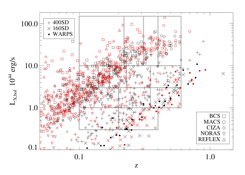
Figure 1.— Bolometric X-ray luminosity versus redshift for clusters in the eight cluster surveys used here. Bolometric X-ray luminosities are derived from $0.5-2.0$ keV ROSAT PSPC luminosities, assuming the $L_{\rm X}$ – $T$ relation of Markevitch (1998). Symbols for the cluster surveys are given in the legend. Red symbols denote clusters having an NVSS source projected within 250 kpc of the cluster center. The gray boxes mark the cells used to calculate average jet powers in §7.

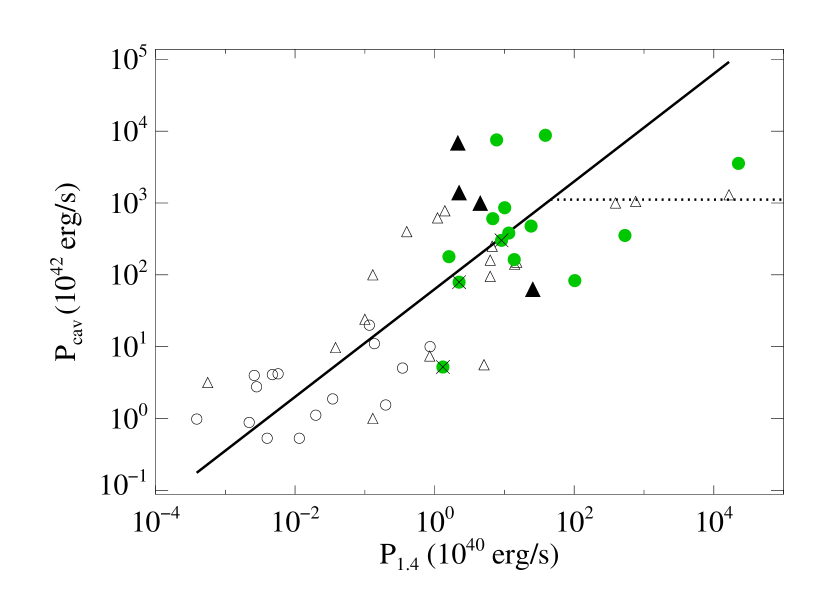
Figure 2.— Correlation between cavity power, $P_{\rm cav}$, estimated as $4pV/\tau$, and radio power, $P_{1.4}$. Clusters in our sample with known X-ray cavities are plotted as filled symbols. $P_{\rm cav}$ values for them are taken from Hlavacek-Larrondo et al. (2012a, filled green circles) and Bîrzan et al. (2008, filled black triangles). “Possible” cavities from the sample of Hlavacek-Larrondo et al. (2012a) are marked with a cross to indicate that they are less secure detections. Open triangles and circles denote other clusters used by Bîrzan et al. (2008) and Cavagnolo et al. (2010) respectively. The solid line is the scaling relation of Equation (1). The dotted line shows the saturation level discussed in §3.2.

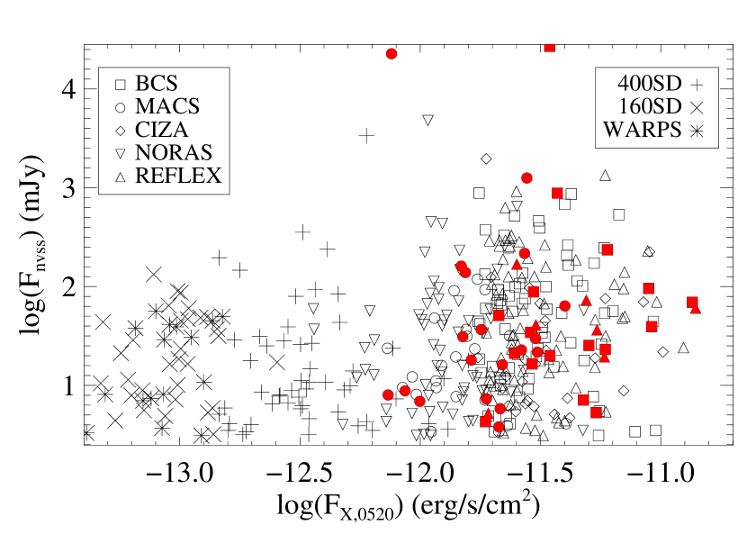
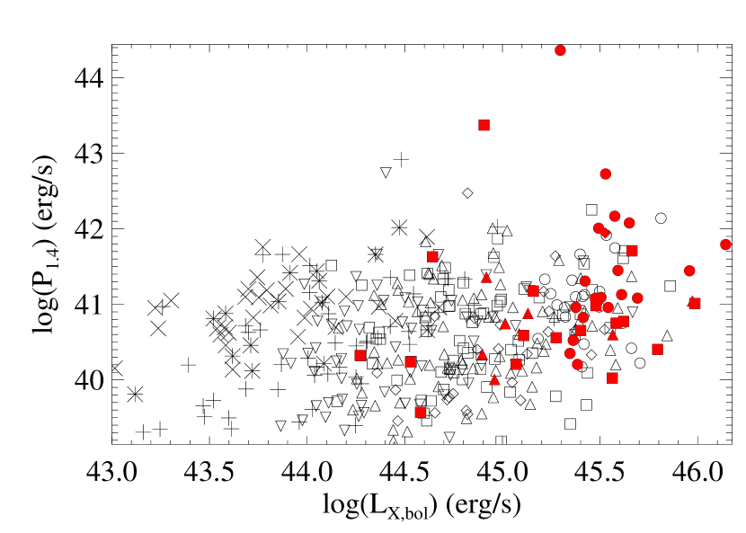
Figure 3.— Left: NVSS radio flux for AGN projected within 250 kpc of a cluster center versus 0.5 – 2 keV X-ray flux of the cluster. Right: Radio power at 1.4 GHz for the same sources versus bolometric X-ray luminosity of the host. Clusters identified as having strong cooling cores ($t_{\rm cool}<1$ Gyr) in Cavagnolo et al. (2009) are plotted in red. Most of the remaining clusters are not from the sample of Cavagnolo et al. (2009), so their cooling times are unknown.

3. The Sample

To extend the work of MMN11, we have combined eight major X-ray cluster surveys (Figure 1): the 400SD (Burenin et al., 2007), the 160 deg² Survey (160SD; Vikhlinin et al., 1998; Mullis et al., 2003), the Wide Angle ROSAT Pointed Survey (WARPS; Scharf et al., 1997; Horner et al., 2008), the MAssive Cluster Survey (MACS; Ebeling et al., 2001, 2007, 2010; Mann & Ebeling, 2012), the Brightest Cluster Survey (BCS; Ebeling et al., 1996, 2000), the Clusters in the Zone of Avoidance (CIZA; Ebeling et al., 2002; Kocevski et al., 2007), the Northern ROSAT All-Sky Cluster Survey (NORAS; Böhringer et al., 2000), and the ROSAT-ESO Flux Limited X-Ray Cluster Survey (REFLEX; Böhringer et al., 2001).

The first three surveys were compiled from serendipitously detected clusters in targeted ROSAT PSPC observations, while the other five cluster surveys are based on the ROSAT All Sky Survey catalogue (RASS; Voges et al., 1999). Many clusters are recorded in more than one of these surveys. These were identified by having centroid offsets of less than 2$\arcmin$. Most overlapping identifications are between the three serendipitous surveys, or NORAS and BCS. Of the 223 160SD clusters, 101 are included in 400SD, 40 of the 141 WARPS clusters are included in 400SD, and 213 of the 484 NORAS clusters are included in BCS. Redshifts for the overlapping entries are mostly consistent within 10% between catalogs. For the overlapping entries, we used the redshift, centroid, and X-ray luminosity from the highest priority survey. Priority order is as listed above, i.e. 400SD, 160SD, WARPS, MACS, BCS, CIZA, NORAS, and REFLEX. For the overlapping entries, the multiple redshift measurements of 18 clusters are inconsistent, with $|{\Delta z}/{z}|>10\%$. These clusters were excluded from our sample to ensure the accuracy of our redshifts and cluster identifications, although some measurement inconsistencies seem to have been resolved in the literature (see the summary in Piffaretti et al., 2011).

To combine the X-ray luminosity measurements from different surveys, we recalculated bolometric X-ray luminosities using the $L_{\rm X}-T$ relation from Markevitch (1998). The X-ray luminosities estimated from different entries for the same cluster were compared to examine the consistency of flux measurements in different surveys. The average difference in luminosity is about 10%. X-ray luminosities are used to estimate the number of particles in the clusters in §7 and so to derive the average AGN energy injected per particle. Because uncertainties in $P_{\rm{jet}}$ due to the scatter in the scaling relation of Equation (1) dominate in estimates of the average radio jet power, uncertainties in the X-ray luminosities are not an issue in this study.

Collectively, these eight X-ray cluster surveys contain 1032 clusters in the declination range $-38\arcdeg<\delta<68\arcdeg$, an area that is well covered by the NVSS. The background source density for the sample is $\rho_{\rm bkg}>35\,{\rm deg^{-2}}$. We focused on clusters in the redshift range 0.1 to 0.6. The upper redshift limit is set by limited sampling and the lower limit is set to avoid the complexity of radio flux measurements for resolved sources. After the redshift cuts, 685 clusters remain in the range of bolometric X-ray luminosities $3\times 10^{43}$ to $15\times 10^{45}$$\rm\,erg\,s^{-1}$.

3.1. Radio Sources in Clusters

Following the analysis in MMN11, we cross-matched the coordinates of the clusters with radio sources in the NVSS catalogue. For our sample of 685 clusters, 357 have NVSS radio sources above a flux limit of 3 mJy projected within 250 kpc. MMN11 (see also Lin & Mohr, 2007; Best et al., 2007) showed that the density of radio sources at the center of the clusters is much higher ($\sim 2$ Mpc^-2) than at larger radii ($0.3$ Mpc^-2), so the probability that these central sources are not associated with the clusters is small. The total expected number of background contaminated clusters is 25, i.e., $7\%$ of the 357 clusters. There is little to be gained from using a smaller aperture due to the large uncertainties in the cluster coordinates determined from ROSAT data (see MMN11 for a more detailed discussion based on 400SD clusters).

In Table 1, we show the number of clusters in each survey and the fraction of clusters with radio sources for two redshift ranges, $0.1<z<0.3$, and $0.3<z<0.6$. Here, the cluster samples are defined by the same criteria, i.e., declination range and NVSS background density, as the composite sample (see §3), but redundant entries for a cluster in the different surveys are not excluded. For the lower redshift range (column 3), the radio source fractions for the three serendipitous surveys, at $\simeq 32\%$, are consistently lower than those for the five all-sky surveys, which all exceed $55\%$. For the higher redshift range (column 6), the situation is similar, although the variations between the all-sky surveys are greater due to large statistical errors. These differences between the serendipitous and the all-sky surveys are probably due to the correlation between radio source fraction and the X-ray luminosity of a host cluster, since the clusters in the all-sky surveys are generally more luminous than those in the serendipitous surveys at a given redshift. This correlation is discussed in §5. In order to provide a fair comparison of radio source fractions at different redshifts, f_R,hif in column (4) is the fraction of clusters with a central radio source more powerful than $P_{1.4}=3.8\times 10^{40}$$\rm\,erg\,s^{-1}$, the power cut defined for the high redshift sample. Column (6) gives the same fraction for the higher redshift sample, showing that these fractions are marginally greater for the higher redshift range.

Table 1Fraction of clusters with NVSS sources

Survey	$0.1<\rm z<0.3$			$0.3<\rm z<0.6$
	Ncl	fR	fR,hif	Ncl	fR,hif
(1)	(2)	(3)	(4)	(5)	(6)
400SD	97	$0.32\pm 0.06$	$0.09\pm 0.03$	53	$0.25\pm 0.1$
160SD	80	$0.32\pm 0.07$	$0.21\pm 0.06$	63	$0.29\pm 0.1$
WARPS	55	$0.33\pm 0.09$	$0.16\pm 0.06$	47	$0.32\pm 0.1$
BCS	131	$0.55\pm 0.08$	$0.28\pm 0.05$	9	$0.44\pm 0.3$
MACS	0	$\cdots$	$\cdots$	65	$0.48\pm 0.1$
CIZA	35	$0.63\pm 0.17$	$0.29\pm 0.10$	2	$0$
NORAS	191	$0.55\pm 0.07$	$0.26\pm 0.04$	23	$0.13\pm 0.1$
REFLEX	122	$0.59\pm 0.09$	$0.31\pm 0.06$	7	$0.86\pm 0.5$

3.2. Cavity Powers

Some of our sample clusters were shown to have X-ray cavities by Hlavacek-Larrondo et al. (2012a) and Bîrzan et al. (2008). Figure 2 shows estimates of jet power, $P_{\rm cav}=4pV/\tau_{\rm buoy}$, for these, plotted against their radio powers, together with the scaling relation of Equation (1), and the remaining data of Bîrzan et al. (2008) and Cavagnolo et al. (2010) used to establish the scaling relation. The new data (filled green circles) are consistent with the scaling relation and their scatter is similar to that for the data used to establish the scaling relation.

The scaling relation (solid line) may be overestimating $P_{\rm{jet}}$ for the five powerful radio sources with $P_{1.4}\geq 10^{42}$$\rm\,erg\,s^{-1}$in Figure 2 (but see Daly et al., 2012, and Antognini et al. 2012). A similar result is seen in Figure 1 of Cavagnolo et al. (2010). This departure could arise if a significant fraction of their radio synchrotron power is generated by “hot spots” which are absent from the FR I radio sources that form most of the scaling relation (e.g., 3C295; Harris et al., 2000, Cygnus A; Wilson et al., 2006). This synchrotron flux should be excluded before applying the scaling relation. In some cases (e.g., Forman et al., 2005; Lal et al., 2010) shock fronts may also contribute significantly to the power deposited into hot atmospheres. In principle, the energy associated with shock fronts should also be taken into account when the $P_{\rm{jet}}$ is measured. However, high-quality X-ray data and careful data analysis are necessary to detect shock fronts and to estimate the associated energy, which would be a major undertaking for a large data set. For consistency, values of $P_{\rm cav}$ in Figure 2 were estimated using only the enthalpy and the cavity inflation time.

The number of powerful sources in Figure 2 is too small to place a strong constraint on the slope of the scaling relation at the high end. So it is unclear whether and to what degree we may be overestimating the jet power in these sources. However, this issue is crucial for to making reliable estimates of $P_{\rm{jet}}$ in §7. If the scaling holds, the mean power output of short-lived but powerful radio sources could rival the level of normal radio-AGN feedback over time. We therefore take two approaches to calculating the mean power. First, we excluded the most powerful radio sources, so that the resulting average cavity power places a lower limit on the true average cavity power. Second, we set $P_{\rm{jet}}$ for the powerful sources, assuming that the jet power saturates at the constant value of $P_{1.4}=2.4\times 10^{41}\,\rm\,erg\,s^{-1}$ for high radio powers, i.e, $P_{\rm{jet}}(P_{1.4}>2.4\times 10^{41}\,\rm\,erg\,s^{-1})=1.07\times 10^{45}$$\rm\,erg\,s^{-1}$(dashed line in Figure 2). The saturation level is set to the mean value of $\log\,P_{\rm cav}$ for the 5 most powerful radio sources in Figure 2. The two approaches are compared in §7.

3.3. Cooling Times

Central cooling times for 110 clusters in our sample were estimated using archival Chandra data for the “Archive of Chandra Cluster Entropy Profile Tables” project (ACCEPT; Cavagnolo et al., 2009). Briefly, Cavagnolo et al. (2009) fit annular spectra for each cluster to determine the cooling time as a function of the radius, assuming a profile for the cooling time of the form

$$t_{\mathrm{cool}}(r)=t_{c0}+t_{100}\left(\frac{r}{100\mbox{$\mathrm{~{}kpc}$}}\right)^{\alpha},$$ (2)

where $t_{c0}$ and $t_{100}$ are constants. The value for the central cooling time, $t_{c0}$, is the cooling time $t_{\mathrm{cool}}$ used in this paper.

4. Correlation Between Radio Power and X-ray Luminosity

The dependence of the power of a radio source on the X-ray luminosity of its hosting cluster is shown in Figure 3. As found by MMN11, the correlation is weak. The Kendall correlation coefficient for the fluxes is small, at $r=0.16$, although it differs from zero at high significance, the probability of getting a value this large by chance being only $1.1\times 10^{-4}$. The slope of the relationship between the fluxes is $d\log F_{\rm NVSS}/d\log F_{\rm X,0520}=0.28\pm 0.05$ and between the powers it is $d\log P_{1.4}/d\log L_{\rm X,bol}=0.33\pm 0.05$. The surprising agreement between these slopes requires a weak correlation between distance and luminosity for the sample (Figure 1). Since cluster X-ray luminosity increases with mass, it follows that the radio power of a central AGN in clusters is weakly dependent on the cluster mass.

Confining attention to clusters with cooling times shorter than 1 Gyr, plotted in red in Figure 3, the Kendall correlation coefficient for the fluxes is $r=0.3$, with a probability of $0.04$, still significant at the 95% level. For these clusters, $d\log F_{\rm NVSS}/d\log F_{\rm X,0520}=0.47\pm 0.50$ and $d\log P_{1.4}/d\log L_{\rm X,bol}=0.51\pm 0.30$. While there is marginal evidence that the radio power of a central AGN is more strongly dependent on the X-ray luminosity in these clusters, the correlation is weaker than expected from the work of Rafferty et al. (2006), who found a relationship between jet power and cooling rate in clusters. Several factors may be at work here. First, Rafferty et al. (2006) use cavity powers determined from X-ray data, a fairly diect measure, to estimate jet powers. Using Equation (1) to connect radio powers to jet powers injects significant extra scatter into the relationship between cavity power and cooling power. Second, the dynamic range of X-ray luminosities in Figure 3 is significantly smaller than that of the cooling powers in Rafferty et al. (2006), tending to bury any correlation in the scatter. Lastly, Rafferty et al. (2006) relate the cavity power to the power radiated within the cooling radius. If feedback is at work, the jet power should only depend on cooling in this region. Although X-ray emission from within the cooling radius can be an appreciable fraction of the total X-ray luminosity of a cluster, the correlation is diluted by X-ray emission from larger radii.

4.1. Distribution of Radio Powers for Cluster Central AGN

If AGN feedback prevents cooling and star formation in cluster central galaxies, then a high cooling rate implies a high AGN power; thus, the radio powers of strong cooling core clusters are expected to be greater.

In Figure 4, we compare distributions of radio power for the central AGN to examine whether the clusters with cooling cores or cavities do have greater radio powers. The red histogram in the upper left panel shows cooling core clusters, with $t_{\mathrm{cool}}<1$ Gyr from the ACCEPT data (Cavagnolo et al., 2009), while the blue histogram on the upper right shows non-cooling core clusters, with $t_{\mathrm{cool}}>3$ Gyr from the ACCEPT data. For comparison, the distribution for the entire cluster sample, selected as discussed in §3, is plotted in gray. The distribution of radio powers in non-cooling core clusters is broad, including some powerful radio sources, although the number of clusters with $t_{\mathrm{cool}}>3$ Gyr common to our sample and the ACCEPT sample is too small to provide a robust result. Further complicating matters, Rafferty et al. (2008) and Cavagnolo et al. (2008) found that radio AGN and star formation activity at cluster centers associated with cooling flows are triggered when the central cooling time falls below a threshold of $t_{\mathrm{cool}}\leq 0.5$ Gyr. Our X-ray data are generally unable to detect such a threshold, making the distinction between cooling-flows and non-cooling flows rather uncertain.

For a larger sample of non- or weak-cooling core clusters, radio powers for 400SD and 160SD clusters with $z>0.3$ are plotted in the cyan histogram of the lower right panel. The 400SD clusters at high redshifts were found to be dominated by non- or weak-cooling core clusters by Santos et al. (2010) and Samuele et al. (2011). Clusters in the 160SD and 400SD cluster samples should be similar because these two surveys used much the same selection criteria. To avoid bias due to the higher cut in radio power at higher redshifts, the gray shaded histogram shows all the clusters of our sample with $z>0.3$ for comparison. The means of the log of the radio power for these two samples are $\log P_{1.4}=40.98\pm 0.08$ for the 400SD and 160SD clusters and $\log P_{1.4}=41.07\pm 0.06$ for the whole sample, which are consistent with one another, showing no evidence of an offset between the two distributions.

Despite this, the most powerful radio sources in our sample do tend to be associated with cooling cores. The fraction of cooling core clusters with radio sources having $P_{1.4}>10^{42}$$\rm\,erg\,s^{-1}$is $13\pm 5\%$ (6/45), compared to $10\pm 7\%$ (2/19) for the non-cooling core clusters of the upper right panel and $3\pm 2\%$ (1/36) for the 160SD and 400SD samples in the lower right panel. In summary, radio sources in the cooling core clusters are generally as powerful as those in the non-cooling cores, apart from the most powerful radio sources. On the other hand, we have reliable estimates of the cooling rate for only a small sub-sample, and better coverage of deep and high resolution X-ray data are required for a more robust conclusion.

The green histogram in the lower left panel of Figure 4 shows radio powers for clusters identified with cavities by Hlavacek-Larrondo et al. (2012a), with clusters from our sample at $z>0.3$ for comparison. The clusters with cavities do have slightly greater radio powers (mean $\log P_{1.4}=41.55\pm 0.22$) than clusters in our sample (mean $\log P_{1.4}=41.07\pm 0.06$). Furthermore, the distribution of radio powers for the clusters with cavities has a longer tail at high powers. The fraction of these clusters having a powerful radio source ($P_{1.4}>10^{42}\rm\,erg\,s^{-1}$) is $30\pm 13\%$ (6/20), compared to $8\pm 3\%$ (8/96) for our sample.

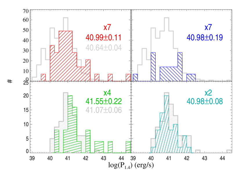
Figure 4.— Distributions of radio power. The panels show histograms of $P_{1.4}$ for various subsamples in different colors: red in the upper left panel for the cooling core clusters of Figure 3, blue in the upper right panel for non-cooling core clusters, i.e., those with cooling times greater than 3 Gyr, cyan in the lower right panel for 400SD and 160SD clusters at $z>0.3$, and green in the lower left panel for the clusters with cavities identified by Hlavacek-Larrondo et al. (2012a). The gray histogram in the two upper panels shows our entire sample, as described in §3, and the filled gray histogram in the lower two panels show clusters in our sample with $z>0.3$. The colored histograms are weighted by a factor noted in each panel to make comparisons easier. Biweight means and their $95\%$ confidence ranges are given in the same colors as the corresponding samples.

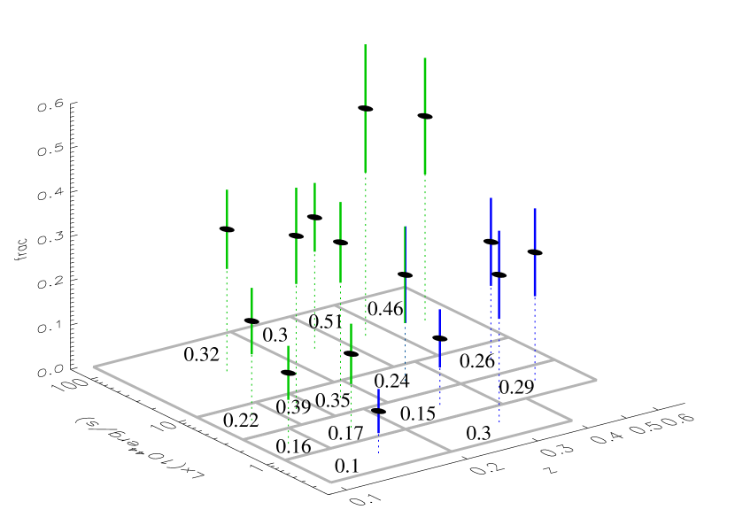
Figure 5.— Fraction of clusters having at least one NVSS source projected within 250 kpc of the cluster center. The NVSS sources are selected to have $P_{1.4}>3.8\times 10^{40}$$\rm\,erg\,s^{-1}$. The redshift and X-ray luminosity bins are defined in Figure 1. Colors are used to distinguish bins dominated by clusters from the all-sky surveys (green) from those from the serendipitous surveys (blue). Error bars show uncertainties calculated assuming Poisson statistics. The fraction for each bin is noted in the bin.

5. Fraction of Clusters with Radio AGN

MMN11 found that the probability of a more luminous and higher-redshift 400SD cluster hosting an AGN is marginally higher than that for a less luminous and lower-redshift 400SD cluster, at the $1\sigma$ level. In their relatively small sample, redshifts and X-ray luminosities are coupled, so that the more luminous clusters also have higher redshifts. With our larger composite sample, we can examine separately how the fraction of clusters matched with NVSS radio sources depends on the X-ray luminosity and redshift, as shown in Figure 5. For computing radio source fractions here, radio sources are defined as having powers, $P_{1.4}>3.8\times 10^{40}$$\rm\,erg\,s^{-1}$, corresponding to a radio flux of 2 mJy for a source at $\rm z=0.6$. The fraction of clusters having a radio source is computed for each bin defined in Figure 1. From the figure, the fraction generally increases with both the redshift and the X-ray luminosity of a cluster.

A significant concern is that trends in the radio fraction can be masked by differences between the serendipitous and all-sky surveys. For example, for the four redshift bins bounded by $z=0.14,0.17,0.23,0.35$, and 0.6, in the luminosity range $3<L_{\rm X}/10^{44}\rm\,erg\,s^{-1}<10$, the fractions of radio sources in the two lower redshift bins, $0.14<z<0.23$, which are dominated by clusters from the all-sky surveys, are higher than the fractions for the two higher redshift bins, which are dominated by clusters from the serendipitous surveys. This concern is related to the persistent question of whether the serendipitous surveys preferentially select non-cooling core clusters, while the all-sky surveys favor cooling core clusters (cf. Vikhlinin et al., 2006; Eckert et al., 2011). Under AGN feedback models, cooling core clusters are more likely to host central radio AGN (e.g., Rafferty et al., 2006; Cavagnolo et al., 2008). However, even if the serendipitous and all-sky surveys differ, Figure 5 suggests that this does not mask an increasing trend in the radio fraction with redshift and luminosity among the higher-redshift and more luminous clusters. This trend can be seen separately in the blue and green points that are dominated by serendipitous and all-sky surveys, respectively.

Figure 6 shows average radio powers per cluster for the bins of Figure 1. As for Figure 5, a threshold on the radio power of $P_{1.4}>3.8\times 10^{40}$$\rm\,erg\,s^{-1}$ was used to avoid spurious redshift dependence in the results. The three most powerful radio sources in our sample, 3C 295, Hercules A, and 3C 288, are excluded from the averages, since they are so dominant that they would obscure the underlying trends. Thus, the average radio powers in Figure 6 are lower limits.

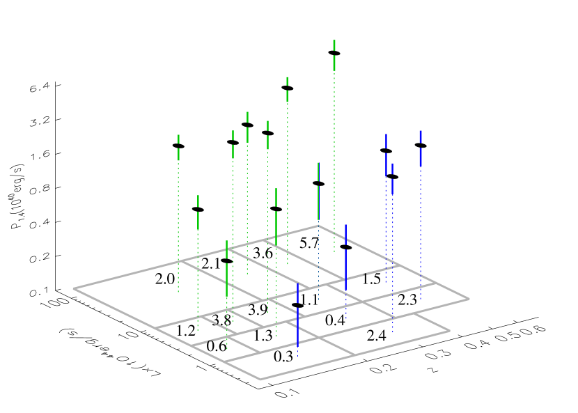
Figure 6.— Average radio power for sources projected within 250 kpc of cluster centers. Radio sources are selected from the NVSS, above a radio power of $P_{1.4}>3.8\times 10^{40}$$\rm\,erg\,s^{-1}$ for all redshifts. The average radio power is recorded in each bin. Colors have the same meaning as in Figure 5.

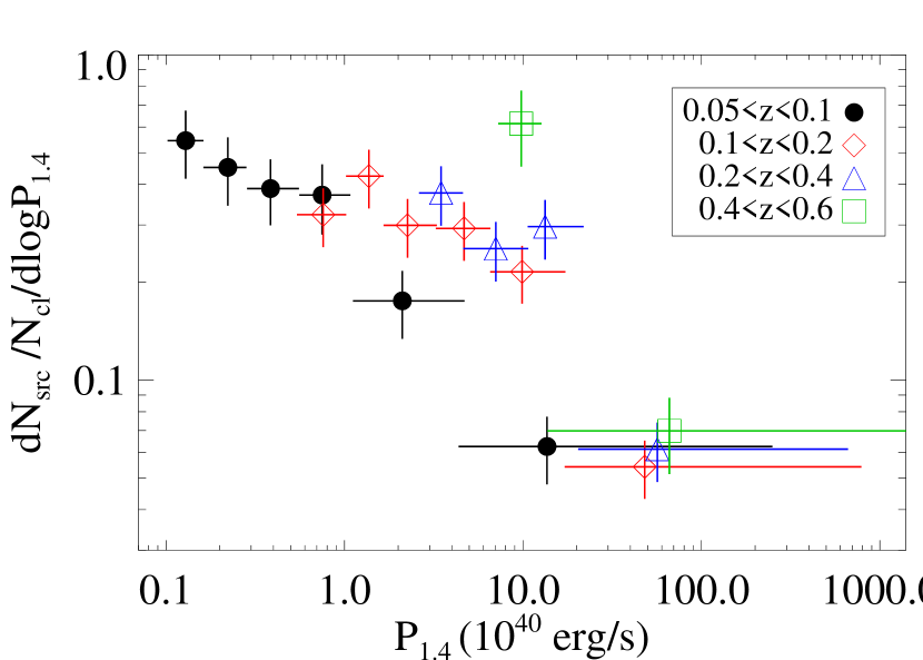
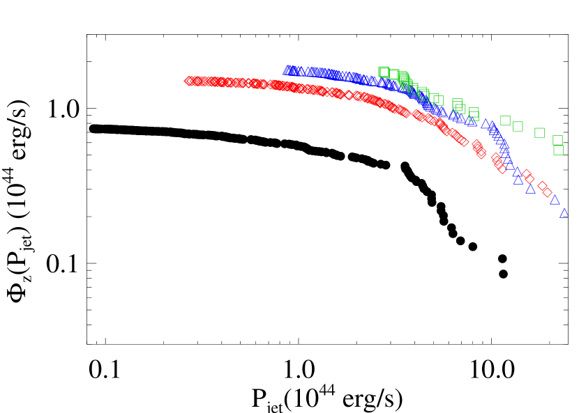
Figure 7.— Left: Mean number of radio sources per cluster, per $\log P_{1.4}$ as a function of NVSS radio power, $P_{1.4}$. Right: Cumulative jet power per cluster for radio jets more powerful than $P_{\rm{jet}}$. Details are given in §6. Both functions are calculated for the four redshift ranges listed in the legend of the left panel.

6. Evolution of Number and Power of Cluster Central Radio Sources

The distribution of the number of radio sources per cluster, per unit $\log P_{1.4}$ is

$$\varphi(P_{1.4})={1\over N_{\rm cl}}{dN_{\rm src}(>P_{1.4})\over d\log P_{1.4}},$$ (3)

where $N_{\rm src}(>P_{1.4})$ is the number of radio sources with powers greater than $P_{1.4}$ in the cluster population of interest and $N_{\rm cl}$ is the number of clusters in the population. The expected number of background radio sources for each cluster is subtracted from $N_{\rm src}$ and there may be more than one radio source in a cluster. Note that, since the normalization of $\varphi$ gives the mean number of radio sources per cluster it may be greater than unity. The distribution $\varphi(P_{1.4})$ is plotted in the left panel of Figure 7 for clusters in the four redshift ranges, $0.05-0.1-0.2-0.4-0.6$. Following §3, only clusters with luminosities in the range $3\times 10^{43}<L_{\rm X}<15\times 10^{45}$$\rm\,erg\,s^{-1}$ are included. Values for $\varphi(P_{1.4})$ are shown only for powers above a threshold corresponding to the flux limit of 3 mJy for the redshifts $z=0.1,0.2,0.4$, and 0.6. The distribution, $\varphi(P_{1.4})$, increases with redshift, evolving more significantly at the higher power end, consistent with previous findings (e.g., Galametz et al., 2009; Hart et al., 2011).

Closely related to $\varphi(P_{1.4})$, we define $\phi(P_{\rm{jet}})$, the number of radio jets per cluster per unit $\log P_{\rm{jet}}$, by replacing the radio power $P_{1.4}$ in Equation (3) with $P_{\rm{jet}}$ calculated from Equation (1),

$$\phi(P_{\rm{jet}})={1\over N_{\rm cl}}{dN_{\rm src}(>P_{\rm{jet}})\over d\log P_{\rm jet}}.$$ (4)

The cumulative jet power per cluster from jets more powerful than $P_{\rm{jet}}^{\rm lim}$ is then

$$\Phi_{z}(P_{\rm{jet}}^{\rm lim})=\int_{P_{\rm{jet}}^{\rm lim}}^{\infty}\phi(P_{\rm{jet}})P_{\rm{jet}}\,d\log P_{\rm{jet}}.$$ (5)

This is plotted as a function of $P_{\rm{jet}}^{\rm lim}$ in four redshift ranges in the right panel of Figure 7. Here and earlier in Equation (3), $d\log P$ is calculated as the Voronoi interval for the power of each radio source, although, for $\varphi(P_{1.4})$, the data are binned in $P_{1.4}$. Values are plotted only for $P_{\rm{jet}}^{\rm lim}$ above a lower limit corresponding to the radio flux limit of 3 mJy for the different redshift ranges.

6.1. Correcting for the Radio Flux Limit

A fair comparison of the average $P_{\rm{jet}}$ per cluster for different redshifts requires that we use the same value of $P_{\rm{jet}}^{\rm lim}$. For the whole sample, that would limit us to using the jet power corresponding to the radio power cutoff for $z=0.6$. This is very restrictive and it would mean discounting the power input of many less powerful radio sources seen at lower redshifts. Alternatively, we can estimate the average jet power for smaller values of $P_{\rm{jet}}^{\rm lim}$ by applying a correction factor $w$, calculated from the form of $\Phi_{z}$ at lower redshifts, on the assumption that the shape of $\Phi_{z}(P_{\rm{jet}}^{\rm lim})$ does not evolve with $z$. This assumption is supported by studies of the evolution of the radio luminosity function in, e.g., Clewley & Jarvis (2004), Sadler et al. (2007), Sommer et al. (2011), and Simpson et al. (2012), which find mild evolution of radio galaxies with $P_{1.4}<10^{41}$ erg/s. It gives the correction factor

$$w(z)=\frac{\Phi_{z_{0}}[\tilde{P}^{\rm lim}_{\rm jet}(z_{0})]}{\Phi_{z_{0}}[\tilde{P}^{\rm lim}_{\rm jet}(z)]}.$$ (6)

where $\tilde{P}^{\rm lim}_{\rm jet}(z)$ is the lower limit on the jet power for redshift $z$, which is obtained by inserting the radio power corresponding to the flux limit of 3 mJy at redshift $z$ into Equation (1). The cumulative jet power, $\Phi_{z_{0}}$, used for reference here is that for the redshift range of $0.05<z<0.1$. For example, for the redshift bin $0.4<z<0.6$ the correction factor is $w(z\simeq 0.5)=1.6$, calculated for $\tilde{P}^{\rm lim}_{\rm jet}(z)=2.4\times 10^{44}$$\rm\,erg\,s^{-1}$ and $\tilde{P}^{\rm lim}_{\rm jet}(z_{0})=8.6\times 10^{42}$$\rm\,erg\,s^{-1}$. The correction factor, $w(z)$, is used in the calculation of the average jet powers below.

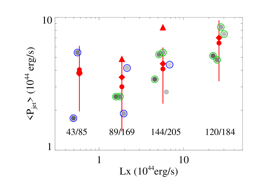
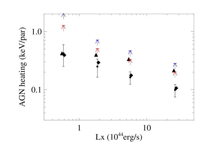
Figure 8.— Upper panel: Mean jet power $\langle P_{\rm{jet}}\rangle$ vs. X-ray luminosity. Gray circles correspond to the bins in $z$ and $L_{\rm X}$ shown in Figure 1. For each range of $L_{\rm X}$, darker shades of gray correspond to lower redshift bins. The red points with uncertainties are time averaged values, $\langle P_{\rm{jet}}\rangle_{\rm int}$, for the same ranges of $L_{\rm X}$ as the gray points. The number of clusters hosting NVSS sources and the total numbers of clusters is given at the bottom of the panel for each range of $L_{\rm X}$. Lower panel: Average AGN energy injected per particle. The filled circles with error bars give the average energy per particle injected by radio jets, integrated over the redshift ranges marked in Figure 1. Jet powers are calculated from Equation (1), excluding the most powerful radio sources with $P_{1.4}\geq 10^{42}$$\rm\,erg\,s^{-1}$. The impact of the jets is extrapolated to $z=2$ using two models: constant mean jet power (red arrows) and the linear evolution of $P_{\rm{jet}}$ discussed in §6 (blue arrows). The effect of including $P_{\rm{jet}}$ for the most powerful radio sources is also shown, calculated using the saturated scaling relation as diamonds and the scaling relation of Equation (1) as triangles.

7. Average Jet Power

The average jet powers, $\langle P_{\rm{jet}}\rangle$, shown in the upper panel of Figure 8 were estimated using a Monte Carlo method that accounts for the uncertainties in the radio fluxes and the parameters in Equation (1), the distribution of radio spectral indices, and the large intrinsic scatter ($\sigma_{1.4}$) in the relation of Equation (1). Note that the log of the arithmetic mean of $P_{\rm{jet}}$ for a lognormal distribution is greater than the “mean” of its log that is given by Equation (1). For each range of $L_{\rm X}$, the redshift bins of Figure 1 are chosen to distribute the clusters evenly between the bins. First, $\langle P_{\rm{jet}}\rangle$ is calculated for each bin in Figure 1, then this is integrated over time for a given range of $L_{\rm X}$ to give the time averaged mean jet power

$$\langle P_{\rm{jet}}\rangle_{\rm int}=\frac{\sum_{i}\left[\langle P_{\rm jet}(z_{i},L_{\rm X})\rangle{w_{z_{i}}}{t_{{z}_{i}}}\right]}{\sum_{i}t_{z_{i}}},$$ (7)

where $t_{z_{i}}$ is the time interval for redshift bin $i$ and $w_{z_{i}}$ is the correction factor calculated from Equation (6). The full redshift range is 0.1 to 0.4 for the lowest range of $L_{\rm X}$ and 0.1 to 0.6 for the remainder. In the bins for each range of $L_{\rm X}$, the evolution of $P_{\rm{jet}}$ seen in the right panel of Figure 7 is overwhelmed by the large uncertainties, particularly from the scatter in the relation of Equation (1). Because of this, possible differences between the serendipitous and all-sky surveys discussed in §5 are a minor issue.

In MMN11, we concluded that $\langle P_{\rm{jet}}\rangle$ shows no significant dependence on $L_{\rm X}$. However, the limited sample size prevented isolation of $L_{\rm X}$ from the redshift, because the most luminous clusters in the 400SD sample are at higher redshifts. Using the larger cluster sample here, we can break this degeneracy and estimate the $\langle P_{\rm{jet}}\rangle$ for clusters with different X-ray luminosities over the redshift range $0.1<z<0.6$ and the upper panel of Figure 8 shows that the mild increase of $\langle P_{\rm{jet}}\rangle$ with X-ray luminosity is not significant, consistent with other findings (Gaspari et al., 2011; Antognini et al., 2012). Since $\langle P_{\rm{jet}}\rangle$ is similar for all clusters, regardless of their X-ray luminosities, the energy input per particle from AGN is larger in less massive clusters (see also Best et al., 2007; Giodini et al., 2010, MMN11).

Using the $L_{\rm X}$ – $M_{500}$ relation of Vikhlinin et al. (2009) and a gas mass fraction of $0.12$, we can estimate the average gas mass within $R_{500}$, $\langle M_{\rm gas}\rangle$, for each luminosity range in the upper panel of Figure 8. Integrating the jet power over time (cf. Equation 7), gives the mean energy injected into clusters by radio AGN. Therefore, the mean total energy per particle injected by the radio sources is

$${\rm E}_{\rm jet}=\frac{\langle P_{\rm{jet}}\rangle_{\rm int}\,t_{z,\rm int}{\mu}m_{\rm p}}{\langle M_{\rm gas}\rangle},$$ (8)

where $\mu=0.59$ is the mean molecular weight, $m_{\rm p}$ is the proton mass and $t_{z,\rm int}=\sum_{i}t_{z_{i}}$. Here, the integration time is limited to correspond to the redshift ranges for the sample bins. In principle, the energy injected by the radio sources should be traced back to the time when BCGs formed ($z\sim 2$, e.g., van Dokkum & Franx, 2001). Even with no AGN evolution, extending the integration back to $z=2$ boosts the energy injected per particle substantially (red arrows in Figure 8) over the values for the redshift range of the sample (small dots). This estimate is conservative, because AGN are more active in the past (e.g., Galametz et al., 2009; Martini et al., 2009) and the clusters have assembled from smaller systems that may well have contained more than one BCG. To allow for the evolution of the $P_{\rm{jet}}$  Equation (8) can be generalized to

$${\rm E}_{\rm jet}=\int\frac{{\mu}m_{\rm p}}{\langle M_{\rm gas}\rangle}\langle P_{\rm{jet}}\rangle_{\rm int}\,dt,$$ (9)

where we assume that ${\langle M_{\rm gas}\rangle}$ does not depend on the time. The evolution of the cumulative $P_{\rm{jet}}$ (Figure 7 right) is modeled using a simple linear function,

$$\langle P_{\rm{jet}}\rangle_{\rm int}\sim\Phi_{z}(P_{\rm{jet}})\sim{\rm A+B}t,$$ (10)

where the parameters (A, B) are fitted to $\Phi_{z(t)}(P_{\rm{jet}})$ from Equation (5) for $z(t)=[0.15,0.3,0.5]$, and $P_{\rm{jet}}=3\times 10^{44}$$\rm\,erg\,s^{-1}$. This model raises the total energy input by another factor of $50\%$ (blue arrows in Figure 8). Note that our linear evolution model neglects the uncertainty in the correlation.

We discuss the interpretation of Figure 8 in the next section, §8. In short, the average AGN energy input to the clusters with luminosities of $0.3<L_{X}({\rm 10^{44}\,erg\,s^{-1}})<1.0$ can reach 1.3 – 2 keV/particle for ICM within $R_{500}$, depending on the details of AGN evolution. For the most massive clusters, with X-ray luminosities of $L_{X}>10^{45}$$\rm\,erg\,s^{-1}$, the average AGN input energy is also significant, at 0.2 to 0.3 keV/particle. Note that the energy input of the single AGN outburst in the MS0735+7421 cluster is $\sim 0.25$ keV per particle within the central 1 Mpc (Gitti et al., 2007). It is therefore plausible that a single, powerful AGN outburst can rival the integrated AGN energy input over time.

8. Discussion

8.1. AGN Energy Input

A few points need to be addressed regarding the results in Figure 8. First, the average jet powers are affected disproportionately by the most powerful radio sources, which are the least likely to be background sources. As shown in the lower panel of Figure 8, the average AGN energy deposited per particle for X-ray luminous clusters would be boosted by a factor of two assuming the scaling relation Equation (1) holds for the few sources with $P_{1.4}>10^{42}$$\rm\,erg\,s^{-1}$. This would imply that a single, powerful radio AGN can be as important to heating atmospheres as the integrated power output of radio sources over time. As discussed in section 3.2, Equation (1) may be overestimating the $P_{\rm{jet}}$ for the few powerful sources with $P_{1.4}>10^{42}$$\rm\,erg\,s^{-1}$in Figure 2. The saturated scaling relation gives average jet powers including all radio sources (diamonds) that differ little from those obtained when the powerful radio sources are excluded (circles). If the scaling relation does saturate, the small offsets between the spheres and diamonds in the lower panel of Figure 8 show that excluding the most powerful sources makes little difference to the mean jet power estimates.

On the other hand, our assumption that the cluster masses ($M_{500}$) remain constant for the calculation of the mean energy injected per particle fails to consider the hierarchical assembly of clusters. Allowing for cluster growth, Hart et al. (2011) demonstrated that jet power from central radio AGN in clusters could increase by a factor of 10 per particle from $z=0.2$ back to 1.1. At earlier times, AGN jets are more powerful and cluster progenitors are less massive. The long term effect of preheating of these early radio AGN should be considered (e.g. Rawlings & Jarvis, 2004; Shabala et al., 2011). Therefore, the energy from radio jets accumulates more quickly per ICM particle in the building blocks of present day clusters. As less massive clusters assemble to form more massive ones, most of the excess energy is preserved. By ignoring this effect, we have certainly underestimated the total AGN energy accumulated in the ICM of massive clusters over their histories. One effect that might counteract this is that radio jets could break out of the atmospheres of less massive halos (e.g., the poorly confined sample of Cavagnolo et al., 2010), allowing some jet energy to escape. However, the huge mass of gas that will form the atmosphere of an incipient cluster is present from the outset and very few jets can escape from that. Jet energy escaping from a smaller atmosphere will be deposited in surrounding gas that is fated to collapse into the cluster. Unless the energy deposited by a jet is sufficient to unbind this gas from the cluster, it inevitably collapses into the cluster at some later time, carrying the excess energy along with it (apart from energy lost to radiation).

Our calculations ignore energy lost from the ICM by X-ray radiation. If we are interested in the net energy gain from radio jets, this must be taken into account. On the face of it, the upper panel of Figure 8 shows that the X-ray power radiated by the clusters in our sample exceeds the average power input from the central AGN for $L_{\rm X}\gtrsim 3\times 10^{44}\rm\,erg\,s^{-1}$. Our estimates of the mean jet power are conservative and only include central radio sources (projected within 250 kpc), when other radio sources may augment the total energy input significantly (Stocke et al., 2009). Nevertheless, it is likely that the ICM of the most luminous clusters suffers a net energy loss. It should be borne in mind that most of the X-ray power radiated by the great majority of clusters does not originate from a cooling core. Outside cooling cores it will take a very long time for the energy loss to have any noticeable impact. Central cooling times are available in the ACCEPT database (Cavagnolo et al., 2009) for only 110 members of our sample, leaving us poorly placed to examine the net effect of jets on cooling core clusters. Notably, Figure 8 shows that, even with our conservative estimates for the energy input from central radio jets, clusters less luminous than $L_{\rm X}\simeq 3\times 10^{44}\rm\,erg\,s^{-1}$ see a net energy gain. Thus, energy injected by central radio AGN accumulates in lower mass clusters, so that the integrated energy gain shown in the lower panel of the figure is mostly retained in these systems and has a significant impact on the ICM.

As discussed in §5, our sample shows increases in the fraction of clusters with central radio AGN for increases in both the X-ray luminosity and the redshift (Figure 5). It is, therefore, surprising that we do not see a more pronounced increase in the mean jet power with X-ray luminosity in the upper panel of Figure 8. The primary cause of this is the large scatter introduced by using Equation (1) to convert radio powers to jet powers. There is good reason to believe that mean jet powers do increase with cluster luminosities (e.g., Bîrzan et al., 2004; Rafferty et al., 2006; Sun, 2009, but see Antognini et al. (2012), Lin & Mohr (2007)). However, the modest increase is buried by the scatter in the $P_{1.4}-P_{\rm{jet}}$ relation. It is clearly desirable to find a more accurate way to estimate jet powers.

8.2. Supermassive Black Hole Growth

The integrated power output from radio-AGN at the centers of clusters over the past $\simeq 10$ Gyr implies substantial supermassive black hole growth. We have estimated the accreted mass required to fuel AGN from the integrated AGN power output over time. We assume a conversion efficiency between accreted mass and mechanical jet power of $\eta=0.1$, where $P_{\rm jet}=\eta\dot{M}c^{2}$, and we ignore radiation loses. We note that, although $\eta=0.1$ is commonly used in literature, the distribution of $\eta$ is an open issue (for a more detailed discussion, see Martínez-Sansigre & Rawlings, 2011). In some accretion models (e.g. Benson & Babul, 2009), $\eta$ approaches unity at high black hole spin. However, many estimates of $\eta$ (e.g. Churazov et al., 2005; Merloni & Heinz, 2008; Gaspari et al., 2012) suggest a small $\eta$, with $\eta=0.1$ near the upper limit of reasonable values for the jet efficiency. If the average efficiency is lower, the nuclear black holes need to grow even more to power these radio sources. Integrating the AGN mechanical energies shown in the bottom panel of Figure 8 over $5.7$ Gyr ($z=0.6$) gives an average accreted mass of $2-5\times 10^{8}M_{\odot}$ per supermassive black hole. Extrapolating back to $z=2.0$ over a look-back time of about $10.5$ Gyr, and assuming the modestly rising AGN power discussed earlier, implies an average increase of $6-14\times 10^{8}M_{\odot}$ per supermassive black hole. Note that, in hierarchically assembling clusters, this mass may be distributed among several black holes. These values are comparable to the black hole masses of BCGs inferred from black hole scaling relations (e.g. Lauer et al., 2007), which are thought to have been imprinted during the quasar era. Our result implies that normal AGN maintained over time by hot atmospheres may be as important to supermassive black hole growth in BCGs as earlier and, presumably, much more rapid formation processes (see the review in Merloni & Heinz, 2012). It is conceivable that normal radio-AGN activity may give rise to black hole masses in excess of the mass expected from the $M_{\rm BH}$–$\sigma$ relation for BCGs (Lauer et al., 2007). Furthermore, if $\eta$ indeed lie well below 0.1, the inferred black hole growth rates may be even larger, leading to the possibility of growing ultramassive black holes in BCGs (e.g., McNamara et al., 2009; Hlavacek-Larrondo et al., 2012b).

9. Summary

We have combined eight surveys of X-ray clusters to compile a composite sample with 1032 clusters located in the area covered by the NVSS. For each NVSS radio source projected within 250 kpc of a cluster center, we have estimated the mechanical power of its radio jet using the scaling relation, Equation (1), from Cavagnolo et al. (2010). The jet power is weakly correlated with the X-ray luminosity of a hosting cluster, but the most powerful radio sources, with $P_{1.4}>1.4\times 10^{42}$$\rm\,erg\,s^{-1}$, are all located in massive, cooling core clusters. The correlation is stronger if only the strong cooling core clusters with $t_{\mathrm{cool}}<1$ Gyr are considered. We have also examined the distribution of radio source powers in cooling and non-cooling core clusters, using values of $t_{\mathrm{cool}}$ from the ACCEPT project (Cavagnolo et al., 2009). Based on the modest number of our sample clusters in the ACCEPT database, radio sources in non-cooling core clusters are, in general, as powerful as those in cooling core clusters, except that the most powerful sources mostly appear in cooling cores.

We have examined both the average radio power of clusters and the fraction of clusters with radio sources. The cluster sample is large enough to separate the dependence of the radio source fraction on redshift and cluster X-ray luminosity and we find that it increases moderately with both. The average power is also larger in more massive clusters and at higher redshifts.

Finally, we have calculated the average AGN jet power using the scaling relation in Equation (1) (Cavagnolo et al., 2010). This overestimates $P_{\rm{jet}}$ for the few powerful radio sources in our sample with $P_{1.4}\geq 10^{42}$$\rm\,erg\,s^{-1}$, so that the average jet power would be dominated by these extremely powerful sources. Two approaches were used to solve this problem. In the first approach, the most powerful sources were simply excluded from the calculations, giving a lower limit on the average jet power. In the second approach, $P_{\rm{jet}}$ for the powerful radio sources was determined using a saturated version of the scaling relation, with the saturation level set empirically and saturated jet power based on the cavity powers of the five most powerful sources in our sample. The average jet powers determined using these two approaches are similar. In the upper panel of Figure 8, the average jet power is plotted against the cluster X-ray luminosity. Although the average jet power for the most luminous clusters is higher than for less luminous clusters, large uncertainties in their estimation make the differences insignificant. In general, the average jet power exceeds $3\times 10^{44}$$\rm\,erg\,s^{-1}$  even in the least luminous clusters, with $0.3<L_{\rm X}<1\times 10^{44}$$\rm\,erg\,s^{-1}$. Thus, the average jet power exceeds the radiation output of the least massive sample clusters by an order of magnitude.

The average jet power was integrated to redshift $z=2.0$ using two simple evolutionary models for the radio sources. For the first model, the radio power was taken to be constant and then the average AGN energy injected by jets exceeds 1 keV per particle in the least luminous clusters, with $0.3<L_{\rm X}<1\times 10^{44}$$\rm\,erg\,s^{-1}$, and $\simeq 0.2$ keV per particle in the most luminous clusters, with $L_{\rm X}>10^{45}$$\rm\,erg\,s^{-1}$. Here, the number of gas particles was calculated using the gas mass within $R_{500}$, determined from the $L_{X}-M_{500}$ relation. For the second model, the average jet power was taken to be a linear function of the cosmic time and then, integrating to $z=2.0$, the AGN energy input amounts to $\simeq 2$ keV per particle for clusters with $0.3<L_{\rm X}<1\times 10^{44}$$\rm\,erg\,s^{-1}$and $\simeq 0.3$ keV per particle for clusters with $L_{\rm X}>10^{45}$$\rm\,erg\,s^{-1}$.

Existing X-ray data for our sample are inadequate to distinguish the energy radiated by gas that would be significantly affected by radiative cooling. However, the total radiation output of the less massive clusters is small compared to the energy input from AGN. If the energy injected by AGN is stored in these systems, we estimate that the AGN energy injected since $z=2.0$ is significant for preheating of clusters. If so, rather than preheating, the effect of the AGN would be better described as “continual heating.” In carrying out these calculations, we have ignored the hierarchical assembly of clusters by assuming that the cluster masses are fixed. Since massive clusters assembled from less massive clusters, where the jet power per particle is larger, we expect that our estimates of the total AGN energy accumulated in massive clusters are low. We conclude that continual AGN energy input in the “radio mode” could well provide $>1$ keV per particle in less massive clusters, which approaches the excess energy required to account for observed departures from the self-similar scaling relations that would be expected otherwise (Wu et al., 2000).

Lastly, we have estimated the mass that was accreted by supermassive black holes in BCGs to fuel their radio AGN and power their jets. Assuming that the jet power is related to the accretion rate by $P_{\rm jet}=0.1\dot{M}c^{2}$, for a typical BCG in our sample, the nuclear black hole would have grown by about $10^{9}M_{\odot}$ since $z=2$. This is comparable to black hole masses for BCGs estimated by Lauer et al. (2007), implying that that the fueling of radio AGN at the centers of hot atmospheres may be as significant as the earlier quasar era for the growth of supermassive black holes in BCGs.

References

- Antognini et al. (2012) Antognini, J., Bird, J., & Martini, P. 2012, ApJ, 756, 116
- Arnaud & Evrard (1999) Arnaud, M., & Evrard, A. E. 1999, MNRAS, 305, 631
- Benson & Babul (2009) Benson, A. J., & Babul, A. 2009, MNRAS, 397, 1302
- Best et al. (2007) Best, P. N., von der Linden, A., Kauffmann, G., Heckman, T. M., & Kaiser, C. R. 2007, MNRAS, 379, 894
- Bîrzan et al. (2008) Bîrzan, L., McNamara, B. R., Nulsen, P. E. J., Carilli, C. L., & Wise, M. W. 2008, ApJ, 686, 859
- Bîrzan et al. (2004) Bîrzan, L., Rafferty, D. A., McNamara, B. R., Wise, M. W., & Nulsen, P. E. J. 2004, ApJ, 607, 800
- Böhringer et al. (2000) Böhringer, H., et al. 2000, ApJS, 129, 435
- Böhringer et al. (2001) —. 2001, A&A, 369, 826
- Bower et al. (2006) Bower, R. G., Benson, A. J., Malbon, R., Helly, J. C., Frenk, C. S., Baugh, C. M., Cole, S., & Lacey, C. G. 2006, MNRAS, 370, 645
- Burenin et al. (2007) Burenin, R. A., Vikhlinin, A., Hornstrup, A., Ebeling, H., Quintana, H., & Mescheryakov, A. 2007, ApJS, 172, 561
- Cavagnolo et al. (2008) Cavagnolo, K. W., Donahue, M., Voit, G. M., & Sun, M. 2008, ApJL, 683, L107
- Cavagnolo et al. (2009) —. 2009, ApJS, 182, 12
- Cavagnolo et al. (2010) Cavagnolo, K. W., McNamara, B. R., Nulsen, P. E. J., Carilli, C. L., Jones, C., & Bîrzan, L. 2010, ApJ, 720, 1066
- Churazov et al. (2005) Churazov, E., Sazonov, S., Sunyaev, R., Forman, W., Jones, C., & Böhringer, H. 2005, MNRAS, 363, L91
- Clewley & Jarvis (2004) Clewley, L., & Jarvis, M. J. 2004, MNRAS, 352, 909
- Condon et al. (1998) Condon, J. J., Cotton, W. D., Greisen, E. W., Yin, Q. F., Perley, R. A., Taylor, G. B., & Broderick, J. J. 1998, AJ, 115, 1693
- Croton et al. (2006) Croton, D. J., et al. 2006, MNRAS, 365, 11
- Daly et al. (2012) Daly, R. A., Sprinkle, T. B., O’Dea, C. P., Kharb, P., & Baum, S. A. 2012, MNRAS, 423, 2498
- Dunn & Fabian (2006) Dunn, R. J. H., & Fabian, A. C. 2006, MNRAS, 373, 959
- Dunn et al. (2005) Dunn, R. J. H., Fabian, A. C., & Taylor, G. B. 2005, MNRAS, 364, 1343
- Ebeling et al. (2007) Ebeling, H., Barrett, E., Donovan, D., Ma, C.-J., Edge, A. C., & van Speybroeck, L. 2007, ApJ, 661, L33
- Ebeling et al. (2000) Ebeling, H., Edge, A. C., Allen, S. W., Crawford, C. S., Fabian, A. C., & Huchra, J. P. 2000, MNRAS, 318, 333
- Ebeling et al. (2001) Ebeling, H., Edge, A. C., & Henry, J. P. 2001, ApJ, 553, 668
- Ebeling et al. (2010) Ebeling, H., Edge, A. C., Mantz, A., Barrett, E., Henry, J. P., Ma, C. J., & van Speybroeck, L. 2010, MNRAS, 407, 83
- Ebeling et al. (2002) Ebeling, H., Mullis, C. R., & Tully, R. B. 2002, ApJ, 580, 774
- Ebeling et al. (1996) Ebeling, H., Voges, W., Böhringer, H., Edge, A. C., Huchra, J. P., & Briel, U. G. 1996, MNRAS, 281, 799
- Eckert et al. (2011) Eckert, D., Molendi, S., & Paltani, S. 2011, A&A, 526, 79
- Evrard & Henry (1991) Evrard, A. E., & Henry, J. P. 1991, ApJ, 383, 95
- Fabian (1994) Fabian, A. C. 1994, ARAA, 32, 277
- Fabian et al. (2006) Fabian, A. C., Sanders, J. S., Taylor, G. B., Allen, S. W., Crawford, C. S., Johnstone, R. M., & Iwasawa, K. 2006, MNRAS, 366, 417
- Fanaroff & Riley (1974) Fanaroff, B. L., & Riley, J. M. 1974, MNRAS, 167, 31P
- Forman et al. (2005) Forman, W., et al. 2005, ApJ, 635, 894
- Galametz et al. (2009) Galametz, A., et al. 2009, ApJ, 694, 1309
- Gaspari et al. (2012) Gaspari, M., Brighenti, F., & Temi, P. 2012, MNRAS, 3188
- Gaspari et al. (2011) Gaspari, M., Melioli, C., Brighenti, F., & D’Ercole, A. 2011, MNRAS, 411, 349
- Giodini et al. (2010) Giodini, S., et al. 2010, ApJ, 714, 218
- Gitti et al. (2007) Gitti, M., McNamara, B. R., Nulsen, P. E. J., & Wise, M. W. 2007, ApJ, 660, 1118
- Hardcastle et al. (2007) Hardcastle, M. J., Evans, D. A., & Croston, J. H. 2007, MNRAS, 376, 1849
- Harris et al. (2000) Harris, D. E., et al. 2000, ApJL, 530, L81
- Hart et al. (2011) Hart, Q. N., Stocke, J. T., Evrard, A. E., Ellingson, E. E., & Barkhouse, W. A. 2011, ApJ, 740, 59
- Hlavacek-Larrondo et al. (2012a) Hlavacek-Larrondo, J., Fabian, A. C., Edge, A. C., Ebeling, H., Sanders, J. S., Hogan, M. T., & Taylor, G. B. 2012a, MNRAS, 421, 1360
- Hlavacek-Larrondo et al. (2012b) Hlavacek-Larrondo, J., Fabian, A. C., Edge, A. C., & Hogan, M. T. 2012b, MNRAS, 424, 224
- Horner et al. (2008) Horner, D. J., Perlman, E. S., Ebeling, H., Jones, L. R., Scharf, C. A., Wegner, G., Malkan, M., & Maughan, B. 2008, ApJS, 176, 374
- Hudson et al. (2010) Hudson, D. S., Mittal, R., Reiprich, T. H., Nulsen, P. E. J., Andernach, H., & Sarazin, C. L. 2010, A&A, 513, 37
- Kaiser (1986) Kaiser, N. 1986, MNRAS, 222, 323
- Kaiser (1991) —. 1991, ApJ, 383, 104
- Kocevski et al. (2007) Kocevski, D. D., Ebeling, H., Mullis, C. R., & Tully, R. B. 2007, ApJ, 662, 224
- Lal et al. (2010) Lal, D. V., et al. 2010, ApJ, 722, 1735
- Lauer et al. (2007) Lauer, T. R., et al. 2007, ApJ, 662, 808
- Lin & Mohr (2007) Lin, Y.-T., & Mohr, J. J. 2007, ApJS, 170, 71
- Ma et al. (2011) Ma, C.-J., McNamara, B. R., Nulsen, P. E. J., Schaffer, R., & Vikhlinin, A. 2011, ApJ, 740, 51
- Mann & Ebeling (2012) Mann, A. W., & Ebeling, H. 2012, MNRAS, 420, 2120
- Markevitch (1998) Markevitch, M. 1998, ApJ, 504, 27
- Martínez-Sansigre & Rawlings (2011) Martínez-Sansigre, A., & Rawlings, S. 2011, Monthly Notices of the Royal Astronomical Society, 414, 1937
- Martini et al. (2009) Martini, P., Sivakoff, G. R., & Mulchaey, J. S. 2009, ApJ, 701, 66
- McNamara et al. (2009) McNamara, B. R., Kazemzadeh, F., Rafferty, D. A., Bîrzan, L., Nulsen, P. E. J., Kirkpatrick, C. C., & Wise, M. W. 2009, ApJ, 698, 594
- McNamara & Nulsen (2007) McNamara, B. R., & Nulsen, P. E. J. 2007, ARAA, 45, 117
- McNamara & Nulsen (2012) —. 2012, NJPh, 14, 5023
- McNamara et al. (2000) McNamara, B. R., et al. 2000, ApJ, 534, L135
- Merloni & Heinz (2008) Merloni, A., & Heinz, S. 2008, MNRAS, 388, 1011
- Merloni & Heinz (2012) —. 2012, ArXiv:1204.4265
- Mittal et al. (2009) Mittal, R., Hudson, D. S., Reiprich, T. H., & Clarke, T. 2009, A&A, 501, 835
- Mullis et al. (2003) Mullis, C. R., et al. 2003, ApJ, 594, 154
- Nulsen et al. (2005a) Nulsen, P. E. J., Hambrick, D. C., McNamara, B. R., Rafferty, D., Birzan, L., Wise, M. W., & David, L. P. 2005a, ApJ, 625, L9
- Nulsen et al. (2005b) Nulsen, P. E. J., McNamara, B. R., Wise, M. W., & David, L. P. 2005b, ApJ, 628, 629
- O’Dea et al. (2009) O’Dea, C. P., Daly, R. A., Kharb, P., Freeman, K. A., & Baum, S. A. 2009, A&A, 494, 471
- O’Sullivan et al. (2011) O’Sullivan, E., Giacintucci, S., David, L. P., Gitti, M., Vrtilek, J. M., Raychaudhury, S., & Ponman, T. J. 2011, ApJ, 735, 11
- Peterson et al. (2003) Peterson, J. R., Kahn, S. M., Paerels, F. B. S., Kaastra, J. S., Tamura, T., Bleeker, J. A. M., Ferrigno, C., & Jernigan, J. G. 2003, ApJ, 590, 207
- Piffaretti et al. (2011) Piffaretti, R., Arnaud, M., Pratt, G. W., Pointecouteau, E., & Melin, J.-B. 2011, A&A, 534, 109
- Rafferty et al. (2008) Rafferty, D. A., McNamara, B. R., & Nulsen, P. E. J. 2008, ApJ, 687, 899
- Rafferty et al. (2006) Rafferty, D. A., McNamara, B. R., Nulsen, P. E. J., & Wise, M. W. 2006, ApJ, 652, 216
- Rawlings & Jarvis (2004) Rawlings, S., & Jarvis, M. J. 2004, MNRAS, 355, L9
- Sadler et al. (2007) Sadler, E. M., et al. 2007, MNRAS, 381, 211
- Samuele et al. (2011) Samuele, R., McNamara, B. R., Vikhlinin, A., & Mullis, C. R. 2011, ApJ, 731, 31
- Santos et al. (2010) Santos, J. S., Tozzi, P., Rosati, P., & Böhringer, H. 2010, A&A, 521, 64
- Santos et al. (2012) Santos, J. S., Tozzi, P., Rosati, P., Nonino, M., & Giovannini, G. 2012, A&A, 539, 105
- Scharf et al. (1997) Scharf, C. A., Jones, L. R., Ebeling, H., Perlman, E., Malkan, M., & Wegner, G. 1997, ApJ, 477, 79
- Shabala et al. (2011) Shabala, S. S., Kaviraj, S., & Silk, J. 2011, MNRAS, 413, 2815
- Short et al. (2012) Short, C. J., Thomas, P. A., & Young, O. E. 2012, ArXiv e-prints:1201.1104
- Sijacki & Springel (2006) Sijacki, D., & Springel, V. 2006, MNRAS, 366, 397
- Sijacki et al. (2007) Sijacki, D., Springel, V., Di Matteo, T., & Hernquist, L. 2007, MNRAS, 380, 877
- Simpson et al. (2012) Simpson, C., et al. 2012, MNRAS, 421, 3060
- Sommer et al. (2011) Sommer, M. W., Basu, K., Pacaud, F., Bertoldi, F., & Andernach, H. 2011, A&A, 529, 124
- Stocke et al. (2009) Stocke, J. T., Hart, Q. N., & Hallman, E. J. 2009, in American Institute of Physics Conference Series, Vol. 1201, American Institute of Physics Conference Series, ed. S. Heinz & E. Wilcots, 206–209
- Sun (2009) Sun, M. 2009, ApJ, 704, 1586
- Sun et al. (2007) Sun, M., Jones, C., Forman, W., Vikhlinin, A., Donahue, M., & Voit, M. 2007, ApJ, 657, 197
- van Dokkum & Franx (2001) van Dokkum, P. G., & Franx, M. 2001, ApJ, 553, 90
- Vikhlinin et al. (2006) Vikhlinin, A., Kravtsov, A., Forman, W., Jones, C., Markevitch, M., Murray, S. S., & Van Speybroeck, L. 2006, ApJ, 640, 691
- Vikhlinin et al. (1998) Vikhlinin, A., McNamara, B. R., Forman, W., Jones, C., Quintana, H., & Hornstrup, A. 1998, ApJ, 502, 558
- Vikhlinin et al. (2009) Vikhlinin, A., et al. 2009, ApJ, 692, 1033
- Voges et al. (1999) Voges, W., et al. 1999, A&A, 349, 389
- Voit & Donahue (2005) Voit, G. M., & Donahue, M. 2005, ApJ, 634, 955
- Wilson et al. (2006) Wilson, A. S., Smith, D. A., & Young, A. J. 2006, ApJL, 644, L9
- Wu et al. (2000) Wu, K. K. S., Fabian, A. C., & Nulsen, P. E. J. 2000, MNRAS, 318, 889
- Young et al. (2011) Young, O. E., Thomas, P. A., Short, C. J., & Pearce, F. 2011, MNRAS, 413, 691