Also at ]A.F. Ioffe Physico-Technical Institute, 194021 St. Petersburg, Russia

Attosecond tracking of light absorption and refraction in fullerenes

A.S. Moskalenko andrey.moskalenko@physik.uni-halle.de [    Y. Pavlyukh    J. Berakdar Institut für Physik, Martin-Luther-Universität Halle-Wittenberg, Heinrich-Damerow-St. 4, 06120 Halle, Germany
Abstract

The collective response of matter is ubiquitous and widely exploited, e.g. in plasmonic, optical and electronic devices. Here we trace on an attosecond time scale the birth of collective excitations in a finite system and find distinct new features in this regime. Combining quantum chemical computation with quantum kinetic methods we calculate the time-dependent light absorption and refraction in fullerene that serve as indicators for the emergence of collective modes. We explain the numerically calculated novel transient features by an analytical model and point out the relevance for ultra-fast photonic and electronic applications. A scheme is proposed to measure the predicted effects via the emergent attosecond metrology.

pacs:
42.65.Re,78.40.Ri,36.40.Gk,33.80.Eh

I Introduction

The last decade has witnessed the emergence of the attosecond science opening a window on sub-femtosecond processes that take place in atoms and molecules Haessler et al. (2010); Shafir et al. (2009); Eckle et al. (2008); Goulielmakis et al. (2008) (see Refs. Corkum and Krausz (2007); Krausz and Ivanov (2009); Kling and Vrakking (2008); Popmintchev et al. (2010) for reviews). Increased interest is currently focused on many-body effects and condensed matter systems Rohwer et al. (2011); Schultze et al. (2010); Cavalieri et al. (2007) where many degrees of freedom may interfere. The hallmark of extended systems is the collective, dielectric linear response Mahan (2000) that determines for example the light propagation Maier (2007); Brongersma and Shalaev (2010) and the energy and momentum loss of traversing charged particles Egerton (1996, 2009). On a fundamental level, the dielectric response describes how the particles cooperatively act as to screen the interparticle Coulomb interaction. Obviously, this collective motion builds up on a time scale on which the effective interparticle interaction changes qualitatively (even in sign) Haug and Jauho (1996). This was impressively demonstrated by terahertz spectroscopy for a semiconductor-based electron-hole plasma Huber et al. (2001) evidencing that the electron-electron interaction develops from its unscreened to a fully screened form on a time scale of the order of the inverse plasma frequency (several $10^{-14}$ seconds). For a finite system the situation is qualitatively different: Here quantum size and topology effects bring about new features. E.g., as detailed below a spherical shell system exhibits two coupled plasmon modes that, while interfering transiently, evolve to two separate features in the long-time limit. In addition, these modes lie energetically in the ultraviolet (UV) or extreme ultraviolet (XUV) energy range. Hence, tracing their evolution requires sub-femtosecond resolution, which is within reach experimentally Haessler et al. (2010); Shafir et al. (2009); Eckle et al. (2008); Goulielmakis et al. (2008); Corkum and Krausz (2007); Krausz and Ivanov (2009); Kling and Vrakking (2008); Popmintchev et al. (2010).

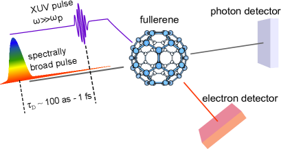
To be definite we concentrate here on the attosecond (as) evolution of the dielectric response in finite systems as monitored by the light absorption and refraction in fullerenes. The time-non-resolved (we call it hereafter steady-state) absorption of the fullerene Kroto et al. (1985); Orlandi and Negri (2002); Dresselhaus et al. (1996), in our case C60, can be accessed by analyzing the absorbed components from an impinging moderate intensity, broadband linear-polarized pulse. To monitor the attosecond buildup in absorption, we suggest that at a time $t=0$ an XUV attosecond pulse ionizes C60 and the change in the absorption at a time delay $\tau_{{}_{\rm D}}$ thereafter is recorded, as sketched in Fig. 1. For negative $\tau_{{}_{\rm D}}$ we obtain the absorption of C60 and for large (few femtoseconds) $\tau_{{}_{\rm D}}$ we expect the steady-state absorption of C${}_{60}^{+}$. Equilibration in the limit $t\rightarrow\infty$ proceeds via electronic, plasmonic and finally ionic channels, each having a distinct time scale; the ions are frozen at the as timescale. We focus on the plasma frequency ($\omega_{\rm p}$) regime where the absorption and refraction show strong modulations Bonin and Kresin (1997). The change of $\omega_{\rm p}$ for $t>0$ is evident from a qualitative consideration of the square root dependence on the density: The valence band of C60 accommodates 240 electrons (originating from the $2s$ and $2p$ states of each carbon atom) that form 180 $\sigma$-type and 60 $\pi$-type molecular orbitals Orlandi and Negri (2002). The highest occupied molecular orbital (HOMO) is five-fold degenerate. Its complete depletion by the XUV pulse reduces the number of particles by 4%, or red-shifts the collective response by 2%. As theoretically quantified below, even a single-photoionization event has a significant impact on the plasmon dynamics.

II Theoretical formulation

C60 has a size below 1 nm Dresselhaus et al. (1996), its electronic and optical properties for $t<0$ and $t\rightarrow\infty$ are well-documented Orlandi and Negri (2002); Dresselhaus et al. (1996). Also C60 is readily available, very stable, and has an ionization potential of $\approx$7.5 eV and an electron affinity of 2 eV. It also exists in a well-studied crystalline form (fullerite) Kratschmer et al. (1990). The collective response is marked by a giant plasmon resonance at $\approx 22$ eV Bertsch et al. (1991) that was investigated experimentally in the solid Hansen et al. (1991); Sohmen et al. (1992) and the gas phase Hertel et al. (1992). Considerable efforts were devoted to clarify quantitatively the experiments Bauernschmitt et al. (1998); Berkowitz (1999). It was not until recently however that the existence of a second plasmon peak at higher energy ($\approx 39$ eV) but with a lower oscillator strength was experimentally confirmed Reinköster et al. (2004); Scully et al. (2005). Theoretically, the presence of two collective modes follows from a classical dielectric shell model Mukhopadhyay and Lundqvist (1975); Lambin et al. (1992); Östling et al. (1993, 1996); Vasvari (1996). The quantitative description, as we are seeking here, is a challenging task, however. Quantum mechanical approaches utilize either the tight-binding (TB) model for the valence electrons Bertsch et al. (1991) or the jellium shell model Puska and Nieminen (1993); Yabana and Bertsch (1993); Ivanov et al. (2003); Scully et al. (2005); Madjet et al. (2008). The linear response to an external electric field is calculated either using the random phase approximation (RPA) for the polarization propagator ($\chi$) (in the case of the TB Bertsch et al. (1991) and some of the density-functional-based (DFT) models Yabana and Bertsch (1993); Ivanov et al. (2003)), or by implementing the time-dependent DFT (TDDFT) Puska and Nieminen (1993); Scully et al. (2005); Madjet et al. (2008). Until now TDDFT seems to deliver the best agreement with experiments, however, the theory describes correctly either the position of the high energy plasmon resonance or, with the help of an adjustable parameter, the position of the lower energy plasmon resonance Scully et al. (2005); Madjet et al. (2008).

Refer to caption
Figure 1: (Color online) A schematic of the considered setup. An attosecond XUV pulse ionizes a fullerene. After a time delay $\tau_{{}_{\rm D}}$ the time-dependent absorption of the sample is studied by analyzing the absorption of broadband, linear-polarized pulse.

Here we develop an approach that rests on three steps: 1. We utilize quantum chemical ab-initio techniques to capture accurately the stationary, single-particle electronic structure. 2. These states are expressed in a basis appropriate for many-body calculations which we perform within the linear response theory (i.e., the random phase approximation) to obtain the steady-state collective response. 3. With both quantities at hand we perform quantum kinetic calculations within the density matrix formalism to obtain the time and the frequency dependent polarizability $\alpha(E,t=\tau_{{}_{\rm D}})$. The imaginary and the real part of $\alpha(E,t)$ deliver then respectively the time-dependent absorption and refraction properties of the sample Bonin and Kresin (1997).

We showed recently Pavlyukh and Berakdar (2009, 2010, 2011) that the wave function $\Psi_{\epsilon}(\vec{r})$ of the valence band electrons with an energy $\epsilon=\varepsilon_{nl}$, as obtained from first principle calculations, is expressible to a good approximation as a product of a radial part $R_{n}(r)$ (having $n-1$ nodes) and an angular part described by spherical harmonics $Y_{lm}(\Omega)$ with $l,m$ being the orbital and magnetic quantum numbers ($\vec{r}\equiv(r,\Omega)$ identifies the electron position, cf. Ref. Sup ) Yabana and Bertsch (1993); Pavlyukh and Berakdar (2009). This procedure is shown Pavlyukh and Berakdar (2009) to be valid for C48N12, B80, C60, C240, C540, C20H20, and Au72. Thus, the theory presented below is readily applicable to these systems; for the sake of clarity the discussion is restricted to C60, however. For C60 the two occupied radial subbands $\varepsilon_{n=1\,l}$ and $\varepsilon_{n=2\,l}$ are separated by approximately $17.5~{}$eV. The HOMO-LUMO gap as determined by our ab-initio calculations ($E_{\rm g}\approx 5.5$ eV) as well as some structural information are encapsulated in the energy spectrum $\varepsilon_{nl}$ (cf. Sup ). These data allow us to perform the mapping of the unperturbed system to the single-particle Hamiltonian $\hat{H}_{0}$ with the states $\phi_{\alpha}\equiv\phi_{nlm}=R_{n}(r)Y_{lm}(\Omega)$ and the spectrum $\varepsilon_{nl}$. These single particle states are then taken as the basis to express the density operator $\hat{\rho}$. Our theoretical description of the charge dynamics is based on the resulting density matrix $\mathrm{\rho}$.

Refer to caption
Figure 2: (Color online) Energy dependence of the (a) real and (b) imaginary parts of the dipolar polarizability $\alpha(E)$ of C60 in the long-time limit. Insets to (a) show the calculated spatial densities of the plasmonic modes, corresponding to the peaks in the spectrum, in any plane crossing the center of the molecule and being parallel to the polarization of the external electric field. Dotted lines result from the approximation including only intraband collective excitations. Inset to (b) shows the difference in the spectra between C60 and C${}_{60}^{+}$ for the case of refraction.

We are interested in two types of external perturbations $\hat{V}^{\rm ext}$ that trigger the evolution: (i) a broad band, low-intensity light pulse probing the plasmonic response and (ii) a sudden change in the population upon a single ionization of C60 by the attosecond XUV pulse. Formally, the latter change is described by a time-dependent occupation function $f_{nl}(t)$. To simulate the plasmonic response, we employ the Heisenberg equation of motion for the density matrix $\hat{\rho}$, the mean-field approximation and the linear response to the external driving. The relaxation within a time $\tau$ due to collisions we treat within the particle-conserving relaxation time approximation Mermin (1970). This approach has been successfully tested for a variety of systems Morawetz et al. (2005); Huber et al. (2001); Borisov et al. (2004); García de Abajo (2010); Tanuma et al. (2011). It should be emphasized, however, that we are interested in the dynamics at times much shorter than $\tau$. The equation of motion for $\hat{\rho}$ reads as

$$\frac{\partial\hat{\rho}}{\partial t}+\frac{i}{\hbar}\left[\hat{H_{0}}+\hat{V}^{\rm ind}+\hat{V}^{\rm ext},\hat{\rho}\right]=\frac{\hat{\rho}^{\rm l.e.}-\hat{\rho}}{\tau}.$$ (1)

The induced potential $\hat{V}^{\rm ind}$ has to be determined self-consistently from the induced charge density as derived from the change in the density operator $\hat{\rho}$ [to find $\hat{\rho}$ we need $\hat{V}^{\rm ind}$ in Eq. (1)]. $\hat{\rho}^{\rm l.e.}$ is the local equilibrium density operator. The corresponding locally relaxed density $\rho^{\rm l.e.}(\vec{r},t)$ is the distribution that, at any given instant, would be in equilibrium in the presence of $\hat{V}^{\rm ext}$ and $\hat{V}^{\rm ind}$ while satisfying the charge conservation  Mermin (1970). Technically, we express $\hat{\rho}$ in the basis {$\phi_{\alpha}(\vec{r})$} and expand to first order around the equilibrium, i.e. $\rho_{\alpha\beta}(t)=\langle\alpha|\hat{\rho}(t)|\beta\rangle=f_{\alpha}(t)\delta_{\alpha\beta}+\delta\rho_{\alpha\beta}(t);\quad\rho^{\rm l.e.}_{\alpha\beta}(t)=\langle\alpha|\hat{\rho}^{\rm l.e.}(t)|\beta\rangle=f_{\alpha}(t)\delta_{\alpha\beta}+{\pi^{0}_{\alpha\beta}(t)}\delta\mu_{\alpha\beta}(t),$ where ${\pi^{0}_{\alpha\beta}(t)}=\frac{f_{\alpha}(t)-f_{\beta}(t)}{\varepsilon_{\alpha}-\varepsilon_{\beta}}$ and $\delta\mbox{\boldmath$\mathrm{\mu}$}(t)$ is the matrix corresponding to the local chemical potential (full details are given in Appendix A).

Application of an external linearly-polarized electric field with an amplitude ${\cal E}_{0}$, polarization direction $\vec{\rm e}$, and frequency $\omega$, that corresponds to $\hat{V}^{\rm ext}(t)=-e{\vec{r}\cdot\vec{\rm e}}{\cal E}_{0}e^{-i\omega t}$ ($e$ is the electron charge), leads to the change of the density matrix $\delta\mbox{\boldmath$\mathrm{\rho}$}(t)$ which in linear response is governed by the two-times response function $\mbox{\boldmath$\mathrm{\chi}$}(t,t^{\prime})$, i.e. ${\delta\mbox{\boldmath$\mathrm{\rho}$}(t)}=\int_{-\infty}^{t}\!\!{\rm d}t^{\prime}\;\mbox{\boldmath$\mathrm{\chi}$}(t,t^{\prime}){\mbox{\boldmath$\mathrm{V}$}^{\mathrm{ext}}(t^{\prime})}\>.$ The induced dipole moment derives from $\vec{P}(t)={\rm Tr}\left[e\vec{r}\delta\hat{\rho}(t)\right]$. For spherical molecules, reducing all quantities to their radial components, we find (see Appendix E)

$$P(t)=-\frac{4\pi}{3}e^{2}{\cal E}_{0}\int_{-\infty}^{t}\!\!{\rm d}t^{\prime}\;\mbox{\boldmath$\mathrm{r}$}^{T}\mbox{\boldmath$\mathrm{\chi}$}(t,t^{\prime})\mbox{\boldmath$\mathrm{r}$}e^{-i\omega t^{\prime}}{\>,}$$

where the elements of $\mathrm{r}$ are $r_{nn^{\prime}}=r_{n^{\prime}n}=\langle n|r|n^{\prime}\rangle$. Introducing the dimensionless, Fourier-transformed response function ($\tilde{\mbox{\boldmath$\mathrm{r}$}}={\mbox{\boldmath$\mathrm{r}$}}/r_{0}$, $r_{0}$ is the fullerene average radius and $\epsilon_{0}$ is the vacuum permittivity)

$$\mbox{\boldmath$\mathrm{z}$}(\omega,t)=\frac{e^{2}}{3\epsilon_{0}r_{0}}\int_{0}^{\infty}\!\!{\rm d}\tau\;e^{i\omega\tau}\mbox{\boldmath$\mathrm{\chi}$}(t,t-\tau)\tilde{\mbox{\boldmath$\mathrm{r}$}}\;,$$ (2)

we find $P(\omega;t)=-4\pi r_{0}^{3}\epsilon_{0}{\cal E}_{0}{\rm e}^{-i\omega t}\tilde{\mbox{\boldmath$\mathrm{r}$}}^{T}\mbox{\boldmath$\mathrm{z}$}(\omega,t)\;$. The time and frequency-dependent dipolar polarizability is then calculated numerically as

$$\alpha(\omega,t)=-r_{0}^{3}\tilde{\mbox{\boldmath$\mathrm{r}$}}^{T}\mbox{\boldmath$\mathrm{z}$}(\omega,t)\;.$$ (3)

(in SI units, $\alpha_{\rm SI}=4\pi\epsilon_{0}\alpha$). The explicit equation for the evolution of $\mbox{\boldmath$\mathrm{z}$}(\omega,t)$, and therefore of $\alpha(\omega,t)$, following from Eq. (1) we included in Appendix A.

For an insight into the numerical results we construct an analytical model based on the following: For C60 (and generally for ,,spherical” molecules) we find that the intraband components $z_{11}(\omega,t)$ and $z_{22}(\omega,t)$ of the response function are hardly influenced by the interband components $z_{12}(\omega,t)$ and $z_{21}(\omega,t)$ (details are in Appendix D). In this approximation, considering only the intraband terms we infer a system of two coupled equations for $z_{11}(\omega,t)$ and $z_{22}(\omega,t)$

$$\begin{split}\Big{[}\partial^{2}_{t}+&\left(\frac{1}{\tau}-\!2i\omega\right)\partial_{t}+\omega_{{\rm F},n}^{2}\!-\!\omega^{2}\!-\!i\frac{\omega}{\tau}\Big{]}z_{nn}(\omega,t)\\ +&\omega_{{\rm p},n}^{2}\sum_{n^{\prime}=1,2}\tilde{g}_{nn,n^{\prime}n^{\prime}}z_{n^{\prime}n^{\prime}}(\omega,t)=-\omega_{{\rm p},n}^{2}\;,\\ \end{split}$$ (4)

where the stationary matrix $\tilde{\mbox{\boldmath$\mathrm{g}$}}$ is explicitly defined in Appendix B and $\omega_{{\rm p},n}^{2}=1/\hbar^{2}\times e^{2}\sqrt{2N_{n}}/(6\pi\epsilon_{0}r_{0})\times\hbar\omega_{{\rm F},n}$. Here $N_{n}$ is the number of electrons in the $n$-th radial subband. For C60 in the equilibrium we have $N_{1}=180$ and $N_{2}=60$. $\hbar\omega_{{\rm F},n}$ are the energy distances between the highest occupied state in the $n$-th radial subband and the unoccupied state in the same subband having the value of $l$ that is greater by one. On the same approximation level Eq. (3) simplifies to $\alpha(\omega,t)=-r_{0}^{3}\left[z_{11}(\omega,t)+z_{22}(\omega,t)\right]$ meaning that the interband components can be then neglected when calculating $\alpha(\omega,t)$. In such a consideration the dynamics of the electron density in two different radial channels are still coupled via the induced fields like in concentric nanoshells Radloff and Halas (2004).

III Steady-state collective response

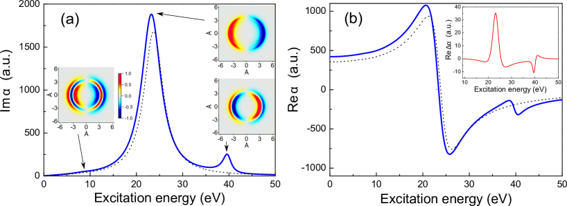
Absorption and refraction spectra of the C60 and C${}_{60}^{+}$ in the long-time limit (i.e. $\tau_{{}_{\rm D}}<0$) are shown in Fig. 2. The responses of C${}_{60}^{+}$ and C60 are quite similar [cf. inset in Fig. 2(b)] which is in agreement with the existing theory and experiment Scully et al. (2005); Madjet et al. (2008). Our C60 calculations exhibit two peaks at 23.2 eV and at 39.6 eV in the absorption spectrum which correspond to plasmon excitations and agree very well with experiment Scully et al. (2005). The width of the measured main plasmon resonance is reported to be $\approx 5$ eV which sets the scale for the relaxation time $\tau$. With $\sigma(E)=\frac{4\pi E}{\hbar c}{\rm Im}\alpha(E)$ Bonin and Kresin (1997), where $c$ is the speed of light, we find the corresponding absorption cross-sections $\sigma(E)$ to be $4.1\times 10^{3}$ Mb for the main peak and $9.4\times 10^{2}$ Mb for the higher energy peak. This yields relative heights of the peaks that are in qualitative agreement with the experiments and with the time-dependent DFT results Puska and Nieminen (1993); Madjet et al. (2008). There is also a weak low energy contribution at $\approx$ 9 eV. Such structures in the absorption have been attributed to single-electron transitions Bauernschmitt et al. (1998); Orlandi and Negri (2002). Our calculated resonance has a collective character and is energetically in the proximity of the single-electron excitations making it difficult for an observation via absorption. As well-established Bonin and Kresin (1997), the peaks in the absorption (refraction) are symmetric (antisymmetric) with respect to reflection at the respective central frequency.

Refer to caption
Figure 3: (Color online) (a) Difference between the imaginary part of the dipolar polarizability ${\rm Im}\alpha(E,t)$ after removing one electron from the highest occupied state of C60 in the second (upper) branch at $t=0$ and its long-time limit for C${}_{60}^{+}$, i.e. ${\rm Im}\alpha_{{\rm C}_{60}^{+}}(E)$. (b) The same dependence for the real part change of $\alpha(E,t)$. (c) Time dependence of the imaginary part of the dipolar polarizability $\mbox{Im}\hskip 2.0pt\alpha(E,t)$ of the excited fullerene molecule at fixed energy values, $E=24.6~{}$eV and $E=38.8~{}$eV, taken close to the main and higher energy resonance positions of the stationary response, respectively. Time intervals $T=\pi\hbar/E$ indicated by the horizontal double-arrow lines are close to the observed oscillation periods for each of the dependencies: $T=84$ as and $T=53$ as , respectively.

The approximation including only intraband collective excitations, i.e. considering the stationary solution of Eq. (4), gives a very good description of the main peak in the spectrum (see Fig. 2), but misses the higher energy plasmon. The last is caused by interband collective excitations (i.e. governed by $z_{12}$ and $z_{21}$) that are still influenced strongly by the intraband response. The interband excitations shift slightly the main plasmon resonance to lower energies and enhance its strength. The $f$-sum rule Apell et al. (1996); Ivanov et al. (2003); Pal et al. (2011) for the absorption is fulfilled only approximately, particularly because higher energy states in the continuum and close to it are not included in our model. However, these states contribute mostly to the background of the spectrum. For a further insight we show the calculated spatial distributions of the induced charge densities at the maximal absorption [insets in Fig. 2(a)]. The oscillation amplitude depends linearly on the external field strength. The interband character of the the higher energy plasmon excitation is evident. Its radial structure is determined by the product $R_{1}(r)R_{2}(r)$ and has therefore one node located in the middle of the fullerene cage. The angular dependence of the modes in and out of the depicted plane is governed by their dipolar character. The radial structure of the density oscillation at the main plasmon peak shows a constructive superposition of the radial electronic radial density of the first $|R_{1}(r)|^{2}$ and the second $|R_{2}(r)|^{2}$ radial channels that oscillate in phase. In contrast, we observe an out-of-phase oscillation of the densities in different channels at 9 eV. Both cases are collective intraband electronic excitations.

IV Transient dynamics

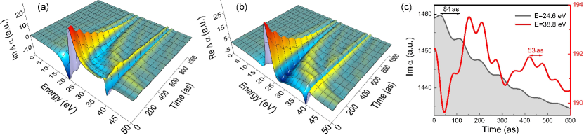
Having assessed successfully the steady-state response we move on to the attosecond transient dynamics. We focus on the setup shown in Fig. 1. At $t=0$ the XUV pulse with energy $\omega\gg\omega_{\rm p}$ and a duration $<100$ as changes the population swiftly in C60 by ejecting one electron. To access the transient absorption or refraction let us assume the photoelectron is emitted at $t=0$ from the second radial band leaving C${}_{60}^{+}$ (we find similar results for multiple XUV ionization). For all time moments before the ionization the time-dependent response $\alpha(E,t<0)$ is equal to its steady-state value $\alpha_{{\rm C}_{60}}(E)$ for C60. At $t>0$ we solve for the dynamics of $\alpha(E,t)$, which for long times approaches the steady-state value $\alpha_{{\rm C}_{60}^{+}}(E)$ for C${}_{60}^{+}$. The results in Figs. 3(a) and 3(b) illustrate the change in the imaginary (absorption) and real (refraction) parts of the polarizability by evaluating $\Delta\alpha(E,t)=\alpha_{{\rm C}_{60}}(E,t)-\alpha_{{\rm C}_{60}^{+}}(E)$. The transient dynamics shows a rich structure evolving over approximately 2 fs. For $1$ fs the remainder of the vanishing difference between $\alpha(E,t)$ and $\alpha_{{\rm C}_{60}^{+}}(E)$ is still visible in Figs. 3(a) and 3(b). For $t<100$ as the response is basically determined by that of C60, i.e. it takes around 100 as for C${}_{60}^{+}$ to start responding collectively and it attains its full, steady state response for $t>1$ fs. The reason of this inertia is the finite mass of the carriers. Three marked general transient features can be distilled from Fig. 3. The dispersive hump starting around 200 as is due to the sudden change in the population (and hence the wide frequency perturbation) brought about by the shortness of the XUV pulse. Furthermore, in addition to the relaxation to the steady-state response we observe an oscillatory behavior in time with a certain frequency. This behavior is most obvious around $\omega_{\rm p}$ (cf. Fig. 3). The origin of these oscillations is comprehensible from a consideration of the response of the fullerene molecule in the lowest approximation: As we demonstrated by Eq. (4) the response resembles two coupled damped harmonic oscillators. For photon frequencies $\omega$ close to the main peak position the model can even be further simplified and the spectra are determined approximately by the dynamics of a single driven damped harmonic oscillator with the frequency corresponding to the main peak position. Hence, the feature in the response we can now understand from the known properties of the driven, damped harmonic motion. On a short time scale this dynamics is governed by a combined decay and oscillations with a frequency around $2\omega$, which is clearly observed in the full-fledge calculations shown in Fig. 3(c) for $\mbox{Im}\hskip 2.0pt\alpha(E,t)$ at $E=24.6~{}$eV (time period corresponding to $2\omega$ is indicated by a horizontal double-arrow line for comparison). The dynamics of $\mbox{Im}\hskip 2.0pt\alpha(E,t)$ for fixed energy $E=38.8~{}$eV in the vicinity of the higher energy peak is contributed to by more frequencies because the higher energy plasmon is strongly influenced by the main plasmon. However, oscillations corresponding to $2\omega$ are also seen.

V Summary

We developed a framework for the attosecond collective response in finite systems with spherical symmetry and applied it to fullerenes. The predicted marked features in the transient absorption and refraction should be accessible with current attosecond metrology. The discovered attosecond dynamics in the optical response points to new opportunities for optoelectronic devices at the sub-femtosecond time scale.

Acknowledgements

It is a pleasure to acknowledge clarifying discussions on the experiments with E. Goulielmakis and R. Ernstorfer.

Appendix A Derivation of the linear response equations

The transient time and energy-dependent polarizability $\alpha(t,E)$ is governed, to a first order (linear response), by the two-time response function $\chi(t,t^{\prime})$. For the determination of $\chi(t,t^{\prime})$ we setup a calculational scheme based on the solution of the Heisenberg equation of motion for the density matrix $\hat{\rho}$ under the influence of the external field $\hat{V}^{\rm ext}$ in the mean-field approximation that leads to Eq. (1). In the basis $\{\phi_{\alpha}\}$ we find the density matrix elements as $\rho_{nlm,n^{\prime}l^{\prime}m^{\prime}}=\langle nlm|\hat{\rho}|n^{\prime}l^{\prime}m^{\prime}\rangle$. From the change in the density matrix $\delta\rho_{nlm,n^{\prime}l^{\prime}m^{\prime}}$ we calculate the change in the charge density

$$\delta n(\vec{r})=\sum_{lm}\delta n_{lm}(r)Y_{lm}(\theta,\phi)\;,$$ (5)

where

$$\delta n_{lm}(r)=\sum_{n^{\prime}n^{\prime\prime}}s_{n^{\prime}n^{\prime\prime}}(r)\delta n^{n^{\prime}n^{\prime\prime}}_{lm}\;,$$ (6)
$$s_{n^{\prime}n^{\prime\prime}}(r)=R_{n^{\prime}}(r)R_{n^{\prime\prime}}(r)\;,$$ (7)
$$\delta n^{n^{\prime}n^{\prime\prime}}_{lm}=\sum_{l^{\prime}m^{\prime},l^{\prime\prime}m^{\prime\prime}}y^{l^{\prime}m^{\prime}}_{lm,l^{\prime\prime}m^{\prime\prime}}\delta\rho_{nlm,n^{\prime}l^{\prime}m^{\prime}}\;,$$ (8)
$$\begin{split}y^{lm}_{l^{\prime}m^{\prime},l^{\prime\prime}m^{\prime\prime}}&=\int\!\!{\rm d}\Omega\;Y_{lm}^{*}(\Omega)Y_{l^{\prime}m^{\prime}}(\Omega)Y_{l^{\prime}m^{\prime}}(\Omega)\\ &=\sqrt{\frac{(2l^{\prime}+1)(2l^{\prime\prime}+1)}{4\pi(2l+1)}}\;C^{l0}_{l^{\prime}0,l^{\prime\prime}0}C^{lm}_{l^{\prime}m^{\prime},l^{\prime\prime}m^{\prime\prime}}\;.\end{split}$$ (9)

$C^{lm}_{l^{\prime}m^{\prime},l^{\prime\prime}m^{\prime\prime}}$ are Clebsch-Gordan coefficients. The change in the charge density determines the induced potential $\hat{V}^{\rm ind}$ leading thus to a self-consistent procedure.

In the basis $\{\phi_{\alpha}\}$ the Heisenberg equation of motion for the density matrix (1) reads:

$$\begin{split}\frac{\partial\rho_{nlm,n^{\prime}l^{\prime}m^{\prime}}}{\partial t}=&-\frac{1}{\hbar}\left[i(\varepsilon_{nlm}-\varepsilon_{n^{\prime}l^{\prime}m^{\prime}})+\frac{\hbar}{\tau}\right]\rho_{nlm,n^{\prime}l^{\prime}m^{\prime}}\\ &-\frac{i}{\hbar}\sum_{n^{\prime\prime}l^{\prime\prime}m^{\prime\prime}}\left(\rho_{n^{\prime\prime}l^{\prime\prime}m^{\prime\prime},n^{\prime}l^{\prime}m^{\prime}}V_{nlm,n^{\prime\prime}l^{\prime\prime}m^{\prime\prime}}\right.\\ &\hskip 51.21504pt\left.-\rho_{nlm,n^{\prime\prime}l^{\prime\prime}m^{\prime\prime}}V_{n^{\prime\prime}l^{\prime\prime}m^{\prime\prime},n^{\prime}l^{\prime}m^{\prime}}\right)\\ &+\frac{\rho_{nlm,n^{\prime}l^{\prime}m^{\prime}}^{\rm l.e.}-\rho_{nlm,n^{\prime}l^{\prime}m^{\prime}}}{\tau}\;.\end{split}$$ (10)

Here $\varepsilon_{nlm}$ are the single particle energies (cf. Ref. Sup ). The matrix elements of the Coulomb potential are cast as

$$\begin{split}V_{nlm,n^{\prime}l^{\prime}m^{\prime}}&=\langle nlm|\hat{V}^{\rm ind}+\hat{V}^{\rm ext}|n^{\prime}l^{\prime}m^{\prime}\rangle\\ &=V^{\rm ind}_{nlm,n^{\prime}l^{\prime}m^{\prime}}+V^{\rm ext}_{nlm,n^{\prime}l^{\prime}m^{\prime}}\;,\end{split}$$ (11)

where

$$V^{\rm ext}_{nlm,n^{\prime}l^{\prime}m^{\prime}}=\sum_{l^{\prime\prime}m^{\prime\prime}}y^{lm}_{l^{\prime}m^{\prime},l^{\prime\prime}m^{\prime\prime}}V^{{\rm ext},nn^{\prime}}_{l^{\prime\prime}m^{\prime\prime}}\;$$ (12)

and

$$V^{{\rm ext},nn^{\prime}}_{l^{\prime\prime}m^{\prime\prime}}=\int\!\!r^{2}{\rm d}rs_{nn^{\prime}}(r)V_{l^{\prime\prime}m^{\prime\prime}}^{\rm ext}(r)\;.$$ (13)

Upon solving the Poisson equation (see Appendix B) we find for the matrix elements of the potential $V^{\rm ind}(\vec{r})=e\Phi(\vec{r})$ induced by the change in the charge density $\delta n(\vec{r})$ the following expression

$$V^{\rm ind}_{nlm,n^{\prime}l^{\prime}m^{\prime}}=\frac{e^{2}}{\epsilon_{0}}\sum_{n_{1}n_{2}}\sum_{l^{\prime\prime}m^{\prime\prime}}y^{lm}_{l^{\prime}m^{\prime},l^{\prime\prime}m^{\prime\prime}}g^{l^{\prime\prime}}_{nn^{\prime},n_{1}n_{2}}\delta n^{n_{1},n_{2}}_{l^{\prime\prime}m^{\prime\prime}}\;.$$ (14)

The coefficients $g^{l^{\prime\prime}}_{nn^{\prime},n_{1}n_{2}}$ are defined in Appendix B by Eq. (47).

We are interested in the linear response and expand therefore the density matrix around the equilibrium distribution $f_{nlm}^{0}$ as

$$\rho_{nlm,n^{\prime}l^{\prime}m^{\prime}}=f_{nlm}^{0}+\delta\rho_{nlm,n^{\prime}l^{\prime}m^{\prime}}\;.$$ (15)

Thus, $\delta\rho_{nlm,n^{\prime}l^{\prime}m^{\prime}}$ is a small perturbation. The elements of the local equilibrium density matrix including the lowest order correction with respect to the equilibrium density matrix are given then by Mermin (1970)

$$\begin{split}\rho_{nlm,n^{\prime}l^{\prime}m^{\prime}}^{\rm l.e.}=&f_{nlm}^{0}\delta_{nn^{\prime}}\delta_{ll^{\prime}}\delta_{mm^{\prime}}\\ &-\frac{f_{nlm}^{0}-f_{n^{\prime}l^{\prime}m^{\prime}}^{0}}{\varepsilon_{nlm}-\varepsilon_{n^{\prime}l^{\prime}m^{\prime}}}\delta\mu_{nlm,n^{\prime}l^{\prime}m^{\prime}}\;.\end{split}$$ (16)

Here the components of the chemical potential can be expressed as

$$\delta\mu_{n^{\prime}l^{\prime}m^{\prime},n^{\prime\prime}l^{\prime\prime}m^{\prime\prime}}=\sum_{\tilde{l}\tilde{m}}y^{l^{\prime}m^{\prime}}_{l^{\prime\prime}m^{\prime\prime},\tilde{l}\tilde{m}}\delta\mu^{n^{\prime}n^{\prime\prime}}_{\tilde{l}\tilde{m}}\;.$$ (17)

We require density conservation, meaning that $n^{n^{\prime}n^{\prime\prime}}_{lm}=n^{{\rm l.e.},n^{\prime}n^{\prime\prime}}_{lm}$ which in turn leads to

$$\delta n^{n^{\prime}n^{\prime\prime}}_{lm}=\sum_{\tilde{l}\tilde{m}}M^{n^{\prime}n^{\prime\prime}}_{lm,\tilde{l}\tilde{m}}\delta\mu^{n^{\prime}n^{\prime\prime}}_{\tilde{l}\tilde{m}}\;,$$ (18)

where

$$M^{n^{\prime}n^{\prime\prime}}_{lm,\tilde{l}\tilde{m}}=-\!\!\!\!\sum_{l^{\prime}m^{\prime},l^{\prime\prime}m^{\prime\prime}}y^{l^{\prime}m^{\prime}}_{lm,l^{\prime\prime}m^{\prime\prime}}y^{l^{\prime}m^{\prime}}_{l^{\prime\prime}m^{\prime\prime},\tilde{l}\tilde{m}}\frac{f^{0}_{n^{\prime}l^{\prime}m^{\prime}}-f^{0}_{n^{\prime\prime}l^{\prime\prime}m^{\prime\prime}}}{\varepsilon_{n^{\prime}l^{\prime}m^{\prime}}-\varepsilon_{n^{\prime\prime}l^{\prime\prime}m^{\prime\prime}}}\;.$$ (19)

In general, $\delta\mu^{n^{\prime}n^{\prime\prime}}_{\tilde{l}\tilde{m}}$ is determined from Eq. (18) by solving a system of linear equations for each pair of indexes $n^{\prime},n^{\prime\prime}$. This step of the calculation is significantly simplified by neglecting the energy splitting of the multiplet with the same $l$, i.e. by writing $\varepsilon_{nlm}=\varepsilon_{nlm^{\prime}}\equiv\varepsilon_{nl}$ and therefore $f^{0}_{nlm}=f^{0}_{nlm^{\prime}}\equiv f^{0}_{nl}$, which is a good approximation for “spherical” molecules such as C60, as confirmed by the ab-initio calculations. Adopting this approximation we conclude that (cf. Appendix C)

$$\delta\mu^{n^{\prime}n^{\prime\prime}}_{lm}=\frac{1}{M^{n^{\prime}n^{\prime\prime}}_{l}}\delta n^{n^{\prime}n^{\prime\prime}}_{lm}\;,$$ (20)

where

$$M^{n^{\prime}n^{\prime\prime}}_{l}=-\sum_{l^{\prime}l^{\prime\prime}}K^{l}_{l^{\prime}l^{\prime\prime}}\frac{f^{0}_{n^{\prime}l^{\prime}}-f^{0}_{n^{\prime\prime}l^{\prime\prime}}}{\varepsilon_{n^{\prime}l^{\prime}}-\varepsilon_{n^{\prime\prime}l^{\prime\prime}}}\;$$ (21)

and

$$K^{l}_{l^{\prime}l^{\prime\prime}}=\frac{(2l^{\prime}+1)(2l^{\prime\prime}+1)}{4\pi(2l+1)}\left[C^{l0}_{l^{\prime}0,l^{\prime\prime}0}\right]^{2}\;.$$ (22)

Gathering the informations in Eq. (17) and Eq. (20) we can state

$$\delta\mu_{n^{\prime}l^{\prime}m^{\prime},n^{\prime\prime}l^{\prime\prime}m^{\prime\prime}}=\sum_{\tilde{l}\tilde{m}}y^{l^{\prime}m^{\prime}}_{l^{\prime\prime}m^{\prime\prime},\tilde{l}\tilde{m}}\frac{1}{M^{n^{\prime}n^{\prime\prime}}_{\tilde{l}}}\delta n^{n^{\prime}n^{\prime\prime}}_{\tilde{l}\tilde{m}}\;.$$ (23)

From Eq. (10) we deduce then the following determining equation for the change in the density matrix

$$\begin{split}\frac{\partial\delta\rho_{nlm,n^{\prime}l^{\prime}m^{\prime}}}{\partial t}=&-\frac{1}{\hbar}\left[i(\varepsilon_{nl}-\varepsilon_{n^{\prime}l^{\prime}})+\frac{\hbar}{\tau}\right]\delta\rho_{nlm,n^{\prime}l^{\prime}m^{\prime}}\\ &+\frac{i}{\hbar}(f^{0}_{nl}-f^{0}_{n^{\prime}l^{\prime}})V_{nlm,n^{\prime}l^{\prime}m^{\prime}}-\frac{1}{\tau}\frac{f^{0}_{nl}-f^{0}_{n^{\prime}l^{\prime}}}{\varepsilon_{nl}-\varepsilon_{n^{\prime}l^{\prime}}}\delta\mu_{nlm,n^{\prime}l^{\prime}m^{\prime}}\;.\end{split}$$ (24)

The solution of this equation is found as

$$\begin{split}\delta\rho_{nlm,n^{\prime}l^{\prime}m^{\prime}}(t)=\frac{i}{\hbar}\int_{-\infty}^{t}\!\!{\rm d}t^{\prime}e^{\left[\frac{i}{\hbar}(\varepsilon_{nl}-\varepsilon_{n^{\prime}l^{\prime}})+\frac{1}{\tau}\right](t-t^{\prime})}\bigg{\{}&\left[f^{0}_{nl}(t^{\prime})-f^{0}_{n^{\prime}l^{\prime}}(t^{\prime})\right]V_{nlm,n^{\prime}l^{\prime}m^{\prime}}(t^{\prime})\\ &+i\frac{\hbar}{\tau}\frac{f^{0}_{nl}(t^{\prime})-f^{0}_{n^{\prime}l^{\prime}}(t^{\prime})}{\varepsilon_{nl}-\varepsilon_{n^{\prime}l^{\prime}}}\delta\mu_{nlm,n^{\prime}l^{\prime}m^{\prime}}(t^{\prime})\bigg{\}}\;.\end{split}$$ (25)

Inserting Eqs. (14),(12) and (23) into Eq. (25) and summing the left and right hand sides weighted by $y^{l^{\prime}m^{\prime}}_{lm,l^{\prime\prime}m^{\prime\prime}}$ as in Eq. (8) we infer that

$$\begin{split}\delta n^{n^{\prime}n^{\prime\prime}}_{lm}=&\int_{-\infty}^{t}\!\!{\rm d}t^{\prime}\;\Pi^{n^{\prime}n^{\prime\prime}}_{l}(t,t^{\prime})V^{{\rm ext},n^{\prime}n^{\prime\prime}}_{lm}(t^{\prime})+\int_{-\infty}^{t}\!\!{\rm d}t^{\prime}\;\Pi^{n^{\prime}n^{\prime\prime}}_{l}(t,t^{\prime})\frac{e^{2}}{\epsilon_{0}}\sum_{n_{1}n_{2}}g^{l}_{n^{\prime}n^{\prime\prime},n_{1}n_{2}}\delta n^{n_{1}n_{2}}_{lm}(t^{\prime})\\ &+\int_{-\infty}^{t}\!\!{\rm d}t^{\prime}\;I^{n^{\prime}n^{\prime\prime}}_{l}(t,t^{\prime})\delta n^{n^{\prime}n^{\prime\prime}}_{lm}(t^{\prime})\;,\end{split}$$ (26)

where

$$\Pi^{n^{\prime}n^{\prime\prime}}_{l}(t,t^{\prime})=\frac{i}{\hbar}\sum_{l^{\prime}l^{\prime\prime}}K^{l}_{l^{\prime}l^{\prime\prime}}e^{\left[\frac{i}{\hbar}(\varepsilon_{n^{\prime}l^{\prime}}-\varepsilon_{n^{\prime\prime}l^{\prime\prime}})+\frac{1}{\tau}\right](t^{\prime}-t)}\left[f^{0}_{n^{\prime}l^{\prime}}(t^{\prime})-f^{0}_{n^{\prime\prime}l^{\prime\prime}}(t^{\prime})\right]\;,$$ (27)
$$I^{n^{\prime}n^{\prime\prime}}_{l}(t,t^{\prime})=-\frac{1}{\tau M_{l}^{n^{\prime}n^{\prime\prime}}}\sum_{l^{\prime}l^{\prime\prime}}K^{l}_{l^{\prime}l^{\prime\prime}}e^{\left[\frac{i}{\hbar}(\varepsilon_{n^{\prime}l^{\prime}}-\varepsilon_{n^{\prime\prime}l^{\prime\prime}})+\frac{1}{\tau}\right](t^{\prime}-t)}\frac{f^{0}_{n^{\prime}l^{\prime}}(t^{\prime})-f^{0}_{n^{\prime\prime}l^{\prime\prime}}(t^{\prime})}{\varepsilon_{n^{\prime}l^{\prime}}-\varepsilon_{n^{\prime\prime}l^{\prime\prime}}}\;.$$ (28)

This is the central integral equation, which has to be solved to arrive at the time-dependent density change induced by a perturbing external electric field.

We introduce the response function $\chi^{l}_{nn^{\prime},n_{1}n_{2}}(t,t^{\prime})$ as

$$\delta n^{n^{\prime}n^{\prime\prime}}_{lm}(t)=\int_{-\infty}^{t}\!\!{\rm d}t^{\prime}\;\sum_{n_{1}n_{2}}\chi^{l}_{n^{\prime}n^{\prime\prime},n_{1}n_{2}}(t,t^{\prime})V_{lm}^{{\rm ext},n_{1}n_{2}}(t^{\prime})\;.$$ (29)

Here we consider the perturbation by the external electric field in the dipole approximation. Therefore the calculation can be limited to the case $l=0$. In order to simplify notations, in the following we omit the corresponding index by all variables and coefficients.

Inserting the definition (29) into Eq. (26), changing the order of integration in the second term on the right hand side, comparing again with Eq. (29) and making use of the dipole approximation, we get the following integral equation for the response function:

$$\begin{split}\sum_{n_{1}n_{2}}\chi_{n^{\prime}n^{\prime\prime},n_{1}n_{2}}(t,t^{\prime})\tilde{r}_{n_{1}n_{2}}=&\Pi^{n^{\prime}n^{\prime\prime}}(t,t^{\prime})\tilde{r}_{n^{\prime}n^{\prime\prime}}\\ &+\int_{t^{\prime}}^{t}\!\!{\rm d}t^{\prime\prime}\;\frac{e^{2}}{\epsilon_{0}}\Pi^{n^{\prime}n^{\prime\prime}}(t,t^{\prime\prime})\sum_{n_{1}n_{2},n_{3}n_{4}}g_{n^{\prime}n^{\prime\prime},n_{1}n_{2}}\chi_{n_{1}n_{2},n_{3}n_{4}}(t^{\prime\prime},t^{\prime})\tilde{r}_{n_{3}n_{4}}\\ &+\int_{t^{\prime}}^{t}\!\!{\rm d}t^{\prime\prime}\;I^{n^{\prime}n^{\prime\prime}}(t,t^{\prime\prime})\sum_{n_{1}n_{2}}\chi_{n^{\prime}n^{\prime\prime},n_{1}n_{2}}(t^{\prime\prime},t^{\prime})\tilde{r}_{n_{1}n_{2}}\;,\end{split}$$ (30)

where the matrix elements $\tilde{r}_{nn^{\prime}}$ are given by $\tilde{r}_{n^{\prime}n^{\prime\prime}}=\frac{1}{r_{0}}\int\!\!r^{2}{\rm d}r\>s_{n^{\prime}n^{\prime\prime}}(r)r\;$ and are calculated by us using the radial functions for C60 from our ab-initio calculations. Here we have also taken into account that in the dipole approximation the identity $V^{{\rm ext},n_{1}n_{2}}\tilde{r}_{n^{\prime}n^{\prime\prime}}=V^{{\rm ext},n^{\prime}n^{\prime\prime}}\tilde{r}_{n_{1}n_{2}}$ holds. The corresponding time- and frequency-dependent response function is determined then by

$$z_{n^{\prime}n^{\prime\prime}}(\omega,t)=\frac{e^{2}g}{\epsilon_{0}}\int_{0}^{\infty}\!\!{\rm d}T\;e^{i\omega T}\sum_{n_{1},n_{2}}\chi_{n^{\prime}n^{\prime\prime},n_{1}n_{2}}(t,t-T)\tilde{r}_{n_{1}n_{2}}\;,$$ (31)

where $g=1/(3r_{0})$ and $\epsilon_{0}$ is the vacuum permittivity. Here $r_{0}\approx 6.745a_{{}_{\rm B}}$ is the average radius of the C60 atomic cage, where $a_{{}_{\rm B}}$ is the Bohr radius. After inserting Eq. (30) into Eq. (31) we arrive at the following system of integral equations for each frequency value $\omega$:

$$\begin{split}z_{n^{\prime}n^{\prime\prime}}\!(\omega,t)=&\int_{-\infty}^{t}\!\!{\rm d}t^{\prime}e^{i\omega(t-t^{\prime})}\tilde{r}_{n^{\prime}n^{\prime\prime}}W^{n^{\prime}n^{\prime\prime}}(t,t^{\prime})\\ &+\int_{-\infty}^{t}\!\!{\rm d}t^{\prime}e^{i\omega(t-t^{\prime})}W^{n^{\prime}n^{\prime\prime}}(t,t^{\prime})\sum_{n_{1},n_{2}}\tilde{g}_{n^{\prime}n^{\prime\prime},n_{1}n_{2}}z_{n_{1}n_{2}}(\omega,t^{\prime})\\ &+\int_{-\infty}^{t}\!\!{\rm d}t^{\prime}e^{i\omega(t-t^{\prime})}I^{n^{\prime}n^{\prime\prime}}(t,t^{\prime})z_{n^{\prime}n^{\prime\prime}}\!(\omega,t^{\prime})\;,\hskip 11.38092ptn^{\prime},n^{\prime\prime}=1,2\;;\end{split}$$ (32)

where $\tilde{g}_{n^{\prime}n^{\prime\prime},n_{1}n_{2}}=g_{n^{\prime}n^{\prime\prime},n_{1}n_{2}}/g$ and

$$W^{n^{\prime}n^{\prime\prime}}(t,t^{\prime})=\frac{e^{2}g}{\epsilon_{0}}\Pi^{n^{\prime}n^{\prime\prime}}(t,t^{\prime})\;.$$ (33)

Here $\Pi^{n^{\prime}n^{\prime\prime}}$ and $I^{n^{\prime}n^{\prime\prime}}(t,t^{\prime})$ are given by Eq. (27) and Eq. (28), respectively, with $l=1$. The system of equations (32) is solved numerically.

It can be shown (see section E) that the time- and frequency-dependent dipolar polarizability can be written as

$$\alpha(\omega,t)=-r_{0}^{3}\sum_{n^{\prime}n^{\prime\prime}}\tilde{r}_{n^{\prime}n^{\prime\prime}}z_{n^{\prime}n^{\prime\prime}}(\omega,t)\;.$$ (34)

Appendix B Calculation of the induced potential and its matrix elements

Here we determine the electrostatic potential $\Phi(\vec{r})$ induced by the change of the density in the spherical layer $n(\vec{r})$. The Poisson equation

$$\Delta\Phi(\vec{r})=-\frac{e}{\epsilon_{0}}n(\vec{r})$$ (35)

has then to be solved (SI units are used in this work). Its solution can be written using the Green’s function $G(\vec{r},\vec{r}^{\prime})$

$$\Phi(\vec{r})=-\frac{e}{\epsilon_{0}}\int G(\vec{r},\vec{r}^{\prime})n(\vec{r}^{\prime}){\rm d}^{3}\vec{r}^{\prime},$$ (36)

where

$$G(\vec{r},\vec{r}^{\prime})=-\frac{1}{4\pi\left|\vec{r}-\vec{r}^{\prime}\right|}\;.$$ (37)

Using the spherical geometry of the problem we apply the following decomposition for the Green’s function:

$$\frac{1}{\left|\vec{r}-\vec{r}^{\prime}\right|}=\sum_{l=0}^{\infty}\sum_{m=-l}^{l}\frac{4\pi}{2l+1}\frac{r_{<}^{l}}{r_{>}^{l+1}}Y_{lm}(\theta,\phi)Y^{*}_{lm}(\theta^{\prime},\phi^{\prime})\;,$$ (38)

where $r_{>}={\rm max}\{r,r^{\prime}\}$ and $r_{<}={\rm min}\{r,r^{\prime}\}$. Then we get the following expression for the potential

$$\begin{split}\Phi(\vec{r})=\frac{e}{\epsilon_{0}}\int{\rm d}^{3}\vec{r}^{\prime}\sum_{l=0}^{\infty}\sum_{m=-l}^{l}&\frac{1}{2l+1}\frac{r_{<}^{l}}{r_{>}^{l+1}}Y_{lm}(\theta,\phi)\\ &\times Y^{*}_{lm}(\theta^{\prime},\phi^{\prime})n(\vec{r}^{\prime})\;.\end{split}$$ (39)

To proceed further we decompose $n(\vec{r}^{\prime})$ in spherical harmonics

$$n(r,\theta,\phi)=\sum_{lm}n_{lm}(r)Y_{lm}(\theta,\phi),$$ (40)

where the radial-dependent angular components of the density can be found as

$$n_{lm}(r)=\sum_{n^{\prime}n^{\prime\prime}}s_{n^{\prime}n^{\prime\prime}}(r)n^{n^{\prime}n^{\prime\prime}}_{lm}\;,$$ (41)

with

$$s_{n^{\prime}n^{\prime\prime}}(r)=R_{n^{\prime}}(r)R_{n^{\prime\prime}}(r)\;,$$ (42)

and finally expressed via the components of the density matrix $\rho_{nlm,n^{\prime}l^{\prime}m^{\prime}}$ because

$$n^{n^{\prime}n^{\prime\prime}}_{lm}=\sum_{l^{\prime}m^{\prime},l^{\prime\prime}m^{\prime\prime}}y^{l^{\prime}m^{\prime}}_{lm,l^{\prime\prime}m^{\prime\prime}}\rho_{nlm,n^{\prime}l^{\prime}m^{\prime}}\;.$$ (43)

After inserting Eq. (40) with Eq. (41) into Eq. (39) we get

$$\Phi(\vec{r})=\frac{e}{\epsilon_{0}}\sum_{nn^{\prime}}\sum_{l=0}^{\infty}\sum_{m=-l}^{l}n_{lm}^{nn^{\prime}}I^{nn^{\prime}}_{l}(r)Y_{lm}(\theta,\phi)\;,$$ (44)

where

$$I^{nn^{\prime}}_{l}(r)=\frac{1}{2l+1}\int\!\!{\rm d}r^{\prime}\;r^{\prime 2}\frac{r_{<}^{l}}{r_{>}^{l+1}}s_{nn^{\prime}}(r^{\prime})\;.$$ (45)

The determination of the induced electrostatic potential (44) entails the knowledge of the elements of the density matrix (43).

We calculated the matrix elements $\langle n^{\prime}l^{\prime}m^{\prime}|\Phi(\vec{r})|n^{\prime\prime}l^{\prime\prime}m^{\prime\prime}\rangle\equiv\Phi_{n^{\prime}l^{\prime}m^{\prime},n^{\prime\prime}l^{\prime\prime}m^{\prime\prime}}$ of the induced potential as

$$\Phi_{n^{\prime}l^{\prime}m^{\prime},n^{\prime\prime}l^{\prime\prime}m^{\prime\prime}}=\frac{e}{\epsilon_{0}}\sum_{n_{1}n_{2}}\sum_{\tilde{l}\tilde{m}}y^{l^{\prime}m^{\prime}}_{l^{\prime\prime}m^{\prime\prime},\tilde{l}\tilde{m}}g^{\tilde{l}}_{n^{\prime}n^{\prime\prime},n_{1}n_{2}}n^{n_{1},n_{2}}_{\tilde{l}\tilde{m}}\;,$$ (46)

where $y^{l^{\prime}m^{\prime}}_{l^{\prime\prime}m^{\prime\prime},\tilde{l}\tilde{m}}$ is given by Eq. (9) and

$$g^{l}_{n^{\prime}n^{\prime},n_{1}n_{2}^{\prime}}=\int\!\!{\rm d}r\;r^{2}s_{n^{\prime}n^{\prime\prime}}(r)I_{l}^{n_{1}n_{2}}(r)\;.$$ (47)

The values of all matrix elements entering Eq. (47) are obtained numerically using the radial functions for C60 from our ab-initio calculations.

As explained above, for C60 we may adopt the approximation of a spherical layer with the width of the layer $d$ being smaller than the sphere radius $d\ll r_{0}$. This enables us to write

$$\begin{split}g^{l}_{n^{\prime}n^{\prime\prime},n_{1}n_{2}}=g_{l}\left(\delta_{n_{1}n_{2}}\delta_{n^{\prime}n^{\prime\prime}}\tilde{g}^{l}_{n^{\prime}n^{\prime},n_{1}n_{1}}+\delta\tilde{g}^{l}_{n^{\prime}n^{\prime\prime},n_{1}n_{2}}\right)\;,\end{split}$$ (48)

where

$$\begin{split}g_{l}=\frac{1}{2l+1}\frac{1}{r_{0}},\end{split}$$ (49)

$\tilde{g}^{l}_{n^{\prime}n^{\prime},n_{1}n_{1}}=g^{l}_{n^{\prime}n^{\prime},n_{1}n_{1}}/g_{l}\approx 1$ and $\delta\tilde{g}^{l}_{n^{\prime}n^{\prime\prime},n_{1}n_{2}}\ll 1$ so that the second term in Eq. (48) can be neglected to a the leading order of $d/r_{0}$.

Appendix C Chemical potential calculation

With $\varepsilon_{nlm}=\varepsilon_{nlm^{\prime}}\equiv\varepsilon_{nl}$ and $f^{0}_{nlm}=f^{0}_{nlm^{\prime}}\equiv f^{0}_{nl}$ Eq. (19) can be written as

$$M^{n^{\prime}n^{\prime\prime}}_{lm,\tilde{l}\tilde{m}}=-\sum_{l^{\prime},l^{\prime\prime}}\frac{f^{0}_{n^{\prime}l^{\prime}}-f^{0}_{n^{\prime\prime}l^{\prime\prime}}}{\varepsilon_{n^{\prime}l^{\prime}}-\varepsilon_{n^{\prime\prime}l^{\prime\prime}}}\sum_{m^{\prime},m^{\prime\prime}}y^{l^{\prime}m^{\prime}}_{lm,l^{\prime\prime}m^{\prime\prime}}y^{l^{\prime}m^{\prime}}_{l^{\prime\prime}m^{\prime\prime},\tilde{l}\tilde{m}}\;.$$ (50)

The last sum on the right hand side of this equation we evaluate using the following property of the Clebsch-Gordan coefficients Varshalovich et al. (1988)

$$\sum_{m_{1},m_{2}}C^{jm}_{j_{1}m_{1}\>j_{2}m_{2}}C^{j^{\prime}m^{\prime}}_{j_{1}m_{1}\>j_{2}m_{2}}=\delta_{jj^{\prime}}\delta_{mm^{\prime}}.$$ (51)

Thereby we make use of the definition (9) and rewrite

$$y^{l^{\prime}m^{\prime}}_{lm,l^{\prime\prime}m^{\prime\prime}}y^{l^{\prime}m^{\prime}}_{l^{\prime\prime}m^{\prime\prime},\tilde{l}\tilde{m}}=(-1)^{m+\tilde{m}}y^{l\>-m}_{l^{\prime}\>-m^{\prime},l^{\prime\prime}m^{\prime\prime}}y^{\tilde{l}\>-\tilde{m}}_{l^{\prime}\>-m^{\prime},l^{\prime\prime}m^{\prime\prime}}\;.$$ (52)

Summing over $m^{\prime}$ and $m^{\prime\prime}$ and using Eq. (51) we find

$$\sum_{m^{\prime},m^{\prime\prime}}y^{l^{\prime}m^{\prime}}_{lm,l^{\prime\prime}m^{\prime\prime}}y^{l^{\prime}m^{\prime}}_{l^{\prime\prime}m^{\prime\prime},\tilde{l}\tilde{m}}=\delta_{l,\tilde{l}}\delta_{m,\tilde{m}}K^{l}_{l^{\prime}l^{\prime\prime}}\;,$$ (53)

where $K^{l}_{l^{\prime}l^{\prime\prime}}$ is given by Eq. (22). With this finding Eq. (50) simplifies to

$$M^{n^{\prime}n^{\prime\prime}}_{lm,\tilde{l}\tilde{m}}=\delta_{l,\tilde{l}}\delta_{m,\tilde{m}}M_{l}^{n^{\prime}n^{\prime\prime}}\;,$$ (54)

where $M_{l}^{n^{\prime}n^{\prime\prime}}$ is defined by Eq. (21). Equation (18) can be then simplified to

$$\delta n^{n^{\prime}n^{\prime\prime}}_{lm}=M_{l}^{n^{\prime}n^{\prime\prime}}\delta\mu^{n^{\prime}n^{\prime\prime}}_{lm}\;,$$ (55)

and after dividing this by $M_{l}^{n^{\prime}n^{\prime\prime}}$ we get finally Eq. (20).

Appendix D Approximate stationary solutions

Utilizing the spherical shell approximation ($d/r_{0}\ll 1$) we find $\tilde{g}_{nn,n_{1}n_{2}}\ll 1$ and $\tilde{r}_{n_{1}n_{2}}\ll 1$ for $n_{1}\neq n_{2}$ whereas $\tilde{g}_{nn,n_{1}n_{1}}\approx 1$ and $\tilde{r}_{n_{1}n_{1}}\approx 1$. As a consequence it follows from Eq. (32) that the intraband components $z_{11}(\omega,t)$ and $z_{22}(\omega,t)$ of the response function are only weakly influenced by the interband components $z_{12}(\omega,t)$ and $z_{12}(\omega,t)$. Therefore, we obtain an approximate solution by solving the equation system (32) considering only the intraband terms. This leads to a system of two coupled equations for $z_{11}(\omega,t)$ and $z_{22}(\omega,t)$.

The equilibrium population of levels is determined by the energetic order of the states. The expressions for $W^{nn}(t,t^{\prime})$ and $I^{nn}(t,t^{\prime})$ can thus be written approximately as

$\displaystyle W^{nn}(t,t^{\prime})$ $\displaystyle=$ $\displaystyle\omega_{{\rm p},n}^{2}\>e^{\frac{1}{\tau}(t^{\prime}-t)}\frac{\sin\left[\omega_{{\rm F},n}(t^{\prime}-t)\right]}{\omega_{{\rm F},n}},$ (56)
$\displaystyle I^{nn}(t,t^{\prime})$ $\displaystyle=$ $\displaystyle\frac{1}{\tau}e^{\frac{1}{\tau}(t^{\prime}-t)}\cos\left[\omega_{{\rm F},n}(t^{\prime}-t)\right],$ (57)

where

$$\omega_{{\rm p},n}=\sqrt{\frac{\omega_{{\rm F},n}}{\omega_{{\rm F},n}-E_{{\rm g}}}\frac{e^{2}N_{n}}{\epsilon_{0}m_{0}}\frac{1}{6\pi r_{0}^{3}}}\;.$$ (58)

$N_{n}$ is the number of electrons in the $n$-th radial subband. $\hbar\omega_{{\rm F},n}$ are the energy distances between the highest occupied state in the $n$-th radial subband and the unoccupied state in the same subband having the value of $l$ that is greater by one. This energy distance can be written as

$$\hbar\omega_{{\rm F},n}=\sqrt{2N_{n}}\frac{\hbar^{2}}{2m_{0}r_{0}^{2}}+E_{{\rm g}}\;,$$ (59)

where the first term on the right hand side determines the corresponding energy gap between the highest occupied state and the lowest unoccupied state for $N_{n}$ free electrons in a thin spherical layer with the radius $r_{0}$ and $E_{{\rm g}}$ is an additional band gap appearing for the real “spherical” molecule C60.

With kernels determined by Eqs. (56) and (57) the system of integral equations for $z_{11}(\omega,t)$ and $z_{22}(\omega,t)$ can be reduced to two coupled ordinary differential equations, each of which describes the plasmon dynamics in the respective radial band:

$$\begin{split}\frac{{\rm d}^{2}}{{\rm d}t^{2}}{z}_{11}(\omega,t)&+\left(\frac{1}{\tau}\!-\!2i\omega\right)\frac{{\rm d}}{{\rm d}t}{z}_{11}(\omega,t)\\ &+\left(\omega_{{\rm p},1}^{2}\tilde{g}_{11,11}\!+\!\omega_{{\rm F},1}^{2}\!-\!\omega^{2}\!-\!i\frac{\omega}{\tau}\right)z_{11}(\omega,t)\\ &+\omega_{{\rm p},1}^{2}\tilde{g}_{11,22}z_{22}(\omega,t)=-\omega_{{\rm p},1}^{2}\;,\end{split}$$ (60)
$$\begin{split}\frac{{\rm d}^{2}}{{\rm d}t^{2}}{z}_{22}(\omega,t)&+\left(\frac{1}{\tau}\!-\!2i\omega\right)\frac{{\rm d}}{{\rm d}t}{z}_{22}(\omega,t)\\ &+\left(\omega_{{\rm p},2}^{2}\tilde{g}_{22,22}\!+\!\omega_{{\rm F},2}^{2}\!-\!\omega^{2}\!-\!i\frac{\omega}{\tau}\right)z_{22}(\omega,t)\\ &+\omega_{{\rm p},2}^{2}\tilde{g}_{22,11}z_{11}(\omega,t)=-\omega_{{\rm p},2}^{2}\;.\end{split}$$ (61)

Here we made use of the fact that the corrections to $\tilde{r}_{11}=\tilde{r}_{22}=1$ are of a second order in $d/r_{0}$ and can be neglected. Then the time- and frequency-dependent dipolar polarizability is expressed as

$$\alpha(\omega,t)=-r_{0}^{3}\left[z^{11}(\omega,t)+z^{22}(\omega,t)\right]\;.$$ (62)

The stationary solution of the system (4) can be found as

$$\begin{split}z_{11}(\omega)=\frac{1}{D}\bigg{[}&\omega_{{\rm p},1}^{2}\omega_{{\rm p},2}^{2}\tilde{g}_{11,22}\\ &-\omega_{{\rm p},1}^{2}\left(\omega_{{\rm p},2}^{2}\tilde{g}_{22,22}+\omega_{{\rm F},2}^{2}-\omega^{2}-i\frac{\omega}{\tau}\right)\bigg{]}\;,\end{split}$$ (63)
$$\begin{split}z_{22}(\omega)=\frac{1}{D}\bigg{[}&\omega_{{\rm p},1}^{2}\omega_{{\rm p},2}^{2}\tilde{g}_{11,22}\\ &-\omega_{{\rm p},2}^{2}\left(\omega_{{\rm p},1}^{2}\tilde{g}_{11,11}+\omega_{{\rm F},1}^{2}-\omega^{2}-i\frac{\omega}{\tau}\right)\bigg{]}\;,\end{split}$$ (64)

where $\tilde{g}_{11,22}=\tilde{g}_{22,11}$ and

$$\begin{split}D=&\left(\omega_{{\rm p},2}^{2}\tilde{g}_{22,22}+\omega_{{\rm F},2}^{2}-\omega^{2}-i\frac{\omega}{\tau}\right)\\ &\times\left(\omega_{{\rm p},1}^{2}\tilde{g}_{11,11}+\omega_{{\rm F},1}^{2}-\omega^{2}-i\frac{\omega}{\tau}\right)\\ &-\omega_{{\rm p},1}^{2}\omega_{{\rm p},2}^{2}\left(\tilde{g}_{11,22}\right)^{2}\;.\end{split}$$ (65)

The stationary frequency-dependent dipolar polarizability is given then by

$$\alpha(\omega)=-r_{0}^{3}\left[z_{11}(\omega)+z_{22}(\omega)\right]\>.$$ (66)

The plasmon frequencies as retrieved from Eq. (66) derive from the zeros of denominator (for $1/\tau=0$). Since $\omega_{{\rm F},1}^{2}-\omega_{{\rm F},2}^{2}\ll\omega_{{\rm p},1}^{2}\tilde{g}_{11,11}-\omega_{{\rm p},2}^{2}\tilde{g}_{22,22}$ we find two possible frequencies $\omega_{+}$ and $\omega_{-}$ such that

$\displaystyle\omega_{+}^{2}$ $\displaystyle=$ $\displaystyle\omega_{\rm p}^{2}+\frac{1}{\omega_{\rm p}^{2}}\left(\omega_{{\rm F},1}^{2}\omega_{{\rm p},1}^{2}\tilde{g}_{11,11}+\omega_{{\rm F},2}^{2}\omega_{{\rm p},2}^{2}\tilde{g}_{22,22}\right)\!,$ (67)
$\displaystyle\omega_{-}^{2}$ $\displaystyle=$ $\displaystyle\frac{1}{\omega_{\rm p}^{2}}\left(\omega_{{\rm F},1}^{2}\omega_{{\rm p},2}^{2}\tilde{g}_{22,22}+\omega_{{\rm F},2}^{2}\omega_{{\rm p},1}^{2}\tilde{g}_{11,11}\right)\!,$ (68)

where

$$\omega_{\rm p}^{2}=\omega_{{\rm p},1}^{2}\tilde{g}_{11,11}+\omega_{{\rm p},2}^{2}\tilde{g}_{22,22}\;.$$ (69)

The amplitude of the peak centered around the frequency $\omega_{-}$ has much smaller value because it contains terms of the order $(\omega_{{\rm F},1}^{2}-\omega_{{\rm F},2}^{2})/(\omega_{{\rm p},1}^{2}\tilde{g}_{11,11}-\omega_{{\rm p},2}^{2}\tilde{g}_{22,22})$. From Eq. (69) we calculate $\omega_{+}=25.4$ eV and $\omega_{-}=8$ eV. Comparing the results found so with those without making the above approximations confirms the accuracy of the approximate expressions for the peak positions.

Appendix E Time- and frequency-dependent dipolar polarizability

Given the time-dependent perturbation of the system density $\delta n(\vec{r},t)$ the induced dipole moment $\vec{P}(t)$ is determined then by

$$\vec{P}(t)=e\int\vec{r}\>\delta n(\vec{r},t)\>{\rm d}^{3}\vec{r}\;.$$ (70)

Inserting here Eqs. (5) and (6) we find

$$\vec{P}(t)=e\int\vec{r}\>\sum_{n^{\prime}n^{\prime\prime}}s_{n^{\prime}n^{\prime\prime}}(r)\sum_{lm}\delta n^{n^{\prime}n^{\prime\prime}}_{lm}(t)Y_{lm}(\theta,\phi)\>{\rm d}^{3}\vec{r}\;.$$ (71)

The components $\delta n^{n^{\prime}n^{\prime\prime}}_{lm}(t)$ can be calculated once we have the components $V_{lm}^{{\rm ext},n^{\prime}n^{\prime\prime}}(t)$ of the external perturbation and the response function $\chi^{l}_{n^{\prime}n^{\prime\prime},n_{1}n_{2}}(t,t^{\prime})$ using Eq. (29).

If we consider the response of the system to an external spatially homogenous time-dependent electric field $\vec{{\cal E}}(t)$, it is enough to consider only the dipolar components of the response function, i.e. the components with $l=0$. We may select the $z$-axis to be parallel to the electric field. Then the external potential reads:

$$V^{\rm ext}(\vec{r},t)=-ez{\cal E}(t)\;.$$ (72)

Considering the angular components of this potential we conclude that only the component with $l=1$ and $m=0$ does not vanish:

$$V^{\rm ext}_{10}(\vec{r},t)=-2\sqrt{\frac{\pi}{3}}er{\cal E}(t)\;.$$ (73)

As a consequence in Eq. (71) only terms with $l=1$ and $m=0$ survive and we infer that the induced dipole $\vec{P}(t)$ moment is directed parallel to the electric field $\vec{{\cal E}}(t)$. Its magnitude is given by

$$\begin{split}P(t)=-\frac{4\pi}{3}e^{2}r_{0}^{2}\int_{-\infty}^{t}\!\!{\rm d}t^{\prime}\!\!\sum_{n^{\prime}n^{\prime\prime},n_{1}n_{2}}&\tilde{r}_{n^{\prime}n^{\prime\prime}}\chi_{n^{\prime}n^{\prime\prime},n_{1}n_{2}}(t,t^{\prime})\\ &\times\tilde{r}_{n_{1}n_{2}}{\cal E}(t^{\prime})\;,\end{split}$$ (74)

where

$$\tilde{r}_{n^{\prime}n^{\prime\prime}}=\frac{1}{r_{0}}\int\!\!r^{2}{\rm d}r\>s_{n^{\prime}n^{\prime\prime}}(r)r\;.$$ (75)

For a perturbation with an electric field ${\cal E}(t)={\cal E}_{0}{\rm e}^{-i\omega t}$ at a particular frequency $\omega$ we derive using Eq. (31) the expression

$$P(\omega;t)=-4\pi r_{0}^{3}\epsilon_{0}\sum_{n^{\prime}n^{\prime\prime}}\tilde{r}_{n^{\prime}n^{\prime\prime}}z_{n^{\prime}n^{\prime\prime}}(\omega,t){\cal E}_{0}{\rm e}^{-i\omega t}\;.$$ (76)

The time- and frequency-dependent dipolar polarizability $\alpha_{\rm SI}(\omega,t)$ in SI units is then found to be equal to

$$\alpha_{\rm SI}(\omega,t)=-4\pi\epsilon_{0}r_{0}^{3}\sum_{n^{\prime}n^{\prime\prime}}\tilde{r}_{n^{\prime}n^{\prime\prime}}z_{n^{\prime}n^{\prime\prime}}(\omega,t)\;.$$ (77)

In literature, however, the polarizability is more frequently expressed as polarizability volume (as it happens naturally when using Gauss units): $\alpha=\frac{1}{4\pi\epsilon_{0}}\alpha_{\rm SI}$. Using this definition we end up with

$$\alpha(\omega,t)=-r_{0}^{3}\sum_{n^{\prime}n^{\prime\prime}}\tilde{r}_{n^{\prime}n^{\prime\prime}}z_{n^{\prime}n^{\prime\prime}}(\omega,t)\;.$$ (78)

We note that the factors $z_{n^{\prime}n^{\prime\prime}}(\omega,t)$ are dimensionless.

For $d/r_{0}\ll 1$ and considering only the lowest order contribution we conclude $\tilde{r}_{n^{\prime}n^{\prime\prime}}\approx\delta_{n^{\prime},n^{\prime\prime}}$ and therefore

$$\alpha(\omega,t)\approx-r_{0}^{3}\sum_{n}z_{nn}(\omega,t)\;.$$ (79)

With this expression we can describe the approximate response given only by the intraband excitations.

References

  • Haessler et al. (2010) S. Haessler, J. Caillat, W. Boutu, C. Giovanetti-Teixeira, T. Ruchon, T. Auguste, Z. Diveki, P. Breger, A. Maquet, B. Carre, R. Taieb,  and P. Salieres, Nat. Physics 6, 200 (2010).
  • Shafir et al. (2009) D. Shafir, Y. Mairesse, D. M. Villeneuve, P. B. Corkum,  and N. Dudovich, Nat. Physics 5, 412 (2009).
  • Eckle et al. (2008) P. Eckle, M. Smolarski, P. Schlup, J. Biegert, A. Staudte, M. Schoeffler, H. G. Muller, R. Doerner,  and U. Keller, Nat. Physics 4, 565 (2008).
  • Goulielmakis et al. (2008) E. Goulielmakis, M. Schultze, M. Hofstetter, V. S. Yakovlev, J. Gagnon, M. Uiberacker, A. L. Aquila, E. M. Gullikson, D. T. Attwood, R. Kienberger, F. Krausz,  and U. Kleineberg, Science 320, 1614 (2008).
  • Corkum and Krausz (2007) P. B. Corkum and F. Krausz, Nat. Physics 3, 381 (2007).
  • Krausz and Ivanov (2009) F. Krausz and M. Ivanov, Rev. Mod. Phys. 81, 163 (2009).
  • Kling and Vrakking (2008) M. F. Kling and M. J. Vrakking, Annu. Rev. Phys. Chem. 59, 463 (2008).
  • Popmintchev et al. (2010) T. Popmintchev, M.-C. Chen, P. Arpin, M. M. Murnane,  and H. C. Kapteyn, Nat. Photonics 4, 822 (2010).
  • Rohwer et al. (2011) T. Rohwer, S. Hellmann, M. Wiesenmayer, C. Sohrt, A. Stange, B. Slomski, A. Carr, Y. Liu, L. M. Avila, M. Kallane, S. Mathias, L. Kipp, K. Rossnagel,  and M. Bauer, Nature (London) 471, 490 (2011).
  • Schultze et al. (2010) M. Schultze, M. Fieß, N. Karpowicz, J. Gagnon, M. Korbman, M. Hofstetter, S. Neppl, A. L. Cavalieri, Y. Komninos, T. Mercouris, C. A. Nicolaides, R. Pazourek, S. Nagele, J. Feist, J. Burgdorfer, A. M. Azzeer, R. Ernstorfer, R. Kienberger, U. Kleineberg, E. Goulielmakis, F. Krausz,  and V. S. Yakovlev, Science 328, 1658 (2010).
  • Cavalieri et al. (2007) A. L. Cavalieri, N. Mueller, T. Uphues, V. S. Yakovlev, A. Baltuska, B. Horvath, B. Schmidt, L. Bluemel, R. Holzwarth, S. Hendel, M. Drescher, U. Kleineberg, P. M. Echenique, R. Kienberger, F. Krausz,  and U. Heinzmann, Nature (London) 449, 1029 (2007).
  • Mahan (2000) G. Mahan, Many particle physics (Physics of Solids and Liquids) (Kluwer Acad./Plenum, New York, 2000).
  • Maier (2007) S. Maier, Plasmonics: Fundamentals and Applications (Springer, New York, 2007).
  • Brongersma and Shalaev (2010) M. L. Brongersma and V. M. Shalaev, Science 328, 440 (2010).
  • Egerton (1996) R. F. Egerton, Electron Energy Loss Spectroscopy in the Electron Microscope (2nd Edition) (Plenum, New York, 1996).
  • Egerton (2009) R. F. Egerton, Rep. Prog. Phys. 72, 016502 (2009).
  • Haug and Jauho (1996) H. Haug and A.-P. Jauho, Quantum kinetics in transport and optics of semiconductors (Springer, Berlin, 1996).
  • Huber et al. (2001) R. Huber, F. Tauser, A. Brodschelm, M. Bichler, G. Abstreiter,  and A. Leitenstorfer, Nature (London) 414, 286 (2001).
  • Kroto et al. (1985) H. W. Kroto, J. R. Heath, S. C. O’Brien, R. F. Curl,  and R. E. Smalley, Nature (London) 318, 162 (1985).
  • Orlandi and Negri (2002) G. Orlandi and F. Negri, Photochem. Photobiol. Sci. 1, 289 (2002).
  • Dresselhaus et al. (1996) M. Dresselhaus, G. Dresselhaus,  and P. C. Eklund, Science of fullerenes and carbon nanotubes (Acad. Press, San Diego, 1996).
  • Bonin and Kresin (1997) K. D. Bonin and V. V. Kresin, Electric-dipole polarizabilities of atoms, molecules and clusters (World Scientific, Singapore, 1997).
  • Kratschmer et al. (1990) W. Kratschmer, L. D. Lamb, F. K.,  and D. Huffman, Nature (London) 347, 354 (1990).
  • Bertsch et al. (1991) G. F. Bertsch, A. Bulgac, D. Tománek,  and Y. Wang, Phys. Rev. Lett. 67, 2690 (1991).
  • Hansen et al. (1991) P. L. Hansen, P. J. Fallon,  and W. Krätschmer, Chem. Phys. Lett. 181, 367 (1991).
  • Sohmen et al. (1992) E. Sohmen, J. Fink,  and W. Krätschmer, Z. Phys. B 86, 87 (1992).
  • Hertel et al. (1992) I. V. Hertel, H. Steger, J. de Vries, B. Weisser, C. Menzel, B. Kamke,  and W. Kamke, Phys. Rev. Lett. 68, 784 (1992).
  • Bauernschmitt et al. (1998) R. Bauernschmitt, R. Ahlrichs, F. H. Hennrich,  and M. M. Kappes, J. Am. Chem. Soc. 120, 5052 (1998).
  • Berkowitz (1999) J. Berkowitz, J. Chem. Phys. 111, 1446 (1999).
  • Reinköster et al. (2004) A. Reinköster, S. Korica, G. Prümper, J. Viefhaus, K. Godehusen, O. Schwarzkopf, M. Mast,  and U. Becker, J. Phys. B 37, 2135 (2004).
  • Scully et al. (2005) S. W. J. Scully, E. D. Emmons, M. F. Gharaibeh, R. A. Phaneuf, A. L. D. Kilcoyne, A. S. Schlachter, S. Schippers, A. Muller, H. S. Chakraborty, M. E. Madjet,  and J. M. Rost, Phys. Rev. Lett. 94, 065503 (2005).
  • Mukhopadhyay and Lundqvist (1975) G. Mukhopadhyay and S. Lundqvist, Il Nuovo Cimento B 27, 1 (1975).
  • Lambin et al. (1992) P. Lambin, A. A. Lucas,  and J.-P. Vigneron, Phys. Rev. B 46, 1794 (1992).
  • Östling et al. (1993) D. Östling, P. Apell,  and A. Rosén, Europhys. Lett. 21, 539 (1993).
  • Östling et al. (1996) D. Östling, S. P. Apell, G. Mukhopadhyay,  and A. Rosén, J. Phys. B 29, 5115 (1996).
  • Vasvari (1996) B. Vasvari, Z. Phys. B 100, 223 (1996).
  • Puska and Nieminen (1993) M. J. Puska and R. M. Nieminen, Phys. Rev. A 47, 1181 (1993).
  • Yabana and Bertsch (1993) K. Yabana and G. F. Bertsch, Phys. Scr. 48, 633 (1993).
  • Ivanov et al. (2003) V. Ivanov, G. Kashenok, R. Polozkov,  and A. Solov yov, JETP 96, 658 (2003).
  • Madjet et al. (2008) M. E. Madjet, H. S. Chakraborty, J. M. Rost,  and S. T. Manson, J. Phys. B 41, 105101 (2008).
  • Pavlyukh and Berakdar (2009) Y. Pavlyukh and J. Berakdar, Chem. Phys. Lett. 468, 313 (2009).
  • Pavlyukh and Berakdar (2010) Y. Pavlyukh and J. Berakdar, Phys. Rev. A 81, 042515 (2010).
  • Pavlyukh and Berakdar (2011) Y. Pavlyukh and J. Berakdar, J. Chem. Phys. 135, 201103 (2011).
  • (44) See Supplemental Material at [URL will be inserted by publisher] for the details of the calculated electronic structure of C60.
  • Mermin (1970) N. D. Mermin, Phys. Rev. B 1, 2362 (1970).
  • Morawetz et al. (2005) K. Morawetz, P. Lipavsky,  and M. Schreiber, Phys. Rev. B 72, 233203 (2005).
  • Borisov et al. (2004) A. Borisov, D. S nchez-Portal, R. D. Mui o,  and P. M. Echenique, Chem. Phys. Lett. 387, 95 (2004).
  • García de Abajo (2010) F. J. García de Abajo, Rev. Mod. Phys. 82, 209 (2010).
  • Tanuma et al. (2011) S. Tanuma, C. J. Powell,  and D. R. Penn, Surf. Interface Anal. 43, 689 (2011).
  • Radloff and Halas (2004) C. Radloff and J. Halas, Nano Lett. 4, 1323 (2004).
  • Apell et al. (1996) S. P. Apell, P. M. Echenique,  and R. H. Ritchie, Ultramicroscopy 65, 53 (1996).
  • Pal et al. (2011) G. Pal, Y. Pavlyukh, W. Hübner,  and H. C. Schneider, Eur. Phys. J. B 79, 327 (2011).
  • Varshalovich et al. (1988) D. A. Varshalovich, A. N. Moskalev,  and V. K. Khersonskii, Quantum Theory of Angular Momentum (World Scientific, Singapore, 1988).