The Millennium Run Observatory: First Light
Abstract
Simulations of galaxy evolution aim to capture our current understanding as well as to make predictions for testing by future experiments. Simulations and observations are often compared in an indirect fashion: physical quantities are estimated from the observational data and compared to models. However, many applications can benefit from a more direct approach, where the observing process is also simulated, so that the models are seen fully from the observer’s perspective. To facilitate this, we have developed the Millennium Run Observatory (MRObs), a theoretical virtual observatory which uses virtual telescopes to ‘observe’ semi-analytic galaxy formation simulations based on the suite of Millennium Run (MR) dark matter simulations. The MRObs produces data that can be processed and analyzed using the standard observational software packages developed for real observations. At present, we produce images in forty filters covering the rest-frame UV to infrared for two stellar population synthesis models, for three different models of absorption by the intergalactic medium, and in two cosmologies (WMAP1 and 7). Galaxy distributions for a large number of mock lightcones can be ‘observed’ using models of major ground- and space-based telescopes. The data include lightcone catalogues linked to structural properties of galaxies, pre-observation model images, mock telescope images, and Source Extractor products that can all be traced back to the higher-level dark matter, semi-analytic galaxy, and lightcone catalogues available in the MR database. Here, we describe our methods and announce a first public release of simulated observations that emulate a large number of extra-galactic surveys (e.g. SDSS, CFHT-LS, GOODS, GOODS/ERS, CANDELS, and HUDF). The MRObs browser, an online tool, further facilitates exploration of the simulated data. We demonstrate the benefits of a direct approach through a number of example applications: (1) deep galaxy number counts in the CANDELS survey; (2) observed properties of galaxy clusters; (3) structural parameters of galaxies; and (4) identification of drop-out galaxies. The MRObs enhances the range of questions that can be asked of semi-analytic models, allowing observers and theorists to work toward each other with virtually complete freedom of where to meet.
keywords:
Astronomical Data bases – cosmology: theory – cosmology: observations – large-scale structure of Universe – galaxies: evolution – galaxies: clusters: general1 Introduction
Understanding formation and evolution of galaxies is one of the main goals of extra-galactic astrophysics. This study is approached from two sides, an observational one and a theoretical one. On the one hand, observations become more and more detailed, producing ever larger images and catalogues that need to be analyzed. On the other hand, theoretical research produces ever more refined models describing the formation and evolutionary processes in ever greater detail, often using sophisticated cosmological computer simulations that create enormous, physically motivated data sets. The increasing specialization and technical sophistication required means that it becomes a problem to successfully match these two approaches as few scientists are familiar with all the details on both the observational and the theoretical side. For example, it is often difficult for non-experts to understand detailed galaxy formation models or to predict how model parameter changes affect the predictions. Likewise, theorists are often unfamiliar with the extensive processing and the inverse methods that need to be applied to observations in order to derive physical properties that can be matched to the model predictions.
From an observational perspective, the Sloan Digital Sky Survey (SDSS) consortium played a pivotal role in opening up the results of one of the most sophisticated observational programs ever performed to the community. Through a public database of raw measurements, processed results, and ‘value-added’ products, a great many hurdles were removed for using the results of the survey. From a theoretical perspective, the Millennium Run Database (MRDB) was the first to make the results of large scale cosmological simulations widely accessible to a broad-based audience. Analogous to the SDSS data, the richness of the theoretical data sets available in the MRDB has allowed a wide variety of scientific queries to be performed.
The comparison between cosmological model predictions and observations has historically been performed mostly in one direction only: physical quantities estimated from observations are compared with theoretical predictions. The latter are not affected by the issues that affect the observations, such as incompleteness, contamination, cosmic variance, finite signal-to-noise, or limited resolution. These are typically assumed to be corrected for in full during the processing of the observations, although some authors have included some of these effects in a number of ways in order to be able to more realistically compare data and predictions (e.g. Baugh et al., 1998; Blaizot et al., 2004; Marinoni et al., 2005; Pollo et al., 2006; Guo & White, 2009; Overzier et al., 2009a; de la Torre et al., 2011; Cucciati et al., 2012; Pforr et al., 2012).
We propose that the comparison between models and observations should also be performed in the opposite direction. The strength of this method lies in the fact that one can never be sure to extract the truth out of observations, but one will always know what the true answer is in a set of synthetic observations based on the simulations. Synthetic observations like we propose would also allow one to explore the uniqueness of possible solutions that are found, as different models or different parameter sets may produce indistinguishable synthetic observations. In this paper we present an extension of the MR cosmological simulations project, which we will henceforth refer to as the Millennium Run Observatory (MRObs). It aims to bridge the gap between the two approaches by making the final step from realistic simulations to the observational plane. MRObs consists of a fully connected set of synthetic data products combined into a unique online framework that ranges from the most fundamental simulations to realistic, synthetic observations.
With the introduction of ‘lightcones’, the comparison between simulations and observations has been greatly enhanced. This technique allows one to project the galaxy distribution predicted for a set of discrete simulation snapshots along a virtual observer’s line of sight, mimicking the main geometric and photometric effects present in deep galaxy surveys (Davis et al., 1982, 1985; Cole et al., 1998; Diaferio et al., 1999; Blaizot et al., 2005; Kitzbichler & White, 2007). However, even the lightcone approach to model-data comparisons is still very much idealized. To illustrate this, let us consider a typical observational scenario of determining the stellar mass function of high redshift galaxies in a multi-wavelength imaging survey. Such an analysis typically begins with the extraction of sources and their photometric properties across a set of calibrated and registered filter images. Due to missed light, it is often necessary to make corrections to the measured magnitudes. Then, photometric redshifts and physical parameters of the galaxies (e.g., stellar mass, age, SFR) are estimated by fitting the photometry with a set of template galaxy spectra. It is important to note that the results often depend on, e.g., the source detection and photometry method, the choice of template spectra, and the fitting method. In order to calculate the number of galaxies detected in different stellar mass bins over different redshift intervals, it is often required to calculate the ‘effective volume’ of the survey. The latter is an estimate of the completeness of the sample, and usually depends on redshift, limiting magnitude, galaxy colour or size in complicated ways. This last step can be performed by estimating the probability of recovering certain sources at a given survey depth. Such estimates typically depend on the true source population which is a priori unknown. At the end of the process, the stellar mass function estimate is used for comparison with other observational studies, or to constrain certain theoretical models or simulations of galaxy formation. It should be clear from the process outlined above that a great number of non-trivial steps need to be performed before any comparison with theory can be made. How better could we test all these steps than by processing the output from the simulations, for which all quantities are exactly known, through the same kind of data analysis pipeline as the real observations?
1.1 Goals of the MRObs
We will take the process of simulating the galaxy population for
comparison with observations into largely unexplored
territory by simulating the observational process applied to the MR simulations.
The main aims of the MRObs are as follows:
Extend the MR project approach by producing data
products most directly corresponding to observations, namely
synthetic images and extracted source catalogs
Aid theorists in testing analytical models to observations
Aid observers in making detailed predictions for observations
and better analyses of observational data
Allow the community to subject the models to new kinds of tests
Allow observers and theorists to work toward each other from
either direction with the freedom of where to meet
Allow detailed comparisons with synthetic observations produced
by other groups performing cosmological simulations
Allow calibration of observational analysis
methods by making available synthetic data for which the entire
underlying ‘reality’ is known
Extend the realism with which semi-analytic
models can address questions such as what is the probability that a galaxy
will be detected within a particular observational data set?
Provide a framework for future virtual theoretical observatories
1.2 Connection to previous work
Only recently have simulations become sophisticated enough to allow realistic visualizations of the galaxy population on a cosmological scale. In order to illustrate the particular place that the MRObs occupies within this simulations landscape, we give a short overview of related work in the literature. Astronomical image simulation software has been developed and used previously, mostly to aid in the development of data processing pipelines for new telescopes and instruments, for proposal planning, or for testing the accuracy of specific measurement tools (e.g. Bertin, 2009; Dobke et al., 2010). Within the gravitational lensing community, it has been standard practice to use simulated data to assess the accuracy of cosmic shear measurements (Erben et al., 2001; Heymans et al., 2006; Forero-Romero et al., 2007). Simple galaxy evolution models have been coupled to image simulators to compare with observations (e.g. Bouwens et al., 1999, 2006), and mock telescope data based on semi-analytic models (SAMs) are also currently being used to investigate the significant data and science challenges posed by future surveys (e.g., with the Large Synoptic Survey Telescope (LSST); Connolly et al., 2010; Gibson et al., 2011). The detailed morphological and kinematical structures of gas and stars have been modeled using high-resolution, hydrodynamical simulations (of dark matter, gas and stars), coupled with radiative transfer models that allow one to study the effects of dust and orientation as a function of wavelength (e.g. Jonsson et al., 2006, 2010; Robertson & Bullock, 2008; Wuyts et al., 2009; Chilingarian et al., 2010; Lotz et al., 2008, 2010). However, hydrodynamical simulations of sufficient resolution are currently too small to construct lightcones on cosmological scales. Also, unlike SAMs, it is a much more time-consuming process to match -body hydro simulations to observations after each change in the sub-grid physics modeling. As a result current hydro simulations of the galaxy population are substantially further from the observations than semi-analytical models.
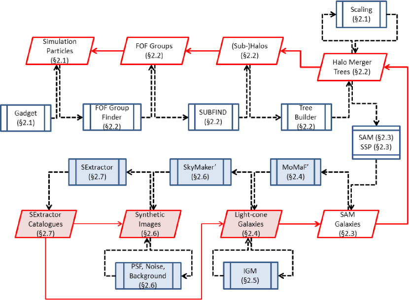
Blaizot et al. (2005) pioneered in the production of realistic artificial telescope data based on lightcones extracted from their semi-analytic model. That paper already laid out most of the workflow that we use here (see Fig. 1): dark matter particle simulations are used to construct halo merger trees on which a semi-analytic model is run. The output from the SAM is used to construct galaxy lightcones that are used as input for artificial telescope image simulations. Galaxies are extracted from the artificial images using standard observational tools (e.g. SExtractor; Bertin & Arnouts, 1996), and the resulting galaxy catalogs are compared to the original simulations at different levels, or to actual observations. Unfortunately, however, the methods of Blaizot et al. (2005) were never employed on a large scale, and in subsequent years the comparison between SAMs and real observations has been mostly performed at the lightcone level or even at the snapshot level, thereby sidestepping many of the details involved in analyzing real telescope data that observers typically have to go through. As we shall show, however, numerous problems in the field of galaxy evolution could benefit from a simulation that accounts for the entire observational process. This leads to new insights involving details that are missed by higher-level comparisons between data and simulations. By expanding on the basic ideas of Blaizot et al. (2005), the MRObs aims at making this possible.
1.3 Why the Millennium Simulations?
Although in this paper we lay out the motivation and framework for producing synthetic data from cosmological simulations in general, the MRObs is based around the suite of MR simulations. Through the combination of simulations volume and particle resolution, an active development of semi-analytic models, and an online database providing access to numerous data products, the MR is ideally suited for most of our purposes, as follows.
(1) Volume and resolution: The MR has an almost ideal combination of volume and particle mass resolution suitable for a wide range of applications. The resolution111Full convergence between the MR and the much higher resolution MR-II simulation is near . is sufficient to identify the halos believed to host faint galaxies at very high redshifts (Ouchi et al., 2005; Overzier et al., 2006), while probing significantly down the stellar mass function with good statistics at lower redshifts. The volume is large enough to probe a very wide range of environments. The MR contains about 3,000 cluster-sized objects at , of which about 25 are of the Coma-type (i.e., more massive than ). The formation of all these systems can be traced back to very high redshift for detailed studies of cluster formation (Overzier et al., 2009a). The large volume is also crucial for constructing synthetic galaxy surveys covering many square degrees without significant replications (Kitzbichler & White, 2007; Guo & White, 2009; Overzier et al., 2009a; Henriques et al., 2012).
More recent dark matter simulations have been performed. The MultiDark simulations span an larger volume but with a lower mass resolution compared to the MR (Prada et al., 2012). The Bolshoi simulations have a higher mass resolution, but are smaller (Klypin et al., 2011). Neither simulation has yet released semi-analytic galaxy catalogs that can be used to compare with actual observations. The somewhat limited mass resolution of the MR has recently been extended by two orders of magnitude through the MR-II simulation (Boylan-Kolchin et al., 2009). This simulation is extremely useful for further improving the semi-analytic model that can then be re-applied to the original MR simulation (Guo et al., 2011). The somewhat limited volume of the MR has also recently been extended by two orders of magnitude through the Millennium XXL (MXXL) simulation (Angulo et al., 2012), useful for studies of the rarest, most massive objects. However, for the generation of mock lightcones, the MR is currently still our preferred simulation ( larger volume compared to the MR-II and higher resolution compared to the MXXL).
Recently, it has become possible to re-cast the suite of MR simulation results in more updated cosmologies relative to WMAP1 thanks to the re-scaling technique of Angulo & White (2010, see §2.1.1).
(2) Semi-analytic models: As we will show, the Guo et al. (2011) semi-analytic model applied to the MR is key to producing our synthetic observations. This model gives detailed predictions for the evolving sizes and spin axes of the stellar mass in disks and/or bulges that are crucial for calculating angular sizes, bulge-to-disk ratios, inclinations and position angles.
(3) MR database: The dark matter and galaxy catalogs of the MR project and related simulations have been made widely accessible to the community through the MRDB (Lemson & Virgo Consortium, 2006). Interested users can query the data in this database through various online services using standard Structured Query Language (SQL). Regular updates to the MRDB holdings provide public access to the latest model results, ensuring that anyone can analyze the MR data and use its results in their publications. We have now added to this system our synthetic imaging data and extracted source catalogs that can be cross-correlated with the underlying simulations data in the MRDB.
In summary, despite the age of the original MR (Springel et al., 2005), more recent dark matter simulations do not yet provide equivalent data sets or the infrastructure required for developing a facility such as the MRObs.
1.4 This paper
In this paper, the first in a series comparing theory and observations in the observational plane, we lay a framework for producing synthetic data from cosmological simulations, describe our main methods for future reference, present a number of user examples, and announce the public release of a large number of simulated surveys (synthetic images and catalogs). We also present various new online services that allow one to interact with the synthetic observations and the underlying lightcones, semi-analytic galaxy and dark matter catalogs in the MRDB. The structure of this paper is as follows. In §2 we will present a concise overview of the MRObs and describe in detail all the steps that are needed in order to go from a pure dark matter simulation and semi-analytic galaxy catalog to producing realistic synthetic observations. In §3 we present a detailed simulations example focusing on our synthetic images produced for the on-going CANDELS HST program. In §4 we illustrate the new types of questions that can be asked of the MRObs through a number of examples related to galaxy and galaxy cluster evolution. In §5 we present the public data release and the interactive online tools we have developed. In §6 and §7, respectively, we present a brief outlook to future developments related to the MRObs project and summarize our results.
2 Structure of the Millennium Run Observatory
The MRObs makes available a fully interconnected set of data products
covering the entire chain from dark matter simulations to synthetic
observations and extracted data. In the MRObs, each subsequent step
uses data products produced by previous steps, and almost all the data
products are available for interrogation and public download for
further analysis. A schematic overview of this process is given in the
workflow diagram in Fig. 1, where rectangles indicate
an action and tilted rectangles represent data products that in each
step can be linked to products
elsewhere along the chain. The main steps are:
1. Dark matter particle simulation (DM density fields)
2. Identifying of friends-of-friends (FOF) groups
3. Identifying (sub-)halos
4. Constructing halo merger trees
5. Applying semi-analytic galaxy models
6. Observing galaxies on a synthetic light-cone
7. Producing synthetic telescope images
8. Extracting sources from synthetic images
In this section we will describe each of the steps in more detail, focusing on the newly developed components that are most essential to bridge the gap to real observations (steps 6–8), and refer to other work for the components described in detail elsewhere (steps 1–5).
2.1 The Millennium suite of dark matter simulations
The evolution of the dark matter distribution with time is believed to be mainly driven by the initial matter power spectrum, gravity, and the expansion rate of the universe, and can be taken either from direct -body simulations (e.g. Davis et al., 1985; Jenkins et al., 1998; Springel et al., 2005), or from (semi-)analytically constructed dark matter halo trees (e.g. Press & Schechter, 1974; Kauffmann & White, 1993; Lacey & Cole, 1994; Somerville & Kolatt, 1999; Sheth et al., 2001; Neistein & Dekel, 2008). In the suite of cosmological simulations centered around the MR project, the dark matter simulation was performed with versions of the cosmological simulation code Gadget (Springel et al., 2005). The suite of simulations consist of (1) a 21603 particles simulation with particle mass and periodic box length of 500 Mpc (Springel et al., 2005), (2) a 21603 particles simulation with mass and periodic box length of 100 Mpc (the Millennium-II (MS-II); Boylan-Kolchin et al., 2009), and (3) a 67203 particles simulation with mass and periodic box length of 3 Gpc (the Millennium-XXL (MXXL); Angulo et al., 2012). All simulations follow the gravitational growth as traced by these particles from to 0 in a CDM cosmology (, , , , ) most consistent with the Wilkinson Microwave Anisotropy Probe (WMAP) year 1 data (Spergel et al., 2003). The dark matter particle distributions were stored at 64 discrete epochs (‘snapshots’).
2.1.1 Scaling of cosmological parameters
The suite of MR simulations were performed using the now disfavored WMAP1 cosmology. While the lower value of preferred by the more recent WMAP7 data will cause the growth of dark matter structure to be delayed with respect to a WMAP1 cosmology, its effect on galaxy formation models is less straightforward to infer. Running simulations with multiple cosmologies is a time-consuming process. Instead, the MRObs project uses a recent technique introduced by Angulo & White (2010) in which the output from a cosmological -body simulation in one cosmology (e.g., WMAP1) can be scaled to represent the growth of structure in another cosmology (e.g., WMAP7). Tests comparing direct -body simulations done in two cosmologies with a simulation that was scaled from one to another cosmology show that power spectra are reproduced to better than 3% at all scales. In the MRObs the technique is applied to halo catalogues. Properties such as mass, concentration, velocity dispersion and spin are scaled are reproduced at about the 10% level or better (Angulo & White, 2010) (see also Ruiz et al., 2011). Guo et al. (2012) give the properties of semi-analytic galaxies in the MR and MR-II scaled to the WMAP7 cosmology.
2.2 Dark matter halos
The MR simulations output the dark matter phase-space distribution at 61 different epochs at . The spacing between these outputs is roughly equal in the log of the expansion factor, specifically, 300 Myr for and 100 Myr for . In each of these snapshots, DM haloes are found using a FOF algorithm (Davis et al., 1985) with a linking length parameter equal to one fifth of the mean inter-particle separation. Within each FOF halo, self-bound substructures are identified using the SubFind algorithm (Springel et al., 2001).
For each subhalo, at each output time, a unique descendant in subsequent snapshots is assigned as the subhalo which contains the majority of the most bound particles (slightly different definitions have been used among the different Millennium simulations). Finally, these pointers are arranged in a tree-like data structure which allows to access the full mass evolution of a given object across time. This structure – a halo merger tree – represents the backbone and starting point for our post-processing simulations of galaxy formation.
2.3 Synthetic galaxy catalogues
2.3.1 Semi-analytical galaxy formation models
The N-body simulations used in the MRObs follow dark matter particles only. To add predictions about the baryonic content of the model universe, we rely on an approach that generally is referred to as semi-analytical modelling (SAM) (e.g. White & Frenk, 1991; Kauffmann et al., 1993; Cole et al., 1994; Kauffmann et al., 1999; Somerville & Primack, 1999; Kauffmann & Haehnelt, 2000; Somerville et al., 2001; Springel et al., 2001; Hatton et al., 2003; Kang et al., 2005; Cattaneo et al., 2005, 2006; De Lucia & Blaizot, 2007; Monaco et al., 2007; Guo et al., 2011; Somerville et al., 2012, and references therein). Using simplified descriptions (‘recipe’) for the baryonic physics, these models follow the evolution of the galaxies within the skeleton provided by dark matter halo merging trees defined in the previous steps. These recipes include gas cooling, star formation, reionization heating, supernova feedback, mergers, black hole growth, metal enrichment and feedback from active galactic nuclei. The recipes are constrained by local observations and by physical insight.
This technique is much less computationally expensive than adding full hydrodynamics to the basic simulations. Once the backbone formed by the dark matter structure has been established, the semi-analytic modeling of the galaxies can be repeated many times in order to find the recipes and parameters that are required to match the observations.
The MRDB (Lemson & Virgo Consortium, 2006) contains galaxy catalogues from two SAMs, L-GALAXIES, created at the Max-Planck-Institute for Astrophysics in Garching (Springel et al., 2001; Croton et al., 2006; De Lucia & Blaizot, 2007; Bertone et al., 2007; Guo et al., 2011), and GALFORM, created by the University of Durham (Cole et al., 2000; Benson et al., 2003; Baugh et al., 2005; Bower et al., 2006). Compared to earlier models, also stored in the MRObs, the latest version of the Munich model by Guo et al. (2011) that we focus on here, includes improved prescriptions for supernova feedback, gas stripping, galaxy merging, and bulge formation (see Croton et al., 2006; De Lucia & Blaizot, 2007; Bertone et al., 2007; Guo et al., 2011; Henriques et al., 2012, for successive versions of the Munich model applied to the MR). The output of the SAM is stored for each of the 64 snapshots, thus sampling the evolution of the galaxy population every few 100 Myr. The SAM calculations, however, are computed on a finer grid consisting of 20 steps of about 10 Myr each between each pair of snapshots. This ensures that the properties of galaxies are modeled on time-scales appropriate for a wide range of star formation histories, including brief bursts of star formation that may happen in between snapshots.
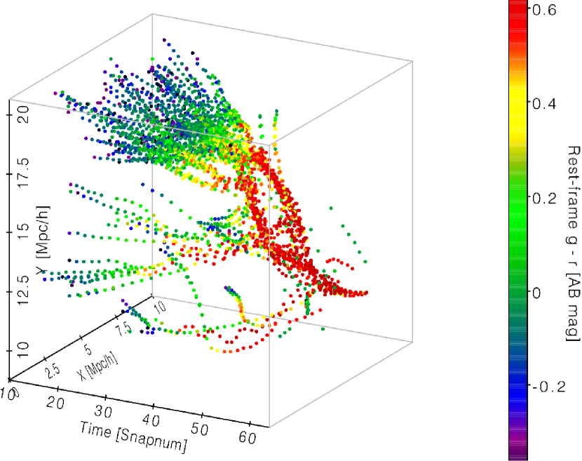
The galaxies resulting from the semi-analytic model naturally span a wide variety in star formation histories (SFHs), corresponding to the different gas accretion and merger histories of individual galaxies. The relational database of the MRObs allows us to reconstruct these SFHs in great detail. It is important to keep in mind the distinction between the SFH of the galaxy that forms the main branch in a galaxy merger tree, and that of the stars in all the progenitors of a descendant identified at some snapshot. As shown by De Lucia & Blaizot (2007) this typically results in large differences between the time it took for the stellar mass to be formed (‘formation time’) and the time it took for that mass to assemble into a single galaxy (‘assembly time’). An example is shown in Fig. 2, showing the stellar populations of all the different branches that form the merger tree of a single galaxy at . When observers study the star formation history of a particular galaxy selected at some redshift, they do thus not necessarily study the SFH of a single galaxy, but rather the SFH of all its progenitors (weighted by stellar mass).
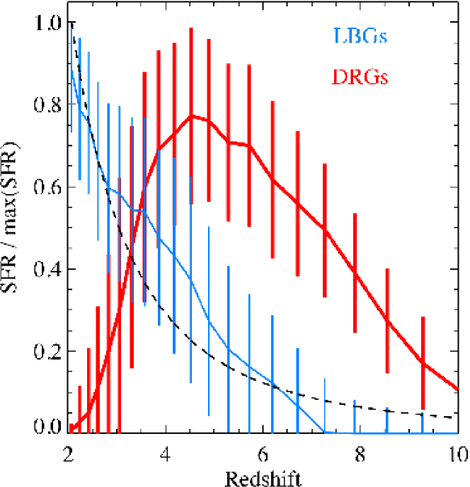
Similar to real galaxies, galaxies in the MRObs span a very large range in SFHs. In Fig. 3 we show the average SFHs for star-forming and quiescent galaxies in the MRObs. These SFHs were determined by summing the SFRs of all the progenitors of 100 galaxies selected at . For systems having SFRs of 10 yr-1 and (e.g., similar to Lyman Break Galaxies, LBGs), the SFHs are rising (blue line in Fig. 3), roughly as derived from observations of LBGs (Papovich et al., 2011). For systems having SFRs of 10 yr-1 and (e.g., similar to Distant Red Galaxies, DRGs), the average SFH rapidly declines after (red line) analogous to the best-fit SFHs of DRGs observed (e.g. Kriek et al., 2006).
2.3.2 Multi-wavelength model predictions
SAMs predict physical properties of galaxies, such as their stellar masses, ages, metallicities, and gas content. One common way of testing the models is to compare them to the same physical properties derived from the SEDs of observed galaxies. At the least, this approach depends on having well-established measuring techniques and accurate stellar population synthesis models (see Tinsley, 1980). In practice, this sort of analysis typically includes numerous assumptions, and certain features of the galaxies can never be recovered from the observations in full (e.g., their exact star formation history or dust attenuation). In the MRObs the application of stellar population synthesis models and dust recipes allow one to make detailed spectro-photometric predictions for the model galaxies by adding up synthetic spectra corresponding to the different generations of stars that these galaxies consist of at any moment. The great predictive power of SAMs in terms of the observable, photometric properties of galaxies is in large part based on the spectral synthesis modeling of the stellar populations being formed in the semi-analytic model galaxies according to their SFRs at any given time (see Fig. 2 for an example of a typical galaxy).
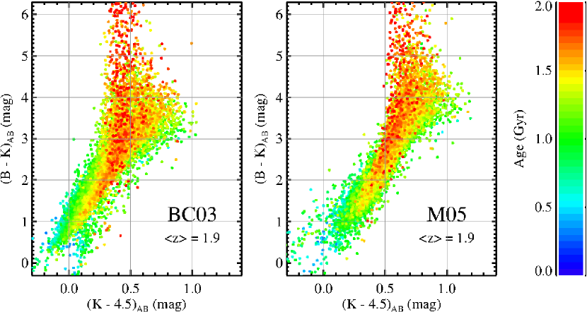
The predicted multi-wavelength properties of galaxies depend on the spectral synthesis model used. These models are currently still affected by gaps in our understanding of stellar evolution (e.g., see Conroy et al., 2009), preventing us from making unambiguous predictions for the main galaxy observables. Two well-known synthesis models implemented in the MRObs are those by Bruzual & Charlot (2003, ‘BC03’) and by Maraston (2005, ‘M05’). These models are illustrated in Fig. 4, where we show the observed –4.5m vs. – colour-colour diagram for galaxies at in our simulations. The M05 model shown right predicts significantly redder colours compared to the BC03 model shown left, especially for galaxies between 1 and 2 Gyr in age (for discussion, see Tonini et al., 2010; Henriques et al., 2011, and references therein).
We model the effect of dust on the predicted colours and magnitudes using the dust treatment recipe detailed in Guo & White (2009) (see also De Lucia & Blaizot, 2007; Kitzbichler & White, 2007; Guo et al., 2011; Henriques et al., 2012), and we note that in calculating the extinctions, a random inclination was assigned to every galaxy to determine the extinction relative to the face-on value (assuming a slab geometry). It is important to note that the dust modeling in semi-analytic models is currently performed in a highly simplistic manner. Even though models have shown to be fairly successful in reproducing the overall colours of the evolving galaxy population in some bands, a more realistic treatment of the effects of dust could easily alter the spectral energy distributions of certain galaxies at any given time significantly.
The significant uncertainties in the stellar population synthesis models and the dust modeling techniques limit us in producing accurate models of the real universe. For the same reasons, however, they also limit our ability to derive exact physical quantities from real observations. At the very least, the MRObs will thus allow one to test the accuracy of current techniques designed to extract physical quantities from a given set of broadband magnitudes. In the future, the highly modular approach of the MRObs (see Fig. 1) will make it straightforward to add alternative or improved models.
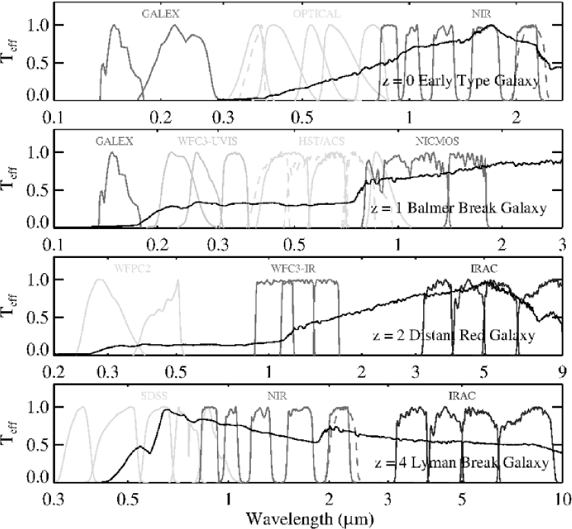
In the current version of the MRObs, the SFHs, stellar synthesis models, and dust extinction models mentioned above are used to generate multi-wavelength filter catalogs (see Henriques et al., 2011, 2012). These catalogs cover the FUV to the mid-IR as observed by major telescopes and instruments (Table 1). The filter bandpasses are illustrated in Fig. 5.
2.4 Lightcone construction
The snapshots of data (in time or in redshift) that are produced by numerical simulations present an idealized view of the evolving universe that is different from data resulting from observations of the extra-galactic sky. In order to allow for more realistic and direct comparisons between the model predictions and observations, we construct so-called ‘lightcones’ in which galaxies that were simulated at discrete snapshots are re-arranged in order to mimic the relation between the distance along an observer’s line of sight and cosmic time as accurately as possible (e.g., see Hamana et al., 2001; Blaizot et al., 2005; Kitzbichler & White, 2007; Sousbie et al., 2008; Guo & White, 2009; Overzier et al., 2009a; Teyssier et al., 2009; Carlson & White, 2010; Henriques et al., 2012).
In this paper we use lightcones introduced in Henriques et al. (2012), to which we add structural properties, and a set of new lightcones pointed at specific objects. These lightcones were built using a version of the Mock Map Facility (MoMaF) code of Blaizot et al. (2005). Because of its importance to the MRObs, here we give a short review of the technique, and describe a use of MoMaF that allows us to create lightcones aimed at specific objects of interest in the simulations and which is specially developed for the MRObs.
2.4.1 Summary of our lightcone method
The MR predicts the detailed properties of the dark matter and the galaxies it contains for a closely spaced set of snapshots that are sufficient to compare with observations from to the highest redshifts currently observed. In principle the simulations box probes a sufficiently large volume to construct large pencil beam surveys. For example, the total simulations volume of (500 Mpc)3 is equivalent to that probed in a pencil beam survey out to and measuring 4 square degrees on the sky. On the other hand, the co-moving distance to of 7,000 Mpc is much larger than the side of the simulations box of 500 Mpc (900 Mpc when taking the diagonal through the box).
Blaizot et al. (2005) suggested ‘replicating’ the simulations box along an artificial observer’s line of sight until the maximum co-moving distance desired is reached, and then extracting a conical pencil beam out of the enlarged volume. They explain that care must be taken to avoid ‘perspective effects’ caused by replication of the same part of the universe in certain directions. Whereas Blaizot et al. (2005) solve this by adding random rotations and translations of the boxes, thereby introducing discontinuities in the galaxy distribution, Kitzbichler & White (2007) showed that for certain orientations of the lightcones through the MR box and for a small enough opening angle of the cone, the lightcone can be constructed without passing through any region of the simulations twice (or at least ensuring that copies are widely separated in redshift if replication occurs). It is the latter method that we use for all pencil-beam light cones in the MRObs.
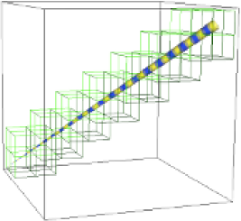
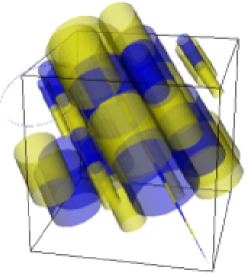
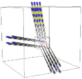
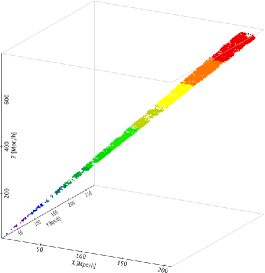
We illustrate the box-replication process in Fig. 6. In the panel on the left, a virtual lightcone is drawn in a much enlarged MR volume constructed using the box replication method. The opening angle of the cone, its origin and angles of intersect with the original MR box are chosen such that every cone segment (indicated by the blue-yellow segments) can be extracted from the original MR volume in such a way as to almost cover the complete simulation volume and without passing through any region of the box twice (as illustrated in the middle panel). Many pencil beam surveys can be constructed from the MR by changing the angles or the origin of the cone (right panel).
Besides these geometric considerations, one must take special care that each galaxy is seen at the evolutionary phase and with the photometric properties corresponding to its redshift along the lightcone. In the MR, snapshots are separated by 100–400 Myr, meaning that the evolving galaxy population is sampled at fairly frequent intervals out to very high redshifts. Fig. 7 illustrates how we connect data from many individual snapshots to obtain an evolving galaxy population as a function of co-moving distance (or redshift) along the lightcone. Each section consists of those galaxies having redshifts , where is the redshift corresponding to snapshot . The physical properties that these galaxies have are then also those they have in snapshot . Because the large-scale structure does not evolve rapidly between snapshots, it is safe to neglect any changes occurring in the distributions of galaxies. However, due to the relatively sparse number of snapshots, especially at very high redshifts, one has to be aware of the fact that there may be discontinuities or ’jumps’ in the absolute numbers of sources as one moves from one lightcone section to the next. The physical properties of the galaxies can also fluctuate heavily between snapshots, but as long as one is interested in the evolution of the global population this can be safely ignored (Kitzbichler & White, 2007). However, in order to ensure that ‘observed’ galaxy properties are correctly related to redshift we perform small interpolations of the observed-frame magnitudes, shifting each galaxy in both redshift and luminosity distance from the snapshot corresponding to redshift to the redshift at which it actually appears on the lightcone (Blaizot et al., 2005; Kitzbichler & White, 2007). In addition to this step, we make corrections to the observed magnitudes due to absorption by the IGM (see §2.5).
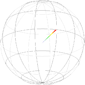
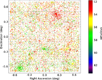
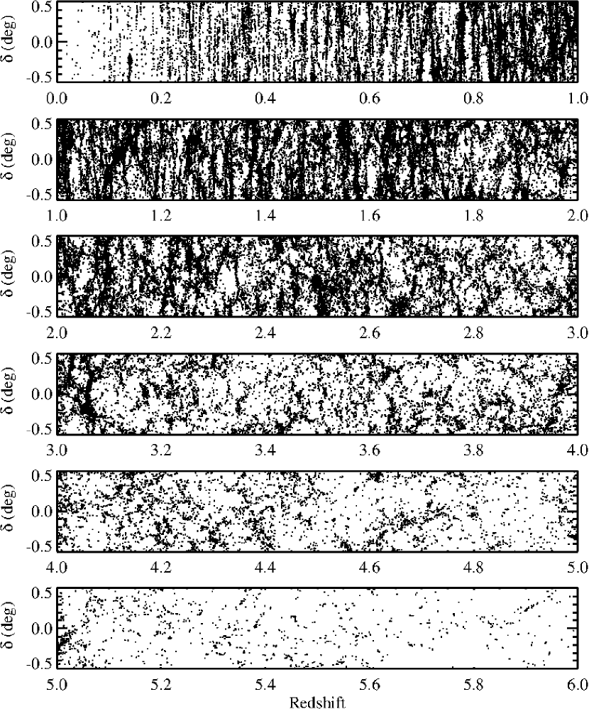
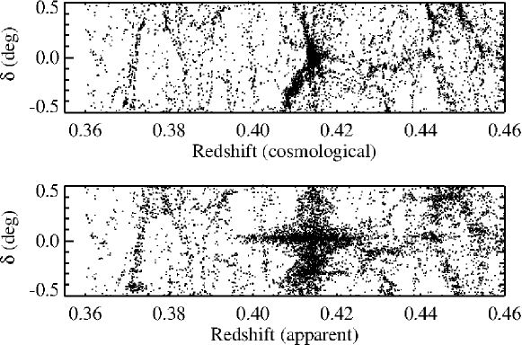
The final step required is to project the cone onto a virtual sky seen by a fictitious observer placed at the center of the celestial sphere (middle panel of Fig. 7). It is now straightforward to assign WCS coordinates (right ascension and declination) to every object in the cone (see Kitzbichler & White, 2007). The projected large-scale structure can be seen in the sky distribution of galaxies plotted in the right-hand panel of Fig. 7. Now that we know both the sky coordinates and the redshifts to every object along the lightcone, we can show the details of the large scale structure that would be probed in a deep pencil beam survey as it would appear in a large galaxy redshift survey out to . In Fig. 8 we plot the redshifts of objects versus their declination on the sky for one of the Henriques et al. (2012) lightcones. Points represent galaxies having -band magnitudes brighter than 26.5 (AB) mag.
2.4.2 Aiming at a specific object
We have made a small modification to the MOMAF code that allows for the construction of lightcones not only in arbitrary directions as described above, but to also ‘aim’ a lightcone such that it crosses through a specific point of the MR box at a specific co-moving distance (or redshift) from the origin. This new technique enables us to model observations toward specific objects or regions by choosing a location within the simulations volume at one redshift and ‘observing’ it within a lightcone with origin at another redshift. Obvious uses of this technique are to study the appearance of a particular galaxy cluster selected at and observed at , or to study the descendant of a halo (or galaxy) selected at . It is important to take into account the peculiar velocities of galaxies when constructing the lightcones as they can heavily distort the observed redshift distributions, especially in the vicinity of massive objects such as galaxy clusters (see Fig. 9).
The MRDB allows one great flexibility in selecting such targets, and even allows one to the define the complete geometry of the light cone in a single SQL query. Our new lightcone aiming technique thus greatly enhances the application of the MR to numerous new problems. Examples related to galaxy clusters will be shown in §4.2.
2.4.3 Inclinations and position angles
One of the unique features and key science drivers of the MRObs is that it aims to produce detailed predictions for the observed galaxy population without having to make assumptions that are not supported or naturally accounted for by the model. The SAMs included in the MRObs allow us not only to predict morphologies and sizes of galaxies, but also their inclinations and position angles as seen by a virtual observer. The latter are derived from the orientation of the galaxy as defined by the angular momentum vector of its stellar disk. The SAM that we use here tracks the change in the total angular momentum vector of both gas and stellar disks. New gas condensing within a halo is assumed to carry the specific angular momentum of that halo. The total angular momentum change of gas disks in each time step is the sum of the change in angular momentum due to gas condensation, gas accretion and gas that is transformed into stars. The change in total angular momentum of stellar disks is given by the change in angular momentum due to gas that gets transformed into stars in each time step.
As a consequence, the SAM predicts not only the spatial positions but also the orientations of all galaxies with respect to the three-dimensional, co-moving, Cartesian coordinate system of the simulation box. From this we can then calculate the observed inclinations and position angles of each galaxy based on the angles between the line of sight of our lightcone and the simulation box. Our method ensures that the orientations of galaxies in the MRObs are, at the very least, physically motivated. This allows one to study in detail if the MR predicts any observable correlations between the orientations of galaxies, their parent halos or the large-scale structure. Such models are also suited for, e.g., conducting completeness tests as a function of inclination, for testing galaxy structure decomposition codes, and for paving the way for more elaborate, orientation-based dust screening models that may be implemented into the SAM at a later stage.
2.5 IGM absorption models
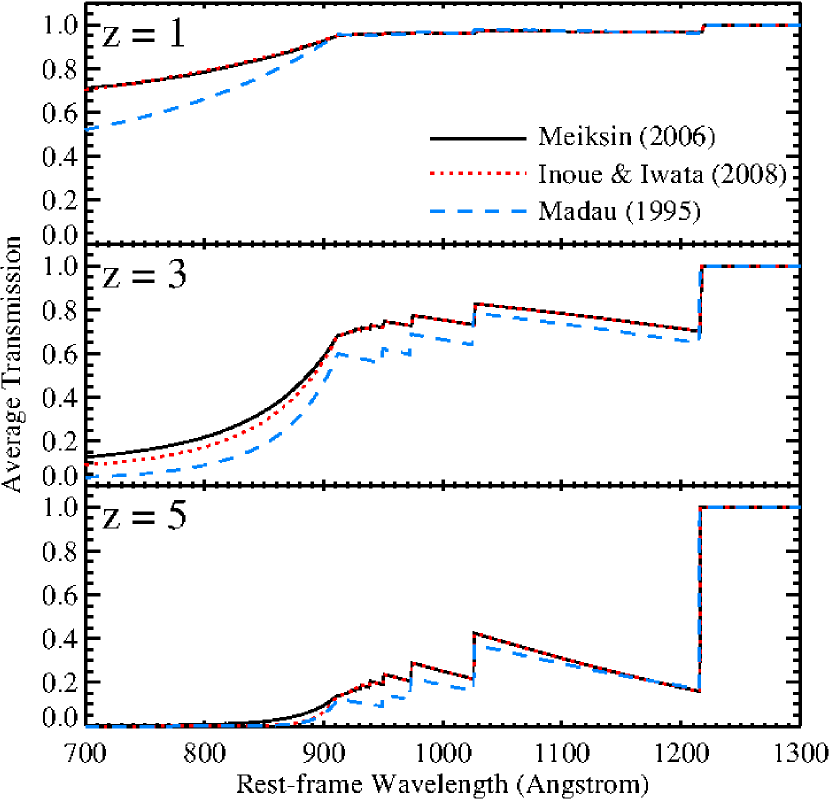
The spectra of galaxies short-ward of 1216 Å in the rest-frame are primarily affected by photoelectric absorption by the neutral hydrogen associated with damped Ly absorbers (DLAs), Lyman Limit Systems (LLSs), optically thin systems, and resonance line scattering by the Ly forest along the line of sight222In our model approximations we neglect the much smaller contribution from intergalactic metals and He absorption.. This absorption affects the magnitudes and colours of galaxies observed in bands corresponding to these rest wavelengths. The strength and shape of this so-called ‘Lyman Break’ depend on the redshift of the source, the intrinsic source spectrum, and the distributions in redshifts and optical depths of the absorbing systems. In order to ensure that these effects are properly accounted for in the MRObs lightcones, at least in a statistical manner, we have implemented three different models for the IGM absorption. We include two models based on the recent IGM transmission calculations by Meiksin (2006, ‘MEIKSIN’) and Inoue & Iwata (2008, ‘INOUE-IWATA’) that are conveniently made available in code form by Harrison et al. (2011, IGMtransmission). We also include the IGM transmission model of Madau (1995, ‘MADAU’) that is still the most widely used in the literature today even though it has been shown to significantly over-predict the absorption in the 912–1216Å range compared to the updated models (e.g. Bershady et al., 1999; Meiksin, 2006; Inoue & Iwata, 2008).
For an intrinsic galaxy spectrum , the attenuated spectrum observed will be of the form , where the effective optical depth of the IGM transmission function can be taken from any of the three IGM models. In Fig. 10 we show the mean transmissions for sources at different redshifts. The MADAU model implies significantly less transmission than the other models.
In the current release of the MRObs, the IGM absorption correction is calculated only after the filter magnitudes are computed. We approximate the spectral shape within the filter response with that of a 100 Myr old, continuously star-forming, solar metallicity stellar population modeled using Starburst99 (Leitherer & Heckman, 1995). For most practical purposes (i.e. in the case of galaxies with significant far-UV emission from a young stellar population), this is a reasonable assumption, and we note that the same assumption is typically made by observers when interpreting the broad-band colours of high redshift dropout galaxies (e.g. Bouwens et al., 2003). In any case, the corrections do not significantly change when assuming a 3 Myr old instantaneous low-metallicity starburst model (0.05 mag change). Although refinements to this method will become available in the MRObs in the future, users can already also apply their own IGM corrections directly on the unattenuated lightcone catalogs that we provide and then use these as the basis for their own image simulations. Because the inclusion of the IGM attenuation is so important for creating realistic mock catalogs and images in the MRObs, a brief review of the MEIKSIN, INOUE-IWATA. and MADAU modeling recipes is given in Appendix A.
2.6 Construction of the virtual telescope data
2.6.1 Galaxy models
Now that we have obtained all the necessary information pertaining to the positions, sizes, viewing angles, bulge-to-disk ratios, and IGM-corrected magnitudes across different filters, we can populate simulated images with galaxies. We follow a two-step process. First we simulate noise-free galaxy profiles projected onto a 2D image plane at very high pixel resolution using a modified version333We optimized Skymaker for dealing with very large input lists in .csv format provided by the MRDB, and for generating extremely large images. of Skymaker (Bertin, 2009). We will refer to the result of this process as the ‘perfect’ or ‘pre-observation’ image. Once the perfect image has been made, it is straightforward to apply all the observational effects such as the PSF, binning, sky background, and noise for any type of observation. This last step is done using our own custom code444Although Skymaker was specifically designed to handle point spread function convolution, sky backgrounds, and simulating detector noise, for various practical reasons we do not currently make use of this functionality but use our own custom IDL and Python codes for these steps of the simulation..
In line with the Guo et al. (2011) semi-analytic predictions, galaxies in the MRObs are composed of an exponential profile for the disk (D) and a De Vaucouleurs profile (S) for the bulge (if any), each having a surface brightness profile in mag arcsec-2 given by:
| (1) | |||||
| (2) | |||||
where is the total magnitude (mag), is the bulge-to-total ratio, is the bulge half-light radius (arcsec), and the disk scale height (arcsec). Skymaker builds these profiles as elliptical shapes at pixel position , projected on the sky with position angle and inclination according to (see Bertin & Arnouts, 1996):
| (3) |
such that the algorithm for calculating the projected light profiles for disks and bulges becomes:
| (4) |
with
and are the projected major and minor axes, with for disks and for bulges, and with the projected aspect ratio of the system.
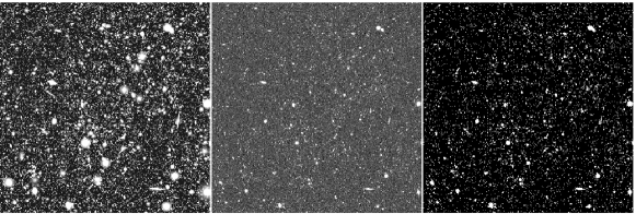
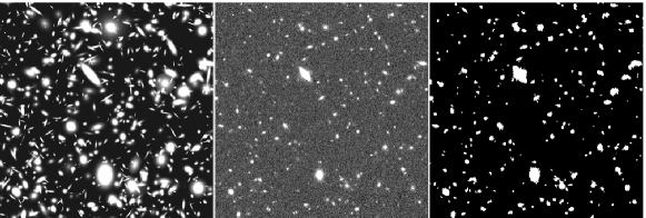
Our modified version of Skymaker performs this process efficiently for typical MRObs simulations that are based on lightcones containing several millions of galaxies per square degree. An example of the ‘perfect image’ produced is shown in the left panel of Fig. 11, where the white shapes indicate the simulated galaxy images. The corresponding final (‘noisy’) telescope image produced following the process detailed below is shown in the middle panel.
2.6.2 Input parameters: positions, magnitudes, inclinations, orientations, sizes, and bulge-to-disk ratios
The center positions of all objects in the image plane are determined from the right ascention and declination relative to the lightcone centres and the pixel scale of the desired instrument. Inclinations and position angles are uniquely determined from the angular momentum vector of the stellar disks relative to the orientation direction of the lightcones through the MR volume (Fig. 6). Angular sizes are determined from the physical size and the diameter distance, , at the redshift of each source in the lightcone.
We list the specific parameters required by Skymaker for simulating each galaxy, and give a brief explanation of how this parameter follows from our models.
-
•
, : The source position in image pixel coordinates. This position is defined by the sky coordinates of a galaxy in the lightcones, the desired pixel scale of the image, the field of view, and the position of the image center relative to the lightcone center.
-
•
: The total apparent (AB) magnitude of the source in the desired filter. This magnitude includes the attenuation by dust as well as the IGM absorption.
-
•
: The bulge-to-total ratio of the source. This parameter, for which we take the ratio of the fluxes predicted for the bulge and total in each filter, is needed for assigning magnitudes to the bulge () and disk () components.
-
•
: The scaleheight of the disk in arcseconds. This is defined by stellardiskradius, with stellardiskradius taken from the Guo2010a..MR table555The Guo2010a..MR table stores the galaxy catalogue obtained by applying the SAM from Guo et al. (2011) to the MR halo merger trees. in the MRDB and is in units of kpc.
-
•
: The equivalent (or half-light) radius of the bulge measured in arcseconds. This is calculated as bulgesize, where bulgesize is taken from the Guo2010a..MR table and is in units of kpc.
-
•
: The projected aspect ratio of the disk that is uniquely determined by the angles of intersection of the lightcone with the MR volume and the intrinsic spin axis of the galaxy stellar disk.
-
•
: The position angle of the disk, defined by the angles of intersection of the lightcone with the MR volume and the intrinsic spin axis of the galaxy stellar disk.
-
•
: The projected aspect ratio of the bulge. Because all bulges in Guo et al. (2011) are spherical, we set this value to 1.0.
-
•
: The projected aspect ratio of the bulge. Because all bulges in Guo et al. (2011) are spherical, we set this value to 0.0.
2.6.3 The virtual telescope model (sky, PSF, noise, and all that)
The MRObs produces realistic telescope data by applying an ‘observation description’ (OD) to the perfect image created in the previous step. The OD consists of a set of instructions that completely defines a particular observation to be mimicked, e.g., telescope, detector, filter, exposure time, number of sub-exposures, dither strategy, and sky conditions. Although the exact modeling method may vary depending on the details of a specific instrument or survey, here we list the basic observational effects typically being added in sequence:
(1) The first step is to scale the perfect image populated by our bulge+disk surface brightness simulations to their proper fluxes measured in detector electrons by multiplying the models in Eq. 2.6.1 by the factor
| (5) |
where is the AB magnitude of the disk/bulge, ZP is the zero-point in AB magnitudes that gives a detector count rate of 1 ADU , the image exposure time in seconds, is the detector gain in ADU-1, and and are the coordinates of pixel belonging to each source.
(2) We add a sky background. The value of the background is usually kept constant across the field (we use gnomonic projections) based on the average conditions at a particular site or telescope, or is based on the sky background level measured in a particular survey that is being modeled.
(3) The image is convolved with a point spread function (PSF). The PSF can have various origins: it can be taken from a PSF simulator (e.g. TinyTim in the case of HST), from (a stack of) stars extracted from a fully reduced observation, or modeled with a simple function (e.g., a Gaussian).
(4) The image is rebinned to the desired pixel scale. If the PSF is taken from an actual observation and is not available at sub-pixel resolution, the rebinning step is performed before the PSF convolution step.
(5) Detector dark current is added to the image.
(6) Poisson noise is calculated for each pixel value.
(7) Gaussian-distributed readout-noise is added.
(8) WCS astrometry is added to the image header based on the pixel scale and the astrometric system of the lightcone.
(9) Scientific images in .fits format are created, optionally with corresponding background and noise maps. Complex observations having the proper noise characteristics can be created from co-adds of multiple exposures made following the same above procedures.666Although the original version of Skymaker is capable of simulating bleeding, blooming and saturation, we do not currently include these effects for practical purposes. However, we do release the object input lists and the ‘perfect’ images for all our simulations (§5), such that interested users can perform their own modeling of these (or other) effects.
2.6.4 Galactic extinction and stars
Optionally, we apply Galactic foreground extinction to the input galaxy models by specifying the amount of reddening in units of and assuming the Cardelli et al. (1989) attenuation curve with . If desired, Galactic stars can be added to the image, either based on a user-specified input distribution or based on an accurate Milky Way model (e.g., TRILEGAL; Girardi et al., 2005).
2.7 Source extractor
With the synthetic images produced in the previous section, it is straightforward to analyze the data analogous to real observations. Sources in the images are detected by using the Source Extractor (SExtractor) software (Bertin & Arnouts, 1996), which efficiently decomposes a pixel image into ‘objects’ detected at some specified threshold of flux above the image background. Photometry and other basic measurements are performed on all the detected objects yielding a source catalog corresponding to the image. The exact way in which objects are defined and how measurements are performed depend on the setting of various of the parameters in SExtractor, while the total number of objects that can be recovered from the image and the errors on their photometry largely depend on the image quality itself. The MRObs makes it convenient to test the different detection and photometry techniques available in the literature, especially because the properties of the galaxies that were used to create the mock image are exactly known (as opposed to galaxies in real observations).
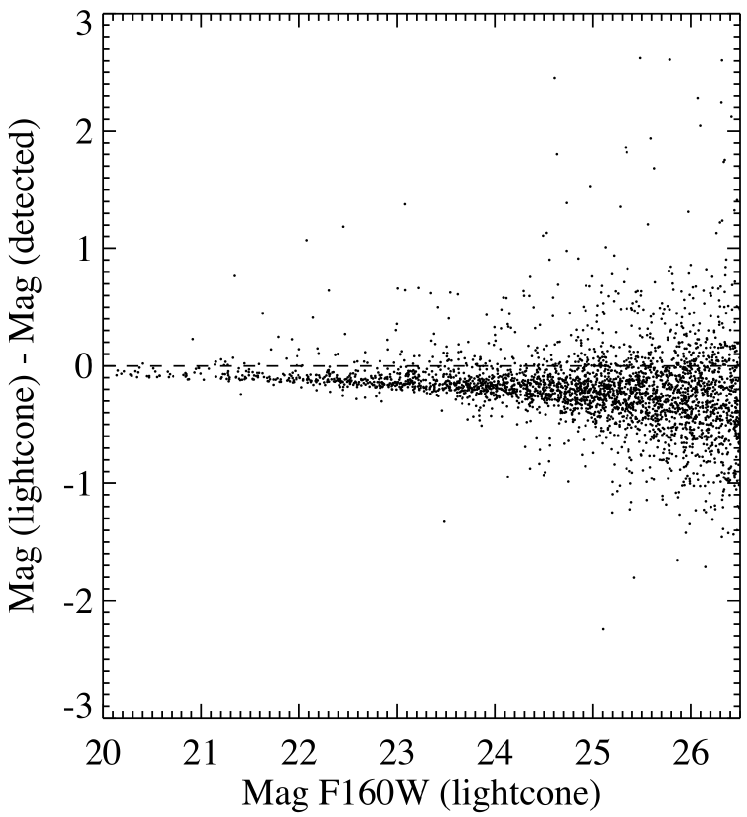
We have run SExtractor on the mock HST/WFC3 -band image shown in Fig. 11 (middle panels). Panels on the right show the SExtractor ‘segmentation image’, indicating all the objects that were detected in the mock image. While there is good correspondence between the two (nearly all objects seen in the mock image are also seen in the detection image), the perfect (input) image shown on the left contains many more galaxies, most of which are too faint to be detected in the mock observation. By cross-correlating the positions of detected objects listed in the SExtractor output catalogs with the positions of objects in the underlying lightcone (both available in the MRDB), we can find out which of the semi-analytic galaxies (identified by their GALAXYID) were detected in the image. This enables us to perform various diagnostic tests between measurements extracted from the synthetic observations and the corresponding intrinsic physical properties from the lightcone. One such test is to study how well the real magnitudes are recovered from the synthetic images by SExtractor. In Fig. 12 we show a so-called ‘trumpet’ diagram indicating the difference in magnitude between the ‘true’ input value and the total magnitude given by SExtractor. The test shows, quantitatively, both how the amount of flux lost due to missed light, and how the photometric scatter due to increased noise increases toward fainter magnitudes.
Because the cross-match between the SExtractor catalog and the lightcone catalog gives us the GALAXYID of each galaxy in the images, this provides us also with a direct link to all the available physical quantities in the semi-analytic snapshot catalogs, the dark matter halo catalogs, and the underlying dark matter density fields, such that it becomes possible to perform numerous experiments related to how well we can extract such physical parameters starting from any kind of observation that can be modeled using the MRObs.
3 Example: simulating CANDELS data
Large extra-galactic surveys often have complicated tiling patterns, exposure time variations, and masked regions across their total field of view that complicate the analysis. It can be convenient to include these kind of effects into the image simulation. This ensures that the signal-to-noise properties and the geometriy of the real and mock data sets are comparable. Here we will illustrate the technique that we use to accomplish this by performing a mock image simulation of the ongoing multi-cycle treasury program Cosmic Assembly Near-Infrared Deep Extragalactic Legacy Survey (CANDELS; Grogin et al., 2011; Koekemoer et al., 2011, HST Programs 12060–12064, 12440; PI: S. M. Faber) that primarily observes with the WFC3 on HST.
3.1 The CANDELS observations
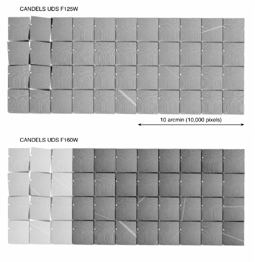
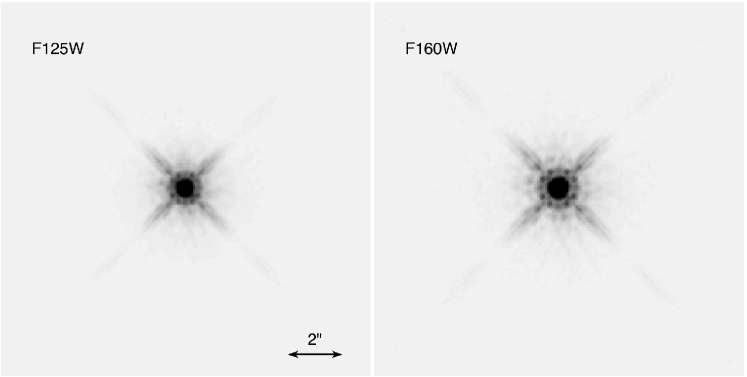
Part of the ongoing HST CANDELS program, the UKIDDS Deep Survey (UDS) field measures approximately 23′10′ in the filters F125W () and F160W (). This field of view is covered with 44 individual pointings with HST/WFC3 resulting in the tiling pattern shown in Fig. 13. For each tile, four exposures were obtained in both filters, resulting in average total exposure times across the field of 1900 s in F125W and 3300 s in F160W. The data were combined onto a common output frame measuring about 22,00010,000 pixels with a pixel scale of using the MULTIDRIZZLE software (Koekemoer et al., 2003; Fruchter et al., 2009). The resulting PSF in the drizzled data measures 012 (F125W) and 018 (F160W) in FWHM (Fig. 14). How well can we simulate these kind of data based on cosmological simulations using the MRObs?
3.2 The CANDELS simulation
Using the procedures outlined in §2.6 we can produce highly accurate mock ‘CANDELS’ data in a number of complementary ways.
(1) The first and most cumbersome method would be to produce each individual CANDELS tile at the correct telescope position and roll angle, and then to process the entire data set through MULTIDRIZZLE analogous to the processing performed on the real data. While this is certainly possible, for many scientific applications a good match between the simulated and real data sets can already be obtained by side-stepping the laborious drizzling process.
(2) The simplest and most straightforward way is to directly generate mock images the size of the entire UDS field based on our model for the HST/WFC3 camera, the main UDS survey parameters, and a mock lightcone as input. This method produces mock UDS images for which the properties (e.g., noise, resolution) are, on average, very similar to those of the real survey. This is an extremely fast method for generating mock data sets that are approximately similar to the observations that are being modeled. It is also a powerful method to simulate images for a survey that has not (yet) been performed, or for simulating a survey at an arbitrary depth or field size.
(3) Our third method, the one that we will use for our demonstration, is an extremely powerful technique for generating a more precise simulation in which the pixel-to-pixel noise variations and geometry of the simulated images can be exactly matched to those of the real data. For this method we make use of ‘weight maps’ associated with the science data for many surveys. The CANDELS UDS weight maps (shown in Fig. 13) record the inverse variance of each pixel calculated during the image reduction process (Koekemoer et al., 2011). The HST inverse variance images (in units of ) are usually calculated as follows
| (6) |
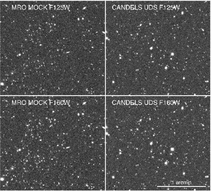
where is the inverse flat-field, is the exposure time, is the accumulated dark current, is the accumulated background, and is the read-out noise (Koekemoer et al., 2011). The weight map includes all sources of instrumental and background noise, but not that of the science objects themselves to allow proper photometry with tools like SExtractor. As a first step we therefore produce simulated images that include the PSF-convolved objects (including the Poissonian object noise) but not the simulated background and read-noise we would normally apply. Instead, we add in these sources of noise by directly taking them from the inverse variance maps. As a final step we need to take into account that in the real CANDELS images the noise is spuriously correlated as a result of the drizzling process used to combine the many individual exposures. The amount of noise correlation depends on the multidrizzle parameters, which for the CANDELS UDS data amounts to a pixel rms noise reduction of a factor of 2 (Casertano et al., 2000). We introduce this noise correlation in our mock images by smoothing the mock images with a small Gaussian kernel (of about 1.5 pixels FWHM, in this case).
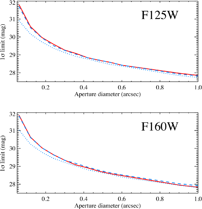
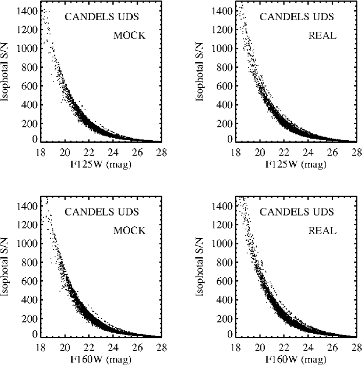
In the left panels of Fig. 15 we show a portion of the final simulated CANDELS images in the filters F125W and F160W. In the panels on the right, we show a region of the real CANDELS UDS images, displayed at the same zoom level and at the same colour stretch as the mock images shown on the left. At a qualitative level the images are remarkably similar. Note that this is not only the result of our accurate image simulation technique, but also because our input galaxy population apparently has a striking resemblance to the observed one (e.g., in terms of number density, clustering, size and shape distributions, and brightness). However, before we can compare the galaxy populations in the simulated and the real data, we need to ensure that the image properties of our simulated data are indeed quantitatively similar to the real data. In Fig. 16 we show the measured background noise fluctuations as a function of aperture diameter as measured in the real CANDELS images (red solid lines) versus that measured in our simulated data set. The blue dotted lines indicate the (true) noise level in the absence of correlated noise. When we introduce the correlated noise resulting from the drizzling process, we get a near perfect match between the simulated (blue dashed lines) and real (red solid lines) CANDELS UDS images. As a second test, we look at the distribution of signal-to-noise (S/N) for objects detected in the real and simulated images. We ran SExtractor using identical detection parameters on the real and simulated images, and plot the isophotal S/N versus the measured magnitudes. The result is shown in Fig. 17 for the mock data (left panels) and the real data (right panels). Again, the S/N distributions are very similar between the real and simulated data, indicating that our image simulations are accurate.
In §4.1 we show an application of these CANDELS simulations by comparing the galaxy number counts in our semi-analytic mock lightcones with those extracted from our mock images, and with those in the real CANDELS images. The simulated CANDELS data produced here are part of our first scientific data release as announced In §5.
4 Examples of applications
4.1 Galaxy number counts in CANDELS
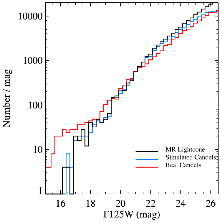
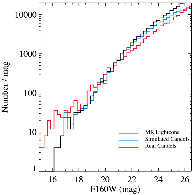
One of the most basic tests that are used to test the accuracy of semi-analytic model predictions is to compare the number counts of galaxies observed as a function of apparent magnitude in some band with those predicted by a mock lightcone observation constructed from the semi-analytic model as described in §2.4. However, as discussed in the introduction, these light-cones do not suffer from any of the observational effects afflicting real observations.
The MRObs approach to modeling discussed in sections 2.5 to 2.7 allows us to make comparisons between observations and semi-analytic predictions in a highly realistic way. By simulating a mock survey matched to the real observations that one wants to compare with, and then running source extraction and photometry software on the mock and real images in identical manner, we can in principle assess how certain observational biases affect the interpretation of the real data, and how this impacts on our comparison of those real data with the simulations. Of course, one has to be aware that other biases may be introduced simply due to the fact that the models are likely no perfect match to the real data.
As a first example, we compare the number counts measured from a mock lightcone to those derived from our mock images based on that lightcone. Fig. 18 shows the two types of number counts from our simulated CANDELS UDS data in blue compared to the plain light cone data in black. The counts extracted from the simulated image were not corrected for completeness. At bright magnitudes ( mag) the counts are in good agreement, but they diverge toward fainter magnitudes counts detected in the images compared to the lightcone on which the mock images are based. The extracted counts are about a factor of 2 lower than the lightcone counts at mag.
The red lines in the figure show number counts measured in the real CANDELS UDS data (no completeness corrections applied). At the faint end, the lightcone substantially over-predicts the observed counts, similar to discrepancies between semi-analytic predictions and observations found in earlier studies. However, it is very interesting to note that the difference between the semi-analytic predictions and the real number counts becomes smaller when we compare the real data to our mock data. Simply by ‘observing’ the lightcone we already lose a significant number of galaxies that would not be detected in a real observation (if the lightcone was an accurate reflection of reality).
The results presented in Fig. 18 suggest that it is important to take observational effects into account when comparing real data with simulations. These effects need to be quantified before one can change the parameters in a semi-analytic model to better match the observations. With the mock data produced by and published through the MRObs these tests can now be performed easily. A more detailed analysis of the number counts in synthetic observations as predicted by the MRObs compared to those predicted by ordinary semi-analytical models will be presented in a follow-up paper.
4.2 The properties of galaxy clusters at low and high redshift
Our new lightcone ‘aiming’ technique described in §2.4.2 offers an efficient way for predicting the detailed observational properties of, for example, galaxy clusters. Here we present mock SDSS and HST observations of a massive galaxy cluster at different redshifts and orientations. The cluster was selected from the roughly 3,000 clusters in the MR, and has a total dark matter mass of at . The selection was performed using the table of friends-of-friends groups in the MRDB. After finding FOF groups in the right mass range, a random selection was made of a cluster. That cluster was traced backwards in time using the table with halo merger trees. At desired redshifts the position of the cluster’s main progenitor was returned. That position, together with a direction and using the co-moving distance corresponding to the redshift, was used to define a light cone that had the cluster at its center and at exactly the correct redshift. This cone was then observed using a few different virtual telescope configurations.
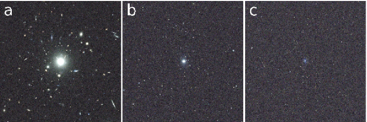
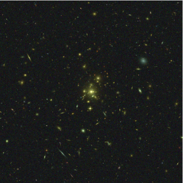
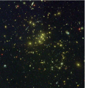
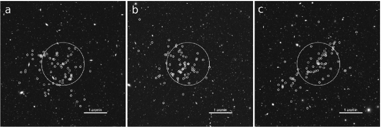
In the first example, we have produced mock SDSS images in showing what this cluster would look like at redshifts from to (Fig. 19). These mock data can be compared directly with real clusters found in the SDSS. It is clear from Fig. 19 that the study of galaxy clusters in the SDSS survey becomes challenging already at moderately high redshifts. As a second example, we therefore show a mock image of the same cluster, now seen at and observed with HST/ACS in the filters (Fig. 20, left panel). In the right panel we show an actual HST image of the well-studied cluster Cl0024 with a comparable dark matter mass (Jee et al., 2007; Harsono & De Propris, 2009). The images were produced using identical parameter settings in the software that produces the colour images from the .fits files (see §5.4.1). Although both clusters have a dominant population of red sequence galaxies that appear almost identical in these HST/ACS colours, the real cluster appears to have a greater number of cluster galaxies than the mock cluster. The MR contains thousands of these type of galaxy clusters suitable for data-mining. Users will be able to use mock observations such as these to compare the properties of simulated and real clusters in a quantitative manner. Our third example highlights another unique feature of our improved lightcone technique, which allows us to produce observations of structures seen from different directions. Each light cone is created following the same principle as above, the only difference being that the cluster is observed from different directions. In Fig. 21 we show mock HST images in of the same cluster shown before, but now at . Panels show the exact same cluster viewed from three different directions, with (proto-)cluster galaxies having log marked with white circles. The large yellow circle marks the virial radius of the central halo. While the projected distribution of cluster galaxies appears roughly spherical in the first two orientations (left and middle panels), it is much more filamentary in the third orientation (right panel). The line of sight velocity dispersions in the three cases are 807, 704, and 568 km s-1. This example illustrates that projection effects are important to take into account when studying the assembly of galaxy clusters, especially at high redshift where both the samples of clusters and the number of identified cluster galaxies are relatively small. The multi-wavelength nature of the MRObs data allows for the detailed testing, calibrating and tuning cluster detection algorithms using physically-motivated cluster samples.
4.3 Colours and structural properties of galaxies
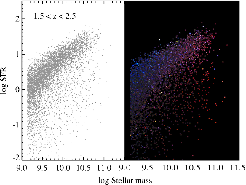
Another new test facilitated by the MRObs is comparison of the structural properties of galaxies in the semi-analytic model to those in real observations. In Fig. 22 we show a stellar mass versus SFR diagram for galaxies between and selected from one of our mock lightcone catalogs. In the panel on the right, we show postage stamps indicating the appearance of these galaxies in our simulated HST data (the image stamps are drawn from a mock colour-composite image based on the HST/ERS survey). These mock data can be used to measure galaxy structural properties (e.g., Sersic index, bulge-to-disk ratio, inclination), sizes and colours in exactly the same way as typically performed on real data only. By comparing measurements made based on the mock images with the exact physical quantities given by the semi-analytic model users could test how well such values can be recovered for a given data set, or for a given galaxy population. It also allows users to compare the structural properties of mock and real galaxies in a relatively unbiased way.
4.4 Selection of high redshift dropout galaxies
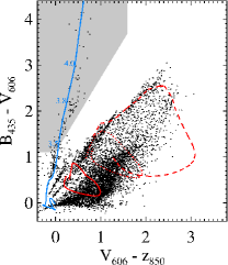
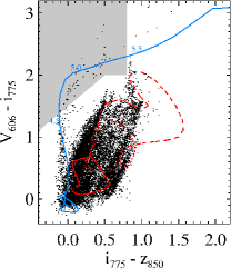
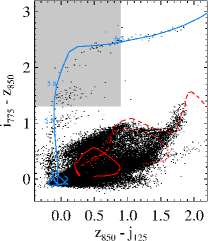
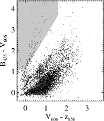
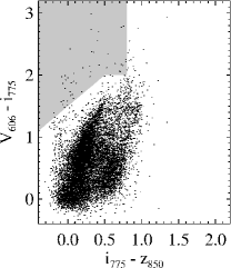
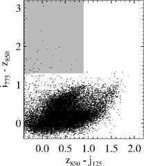
The last example we show here is the use of the MRObs in the selection of high redshift dropout galaxies from deep multi-wavelength imaging surveys and predictions thereof (e.g. Baugh et al., 1998; Blaizot et al., 2004; Guo & White, 2009; Overzier et al., 2009a). In Fig. 23 we show the colour-colour diagrams typically used to isolate galaxy samples at (-dropouts), (-dropouts), and (-dropouts). Objects at these high redshift suffer severe attenuation from the IGM in their spectra blue-ward of Ly (see §2.5). Consequently, these objects can be isolated from lower redshift galaxy population, as their Lyman break redshifts through a strategically chosen set of filters. Panels on the top show colour distributions for all objects found in one of our mock lightcones. The bottom panels show those objects that were detected in a mock survey based on the same lightcone. The limiting magnitudes used for the lightcone and for the extracted catalog were the same. This figure highlights some of the main differences between a pure semi-analytic model prediction (top panels) and what an observer actually sees (bottom panels). The colours of galaxies extracted from mock images are significantly scattered compared to their true (input) colours, making it harder to distinguish between low and high redshifts, or to derive their physical properties (e.g., redshift, mass, dust, star formation history, SFR) based on fitting their observed colours to a set of spectral synthesis models. It is straightforward to study and quantify such effects through the use of these kind of mock data. In the MRDB SQL queries can be performed to cross-match the SExtractor output catalogs to the lightcone or semi-analytic input catalogs, allowing one to investigate in detail the offsets between intrinsic and apparent properties, and to study which galaxies are included and excluded by certain observational selection criteria (e.g. colour-colour selections).
5 Public access to the MRObs data
5.1 MRObs database
As described above, the MRObs builds upon and extends the popular MRDB. Apart from the images, all the datasets produced by the MRObs and described in this paper are stored in a database that is accessible through the same interface as the MRDB itself777See http://gavo.mpa-garching.mpg.de/Millennium for a publicly accessible website giving access to the milli-Millennium database and information on how to gain access to the full database. and can be directly joined to the existing data sets. Here we give a summary description of the database and access methods, focusing on the new data products and how they are linked to the existing ones.
The MRDB is a relational database888This is not the place to describe relational databases in detail, there is sufficient information available online., where data sets are stored in tables (relations). A table generally stores objects of a particular type, with properties of these objects stored in columns. For example we have tables storing the the positions and velocities of particles from an N-body simulation, albeit a small one. We have tables with FOF groups and sub-halos as well as galaxies and many more. The web site giving access to these tables provides all information about the structure of the database.
An important feature of relational database design in general, and the MRDB in particular, is the possibility to manifest relations or links between objects in different tables. For example, a galaxy in the Munich semi-analytical model is always embedded in a subhalo. This relation is stored in the tables with galaxies as a column storing the (unique) identifier of the corresponding halo. The MRDB has a particularly rich set of such relations, especially where it deals with the relations between objects of the same type at different times (Lemson & Virgo Consortium, 2006).
Recent additions to the database were the results of the latest version of the Munich SAM from Guo et al. (2011) and pencil-beam and all sky light-cones derived from these in Henriques et al. (2012). The images produced by the MRObs from such light-cones do not lend themselves easily for storing in a database. However the SExtractor catalogues extracted from the images have been stored and we also have tables storing the different IGM absorption models described in §2.5. More information and examples on how to apply and cross-correlate the various MRDB and MRObs data sets are documented at the URL given below.
5.2 Data products of the MRObs
The MRObs delivers a number of entirely new data products to the community that are useful for independent analysis, or for serving as the starting point for new simulations. Here we will briefly describe the different types of new products.
5.2.1 Multi-wavelength lightcone catalogs with structural properties
The random field lightcones released as part of this paper are identical to the 24 multiwavelength lightcones measuring on the sky from Henriques et al. (2012), but with structural information added. The new structural information (sizes of the disk and bulge components, inclinations and position angles) is crucial for building the accurate galaxy models predicted by the MR simulations. These lightcones can be used, for example, to compare structural properties measured off the simulated images to the true input values. They can also be used as the starting point for users wishing to perform their own image simulations using realistic input catalogs based on the MR. In addition to the ‘random’ lightcones, we also release entirely new lightcones that specifically target galaxy clusters at a range of redshifts (see §2.4.2 and §4.2). All these lightcone catalogs are made available through the MRDB.
5.2.2 IGM tables
We provide tables that list the mean IGM attenuation as a function of redshift for a range of models (see §A). The IGM tables are applied to the lightcones to predict accurate colours and magnitudes of galaxies with redshift.
5.2.3 Object lists
Information from the structural light cones, the IGM tables, and a plate scale are combined to generate the input to the SkyMaker code that we use to create our synthetic ‘pre-observation’ images. These object lists may be used by other synthetic image simulators.
5.2.4 Pre-observation maps (‘perfect’ model images)
As described in §2.6, for each filter we build a so-called pre-observation or ‘perfect’ image that is based on the input object list. These images can be seen as a representation of the sky free of noise, PSF, or background. As such, they are easily convolved, rebinned, and scaled to match an arbitrary observation (typically a combination of a given telescope, camera, and exposure).
5.2.5 Simulated images
The ‘perfect’ images are turned into synthetic images that simulate real observational data. These images can be downloaded for further analysis. We also provide the PSF images that were used to convolve the perfect images to the instrument resolution, as well as documentation providing full details of how the images were produced.
5.2.6 SExtractor products
The simulated images are processed using SExtractor to produce the so-called segmentation maps identifying which image pixels correspond to which detected object, as well as the standard SExtractor output photometry catalogs. The SExtractor catalogs are made available through the MRDB where they can be searched or cross-matched with other data, such as lightcone catalogs, semi-analytic snapshots, dark matter halos, or density fields. The segmentation images are available for download.
5.3 Simulated surveys currently available in the MRObs
In its current deployment, the MRObs offers a number of data sets conveniently matched to some of the most popular extra-galactic surveys (e.g. the SDSS, CFHT-LS Wide and Deep, GOODS, UDF, GOODS/ERS, and CANDELS) for use by the community. Updates and future data releases will be announced through the MR web portal (URL given below), and in forthcoming publications.
5.4 The MRObs image browser
A special feature of the MRObs is that many of the data sets can also be accessed directly by means of our interactive MRObs image browser. This is an online tool that allows users to scan over and zoom into the synthetic images. These images are linked to the backend database (the MRDB) through a simple point-and-click function that allows retrieval of detailed information about the galaxies that are displayed. This is useful, for example, for familiarizing oneself with the relation between physical and observed properties of different types of galaxies or galaxies at different redshifts, for selecting interesting objects from the MR simulations for subsequent analysis, for comparing the quality expected for different types of data sets or telescopes, and for didactical and outreach purposes. Here we describe the main features of the MRObs browser in brief.
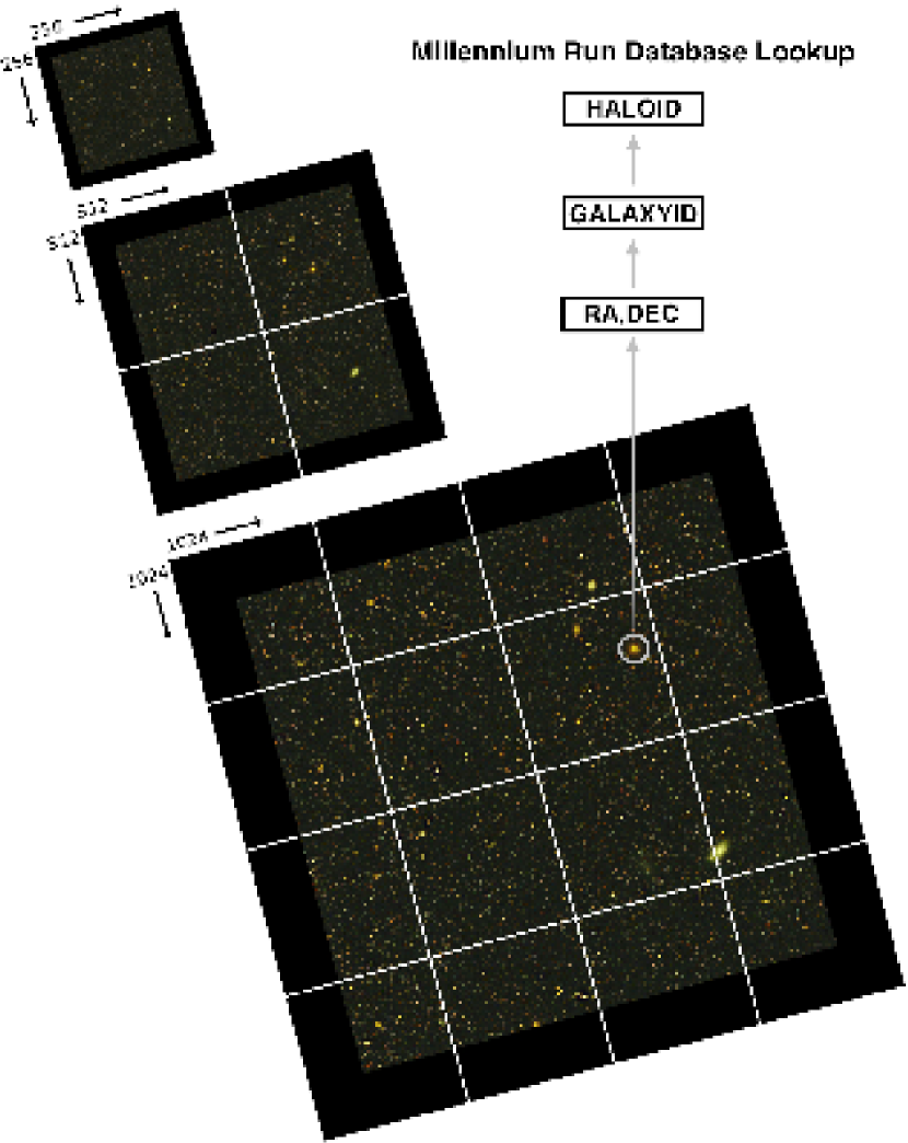
5.4.1 Deep zoom RGB image pyramids
The images produced by the MRObs are typically very large. For example, a simulated HST survey covering an area of at a (drizzled) pixel scale of already measures 20,00020,000 pixels (400 Megapixels), and in principle the MRObs could create much larger fields at much higher resolution than this. These images therefore do not fit on a standard computer screen. Using a technology similar to, e.g., Google Maps, the MRObs browser allows users to efficiently pan around and zoom in such large, high resolution images. We here describe in some detail how we have implemented this truly virtual telescope.
First the simulated, multi-wavelength filter images are combined into false-colour RGB composites. We use the publicly available code STIFF999http://astromatic.net/software/stiff that handles the conversion from arbitrarily large scientific FITS input images to standard TIFF format output images (Bertin, 2012). STIFF automatically (or manually) applies contrast and brightness adjustments, colour balance and saturation, and gamma corrections producing colour images that are highly informative of the level of detail present in the mono-chromatic input fits images. When we have multiple bands available for any of the three RGB channels (for example when making colour composites of data sets based on more than three filters), we reduce the number of input images to three by creating variance-weighted averages and use those as the input for each channel.
From this high-resolution image we then create a so-called ‘image pyramid’ consisting of representations of this high resolution image at ever decreasing resolution. The method is illustrated in Fig. 24. The top of the pyramid (level 0) consists of a single pixels low resolution image that is a heavily rebinned version of the original or full-resolution pixels image. The next level contains image tiles each of times higher resolution compared to the previous level. At the th level (corresponding to the base of the pyramid), there will be tiles each representing only a small portion of the original image but now at its highest resolution.
The browser software101010We use the Deep Zoom technology developed by Seadragon/Microsoft embedded in custom written java script libraries. uses this data format to download only those tiles that at the current zoom level are required to show the image. This significantly reduces the download time and creates a smooth transition between the different levels or different regions of the image when viewed in a web browser. For example, if we adopt a factor of scalings between levels, tiles of pixels, and an original image of pixels, the last level (level 7) will consist of tiles of pixels. This means that only about 0.1% of data needs to be downloaded at any time to display a particular region at its fullest resolution on a resolution display.
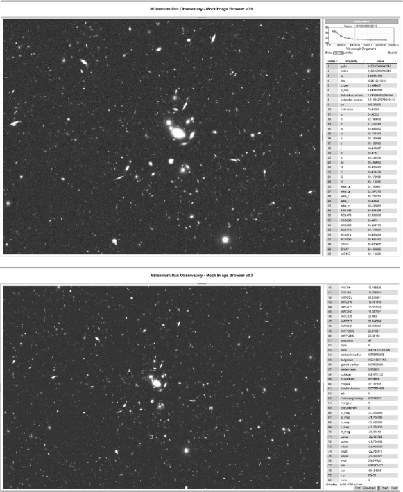
5.4.2 User interface of the MRObs browser
The MRObs Browser offers the user the choice of a large number of image pyramids, based on sets of different mock images, for a variety of virtual telescopes and with different wavelength bands. Each mock image is derived from a light cone stored in the MRDB, and the MRObs Browser allows interactive querying of these cones.
Screen-shots of an HST simulation viewed through he MRObs Browser are shown in Fig. 25. Clicking the image leads to an SQL query being submitted to the database that searches for the nearest galaxy to the selected (virtual) sky position, up to a maximum radius (currently 1″). If a galaxy is found a large amount of information is retrieved and displayed in a table on the screen next to the image, as shown on the right hand side of the screenshots in Fig. 25. The selected galaxy is indicated on the image with a little white square (top panel). The table includes information of the galaxy on the light cone, such as redshift, apparent sizes and luminosities in up to 40 bands. The observed-frame SED is shown in graphical form above the table. It also includes, through the linking of the light-cone galaxy to the underlying semi-analytical galaxy catalogues, information about physical parameters such as stellar mass, gas mass, metallicities and rest frame magnitudes in the SDSS bands. The information also includes details about the original dark-matter subhalo and friends-of-friends group the galaxy belongs to. The latter information can in its turn be used to search for all other galaxies in the image that belong to the same FOF group as the selected galaxy. In the bottom panel, the positions of all galaxies that were retrieved are indicated on the screen. The structure turns out to be a galaxy group at .
The query capabilities of the MRObs Browser will be extended over time and will be tied to the plain SQL query capabilities of the MRDB.
6 Future developments
Future refinements of the modeling recipes in the MRObs currently in preparation include the calculation of extinctions based on the physically motivated inclinations of galaxies (§2.4.3), as well as the inclusion of strong gravitational lensing based on the distribution of dark matter halos along each lightcone. Although the current simulations span the observed far-UV to the observed near-IR, improvements in the dust-modeling should eventually allow us to construct images out to far-infrared and sub-mm wavelengths. Future simulated surveys will be made available through the MRObs web portal. Ultimately, fully interactive, online versions of the SAM, the lightcone generator, and the telescope simulator will allow users of the MRObs even greater flexibility in performing the simulations that best suit their needs.
7 Summary
In order to make predictions in the observational plane and to allow unbiased comparisons between semi-analytic models and real data, we have developed the Millennium Run Observatory (MRObs), a new virtual telescope facility that can be used to simulate realistic observational data based on the semi-analytic model galaxy catalogues associated with the dark matter MR simulations. The MRObs allows one to produce scientific image data sets in .fits format. These artificial data can be analyzed using the standard tools routinely used for analyzing real observations, allowing a relatively unbiased comparison between SAMs and real data. This contrasts with previous studies that compare highly idealized SAM predictions to observational data. The new technique will help – but is by no means limited – to:
-
•
Extend the MR simulations project approach by producing data products directly corresponding to observations, namely synthetic images and extracted source catalogs
-
•
Aid theorists in testing analytical models against observations
-
•
Aid observers in making detailed predictions for observations and better analyses of observational data
-
•
Allow the community to subject the models to new kinds of tests
-
•
Allow detailed comparisons with synthetic observations produced by other groups performing cosmological simulations
-
•
Allow calibration of observational analysis methods by making available synthetic data for which the entire underlying physical ‘reality’ is known.
-
•
Extend the realism with which semi-analytic models can address questions such as what is the probability that a galaxy will be detected within a particular observational data set?
-
•
Allow one to explore the uniqueness of certain physical models that are based on the analysis of astronomical images, as different models or different parameter sets may produce indistinguishable synthetic observations.
-
•
Provide a framework for future virtual theoretical observatories
One of the great advantages provided by our extended modeling approach is that for the synthetic observations produced by the MRObs, the physical properties (e.g., dark matter halo mass, SFR, stellar mass, size, redshift) and photometric properties (e.g., magnitudes and colours) of every galaxy are precisely known, in contrast to real observations where one does not know the exact or ‘true’ answer. This makes the MRObs an ideal facility for calibrating many of the measurement and analysis techniques that are applied to real observations. The MRObs will allow observers and theorists to approach a problem from different directions with freedom in deciding where to meet.
We have introduced a modified lightcone technique that allows us to create lightcones aimed at selected objects or regions placed at any desired position or orientation. The new technique is useful for extending the range of questions that can be asked of the MRObs, such as what would be the appearance of a particular galaxy cluster at ? What does this same cluster look like at or at ? How is the interpretation of observations of such structures affected by viewing angle or chance superpositions? Special cones centred on clusters at a range of redshifts have been added to the MRDB for studies of cluster evolution.
Attenuation by the IGM is applied to the lightcones statistically using the baseline model from Madau (1995), as well as two more recent implementations based on Monte Carlo modeling of the IGM by Harrison et al. (2011). Our IGM attenuation tables have also been added to the MRDB such that they can be used to apply ‘on the fly’ IGM absorption corrections to lightcones (see the MRObs URL for a tutorial on how to apply the IGM absorption corrections to the lightcones from Henriques et al. (2012) also available in the MRDB). This is essential for making comparisons with high redshift observations.
In order to allow the community to use our predictions as the basis for other mock observation experiments, we provide not only our final image products, but also the intermediate steps such as the input object lists and the pre-observation model images.
In order to introduce the communities of theoretically and
observationally inclined researchers to the ‘added value’ of the
MRObs modeling approach, we have provided the following four example
user cases:
(1) We compared the galaxy number counts in the CANDELS/UDS survey
with the predicted counts taken directly from the semi-analytic
lightcone and with the counts extracted from synthetic CANDELS images
(Fig. 18 and §4.1). Interestingly,
the counts recovered from the synthetic images are lower than those
predicted by the lightcone that was used to construct the synthetic
observation, suggesting that the discrepancy between semi-analytic
model predictions and observations may be smaller than previously
claimed. The implications of this will be detailed in a followup paper
(Overzier et al., in prep.).
(2) We simulated images of galaxy clusters seen with SDSS and HST at a
range of redshifts (Figs. 19–21 and
§4.2). We also showed synthetic images of the
same galaxy cluster at from three different directions,
illustrating that orientation effects can be important when
interpreting the visual appearance of large-scale structure at high
redshift.
(3) We showed how the MRObs allows one to study the detailed
structural properties of semi-analytic galaxies in synthetic images
(Fig. 22 and §4.3). In these synthetic images
one can measure colours, sizes, bulge-to-disk ratios and profile shapes
using standard observational techniques. The outcome of these
measurements can then be compared to the intrinsic values provided by
the MRObs, or to measurements performed on real galaxies.
(4) We showed how the MRObs images can be used to search for high
redshift dropout galaxies in a manner that is directly analogous to
that used for real high redshift doprout searches
(Fig. 23 and §4.4). This enables a
much more realistic comparison with the data, and allows us to assess
how well we are able to derive the intrinsic physical properties from
the observations.
Extending the successful open-access approach of the MR project, we make available new data products for use by the community. As part of our first data release, we have produced simulated data that emulates a number of key surveys, including SDSS, CFHT-LS (Wide and Deep), GOODS, HUDF, GOODS/ERS, and CANDELS (UDS, COSMOS and GOODS-S). The data sets are modeled using two different cosmologies (WMAP1 and WMAP7), two spectral synthesis models (BC03 and M05), and three IGM absorption models (MADAU, MEIKSIN, and INOUE-IWATA). In specific cases, we provide synthetic images that have the exact same geometric and identical noise properties as the reference survey. The MRObs data can furthermore be explored using an online image browser that allows users to interactively explore the available mock observations. The browser graphically links objects (galaxies) in the synthetic images to various types of information available in catalogs in the MRDB. For each synthetic galaxy, this information includes the physical properties of their dark matter halos, the intrinsic properties of the galaxy itself, the absolute and apparent photometric properties, and the observed properties recovered from the synthetic images using SExtractor.
The public data and the MRObs browser can be accessed at the following URL:
http://galformod.mpa-garching.mpg.de/mrobs/
In conclusion, the MRObs allows us to study our simulated universes through the eyes of our telescopes. We hope that the methods and data presented in this paper will encourage others to take advantage of the new opportunities offered by this approach.
Acknowledgments
We thank Rychard Bouwens, Yi-Kuan Chiang, Marijn Franx, Guinevere Kauffmann, Jaewon Kim, Ben Metcalfe, and Masami Ouchi for helpful discussions. We thank Chris Harrison for making his code IGMTransmission publicly available and for his clarifications. We thank Russell Ryan, Seth Cohen, Rogier Windhorst and other members of the GOODS ERS team for discussions and supplying us with their empirical PSFs. We thank Daniel Harsono for providing the HST/ACS images of Cl0024 used in Fig. 20. We thank Matthias Egger for his excellent technical support. The Millennium Simulation databases used in this paper and the web application providing online access to them were constructed as part of the activities of the German Astrophysical Virtual Observatory. This work was supported by Advanced Grant 246797 ‘GALFORMOD’ from the European Research Council. The authors acknowledge the Texas Advanced Computing Center (TACC) at The University of Texas at Austin for providing the 307 Mpixel tiled-display system (Stallion) and the 12.4 Mpixel multi-touch display (Lasso) visualization resources that have contributed to developing the methods and results reported within this paper. We thank Ben Urick and Brandt Westing of TACC for their time and expert support.
| FILTERID | Description | FILTERID | Description |
|---|---|---|---|
| U | Johnson | ACS435 | HST/ACS-WFC F435W |
| B | Johnson | ACS475 | HST/ACS-WFC F475W |
| V | Johnson | ACS606 | HST/ACS-WFC F606W |
| Rc | Cousins | ACS625 | HST/ACS-WFC F625W |
| Ic | Cousins | ACS775 | HST/ACS-WFC F775W |
| Z | UKIDDS | ACS814 | HST/ACS-WFC F814W |
| Y | UKIDDS | ACS850 | HST/ACS-WFC F850LP |
| J | UKIDDS | GFUV | GALEX FUV |
| H | UKIDDS | GNUV | GALEX NUV |
| K | Johnson | NIC110 | HST/NICMOS F110W |
| Ks | UKIDDS | NIC160 | HST/NICMOS F160W |
| i1 | Spitzer/IRAC channel 1 | VIMOSU | VLT/VIMOS |
| i2 | Spitzer/IRAC channel 2 | WFC105 | HST/WFC3-IR F105W |
| i3 | Spitzer/IRAC channel 3 | WFC125 | HST/WFC3-IR F125W |
| i4 | Spitzer/IRAC channel 4 | WFC160 | HST/WFC3-IR F160W |
| SDSS_u | SDSS | WFC225 | HST/WFC3-UVIS F225W |
| SDSS_g | SDSS | WFC275 | HST/WFC3-UVIS F275W |
| SDSS_r | SDSS | WFC336 | HST/WFC3-UVIS F336W |
| SDSS_i | SDSS | WFPC300 | HST/WFPC2 F300W |
| SDSS_z | SDSS | WFPC450 | HST/WFPC2 F450W |
References
- Angulo & White (2010) Angulo, R. E., & White, S. D. M. 2010, MNRAS, 405, 143
- Angulo et al. (2012) Angulo, R. E., Springel, V., White, S. D. M., et al. 2012, arXiv:1203.3216
- Baugh et al. (1998) Baugh, C. M., Cole, S., Frenk, C. S., & Lacey, C. G. 1998, ApJ, 498, 504
- Baugh et al. (2005) Baugh, C. M., Lacey, C. G., Frenk, C. S., et al. 2005, MNRAS, 356, 1191
- Benson et al. (2003) Benson, A. J., Bower, R. G., Frenk, C. S., et al. 2003, ApJ, 599, 38
- Bertin & Arnouts (1996) Bertin, E., & Arnouts, S. 1996, A&AS, 117, 393
- Bertin (2009) Bertin, E. 2009, Memorie della Societá Astronomica Italiana, 80, 422
- Bertin (2012) Bertin, E. 2012, in Proceedings of ADASS XXI P.Ballester and D.Egret editors, in press
- Bertone et al. (2007) Bertone, S., DeLucia, G., & Thomas, P. A., 2007, MNRAS, 379, 1143
- Bershady et al. (1999) Bershady, M. A., Charlton, J. C., & Geoffroy, J. M. 1999, ApJ, 518, 103
- Blaizot et al. (2004) Blaizot, J., Guiderdoni, B., Devriendt, J. E. G., et al. 2004, MNRAS, 352, 571
- Blaizot et al. (2005) Blaizot, J., Wadadekar, Y., Guiderdoni, B., et al. 2005, MNRAS, 360, 159
- Bouché et al. (2010) Bouché, N., Dekel, A., Genzel, R., et al. 2010, ApJ, 718, 1001
- Bouwens et al. (1999) Bouwens, R., Cayón, L., & Silk, J. 1999, ApJ, 516, 77
- Bouwens et al. (2003) Bouwens, R. J., Illingworth, G. D., Rosati, P., et al. 2003, ApJ, 595, 589
- Bouwens et al. (2006) Bouwens, R. J., Illingworth, G. D., & Magee, D. K. 2006, Astronomical Data Analysis Software and Systems XV, 351, 145
- Bower et al. (2006) Bower, R. G., Benson, A. J., Malbon, R., et al. 2006, MNRAS, 370, 645
- Boylan-Kolchin et al. (2009) Boylan-Kolchin, M., Springel, V., White, S. D. M., Jenkins, A., & Lemson, G. 2009, MNRAS, 398, 1150
- Bruzual & Charlot (2003) Bruzual, G., & Charlot, S. 2003, MNRAS, 344, 1000
- Bruzual (2007) Bruzual, G. 2007, From Stars to Galaxies: Building the Pieces to Build Up the Universe, 374, 303
- Cardelli et al. (1989) Cardelli, J. A., Clayton, G. C., & Mathis, J. S. 1989, ApJ, 345, 245
- Carlson & White (2010) Carlson, J., & White, M. 2010, ApJS, 190, 311
- Casertano et al. (2000) Casertano, S., de Mello, D., Dickinson, M., et al. 2000, AJ, 120, 2747
- Cattaneo et al. (2005) Cattaneo, A., Blaizot, J., Devriendt, J., & Guiderdoni, B. 2005, MNRAS, 364, 407
- Cattaneo et al. (2006) Cattaneo, A., Dekel, A., Devriendt, J., Guiderdoni, B., & Blaizot, J. 2006, MNRAS, 370, 1651
- Ceverino et al. (2010) Ceverino, D., Dekel, A., & Bournaud, F. 2010, MNRAS, 404, 2151
- Chilingarian et al. (2010) Chilingarian, I. V., Di Matteo, P., Combes, F., Melchior, A.-L., & Semelin, B. 2010, A&A, 518, A61
- Cirasuolo et al. (2010) Cirasuolo, M., McLure, R. J., Dunlop, J. S., et al. 2010, MNRAS, 401, 1166
- Cole et al. (1994) Cole, S., Aragon-Salamanca, A., Frenk, C. S., Navarro, J. F., & Zepf, S. E. 1994, MNRAS, 271, 781
- Cole et al. (1998) Cole, S., Hatton, S., Weinberg, D. H., & Frenk, C. S. 1998, MNRAS, 300, 945
- Cole et al. (2000) Cole, S., Lacey, C. G., Baugh, C. M., & Frenk, C. S., 2000, MNRAS, 319, 168
- Connolly et al. (2010) Connolly, A. J., Peterson, J., Jernigan, J. G., et al. 2010, SPIE, 7738,
- Conroy et al. (2009) Conroy, C., Gunn, J. E., & White, M. 2009, ApJ, 699, 486
- Croton et al. (2006) Croton, D. J., Springel, V., White, S. D. M., et al. 2006, MNRAS, 365, 11
- Cucciati et al. (2012) Cucciati, O., De Lucia, G., Zucca, E., et al. 2012, arXiv:1205.1517
- De Lucia & Blaizot (2007) De Lucia, G., & Blaizot, J. 2007, MNRAS, 375, 2
- Davis et al. (1982) Davis, M., Huchra, J., Latham, D. W., & Tonry, J. 1982, ApJ, 253, 423
- Davis et al. (1985) Davis, M., Efstathiou, G., Frenk, C. S., & White, S. D. M. 1985, ApJ, 292, 371
- Dekel et al. (2009) Dekel, A., Sari, R., & Ceverino, D. 2009, ApJ, 703, 785
- Diaferio et al. (1999) Diaferio, A., Kauffmann, G., Colberg, J. M., & White, S. D. M. 1999, MNRAS, 307, 537
- Dobke et al. (2010) Dobke, B. M., Johnston, D. E., Massey, R., et al. 2010, PASP, 122, 947
- Dutton et al. (2010) Dutton, A. A., van den Bosch, F. C., & Dekel, A. 2010, MNRAS, 405, 1690
- Eminian et al. (2008) Eminian, C., Kauffmann, G., Charlot, S., et al. 2008, MNRAS, 384, 930
- Erben et al. (2001) Erben, T., Van Waerbeke, L., Bertin, E., Mellier, Y., & Schneider, P. 2001, A&A, 366, 717
- Finkelstein et al. (2010) Finkelstein, S. L., Papovich, C., Giavalisco, M., et al. 2010, ApJ, 719, 1250
- Finlator et al. (2011) Finlator, K., Oppenheimer, B. D., & Davé, R. 2011, MNRAS, 410, 1703
- Fioc & Rocca-Volmerange (1997) Fioc, M., & Rocca-Volmerange, B. 1997, A&A, 326, 950
- Forero-Romero et al. (2007) Forero-Romero, J. E., Blaizot, J., Devriendt, J., van Waerbeke, L., & Guiderdoni, B. 2007, MNRAS, 379, 1507
- Fruchter et al. (2009) Fruchter, A., Sosey, M., et al. 2009, ‘The MultiDrizzle Handbook’, version 3.0, (Baltimore, STScI)
- Gibson et al. (2011) Gibson, R. R., Ahmad, Z., Bankert, J., et al. 2011, Astronomical Data Analysis Software and Systems XX, 442, 329
- Girardi et al. (2005) Girardi, L., Groenewegen, M. A. T., Hatziminaoglou, E., & da Costa, L. 2005, A&A, 436, 895
- González et al. (2011) González, V., Labbé, I., Bouwens, R. J., et al. 2011, ApJL, 735, L34
- Grogin et al. (2011) Grogin, N. A., Kocevski, D. D., Faber, S. M., et al. 2011, ApJS, 197, 35
- Guo & White (2009) Guo, Q., & White, S. D. M. 2009, MNRAS, 396, 39
- Guo et al. (2011) Guo, Q., White, S., Boylan-Kolchin, M., et al. 2011, MNRAS, 413, 101
- Guo et al. (2012) Guo, Q., White, S., Angulo, R. E., et al. 2012, MNRAS, submitted (arXiv:1206.0052)
- Hamana et al. (2001) Hamana, T., Colombi, S., & Suto, Y. 2001, A&A, 367, 18
- Harrison et al. (2011) Harrison, C. M., Meiksin, A., & Stock, D. 2011, arXiv:1105.6208
- Harsono & De Propris (2009) Harsono, D., & De Propris, R. 2009, AJ, 137, 3091
- Hatton et al. (2003) Hatton, S., Devriendt, J. E. G., Ninin, S., et al. 2003, MNRAS, 343, 75
- Henriques et al. (2011) Henriques, B., Maraston, C., Monaco, P., et al. 2011, MNRAS, 415, 3571
- Henriques et al. (2012) Henriques, B. M. B., White, S. D. M., Lemson, G., et al. 2012, MNRAS, 421, 2904
- Heymans et al. (2006) Heymans, C., Van Waerbeke, L., Bacon, D., et al. 2006, MNRAS, 368, 1323
- Inoue & Iwata (2008) Inoue, A. K., & Iwata, I. 2008, MNRAS, 387, 1681
- Jee et al. (2007) Jee, M. J., Ford, H. C., Illingworth, G. D., et al. 2007, ApJ, 661, 728
- Jenkins et al. (1998) Jenkins, A., Frenk, C. S., Pearce, F. R., et al. 1998, ApJ, 499, 20
- Jonsson et al. (2010) Jonsson, P., Groves, B. A., & Cox, T. J. 2010, MNRAS, 403, 17
- Jonsson et al. (2006) Jonsson, P., Cox, T. J., Primack, J. R., & Somerville, R. S. 2006, ApJ, 637, 255
- Kang et al. (2005) Kang, X., Jing, Y. P., Mo, H. J., & Börner, G., 2005, ApJ, 631, 21
- Kauffmann & White (1993) Kauffmann, G., & White, S. D. M. 1993, MNRAS, 261, 921
- Kauffmann et al. (1993) Kauffmann, G., White, S. D. M., & Guiderdoni, B. 1993, MNRAS, 264, 201
- Kauffmann et al. (1999) Kauffmann, G., Colberg, J. M., Diaferio, A., & Wite, S. D. M. 1999, MNRAS, 303, 188
- Kauffmann & Haehnelt (2000) Kauffmann, G., & Haehnelt, M. 2000, MNRAS, 311, 576
- Kereš et al. (2009) Kereš, D., Katz, N., Fardal, M., Davé, R., & Weinberg, D. H. 2009, MNRAS, 395, 160
- Kitzbichler & White (2006) Kitzbichler, M. G., & White, S. D. M. 2006, MNRAS, 366, 858
- Kitzbichler & White (2007) Kitzbichler, M. G., & White, S. D. M. 2007, MNRAS, 376, 2
- Klypin et al. (2011) Klypin, A. A., Trujillo-Gomez, S., & Primack, J. 2011, ApJ, 740, 102
- Koekemoer et al. (2003) Koekemoer, A. M., Fruchter, A. S., Hook, R. N., & Hack, W. 2003, The 2002 HST Calibration Workshop : Hubble after the Installation of the ACS and the NICMOS Cooling System, Proceedings of a Workshop held at the Space Telescope Science Institute, Baltimore, Maryland, October 17 and 18, 2002. Edited by Santiago Arribas, Anton Koekemoer, and Brad Whitmore. Baltimore, MD: Space Telescope Science Institute, 2003., p.337, 337
- Koekemoer et al. (2011) Koekemoer, A. M., Faber, S. M., Ferguson, H. C., et al. 2011, ApJS, 197, 36
- Kriek et al. (2006) Kriek, M., van Dokkum, P. G., Franx, M., et al. 2006, ApJL, 649, L71
- Kriek et al. (2010) Kriek, M., Labbé, I., Conroy, C., et al. 2010, ApJL, 722, L64
- Lacey & Cole (1994) Lacey, C. & Cole, S. 1994, MNRAS, 271, 676
- Lee et al. (2010) Lee, S.-K., Ferguson, H. C., Somerville, R. S., Wiklind, T., & Giavalisco, M. 2010, ApJ, 725, 1644
- Leitherer & Heckman (1995) Leitherer, C., & Heckman, T. M. 1995, ApJS, 96, 9
- Lemson & Virgo Consortium (2006) Lemson, G., & Virgo Consortium, 2006, arXiv:astro-ph/0608019
- Lotz et al. (2008) Lotz, J. M., Jonsson, P., Cox, T. J., & Primack, J. R. 2008, MNRAS, 391, 1137
- Lotz et al. (2010) Lotz, J. M., Jonsson, P., Cox, T. J., & Primack, J. R. 2010, MNRAS, 404, 575
- Madau (1995) Madau, P. 1995, ApJ, 441, 18
- Maraston (1998) Maraston, C. 1998, MNRAS, 300, 872
- Maraston (2005) Maraston, C. 2005, MNRAS, 362, 799
- Maraston et al. (2006) Maraston, C., Daddi, E., Renzini, A., et al. 2006, ApJ, 652, 85
- Maraston et al. (2010) Maraston, C., Pforr, J., Renzini, A., et al. 2010, MNRAS, 407, 830
- Marchesini et al. (2010) Marchesini, D., Whitaker, K. E., Brammer, G., et al. 2010, ApJ, 725, 1277
- Marinoni et al. (2005) Marinoni, C., Le Fèvre, O., Meneux, B., et al. 2005, A&A, 442, 801
- Meiksin (2006) Meiksin, A. 2006, MNRAS, 365, 807
- Mo & White (1996) Mo, H. J., & White, S. D. M. 1996, MNRAS, 282, 347
- Monaco et al. (2007) Monaco, P., Fontanot, F., & Taffoni, G. 2007, MNRAS, 375, 1189
- Neistein & Dekel (2008) Neistein, E., & Dekel, A. 2008, MNRAS, 383, 615
- Neistein & Weinmann (2010) Neistein, E., & Weinmann, S. M. 2010, MNRAS, 405, 2717
- Ouchi et al. (2005) Ouchi, M., Hamana, T., Shimasaku, K., et al. 2005, ApJL, 635, L117
- Overzier et al. (2006) Overzier, R. A., Bouwens, R. J., Illingworth, G. D., & Franx, M. 2006, ApJL, 648, L5
- Overzier et al. (2009a) Overzier, R. A., Guo, Q., Kauffmann, G., et al. 2009a, MNRAS, 394, 577
- Overzier et al. (2009b) Overzier, R. A., Shu, X., Zheng, W., et al. 2009b, ApJ, 704, 548
- Papovich et al. (2011) Papovich, C., Finkelstein, S. L., Ferguson, H. C., Lotz, J. M., & Giavalisco, M. 2011, MNRAS, 412, 1123
- Pforr et al. (2012) Pforr, J., Maraston, C., & Tonini, C. 2012, MNRAS, 422, 3285
- Pollo et al. (2006) Pollo, A., Guzzo, L., Le Fèvre, O., et al. 2006, A&A, 451, 409
- Prada et al. (2012) Prada, F., Klypin, A. A., Cuesta, A. J., Betancort-Rijo, J. E., & Primack, J. 2012, MNRAS, 423, 3018
- Press & Schechter (1974) Press, W. H., & Schechter, P. 1974, ApJ, 187, 425
- Robertson & Bullock (2008) Robertson, B. E., & Bullock, J. S. 2008, ApJL, 685, L27
- Ruiz et al. (2011) Ruiz, A. N., Padilla, N. D., Domínguez, M. J., & Cora, S. A. 2011, MNRAS, 1600
- Sheth et al. (2001) Sheth, R. K., Mo, H. J., & Tormen, G. 2001, MNRAS, 323, 1
- Somerville & Primack (1999) Somerville, R. S., & Primack, J. R. 1999, MNRAS, 310, 1087
- Somerville & Kolatt (1999) Somerville, R. S., & Kolatt, T. S. 1999, MNRAS, 305, 1
- Somerville et al. (2001) Somerville, R. S., Primack, J. R., & Faber, S. M. 2001, MNRAS, 320, 504
- Somerville et al. (2008) Somerville, R. S., Hopkins, P. F., Cox, T. J., Robertson, B. E., & Hernquist, L. 2008, MNRAS, 391, 481
- Somerville et al. (2012) Somerville, R. S., Gilmore, R. C., Primack, J. R., & Domínguez, A. 2012, MNRAS, 423, 1992
- Sousbie et al. (2008) Sousbie, T., Courtois, H., Bryan, G., & Devriendt, J. 2008, ApJ, 678, 569
- Spergel et al. (2003) Spergel, D. N., Verde, L., Peiris, H. V., et al. 2003, ApJS, 148, 175
- Springel et al. (2001) Springel, V., White, S. D. M., Tormen, G., & Kauffmann, G. 2001, MNRAS, 328, 726
- Springel et al. (2005) Springel, V., White, S. D. M., Jenkins, A., et al. 2005, Nature, 435, 629
- Teyssier et al. (2009) Teyssier, R., Pires, S., Prunet, S., et al. 2009, A&A, 497, 335
- Tinsley (1973) Tinsley, B. M. 1973, ApJ, 186, 35
- Tinsley (1980) Tinsley, B. M. 1980, FCPh, 5, 287
- Tonini et al. (2009) Tonini, C., Maraston, C., Devriendt, J., Thomas, D., & Silk, J. 2009, MNRAS, 396, L36
- Tonini et al. (2010) Tonini, C., Maraston, C., Thomas, D., Devriendt, J., & Silk, J. 2010, MNRAS, 403, 1749
- de la Torre et al. (2011) de la Torre, S., Meneux, B., De Lucia, G., et al. 2011, A&A, 525, A125
- Vázquez & Leitherer (2005) Vázquez, G. A., & Leitherer, C. 2005, ApJ, 621, 695
- White & Frenk (1991) White, S. D. M., & Frenk, C. S. 1991, ApJ, 379, 52
- Windhorst et al. (2011) Windhorst, R. A., Cohen, S. H., Hathi, N. P., et al. 2011, ApJS, 193, 27
- Wuyts et al. (2009) Wuyts, S., Franx, M., Cox, T. J., et al. 2009, ApJ, 700, 799
Appendix A Intergalactic medium corrections
The MEIKSIN and INOUE-IWATA models (Meiksin, 2006; Inoue & Iwata, 2008) discussed in §2.5 are both based on a Monte Carlo approach that distributes LLSs chosen from a redshift distribution and an optical depth distribution (both constrained by observations), and averages over the IGM transmission measured along a large number of random lines of sight. The IGM effective optical depth at observed wavelength is taken to be the sum of the Lyman continuum (LC) optical depth due to LLSs, the optically thin IGM, and the Ly forest as follows:
| (7) |
The optical depth due to photoelectric absorption by LLSs along the line of sight to a source at redshift is given by
with , and the number of absorbers per unit redshift and optical depth. In the MEIKSIN model the LLSs are randomly drawn from the distributions
| (9) | |||||
| (10) |
while INOUE-IWATA assumes
| (14) |
| (15) |
with , , , , , and . The mean IGM transmission due to the LLSs typically stabilizes after averaging over 10,000 random lines of sight. Following Meiksin (2006) and Harrison et al. (2011), both models include a static contribution from the diffuse or optically thin IGM and the Ly forest:
| (16) | |||||
| (17) |
with and the Lyman transitions up to are included.
For completeness, we also give the MADAU modeling approximation (Madau, 1995):
| (18) | |||||
with for ) Å, , , , and is the redshift of the source. Eq. LABEL:eq:madau is the approximation given for Eq. 16 in Madau (1995, see footnote 3 in that paper).