Basic Singular Spectrum Analysis and
Forecasting with R

Abstract

Singular Spectrum Analysis (SSA) is a powerful tool of analysis and forecasting of time series. In this paper we describe the main features of the Rssa package, which efficiently implements the SSA algorithms and methodology in R. Analysis, forecasting and parameter estimation are demonstrated using case studies. These studies are supplemented with accompanying codes in R.

1 Introduction

Singular Spectrum Analysis (SSA) is a well-developed methodology of time series analysis and forecasting which comprises many different but inter-linked methods. There are several books devoted to SSA (Elsner and Tsonis, 1996; Golyandina et al., 2001; Golyandina and Zhigljavsky, 2013) as well as many papers related to the theory of SSA and especially to various applications of SSA (see Golyandina and Zhigljavsky (2013) for references). The scope of applications of SSA is very wide, from non-parametric time series decomposition and filtration to parameter estimation and forecasting.

One of the differences between SSA and the methods of traditional time series analysis is the fact that SSA and SSA-related methods can be applied to quite different and not conventional for classical time series analysis problems such as exploratory analysis for data-mining and parameter estimation in signal processing, among others. In this paper we mostly concentrate on exploratory analysis by SSA; however, the tools for model construction and parameter estimation are described too. Despite no model is assumed before the SSA method is applied, the so-called subspace-based model is constructed adaptively; the corresponding class of time series includes time series governed by linear recurrence relations in presence of noise. Linear recurrence relations are associated with autoregressive (AR) models. However, note that the AR model of stationary processes is very different from the model of noisy time series governed by LRR, which is associated with the model of deterministic signal (generally, non-stationary) corrupted by noise. Therefore these models are formally not comparable. For real-world time series whose models are unknown, AR and SSA can be numerically compared, see e.g. Hassani et al. (2009). The essential difference between SSA and the majority of methods that analyze time series with a trend and/or periodicities lies in the fact that SSA does not require an a-priori model for trend as well as the a-priori knowledge of number of periodicities and period values. Also, periodicities can be modulated by different ways and therefore the type of model, additive or multiplicative, is not necessary to be hold and taken into consideration.

Any method needs effective, comfortable and accessible implementation. There are many implementations of SSA. They differ by potential application areas, implemented methods, interactive on non-interactive form, free or commercial use, computer system (Windows, Unix, Mac), level of reliability and support. The most known supported software packages implementing SSA are the following:

1. http://gistatgroup.com:
   general-purpose interactive ‘Caterpillar’-SSA software (Windows) following the methodology described in Golyandina et al. (2001); Golyandina and Zhigljavsky (2013);

2. http://www.atmos.ucla.edu/tcd/ssa:
   oriented mainly on climatic applications SSA-MTM Toolkit for spectral analysis (Ghil et al., 2002) (Unix) and its commercial extension kSpectra Toolkit (Mac), interactive;

3. The commercial statistical software, SAS, includes SSA to its econometric extension SAS/ETS®Software based on methodology of Golyandina et al. (2001).

4. http://cran.r-project.org/web/packages/Rssa:
   R package Rssa (Korobeynikov, 2010), a novel implementation of the main SSA procedures for major platforms, extensively developed.

We consider the Rssa package as an efficient implementation of the main SSA algorithms. This package also contains many visual tools which are useful for making proper choice of SSA parameters and examination of the results. At present, Rssa is the only SSA implementation available from CRAN and almost certainly the fastest implementation of the SSA. Another important feature of the package is its very close relation to the SSA methodology thoroughly described in Golyandina et al. (2001); Golyandina and Zhigljavsky (2013). As a result of this, the use of the package is well theoretically and methodologically supported. Note, however, that the package has been created only recently (within the last 2 years) and therefore cannot be perfect. We are aware about the ways of its further development and currently working on this development.

The aim of this paper is to show how the methodology of the SSA analysis, forecasting and parameter estimation can be implemented with the help of the package Rssa. Certainly, it is hard to study a method using only a short description of it in a paper devoted to its R implementation. Therefore we refer the reader to Golyandina et al. (2001); Golyandina and Zhigljavsky (2013) which contain detailed information on methodology and theory of SSA as well as numerous references to applications of SSA to real-life time series and comparison of SSA with other methods.

We start with a brief description of different aspects of the SSA methodology (Section 2) and present the structure of Rssa and features of Rssa implementation in Section 3. Sections 2 and  3 provide some information necessary for the proper use of Rssa functions and objects and proper application of Rssa for analyzing real-life data. The description of both the SSA methodology and the Rssa package is not complete; much more information on SSA can be found in Golyandina et al. (2001); Golyandina and Zhigljavsky (2013), while technical description of the Rssa functions can be found in the help files in the package itself.

Sections 4 and 5 contain examples of typical codes for the analysis and forecasting, correspondingly. Each section contains a simple example and also a case study. The examples demonstrate how to decompose the time series into trend, periodic components and noise, how to choose SSA parameters, how to estimate signal parameters (e.g. frequencies), how to perform forecasting and check its accuracy. In the sections with typical code fragments we show how the functions from the Rssa package can be called and present the codes for plotting figures; this is very important for making the right choice of parameters and justification of the results. However, we do not show the figures themselves, since they require much space but can be easily obtained by running the code. Similar figures are shown in the sections devoted to case studies. The examples considered serve both for illustrating the use of Rssa and for illustrating the theory and methodology discussed in Section 2. Therefore, we recommend to read Section 2 together with running the typical codes and looking at the figures.

2 SSA algorithms and methodology

In this section we gather the information about SSA which is vital for understanding the implementations of SSA and the ways SSA has to be used for the analysis of real-life data. One of basic tasks of SSA analysis is to decompose the observed time series into the sum of interpretable components with no a priori information about the time series structure. Let us start with the formal description of the algorithm.

2.1 Algorithm of SSA analysis

Consider a real-valued time series $\mathbb{X}_{N}=(x_{1},\ldots,x_{N})$ of length $N$. Let $L$ ($1<L<N$) be some integer called window length and $K=N-L+1$.

The algorithm of SSA consists of two complementary stages: decomposition and reconstruction.

2.1.1 First Stage: Decomposition

1st step: Embedding

To perform the embedding we map the original time series into a sequence of lagged vectors of size $L$ by forming $K=N-L+1$ lagged vectors

$$X_{i}=(x_{i},\ldots,x_{i+L-1})^{\mathrm{T}},\quad i=1\ldots,K.$$

The trajectory matrix of the series $\mathbb{X}_{N}$ is

$$\mathbf{X}=[X_{1}:\ldots:X_{K}]=(x_{ij})_{i,j=1}^{L,K}=\left(\begin{array}[]{lllll}x_{1}&x_{2}&x_{3}&\ldots&x_{K}\cr x_{2}&x_{3}&x_{4}&\ldots&x_{K+1}\cr x_{3}&x_{4}&x_{5}&\ldots&x_{K+2}\cr\vdots&\vdots&\vdots&\ddots&\vdots\cr x_{L}&x_{L+1}&x_{L+2}&\ldots&x_{N}\cr\end{array}\right).$$ (6)

There are two important properties of the trajectory matrix, namely,
(a) both the rows and columns of $\mathbf{X}$ are subseries of the original series, and
(b) $\mathbf{X}$ has equal elements on anti-diagonals and therefore the trajectory matrix is Hankel.

2nd step: Decomposition

Let $\{P_{i}\}_{i=1}^{L}$ be an orthonormal basis in $\mathsf{R}^{L}$. Consider the following decomposition of the trajectory matrix

$$\mathbf{X}=\sum_{i=1}^{L}P_{i}Q_{i}^{\mathrm{T}}=\mathbf{X}_{1}+\ldots+\mathbf{X}_{L},$$ (7)

where $Q_{i}=\mathbf{X}^{\mathrm{T}}P_{i}$, and define $\lambda_{i}=\|\mathbf{X}_{i}\|_{\mathcal{F}}^{2}=\|Q_{i}\|^{2}$.

We consider two choices of the basis $\{P_{i}\}_{i=1}^{L}$:

1. Basic: $\{P_{i}\}_{i=1}^{L}$ are eigenvectors of $\mathbf{X}\mathbf{X}^{\mathrm{T}}$;

2. Toeplitz: $\{P_{i}\}_{i=1}^{L}$ are eigenvectors of the matrix $\mathbf{C}$ whose entries are

   $$c_{ij}=\frac{1}{N-|i-j|}\sum\limits_{m=1}^{N-|i-j|}x_{m}x_{m+|i-j|},\quad 1\leq i,j\leq L.$$

In both cases the eigenvectors are ordered so that the corresponding eigenvalues are placed in the decreasing order.

Let us remark that Case A corresponds to Singular Value Decomposition (SVD) of $\mathbf{X}$, that is, $\mathbf{X}=\sum_{i}\sqrt{\lambda_{i}}U_{i}V_{i}^{\mathrm{T}}$, $P_{i}=U_{i}$ are left singular vectors of $\mathbf{X}$, $Q_{i}=\sqrt{\lambda_{i}}V_{i}$, $V_{i}$ are called factor vectors or right singular vectors, $\lambda_{i}$ are eigenvalues of $\mathbf{X}\mathbf{X}^{\mathrm{T}}$, therefore, $\lambda_{1}\geq\ldots\geq\lambda_{L}\geq 0$.

Note also that Case B is suitable only for the analysis of stationary time series with zero mean (see e.g. Golyandina (2010)). In the SSA literature (A) is also called BK version, while (B) is called VG one.

The triple $(\sqrt{\lambda_{i}},P_{i},Q_{i})$ will be called $i$th eigentriple (abbreviated as ET).

2.1.2 Second Stage: Reconstruction

3rd step: Eigentriple grouping

Let $d=\max\{j:\ \lambda_{j}\neq 0\}$. Once the expansion (7) is obtained, the grouping procedure partitions the set of indices $\{1,\ldots,d\}$ into $m$ disjoint subsets $I_{1},\ldots,I_{m}$.

Define $\mathbf{X}_{I}=\sum_{i\in I}\mathbf{X}_{i}$. The expansion (7) leads to the decomposition

$$\mathbf{X}=\mathbf{X}_{I_{1}}+\ldots+\mathbf{X}_{I_{m}}.$$ (8)

The procedure of choosing the sets $I_{1},\ldots,I_{m}$ is called eigentriple grouping. If $m=d$ and $I_{j}=\{j\}$, $j=1,\ldots,d$, then the corresponding grouping is called elementary. The choice of several leading eigentriples for Case A corresponds to the approximation of the time series in view of the well-known optimality property of the SVD.

4th step: Diagonal averaging

At this step, we transform each matrix $\mathbf{X}_{I_{j}}$ of the grouped decomposition (8) into a new series of length $N$. Let $\mathbf{Y}$ be an $L\!\times\!K$ matrix with elements $y_{ij}$, $1\leq i\leq L$, $1\leq j\leq K$, and let for simplicity $L\leq K$. By making the diagonal averaging we transfer the matrix $\mathbf{Y}$ into the series $(y_{1},\ldots,y_{N})$ using the formula

$$\widetilde{y}_{s}=\sum_{(l,k)\in A_{s}}y_{lk}\Big{/}|A_{s}|,$$

where $A_{s}=\{(l,k):l+k=s+1,1\leq l\leq L,1\leq k\leq K\}$ and $|A_{s}|$ denotes the number of elements in the set $A_{s}$. This corresponds to averaging the matrix elements over the “antidiagonals”.

Diagonal averaging (2.1.2) applied to a resultant matrix $\mathbf{X}_{I_{k}}$ produces a reconstructed series ${\widetilde{\mathbb{X}}}^{(k)}=({\widetilde{x}}^{(k)}_{1},\ldots,{\widetilde{x}}^{(k)}_{N})$. Therefore, the initial series $(x_{1},\ldots,x_{N})$ is decomposed into a sum of $m$ reconstructed series:

$$x_{n}=\sum\limits_{k=1}^{m}{\widetilde{x}}^{(k)}_{n},\quad n=1,\ldots,N.$$ (9)

The reconstructed series produced by the elementary grouping will be called elementary reconstructed series.

2.2 Separability and choice of parameters

The very important question is how to choose parameters to construct the proper decomposition of the observed time series and when this is possible. Notion of separability answer this question. Separability of two time series $\mathbb{X}^{(1)}_{N}$ and $\mathbb{X}^{(2)}_{N}$ signifies the possibility of extracting $\mathbb{X}^{(1)}_{N}$ from the observed sum $\mathbb{X}^{(1)}_{N}+\mathbb{X}^{(2)}_{N}$. SSA can approximately separate, for example, signal and noise, sine waves with different frequencies, trend and seasonality, and others (Golyandina et al., 2001; Golyandina and Zhigljavsky, 2013).

If two time series are approximately separable, the problem of identification of terms in (7) corresponding to $\mathbb{X}^{(1)}_{N}$ arises. Time series components can be identified on the base of the following principle: the form of an eigenvector replicates the form of the time series component that produces this eigenvector. Thus, graphs of eigenvectors can help in the process of identification. Moreover, a sinusoid generates, exactly or approximately, two sine wave components with the same frequency and the phase shift $\pi/2$. Therefore, the scatterplot of a pair of eigenvectors, which produces a more or less regular $T$-vertex polygon, can help to identify a sinusoid of period $T$. For the problems of signal extraction, smoothing and noise reduction, several leading eigentriples are chosen.

Very helpful information for separation is contained in the so-called $\mathbf{w}$-correlation matrix. This is the matrix consisting of weighted correlations between the reconstructed time series components. The weights reflects the number of entries of the time series terms into its trajectory matrix. Well separated components have small correlation whereas badly separated components have large correlation. Therefore, looking at the $\mathbf{w}$-correlation matrix one can find groups of correlated elementary reconstructed series and use this information for the consequent grouping. One of the rules is not to include into different groups the correlated components.

The conditions of (approximate) separability yield recommendations for the choice of the window length $L$: it should be large enough ($L\sim N/2$) and if we want to extract a periodic component with known period, then the window lengths which are divisible by the period provide better separability. Choice of parameters is discussed in Golyandina et al. (2001) and Golyandina (2010). SSA with small $L$ performs smoothing of the series by a filter of order $2L-1$ (see Golyandina and Zhigljavsky (2013)), if we choose a few leading eigentriples. Generally, the choice of the window length is important but the result is stable with respect to small changes of $L$.

If the time series has a complex structure, the so-called Sequential SSA is recommended. Sequential SSA consists of two stages, at the first stage the trend is extracted with small window length and then periodic components are detected and extracted from the residual with $L\sim N/2$.

If we use SSA as a model-free and exploratory technique, then the justification of the decomposition is not formal; it is based on the separability theory and interpretability of the results. Real-time or batch processing by SSA is possible if the class of series is specialized sufficiently allowing us to fix the rule for choosing proper parameters. For performing statistical testing, a concrete model should be specified.

2.3 Algorithms of SSA forecasting

We formally describe the forecasting algorithms. For explanation see Golyandina et al. (2001).

2.3.1 Recurrent forecasting

Let $I$ be the chosen set of eigentriples, $P_{i}\in\mathsf{R}^{L}$, $i\in I$, be the corresponding eigenvectors, ${\underline{P_{i}}}$ be their first $L-1$ coordinates, $\pi_{i}$ be the last coordinate of $P_{i}$, $\nu^{2}=\sum_{i}\pi_{i}^{2}$. Define $R=(a_{L-1},\ldots,a_{1})^{\mathrm{T}}$ as

$$R=\frac{1}{1-\nu^{2}}\sum\limits_{i\in I}\pi_{i}{\underline{P_{i}}}.$$ (10)

The recurrent forecasting algorithm can be formulated as follows.

1. The time series $\mathbb{Y}_{N+M}=(y_{1},\ldots,y_{N+M})$ is defined by

   $$y_{i}=\left\{\begin{array}[]{ll}\widetilde{x}_{i}&{\rm for\;}\;i=1,\ldots,N,\\ \sum\limits_{j=1}^{L-1}a_{j}y_{i-j}&{\rm for\;}\;i=N+1,\ldots,N+M.\end{array}\right.$$ (13)

2. The numbers $y_{N+1},\ldots,y_{N+M}$ form the $M$ terms of the recurrent forecast.

Thus, the recurrent forecasting is performed by the direct use of the LRR with coefficients $\{a_{j},j=1,\ldots,L-1\}$.

Remark 1

Let us define the linear operator $\mathcal{P}_{\mathrm{Rec}}:\mathsf{R}^{L}\mapsto\mathsf{R}^{L}$ by the formula

$$\mathcal{P}_{\mathrm{Rec}}Y=\left({\mathstrut\overline{Y}}\atop R^{\mathrm{T}}{\mathstrut\overline{Y}}\right).$$ (14)

Set

$$Z_{i}=\left\{\begin{array}[]{ll}\widetilde{X}_{i}&{\rm for\;}\;i=1,\ldots,K,\\ \mathcal{P}_{\mathrm{Rec}}Z_{i-1}&{\rm for\;}\;i=K+1,\ldots,K+M.\end{array}\right.$$ (17)

It is easily seen that the matrix $\mathbf{Z}=[Z_{1}:\ldots:Z_{K+M}]$ is the trajectory matrix of the series $\mathbb{Y}_{N+M}$. Therefore, (17) can be regarded as the vector form of (13).

2.3.2 Vector forecasting

Denote ${\mathcal{L}_{r}}=\mathop{\mathrm{span}}({P_{i}},i\in I)$, $\widehat{X}_{i}$ the projection of the lagged vector $X_{i}$ on $\mathcal{L}_{r}$. Consider the matrix

$$\Pi={\underline{\mathbf{V}}}{\underline{\mathbf{V}}}^{\mathrm{T}}+(1-\nu^{2})RR^{\rm T},$$ (18)

where ${\underline{\mathbf{V}}}=[{\underline{P_{1}}}:\ldots:{\underline{P_{r}}}]$ and $R$ is defined in (10). The matrix $\Pi$ is the matrix of the linear operator that performs the orthogonal projection $\mathsf{R}^{L-1}\mapsto{\underline{\mathcal{L}_{r}}}$, where ${\underline{\mathcal{L}_{r}}}=\mathop{\mathrm{span}}({\underline{P_{i}}},i\in I)$. Finally, we define the linear operator $\mathcal{P}_{\mathrm{Vec}}:\mathsf{R}^{L}\mapsto\mathcal{L}_{r}$ by the formula

$$\mathcal{P}_{\mathrm{Vec}}Y=\left(\Pi{\mathstrut\overline{Y}}\atop R^{\mathrm{T}}{\mathstrut\overline{Y}}\right).$$ (19)

Let us formulate the vector forecasting algorithm.

1. In the notation above, define the vectors $Z_{i}$ as follows:

   $$Z_{i}=\left\{\begin{array}[]{ll}\widehat{X}_{i}&{\rm for\;}\;i=1,\ldots,K,\\ \mathcal{P}_{\mathrm{Vec}}Z_{i-1}&{\rm for\;}\;i=K+1,\ldots,K+M+L-1.\\ \end{array}\right.$$ (22)

2. By constructing the matrix $\mathbf{Z}=[Z_{1}:\ldots:Z_{K+M+L-1}]$ and making its diagonal averaging we obtain the series $y_{1},\ldots,y_{N+M+L-1}$.

3. The numbers $y_{N+1},\ldots,y_{N+M}$ form the $M$ terms of the vector forecast.

In recurrent forecasting, we perform diagonal averaging to obtain the reconstructed series and then apply the LRR. In vector forecasting these steps are in a sense interchanged. The vector forecast is typically slightly more stable but it has much larger computational cost than the recurrent forecast.

If the time series component is separated from the residual and is governed by an LRR, both recurrent and vector forecasting coincide and provide the exact continuation. In the case of approximate separability we obtain approximate continuation.

Since LRRs provide the base for recurrent forecasting, let us consider time series governed by LRRs in more details. It can be useful as from the viewpoint of the parameter choice, as for understanding of the forecast behavior.

2.4 Linear recurrence relations, time series of finite rank and roots

Let us consider the class of series that admit exact continuation by SSA forecasting algorithms. It is known that such series are governed by LRRs, their trajectory matrices are rank-deficient, for these series the number of non-zero terms in (7) does not depend on $L$, and so on. This class of series provides a natural model of the signal for SSA and especially for forecasting. Let us introduce it formally.

Definition 1

A time series $\mathbb{S}_{N}=\{s_{i}\}_{i=1}^{N}$ is governed by a linear recurrence relation (LRR), if there exist $a_{1},\ldots,a_{t}$ such that

$$s_{i+t}=\sum_{k=1}^{t}a_{k}s_{i+t-k},\ 1\leq i\leq N-t,\ a_{t}\neq 0,\ t<N.$$ (23)

The number $t$ is called the order of the LRR, $a_{1},\ldots,a_{t}$ are the coefficients of the LRR. If $t=r$ is the minimal order of an LRR that governs the time series $S_{N}$, then the corresponding LRR is called minimal.

Time series is called time series of finite rank $r$ if its $L$-trajectory matrix has rank $r$ for any $L\geq r$ (recall that we always assume $L\leq K$). Note that if the minimal LRR governing the signal $\mathbb{S}_{N}$ has order $r$ with $r<N/2$, then $\mathbb{S}_{N}$ has rank $r$.

The minimal LRR is unique. Among all non-minimal LRRs of order $L-1$ the LRR used in the recurrent SSA forecasting is the best (see Golyandina and Zhigljavsky (2013) for details).

Definition 2

A polynomial $P_{t}(\mu)=\mu^{t}-\sum_{k=1}^{t}a_{k}\mu^{t-k}$ is called a characteristic polynomial of the LRR (23).

Let the time series $\mathbb{S}_{\infty}=(s_{1},\ldots,s_{n},\ldots)$ satisfy the LRR (23) with $a_{t}\neq 0$ and $i\geq 1$. Consider the characteristic polynomial of the LRR (23) and denote its different (complex) roots by $\mu_{1},\ldots,\mu_{p}$, where $p\leq t$. All these roots are non-zero as $a_{t}\neq 0$. Let the multiplicity of the root $\mu_{m}$ be $k_{m}$, where $1\leq m\leq p$ and $k_{1}+\ldots+k_{p}=t$.

It is well-known that the time series $\mathbb{S}_{\infty}=(s_{1},\ldots,s_{n},\ldots)$ satisfies the LRR $\eqref{eq:lrf}$ for all $i\geq 0$ if and only if

$$s_{n}=\sum\limits_{m=1}^{p}\left(\sum\limits_{j=0}^{k_{m}-1}c_{mj}n^{j}\right)\mu_{m}^{n},$$ (24)

where the complex coefficients $c_{mj}$ depend on the first $t$ points $s_{1},\ldots,s_{t}$. For real-valued time series, (24) implies that the class of time series governed by the LRRs consists of sums of products of polynomials, exponentials and sinusoids.

Rank of the series is equal to the number of non-zero terms in (24). For example, an exponentially-modulated sinusoid $s_{n}=Ae^{\alpha n}\sin(2\pi\omega n+\phi)$ is constructed from two conjugate complex roots $\mu_{1,2}=e^{\alpha\pm\textsl{i}2\pi\omega}=\rho e^{\pm\textsl{i}2\pi\omega}$ if its frequency $\omega\in(0,0.5)$. Therefore, the rank of this exponentially-modulated sinusoid is equal to 2. The rank of the exponential is equal to 1, the rank of a linear function corresponding to the root 1 of multiplicity 2 equals 2, and so on.

If we find the roots $\rho_{j}e^{\pm\textsl{i}2\pi\omega_{j}}$ of the characteristic polynomial of the LRR governing the signal, then we can estimate the signal parameters. For example, the frequency of an exponentially-modulated sinusoid can be found using the argument of the corresponding conjugate roots, while root modulus $\rho$ gives the exponential rate $\alpha=\ln\rho$.

If the LRR is not minimal, then only $r$ of the roots correspond to the signal. Other roots are extraneous and can influence the forecast. For example, extraneous roots that have moduli larger than 1 can lead to instability.

2.5 Estimation of frequencies

Let $\mathbb{X}_{N}=\mathbb{S}_{N}+\mathbb{R}_{N}$, where $s_{n}=\sum_{j=1}^{r}c_{j}\mu_{j}^{n}$ and the series $\mathbb{S}_{N}$ and $\mathbb{R}_{N}$ are approximately separable for a given window length $L$. As has been discussed above, the signal roots of the characteristic polynomial of the forecasting LRR allow estimating the signal parameters $\mu_{j}$, $j=1,\ldots,r$. However, we should somehow distinguish between signal and extraneous roots. Usually, the signal roots have maximal moduli (e.g. see Usevich (2010)). However, this is never guaranteed. Therefore, the methods that are able to separate the signal and extraneous roots could be very useful.

Let us describe one of these methods called ESPRIT (Roy and Kailath, 1989). Denote by $I=\{i_{1},\ldots,i_{r}\}$ the indices of the eigentriples which correspond to $\mathbb{S}_{N}$ (if $\mathbb{S}_{N}$ is the signal then $I=\{1,\ldots,r\}$). Set $\mathbf{U}_{r}=[U_{i_{1}}:\ldots:U_{i_{r}}]$ and let ${\underline{\mathbf{U}_{r}}}$ be the matrix with the last row removed and ${\underline{\mathbf{U}_{r}}}$ be the matrix with the first row removed. Then $\mu_{i}$ can be estimated by the eigenvalues of the matrix ${\underline{\mathbf{U}_{r}^{\dagger}}}{\mathstrut\overline{\mathbf{U}_{r}}}$, where ${\dagger}$ means pseudo-inversion. Correspondingly, the estimated frequencies are the arguments of $\mu_{i}$.

There is an additional fast method of frequency estimation. This method is mostly used for the identification of the eigentriples at Grouping step. Two eigenvectors $U^{(1)}$ and $U^{(2)}$ produced by an exponentially-modulated sine wave have similar form and their phases differ by $\pi/2$. Let $A$ and $B$ be defined by $a_{n}=\rho^{n}\sin(2\pi\omega n+\phi)$ and $b_{n}=\rho^{n}\cos(2\pi\omega n+\phi)$. Denote the angle between vectors by $\angle$. Then $\omega=\angle\left(\left({a_{1}\atop b_{1}}\right),\left({a_{2}\atop b_{2}}\right)\right)/{2\pi}$. Therefore, we can estimate the frequency using the eigenvectors. Since the eigenvectors $U^{(1)}$ and $U^{(2)}$ do not have exactly the same form as $A$ and $B$, the sequence of angles $\angle\left(\left({u^{(1)}_{i}\atop u^{(2)}_{i}}\right),\left({u^{(1)}_{i+1}\atop u^{(2)}_{i+1}}\right)\right)/{2\pi}$, $i=1,\ldots,L-1$, can be considered and then the mean or median can be taken as an estimate of the frequency (see Golyandina et al. (2001) for details). In Rssa, the median is considered and the median of absolute deviations from the median is taken as the measure of accuracy.

2.6 Bootstrap confidence intervals

Assume again $\mathbb{X}_{N}=\mathbb{S}_{N}+\mathbb{R}_{N}$. Let us describe the construction of bootstrap confidence intervals for the signal $\mathbb{S}_{N}$ and its forecast assuming that the signal has rank $r$ and the residuals are white noise. The algorithm consists of the following steps.

• Fix $L$, $I=\{1,\ldots,r\}$, apply SSA, reconstruct the signal and obtain the decomposition $\mathbb{X}_{N}=\widetilde{\mathbb{S}}_{N}+\widetilde{\mathbb{R}}_{N}$.

• Fix $\widetilde{\mathbb{S}}_{N}$, calculate the empirical distribution of the residual $\widetilde{\mathbb{R}}_{N}$.

• Simulate $Q$ independent copies $\widetilde{\mathbb{R}}_{N,i}$, $i=1,\ldots,Q$, using the empirical distribution, construct $\widetilde{\mathbb{X}}_{N,i}=\widetilde{\mathbb{S}}_{N}+\widetilde{\mathbb{R}}_{N,i}$.

• Apply SSA with the same $L$ and $I$ to $\widetilde{\mathbb{X}}_{N,i}$, reconstruct the signal, then perform $M$-step ahead forecasting and obtain $\widetilde{\mathbb{S}}_{N+M,i}$, $i=1,\ldots,Q$.

• For each time point $j$ consider the sample $\widetilde{s}_{j,i}$, $i=1,\ldots,Q$, and construct the bootstrap $\gamma$-confidence interval as the interval between $(1-\gamma)/2$- lower and upper sample quantiles. The sample mean is called average bootstrap forecast.

2.7 Model and choice of parameters for forecasting

While the SSA analysis generally does not require a model in advance, the SSA forecasting does require a model. The model of the deterministic series that admits the SSA forecasting is a signal, which is approximately governed by a linear recurrence relation. The SSA forecasting deals with sum of a signal and a residual (maybe, noise), which should be approximately separated by SSA. This is a rather general model, see Section 2.2 for examples of approximately separable series and Section 2.4 for description of series governed by LRRs. We should not specify the model precisely before performing an SSA analysis; the dimension of the signal and the governing LRR can be constructed by means of the SSA analysis itself. The associated statistical testing of the constructed model can be performed by methods which are not SSA-specific.

Basic rules for parameter choice in forecasting are generally the same as for the reconstruction. A considerable difference is that for forecasting a more stable reconstruction can be even more important than the reconstruction accuracy. Also, simulations and theory (Golyandina, 2010) show that it is better to choose window length $L$ smaller than half of the time series length $N$. One of the recommended values is $N/3$.

As a rule, recommendations are valid if the series approximately satisfies the model of noisy time series governed by an LRR. Real-life time series always need an additional analysis.

If the time series $\mathbb{X}_{N}$ is long and has stable structure, the technique of sliding forecasts can be applied. We can choose the length $N_{s}$ of sliding subseries, fix the window length $L$ and the group of indices $I$, choose the forecasting horizon and then perform forecasts of subseries $\mathbb{X}_{i,i+N_{s}-1}=(x_{i},\ldots,x_{i+N_{s}-1})$, $i=1,\ldots,N-N_{s}$. The proper choice of $L$ and $I$ corresponds to small average mean square error (MSE) of forecasts. The choice of parameters allowing to obtain the minimal accuracy is not necessary the best, since, for example, the stability with respect to small changes of the window length may be more important. For checking the stability of forecasts the confidence intervals can be also useful.

If the time series is long but its structure can be changing in time, then the estimation of forecast accuracy can help to understand how many of the most recent points should be considered for forecasting.

3 Rssa package

The main entry point to the package is ssa function which performs Embedding step and (optionally, enabled by default) Decomposition step. The function has the following signature:

ssa(x, L, ..., kind, svd.method, force.decompose = TRUE)

Here x argument receives the input series, L specifies the window length (equals to half of the series length by default), and kind argument selects between different SSA algorithms. In this paper we deal with SSA for one-dimensional time series and therefore consider mostly the option kind="1d-ssa" and shortly kind="toeplitz-ssa" (the option for multivariate SSA kind="2d-ssa" is not considered). Different implementations of SVD can be selected via svd.method argument. These implementations will be discussed later in Section 3.1. With default value force.decompose = TRUE this function fulfills Decomposition stage of the algorithm. All other arguments are passed to decompose function. Usually this is neig argument which allows one to request the desired number of eigentriples to compute (such request can be ignored depending on the chosen SVD method).

The input time series for the x argument can be an ordinary numeric vector (or a matrix for kind="2d-ssa") or one of the standard time series classes like ts or zoo from the package zoo (Zeileis and Grothendieck, 2005). Rssa integrates well with various time series classes which can be found on CRAN: the only requirement for the input series is its convertibility to the standard numeric vector. Note that the Rssa package is used for the analysis and forecasting of equidistant series. Thus, for example, the contents of the index attribute of a zoo object is ignored on Decomposition stage.

The result of the ssa function is an SSA object which is the input for the majority of other functions in the package. The contents of the object can be viewed via summary function.

The function reconstruct(x, groups) is used to perform Reconstruction stage. The first argument is the SSA object. The second argument specifies the eigentriple grouping (8) and should be a list of vectors of indices of the elementary series $I_{j}$. The return value of the function is the list of reconstructed series corresponding to the input grouping. Note that reconstruct function preserves all the attributes of the input series. Thus, the reconstruction yields the ts object for ts input series, etc. This behavior can be changed using the drop argument.

The principle of automatic calculation of necessary objects is used in the implementation of the package. For example, if 10 eigentriples were calculated while decomposing, then the user could still perform reconstruction by the first 15 components, since the decomposition will be automatically continued to calculate 11–15 eigentriples. Also, the routines reuse the results of the previous calculations as much as possible in order to save time (hence the cache argument of many routines). For example, the elementary series once calculated are stored inside the SSA object, so next time reconstruct function might not need to calculate the resulting series from scratch. Also, since SSA objects tend to occupy a decent amount of RAM, the functions and data structures were designed to minimize the amount of memory copying.

Such efficient memory bookkeeping and invisible caching of the intermediate results puts additional semantic burden on the SSA objects. In particular, SSA objects effectively are references and thus cannot be copied freely via the standard assignment operator <-. Instead, the deep copy function clone should be used. The internal cache can be freed via cleanup routine.

The internals of an SSA object can be examined with the use of $ operator. In particular, the following fields related to the expansion (7) can be extracted out of SSA object: lambda contains the eigenvalues ($\lambda_{i}$), U is a matrix with eigenvectors ($P_{i}$) in columns and V (might be NULL) is a matrix of factor vectors ($Q_{i}/\|Q_{i}\|$).

3.1 SVD methods

In many cases only a small number of leading eigentriples are of interest for the SSA analysis. Thus the full SVD of the trajectory matrix can yield large computational and memory space burden (here we consider the option type="1d-ssa"). Instead, the so-called Truncated SVD can be used and only a number of desired leading eigentriples can be computed. Four different SVD implementations are available in Rssa and can be specified via svd.method argument of ssa function:

• "nutrlan" — Truncated SVD via thick restarted Lanczos bidiagonalization algorithm (Yamazaki et al., 2008). The method internally calculates the eigenvalues and eigenvectors of the matrix $\mathbf{X}\mathbf{X}^{\mathrm{T}}$. Factor vectors are calculated on-fly during Reconstruction stage when necessary.

• "propack" — Implicitly restarted Lanczos bidiagonalization with partial reorthogonalization (Larsen, 1998). The method calculates the truncated SVD of the trajectory matrix $\mathbf{X}$ (and thus calculates the factors vectors as well).

• "eigen" and "svd" — Full decomposition of the trajectory matrix using either eigendecomposition or SVD routines from LAPACK (Anderson et al., 1999). These are basically the straightforward implementations of the basic SSA algorithm without any additional computational- and space complexity reductions via additional sophisticated algorithms. Note that both methods perform full decompositions and thus neig argument (which allows one to request desired number of eigentriples) is silently ignored for these methods.

Selecting the best method for performing SVD is difficult. However, there are several easy rules of thumb which work very well in most situations.

First, it is unwise to use the Lanczos-based truncated SVD methods if the trajectory matrix is small or “wide”. This corresponds to small series lengths (say, $N<100$) or small window lengths ($L<50$). Also, it is unwise to ask for too many eigentriples: when more than half of window length eigentriples are needed then it is better to use the full SVD instead of a truncated one.

SVD method eigen works best for small window lengths since in this case the eigendecomposition of a small matrix needs to be computed.

Usually the propack method tends to be slightly faster and more numerically stable than nutrlan, however, it may yield considerable memory consumption when factor vectors are large. For example, for a time series of length 87000 and window length 43500, the decomposition with nutrlan method took 16 seconds while with propack it took only 13 seconds (we are not aware about other besides Rssa implementations of the SSA algorithm which can perform the decomposition with such window length at all). The memory consumption for the latter method is as twice as the consumption of the former. This difference is more important for multivariate version of SSA but should not be a problem in our case.

By default nutrlan method is selected. However, ssa function tries to correct the selection, when the chosen method is surely not the most suitable. In particular, for short series, small window length or large number of desired eigentriples, the eigen method is automatically selected.

It should be note that truncated SVD implementations were extracted from Rssa package into separate svd package and thus can be used independently.

3.2 Efficient implementation

All the computation algorithms in the package are written with computation speed in mind. The details of the algorithms can be found in (Korobeynikov, 2010). Here we outline the computation complexities of different SSA stages and the algorithms used.

3.2.1 Basic SSA

We should explicitly distinguish between specialized Lanczos-based SVD methods (nutrlan and propack) and generic SVDs (svd and eigen). The former can be made to exploit the special Hankel structure of the trajectory matrix and thus reduce the computational and space complexity of all the algorithms.

1. Generic SVD methods:

   1. Embedding step naturally has negligible computational complexity. Its space complexity is $O(LK)$. The worst case for generic SVD methods coincides with $L$ being equal to $N/2$ and the storage complexity is $O(N^{2})$.

   2. The Decomposition step computational complexity is $O(L^{3}+L^{2}K)$ for eigen method and $O(L^{2}K+LK^{2}+K^{3})$ for svd method (Golub and Van Loan, 1996). So, in the worst case $L\sim N/2$, the computation complexity is $O(N^{3})$ for both SVD methods.

   3. The computational complexity of Reconstruction stage depends on the upper bound for number of elementary series used. Let us denote this bound by $k$. Then the complexity of this stage is $O(kLK+kN)$ with the worst case being $O(kN^{2})$.

2. Lanczos-based SVD methods:

   1. Embedding step has $O(N\log{N})$ computational and $O(N)$ storage complexity. The increased computational complexity is due to the additional preprocessing which is necessary for efficient algorithms used during Decomposition and Reconstruction stages. Note that no trajectory matrix is computed there, instead the representation via the so-called Toeplitz circulant is used.

   2. The major speed-up can be seen during Decomposition step, since both truncated SVD and the special Hankel structure of the trajectory matrix contribute to the computation complexity. In particular, it can be shown (Korobeynikov, 2010) that the multiplication of Hankel matrix by a vector can be viewed as a special case of convolution. The latter can be efficiently calculated by means of the Fast Fourier Transform (FFT).

      If $k$ eigentriples should be computed, then the complexity of such Hankel Truncated SVD is $O(kN\log{N}+k^{2}N)$ and does not depend on the window length.

   3. Reconstruction stage can be viewed as the formation of the elementary series and then taking a sum of some of them depending on the grouping chosen. The computation of each elementary series, which is rank 1 hankelization can again be viewed as special form of convolution. Thus, the FFT-using Reconstruction is performed in $O(kN\log{N})$ operations.

All this explains the automatic choice of the SVD method described in the previous section. From the comparison of the implementations we can conclude that the Lanczos SVD-based methods work best when the window length $L$ is large and the series length $N$ is not too small. Therefore, the Lanczos SVD-based methods make it possible to achieve better separability by mean of the use of large window length.

3.2.2 Forecasting

An efficient and stable implementation of the forecasting routines is necessary not only for making the forecasts but also for studying the structure of the series.

First, we should mention the procedure which calculates the roots of the characteristic polynomial of the LRR. The task itself looks standard: we have to calculate all the roots of the polynomial of the degree $L-1$, which can be large, since is comparable with the series length. Unfortunately, the standard R function polyroot which implements the classical Jenkins-Traub algorithm (Jenkins and Traub, 1970) often produces inaccurate results for the roots of characteristic polynomials of LRRs. In Rssa, the roots are derived via explicit eigenvalues calculation of the polynomial companion matrix.

Another computation-intensive routine is the vector forecast. The idea of the method itself is simple: the resultant matrix of the reconstructed series should be extended (by adding columns) while keeping the rank fixed. The classical algorithm as in Golyandina et al. (2001) involves the calculation of the projections onto the space spanned by the selected eigenvectors. For $p$-step ahead forecasting, the complexities of doing such projections are $O(k(p+L)L^{2})$, where $k$ is number of eigenvectors used for the reconstruction. However, the problem of vector forecast can be reduced to the ESPRIT-like system of linear equations. The effective solution of such system of equations according to Badeau et al. (2005) allows to reduce the complexity down to $O(k^{2}(p+L))$.

4 Basic SSA with R

4.1 Typical code

Let us consider the standard “co2” time series available in every R installation. The series depicts atmospheric concentrations of CO2 from Mauna Loa Observatory, Hawaii, and contains 468 observations, monthly from 1959 to 1997 (Keeling and Whorf, 1997). We choose this simple example for the code demonstration only.

Code fragment 4.1 presents the typical code for construction of the time series decomposition.

Fragment 4.1 “co2”: typical code of SSA analysis

library(Rssa)
# Decomposition stage
s <- ssa(co2, L = 120)
# Reconstruction stage
# The results are the reconstructed series r$F1, r$F2, and r$F3
recon <- reconstruct(s, groups = list(c(1,4), c(2, 3), c(5, 6)))
# Calculate the residuals
res <- residuals(recon)

The above code does not answer the question how to set groups to obtain reasonable result. Proper grouping can be done looking on the diagnostic plots. First, plot can be called on SSA object itself. Here type argument can be used to select different plots available:

1. "values" depicts eigenvalues (default);

2. "vectors" shows 1D graphs of eigenvectors to detect trend components and saw-tooth component (if any);

3. "paired" shows 2D graphs of eigenvectors to detect sine waves;

Second, function wcor being applied to SSA object calculates the $\mathbf{w}$-correlation matrix for the elementary reconstructed components. It can be plotted in the standard way via plot(wcor(s)). Such picture can be used to determine the separability points.

The use of these functions is summarized in the code of Fragment 4.2. We omit the resultant figures; however, the reader is recommended to run the code fragments and to look at the results for understanding the methodology for this very simple example.

Fragment 4.2 “co2”: diagnostic plots

plot(s) # Eigenvalues
plot(s, type = "vectors") # Eigenvectors
plot(s, type = "paired") # Pairs of eigenvectors
plot(wcor(s)) # w-correlation matrix plot

The result of the reconstruct function is at the same time a list with components F1, F2, …, which contain the reconstructed series, and the reconstruction object, which can be conveniently plotted to see the result of the reconstruction.

The plot method for the reconstruction object has two main arguments, which configure the view of the resulting figure.

1. plot.method argument might be "matplot" or "native" (default). In the former case all plotting is done via standard matplot function call. In the latter case the native plotting method of time series object is used for plotting (provides the best results for e.g. ts objects).

2. type depicts whether the raw reconstructed series (argument value "raw") or cumulative series r$F1, r$F1+r$F2 are to be plotted, and so on (argument value "cumsum").

So, in our case one can look at plot(r) for all reconstructed time series separately, and plot(r, type = "cumsum") for cumulative series.

The groups argument of wcor function can be used to specify the grouping used for reconstruction. The plot of such $\mathbf{w}$-correlation matrix can be used to check the quality of separability. See Fragment 4.3 for example.

Additional logical arguments add.residuals and add.original can be used to add the residuals and the original series to the reconstruction plots (they are set to TRUE by default). In this way one can generate a figure containing the decomposition into the sum of trend, seasonality and noise. The result is depicted in Fig. 1.

Figure 1: “co2”: full decomposition

Fragment 4.3 “co2”: reconstruction plots

# w-correlation matrix for reconstruction
plot(wcor(s, groups = list(c(1,4), c(2,3), c(5, 6))))
# Decomposition into trend + seasonality and noise
plot(recon)

Certainly, this resultant decomposition of the observed time series looks like a trick, since we have not explained how the window length and the grouping have been chosen. For “co2” series this can be done very easily and we address the reader to the books (Golyandina et al., 2001; Golyandina and Zhigljavsky, 2013) for detailed information and Section 2.2 for short description of the principles of parameter choice. In fact, “co2” series does contain two additional sine-wave components, which are hidden inside the residuals. We leave the procedure of finding these components as an exercise for the reader.

Below we consider a more complicated example with explanation of parameter choice, using the two-stage Sequential SSA.

4.2 Case study

Let us analyze the time series “MotorVehicle” which contains monthly data of total domestic and foreign car sales in the USA (U.S. Bureau of Economic Analysis, 2012), from 1967 to 2012, January.

We start with the code resulting in the time series decomposition, then show the graphs and comment on the logic of the investigation.

We will assume that Rssa package is already loaded. The series is available from the package and can be loaded via data(MotorVehicle) command. Total series length is 541.

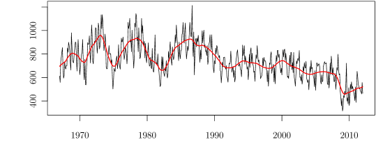
Fig. 4 shows that the form of trend is complex. This causes impossibility to obtain the full decomposition of the time series at once. Therefore, let us perform the decomposition sequentially. First, let us extract trend. Since for such changing form of the trend its extraction is similar to smoothing, we start with choosing minimally possible window length which in this case is $L=12$. The reason for this choice of window length is similar to that in moving averaging procedure: for smoothing the time series containing a periodic component, the window length should be divisible by the period.

Fragment 4.4 performs the decomposition and displays the information about the resulting ssa-object.

Fragment 4.4 “MotorVehicle”, 1st stage: decomposition

s1 <- ssa(MotorVehicle, L=12)
# Look inside ’s’ object to see, what is available.
summary(s1)

This is an example of the output of summary(s1):

Call:
ssa(x = MotorVehicle, L = 12)
Series length: 541,    Window length: 12,    SVD method: eigen
Computed:
Eigenvalues: 12,       Eigenvectors: 12,     Factor vectors: 0
Pre-cached: 0 elementary series (0 MiB)
Overall memory consumption (estimate): 0.005791 MiB

The SVD method “eigen” was chosen by default, since the window length is small and therefore fast SVD methods are not effective. Since the pre-caching is implemented in Rssa, it is important to know what the elements are already calculated. You can see that there are 12 eigenvectors and 0 elementary reconstruction components.

Now let us look at the decomposition results in Fragment 4.5 for the component identification.

Fragment 4.5 “MotorVehicle”, 1st stage: visual information for grouping

# Plot of eigenvalues
plot(s1)
# Plot of eigenvectors
# Here ’idx’ argument denotes the indices of vectors of interest
plot(s1, type = "vectors", idx=1:6)
# Plot of elementary reconstructed series
# Here ’groups’ argument specifies the grouping
plot(s1, type = "series", groups = as.list(1:6))

Note that the plot of eigenvalues does not need additional calculations due to pre-caching, while the plot of elementary reconstructed components needs additional time for calculations (though such calculations are performed only once for a given set of elementary components). The repeated call of summary(s1) shows that Precached: 6 elementary series (0.02497 MiB).

Figure 2: “MotorVehicle”, 1st stage: eigenvectors ($L=12$)

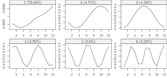
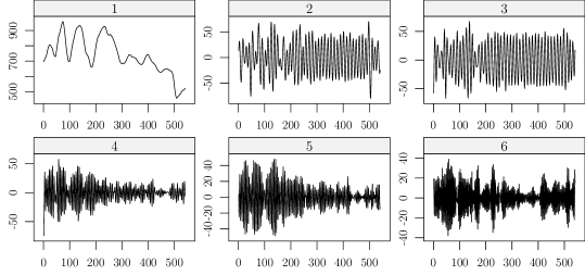
The graph of eigenvalues is not informative here and just reflects a large contribution of the leading eigentriple. Fig. 2 shows the form of the six leading eigenvectors. The leading eigenvector has almost constant coordinates and therefore it corresponds to a pure smoothing by the Bartlett filter (see Golyandina et al. (2012) and Golyandina and Zhigljavsky (2013)). The result of reconstruction by each of the six eigentriples is depicted in Fig. 3. Both figures confirm that the first eigentriple corresponds to the trend, the other eigentriples contain high-frequency components and therefore are not related to the trend. The trend from Fig. 4 is exactly the trend produced by one leading eigentriple and coincides with the first reconstructed component in Fig. 3. The trend can be reconstructed by the code from Fragment 4.6.

Fragment 4.6 “MotorVehicle”, 1st stage: reconstruction

res1 <- reconstruct(s, groups = list(1))
trend <- res1$F1

Figure 3: “MotorVehicle”, 1st stage: elementary reconstructed series ($L=12$)

Figure 4: “MotorVehicle”, 1st stage: initial series and estimated trend ($L=12$, ET1)

We have now extracted the trend and therefore the next stage is the extraction of seasonality from the residual obtained by the command res.trend <- residuals(res1). First, let us look at the periodogram (Fig. 5) by call spec.pgram(res.trend, detrend = FALSE, log = "no"). We see that the seasonality consists of sine waves with periods 12, 6, 4, 3, 2.4. Let us extract them by the SSA.

Figure 5: “MotorVehicle”, 2nd stage: periodogram of the series (i.e., of the residual at the 1st stage)

For better separability, we take the window length $L=264$ as the maximal window length $L$ such that $L\leq N/2$ and $L$ is divisible by 12.

Fragment 4.7 “MotorVehicle”, 2nd stage: decomposition and visual information

s2 <- ssa(res.trend, L=264)
plot(s2)
plot(s2, type = "paired", idx = 1:12, plot.contrib = FALSE)
# Calculate the w-correlation matrix using first 30 components.
# Here groups argument as usual denotes the grouping used.
w <- wcor(s, groups = as.list(1:30))
plot(w)

The code summary(s2) shows the chosen method SVD method: nutrlan and the number of calculated eigenvalues and eigenvectors, which is 50 (default).

Figure 6: “MotorVehicle”, 2nd stage: eigenvalues ($L=264$)

Figure 7: “MotorVehicle”, 2nd stage: scatterplots for eigenvector pairs ($L=264$)

Figure 8: “MotorVehicle”, 2nd stage: $\mathbf{w}$-correlation matrix ($L=264$)

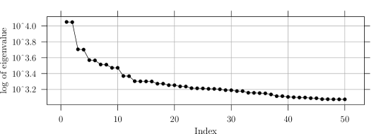
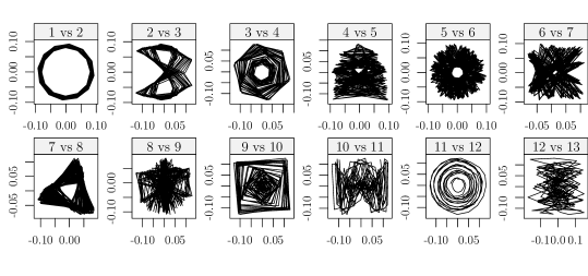
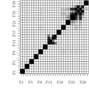
For proper identification of the sought sine waves, we will use the graph of eigenvalues, scatterplots of eigenvectors and $\mathbf{w}$-correlation matrix of the elementary components. In Fig. 6 we see several steps produced by approximately equal eigenvalues. Each step is likely to be yielded by a pair of eigenvectors which correspond to a sine wave. Fig. 7 confirms our guess. One can see six almost regular polygons. ET1–2, ET3–4, ET5–6, ET7–8 and ET9–10 correspond to periods 12, 6, 2.4, 3, 4, which are produced by the seasonality and are clearly explained by the periodogram (Fig. 5). The components are ordered in accordance with the ordering of the periodogram values at these frequencies. Fig 8 shows that the considered pairs of components are highly correlated within and are almost not correlated between. Note that there is one more pair of eigentriples ET11–12 which satisfies the same properties. Since this pair corresponds to the period 16, which is not interpretable for monthly data, we refer it to noise. The estimation of periods was performed by the function parestimate and the results are

> parestimate(s, 1:12, method = "esprit-ls")$periods
 [1]  2.996167  -2.996167  12.008794 -12.008794  2.398670  -2.398670
 [7] 16.198097 -16.198097   5.982904  -5.982904  4.014053  -4.014053
> parestimate(s, 11:12, method = "pairs")
 [1] 15.9677

Let us present the results of the series decomposition.

Fragment 4.8 “MotorVehicle”, 2nd stage: reconstruction and plotting of the results

res2 <- reconstruct(s2, groups=list(1:10))
seasonality <- res2$F1;
res <- residuals(res2);
# Extracted seasonality
plot(res2, add.residuals = FALSE, col = c("black", "red"))
# Result of Sequential SSA
plot(res2, base.series = res1)
# Seasonally adjusted series
plot(MotorVehicle-seasonality, type=’l’)

Figure 9: “MotorVehicle”, 2nd stage: the series and the extracted seasonal component

The extracted seasonality (ET1–10) is depicted in Fig 9. Slow change of sine wave phases seen in Fig. 7 yields a periodic behavior of complex form. Fig. 10 shows the resultant decomposition of both stages of Sequential SSA. Note that the obtained noise residuals are heterogeneous. As an auxiliary result, we obtain also seasonally adjusted series (Fig. 11).

Figure 10: “MotorVehicle”: Series and its trend-periodic-residuals decomposition

Figure 11: “MotorVehicle”: Seasonally adjusted series

Finally, let us demonstrate how to estimate the variance of the heterogeneous noise. The procedure is based on two observations: first, the variance is equal to the expectation of squared residuals; second, for stochastic process the trend is its expectation. Therefore, the variance can be estimated as the trend of squared residuals. This trend can be extracted by SSA with small window length and reconstructed by the leading eigentriple. The choice of window length makes affects the level of detail with which we see the extracted trend. The choice $L=30$ provides an appropriate trend. The result of Fragment 4.9 is depicted in Fig. 12 containing the residuals with standard deviation bounds.

Fragment 4.9 “MotorVehicle”: finding noise envelope

s.env <- ssa(res^2, L=30)
rsd <- sqrt(reconstruct(s.env, groups=list(1))$F1)
plot(res, type=’l’); lines(rsd, type=’l’); lines(-rsd, type=’l’)

Figure 12: “MotorVehicle”: Residuals with envelopes

Remark 2

For stationary time series the use of Toeplitz SSA is appropriate. In the described example, it makes no sense to apply Toeplitz SSA for trend extraction. Generally, it can be applied to extraction of seasonality via the call s <- ssa(res.trend, L=264, kind="toeplitz-ssa"). However, the result of decomposition is worse, since the seasonal behavior is changing in time. Note that the ordering of eigentriples by eigenvalues of the matrix $\mathbf{S}$ and their contribution to the decomposition differ. The values of s$lambda are equal to the contribution values, while the ordering is performed by eigenvalues. Therefore the graph plot(s) can be not-monotonic.

5 SSA forecasting with R

5.1 Typical code

After the decomposition has been performed forecasting becomes available. Rssa implements two methods of forecasting, recurrent and vector forecasts.

Fragment 5.1 “co2”: forecasting

# Decomposition stage
s <- ssa(co2, L = 120)
# Recurrent forecast, the result is the forecasted values only
# The result is the set of forecasts for each group
for1 <- rforecast(s, groups = list(1, c(1,4), 1:4, 1:6), len = 12)
matplot(data.frame(for1), type=’b’, pch = c(’1’,’2’,’3’,’4’))
# Recurrent forecast, the forecasted points added to the base series
for1a <- rforecast(s, groups = list(1, c(1,4), 1:4, 1:6), len = 36,
                  only.new = FALSE)
# Plot of the forecast based on the second group c(1,4)
plot(cbind(co2, for1a$F2), plot.type=’single’, col=c(’black’,’red’))
# Vector forecast
for2 <- vforecast(s, groups = list(1:6), len = 12, only.new = FALSE)
plot(cbind(co2, for2$F1), plot.type=’single’, col=c(’black’,’red’))
# Confidence intervals, they can be calculated for one group only
for3 <- bforecast(s, group = 1:6, len = 12, type = "recurrent")
plot(for3, plot.type="single", col=c("black","red","red"))

Alternatively, one can use the all-in-one function forecast which serves as a wrapper over rforecast, vforecast and bforecast and yields the output compatible with the forecast package (Hyndman, 2012). This way, one can use convenient graphic tools implemented in the forecast package to plot the forecast results. See Fragment 5.7 as an example of this.

Like the reconstruct function, all the forecasting routines try to use the attributes of the initial series for the resulting series (in particular, they try to add to the result the time index of the series). Unfortunately, this cannot be done in class-neutral way as it is done in the reconstruct case and needs to be handled separately for each possible type of time series. The forecasting routines know how to impute the time indices for some standard time series classes like ts and zooreg.

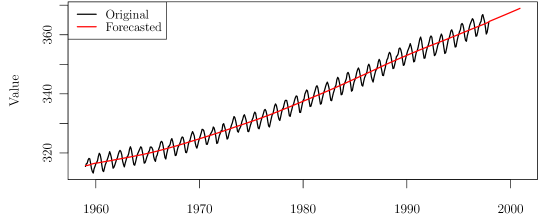
The forecast for trend (ET1 and ET4) is shown on Fig. 13 together with the initial series.

Figure 13: “co2”: trend forecast

In addition to forecasting, this block of Rssa functions provides tools for analyzing the forecasting LRR (Fragment 5.2). The roots are ordered by modulus since typically (but not always) the signal roots have maximal moduli (see Usevich (2010) for theoretical results about signal and extra roots).

Fragment 5.2 “co2”: linear recurrence relation

num <- 1:6
lrr.coef<-lrr(s, group = num)
r <- roots(lrr.coef)
# Plot of roots against the unit circle
plot(lrr.coef)

For description of the forecast behavior, the signal roots of the characteristic polynomial of the forecasting LRR and their parametric form should be found. For parameter estimation (frequency and damping rate) code of Fragment 5.3 can be used.

Fragment 5.3 “co2”: parameter estimation

print(2*pi/Arg(r[num]))
print(Mod(r[num]))
parestimate(s, 1:6, method = "esprit-ls")
parestimate(s, c(2:3,5:6), method = "esprit-ls")

The result of estimation through the LRR roots is

> print(2*pi/Arg(r[num]))
[1] 5.999366  -5.999366  11.996071 -11.996071      Inf      Inf
> print(Mod(r[num]))
[1] 1.000575   1.000575   1.000385   1.000385 1.000354 0.985554

All these roots are likely to be related to the signal. Results of application of the ESPRIT confirm this. This means that the explicit form of the forecast is the sum of half of year and annual sine waves with almost constant amplitude and also a trend approximated by the sum of two exponentials.

To find proper parameters of the method, testing of the forecasting formulas can be performed. The code from Fragment 5.4 shows how to implement the function to see the dependence of the forecasting accuracy on the window length and on the number of the selected components.

Fragment 5.4 Function for sliding forecasts

forecast.check <- function(F,
                           groups,
                           forecast.len = 1, sliding.len = N %/% 4,
                           ...,
                           type = c("recurrent", "vector")) {
  type <- match.arg(type)

  N <- length(F)
  K.sliding <- N - sliding.len - forecast.len + 1

  r <- matrix(nrow = K.sliding, ncol = length(groups))
  f.fun <- if (identical(type, "vector")) vforecast else rforecast
  for (i in 1:K.sliding) {
    F.train <- F[seq(from = i, len = sliding.len)]
    F.check <- F[seq(from = sliding.len + i, len = forecast.len)]
    s <- ssa(F.train, ...)
    for (idx in seq_along(groups)) {
      group <- groups[[idx]]
      f <- f.fun(s, groups = list(group), len = forecast.len)[[1]]
      r[i, idx] <- mean((f - F.check)^2)
    }
  }
  apply(r, 2, mean)
}

Fragment 5.5 contains examples showing how to use sliding forecasts for choosing the parameters. Commented lines show other reasonable choice for the corresponding variables. Length of sliding subseries equals 360, while the series length is equal to 468. Choice fl <- 1 corresponds to 108 one-step ahead forecasts (short-term forecasting), choice fl <- 108 corresponds to one 108-step ahead forecast (long-term forecasting).

Fragment 5.5 “co2”: dependence of forecast accuracy on choice of parameters

Lmin <- 24; N <- length(co2); ns <- 360
fl <- N-ns # fl <- 1
# groups <- list(1:6, 1:10, 1:15, 1:20)
groups <- list(c(1,4), 1:4, 1:6, c(1:6, 14, 15))
Lseq <- seq(Lmin, ns-Lmin, by = 6)
fcL <- function(L) forecast.check(co2, groups,
                                  forecast.len=1, sliding.len = ns,
                                  L = L, neig = 20, type="vector")
m <- sapply(Lseq, fcL)
matplot(time(co2)[Lseq], t(m),
        type = "l", col=c("red","green","blue","black"))

5.2 Case study

Let us consider the same example “MotorVehicle”. Since the trend has complex structure, it makes sense to forecast the trend and seasonality separately.

We start with forecasting the seasonality. Fragment 5.6 performs forecasts by recurrent and vector methods.

Fragment 5.6 “MotorVehicle” seasonality: forecasting

s1 <- ssa(MotorVehicle, L=12)
trend <- reconstruct(s1, groups = list(1))
res.trend <- residuals(trend); trend <- trend$F1
s2 <- ssa(res.trend, L=264)
frec <- rforecast(s2, groups = list(1:10), len = 60)$F1
fvec <- vforecast(s2, groups = list(1:10), len = 60)$F1
plot(cbind(frec, fvec), plot.type = "single", col=c("black","red"))

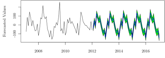
The results are stable enough and the difference between recurrent and vector forecasts is very small. To estimate the forecasting error, the bootstrap confidence intervals for the forecasted component can be calculated. This can be done with the help of the function bforecast or of its wrapper forecast for using the plotting facilities from forecast package, see Fragment 5.7.

Fragment 5.7 “MotorVehicle” seasonality: bootstrap confidence intervals

f <- forecast(s2, group = 1:10, len = 60,
              method = "bootstrap-recurrent")
plot(f, include = 60, shadecols = "green")

The confidence bounds are depicted in Fig. 14. Certainly, at least approximate independence and identical distribution of residuals should be checked before using confidence intervals based on these assumptions.

Figure 14: “MotorVehicle” seasonality: bootstrap confidence intervals

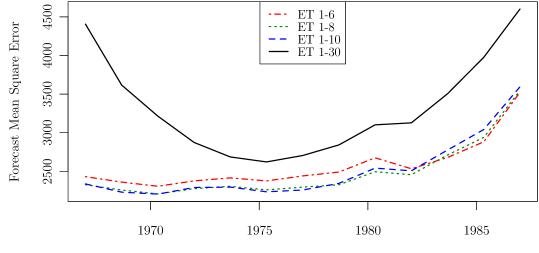
Let us check, if the removal of the starting period of the time series can improve accuracy.

Fragment 5.8 “MotorVehicle” seasonality: dependence of forecast accuracy on number of removed points

N <- length(MotorVehicle)
groups <- list(1:6, 1:8, 1:10, 1:30)
Nstart <- seq (1, 241, 20);
fcT <- function(NN)
  forecast.check(res.trend[NN:N], groups,
                 forecast.len = 12, sliding.len = 240,
                 L = 120, type="recurrent", svd.method="eigen")
m <- sapply(Nstart, fcT)
matplot(time(MotorVehicle)[Nstart], t(m),
        type = "l", col=c("red","green","blue","black"))

Fragment 5.8 uses the function defined in Fragment 5.4. One can see in Fig. 15 that it is better to use the whole time series and perform the forecasting based on ET1–8 or ET1–10.

Figure 15: “MotorVehicle” seasonality: dependence of forecast accuracy on number of removed points

Totally different situation takes place with the trend forecast. Since the trend possibly has a structure changing in time, it is unreasonable to use the whole trend for forecasting. Therefore, we need to find the last point of the structure change.

Probably, the last point of structure change is 2009 (crisis). Therefore, we make a forecast using the data from the last 3 years, that is, the last 36 points (Fragment 5.9).

Fragment 5.9 “MotorVehicle” trend: forecasting of last 3 years behavior

trend.end1 <- ts(trend[506:541],
                end = end(trend), frequency = frequency(trend))
s.end1 <- ssa(trend.end1)
frec1 <- rforecast(s.end1, groups = list(1),
                  len = 24, only.new = FALSE)$F1
plot(cbind(trend.end1, frec1), plot.type="single",
     col=c("black","red"))

If we consider a longer time period for forecasting (Fragment 5.10), then we will see a totally different forecast (Fig. 16).

Fragment 5.10 “MotorVehicle” trend: forecasting of last 22 years behavior

trend.end2 <- ts(trend[270:541],
                end = end(trend), frequency = frequency(trend))
s.end2 <- ssa(trend.end2)
frec2 <- rforecast(s.end2, groups = list(1:4),
                  len = 24, only.new = FALSE)$F1
plot(cbind(trend.end2, frec2), plot.type="single",
     col=c("black","red"))

Figure 16: “MotorVehicle” trend: forecasting of last 3 and 22 years behavior

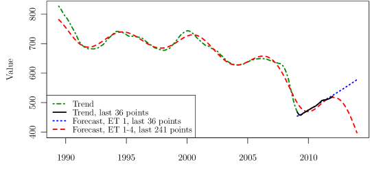
To choose the proper forecast, additional macroeconomic analysis is necessary.

References

- Anderson et al. (1999) Anderson, E., Bai, Z., Bischof, C., Blackford, S., Demmel, J., Dongarra, J., Du Croz, J., Greenbaum, A., Hammarling, S., McKenney, A., Sorensen, D., 1999. LAPACK Users’ Guide, 3rd Edition. SIAM, Philadelphia, PA.
- Badeau et al. (2005) Badeau, R., Richard, G., David, B., 2005. Fast adaptive ESPRIT algorithm. In: Statistical Signal Processing’05. Bordeaux, France, pp. 289–294.
- Elsner and Tsonis (1996) Elsner, J. B., Tsonis, A. A., 1996. Singular Spectrum Analysis: A New Tool in Time Series Analysis. Plenum.
- Ghil et al. (2002) Ghil, M., Allen, R. M., Dettinger, M. D., Ide, K., Kondrashov, D., Mann, M. E., Robertson, A., Saunders, A., Tian, Y., Varadi, F., Yiou, P., 2002. Advanced spectral methods for climatic time series. Rev. Geophys. 40 (1), 1–41.
- Golub and Van Loan (1996) Golub, G. H., Van Loan, C. F., 1996. Matrix computations (3rd ed.). Johns Hopkins University Press, Baltimore, MD, USA.
- Golyandina (2010) Golyandina, N., 2010. On the choice of parameters in singular spectrum analysis and related subspace-based methods. Stat. Interface 3 (3), 259–279.
- Golyandina et al. (2001) Golyandina, N., Nekrutkin, V., Zhigljavsky, A., 2001. Analysis of Time Series Structure: SSA and Related Techniques. Chapman&Hall/CRC.
- Golyandina et al. (2012) Golyandina, N., Pepelyshev, A., Steland, A., 2012. New approaches to nonparametric density estimation and selection of smoothing parameters. Comput. Stat. Data Anal. 56 (7), 2206–2218.
- Golyandina and Zhigljavsky (2013) Golyandina, N., Zhigljavsky, A., 2013. Singular Spectrum Analysis for time series. Springer Briefs in Statistics. Springer.
- Hassani et al. (2009) Hassani, H., Heravi, S., Zhigljavsky, A., 2009. Forecasting European industrial production with singular spectrum analysis. Int. J. Forecast. 25 (1), 103 – 118.
- Hyndman (2012) Hyndman, R. J., 2012. forecast: Forecasting functions for time series and linear models. R package version 3.25, with contributions from Slava Razbash and Drew Schmidt.
- Jenkins and Traub (1970) Jenkins, M., Traub, J., 1970. A three-stage variable-shift iteration for polynomial zeros and its relation to generalized rayleigh iteration. Numerische Mathematik 14, 252–263.
- Keeling and Whorf (1997) Keeling, C. D., Whorf, T. P., 1997. Atmospheric CO2 concentrations — Mauna Loa Observatory, Hawaii, 1959-1997. Scripps Institution of Oceanography (SIO), University of California, La Jolla, California USA 92093-0220.
- Korobeynikov (2010) Korobeynikov, A., 2010. Computation- and space-efficient implementation of SSA. Stat. Interface 3 (3), 357–368.
- Larsen (1998) Larsen, R. M., 1998. Efficient algorithms for helioseismic inversion. Ph.D. thesis, University of Aarhus, Denmark.
- Roy and Kailath (1989) Roy, R., Kailath, T., 1989. ESPRIT: estimation of signal parameters via rotational invariance techniques. IEEE Trans. Acoust. 37, 984–995.
- U.S. Bureau of Economic Analysis (2012) U.S. Bureau of Economic Analysis, 2012. Table 7.2.5s. Auto and Truck Unit Sales Production Inventories Expenditures and Price.
- Usevich (2010) Usevich, K., 2010. On signal and extraneous roots in Singular Spectrum Analysis. Stat. Interface 3 (3), 281–295.
- Yamazaki et al. (2008) Yamazaki, I., Bai, Z., Simon, H., Wang, L.-W., Wu, K., 2008. Adaptive projection subspace dimension for the thick-restart Lanczos method. Tech. rep., Lawrence Berkeley National Laboratory, University of California, One Cyclotron road, Berkeley, California 94720.
- Zeileis and Grothendieck (2005) Zeileis, A., Grothendieck, G., 2005. zoo: S3 infrastructure for regular and irregular time series. Journal of Statistical Software 14 (6), 1–27.