The Origin of Kepler’s Supernova Remnant

Abstract

It is now well established that Kepler’s supernova remnant is the result of a Type Ia explosion. With an age of 407 years, and an angular diameter of $\sim$ 4$\arcmin$, Kepler is estimated to be between 3.0 and 7.0 kpc distant. Unlike other Galactic Type Ia supernova remnants such as Tycho and SN 1006, and SNR 0509-67.5 in the Large Magellanic Cloud, Kepler shows evidence for a strong circumstellar interaction. A bowshock structure in the north is thought to originate from the motion of a mass–losing system through the interstellar medium prior to the supernova. We present results of hydrodynamical and spectral modeling aimed at constraining the circumstellar environment of the system and the amount of ⁵⁶Ni produced in the explosion. Using models that contain either 0.3M_☉ (subenergetic) or 1.0M_☉ (energetic) of ⁵⁶Ni, we simulate the interaction between supernova Ia ejecta and various circumstellar density models. Based on dynamical considerations alone, we find that the subenergetic models favor a distance to the SNR of $<$ 6.4 kpc, while the model that produces 1M_☉ of ⁵⁶Ni requires a distance to the SNR of $>$ 7 kpc. The X-ray spectrum is consistent with an explosion that produced $\sim$ 1M_☉ of ⁵⁶Ni, ruling out the subenergetic models, and suggesting that Kepler’s SNR was a SN 1991T-like event. Additionally, the X-ray spectrum rules out a pure $r^{-2}$ wind profile expected from isotropic mass loss up to the time of the supernova. Introducing a small cavity around the progenitor system results in modeled X-ray spectra that are consistent with the observed spectrum. If a wind shaped circumstellar environment is necessary to explain the dynamics and X-ray emission from the shocked ejecta in Kepler’s SNR, then we require that the distance to the remnant be greater than 7 kpc.

1. Introduction

Type Ia supernovae (SNe) are believed to be the thermonuclear explosion of a C+O white dwarf (WD) that is destabilized when its mass approaches the Chandrasekhar limit by accretion of material from a binary companion. After the central regions ignite, a burning front propagates outwards, consuming the entire star and leading to a characteristic ejecta structure with $\sim$ 0.7 M_☉ of Fe-peak nuclei (primarily in the form of ⁵⁶Ni that powers the SN light curve) in the inside, and an equal amount of intermediate mass elements on the outside. While the amount of ⁵⁶Ni can vary between $\sim$ 0.3 M_☉ and $\sim$ 1 M_☉, the stratification of the ejecta remains constant across SNe Ia subtypes (Mazzali et al., 2007). The simple structure of the ejecta results in uniform light curves and spectra and make SN Ia useful distance indicators (e.g., Riess et al., 1998; Perlmutter et al., 1999). Depending upon the nature of the WD companion, SN Ia progenitors are divided into either single degenerate (Hachisu et al., 1996) or double degenerate cases (Iben & Tutukov, 1984; Webbink, 1984). Finding clear evidence supporting one of these two scenarios has become a cornerstone in stellar astrophysics, as unknown evolutionary effects associated with the progenitors may introduce systematic trends that could limit the precision of cosmological measurements based on SN Ia (Howell et al., 2009).

Most Type Ia supernova remnants (SNRs) reflect the simplicity of the explosion. Galactic SNRs such as Tycho and SN 1006 appear remarkably symmetric (Warren et al., 2005; Cassam-Chenaï et al., 2008), unlike their core–collapse counterparts, such as Cas A (DeLaney et al., 2010; Lopez et al., 2011; Hwang & Laming, 2012) or younger extragalactic SNe such as SN 1980K or SN 1993J (Milisavljevic et al., 2012). The morphology and X-ray spectra of SNRs with known ages and a Type Ia classification also indicate that the progenitors do not modify their surroundings in a strong way – in particular, while absorption features seen in the spectra of Type Ia SNe suggest small cavities of radius $\gtrsim$ 10¹⁷ cm (Patat et al., 2007; Blondin et al., 2009; Borkowski et al., 2009; Simon et al., 2009; Sternberg et al., 2011), there is little evidence for large ($r$ $\sim$ 3 – 30 pc) wind-blown cavities around the explosion site (Badenes et al., 2007). However, Williams et al. (2011) recently showed that the candidate Type Ia RCW 86 is currently interacting with a cavity wall and that the cavity has a radius of $\sim$ 12 pc, in the middle of the range of sizes expected from the accretion wind models (Badenes et al., 2007). The lack of a sizeable population of Ia SNR inside of cavities is particularly relevant as the current paradigm for SN Ia progenitors in the single degenerate channel predicts fast, optically thick outflows from the WD surface which would leave behind such cavities (e.g. Hachisu et al., 1996). Additionally, the dynamical and spectral properties of young Ia SNRs like Tycho and 0509–67.5 are more consistent with an interaction with a constant density interstellar medium (ISM) (Badenes et al., 2006, 2008).

A notable exception to this is Kepler’s SNR (G4.5+6.8; Kepler), shown in X-rays in Figure 1. Kepler’s SNR has recently been firmly established as the remnant of a Type Ia SN, based on the O/Fe ratio observed in the X-ray spectrum (Reynolds et al., 2007). However, unlike many other Type Ia SNRs, the morphology of this $\approx$ 400 yr old remnant shows a strong bilateral symmetry, and optical observations reveal clear signs of an interaction between the blastwave and a dense, nitrogen–enhanced circumstellar shell with a mass of $\sim$ 1M_☉ (Vink, 2008). Near infrared observations also show evidence for circumstellar knots akin to the quasi-stationary floculi of Cassiopeia A (Gerardy & Fesen, 2001). This suggests that either the progenitor of Kepler’s SN or its binary companion might have been relatively massive, creating a bowshock shaped circumstellar medium (CSM) structure as the system lost mass and moved against the surrounding ISM. Borkowski et al. (1992) found values of $\dot{M}$ $\sim$ 5$\times$ 10^-6 M_☉ yr^-1 and v_wind = 15 km s^-1 are required in order to explain the morphology of Kepler’s bowshock. While it is likely that not all progenitor scenarios for SNe Ia are the same, the dense CSM wind required to create the observed morphology appears to be in conflict with observations of the recent nearby SN Ia 2011fe in M101 (Nugent et al., 2011; Li et al., 2011). In the case of 2011fe, the radio and X-ray observations place constraints on the circumstellar environment with $n_{\mathrm{CSM}}$ $\lesssim$ 6 cm^-3, or in the case of a stellar wind, $\dot{M}$ $\lesssim$ 6$\times$10^-10 M_☉ yr^-1 (Horesh et al., 2012; Chomiuk et al., 2012). It is worth noting, however, that the recent observations of SN 2011fe probe spatial scales of $\sim$ 10¹⁶ cm, corresponding to the last $\sim$ 100–1000 yr of the progenitor’s evolution, while the blastwave of Kepler’s SNR is probing the mass-loss history 10⁵ – 10⁶ yr ago.

Located well above the Galactic plane, the SNR has an angular size of 2$\arcmin$ in radius, but the distance is poorly constrained. Reynoso & Goss (1999) used H I absorption to estimate a distance of 4.8 $<$ D_SNR $<$ 6.4 kpc, while Sankrit et al. (2005) estimate that the SNR is somewhat closer, with a lower limit of 3.0 kpc on the distance, based on the width of the H$\alpha$ line and proper motion measurements. The non-detection of TeV $\gamma$-rays by HESS (F_γ $<$ 8.6 $\times$ 10^-13 erg cm^-2 s^-1) places a lower limit on the distance to Kepler of $\sim$ 6 kpc (Aharonian et al., 2008) assuming a model for the gamma-ray emission (Berezhko et al., 2006), for a normal Ia SN. To match the angular size, the distance would have to be even greater than 6 kpc ($\gtrsim$ 7 kpc) if the SN were more energetic than a normal Ia, or else the blastwave would have to expand into a CSM with considerable density. Vink (2008) measured the velocity of the SNR forward shock and estimated $v_{s}$ = 4200$d_{4\mathrm{kpc}}$ km s^-1 and concluded that the distance must be $\gtrsim$ 6 kpc or otherwise the SN was subenergetic. The distance estimates are incompatible with one another: either 3.0 $<$ D_SNR $<$ 6.4 kpc, or D_SNR $>$ 7 kpc, based on the non-detection of TeV gamma-rays, an important new constraint. Given the uncertainty on the distance, the blastwave has a radius between 1.75 $\geq$ R_FS $\geq$ 3.7 pc, or R_FS $>$ 4.1 pc.

Here we present hydrodynamical simulations of Type Ia SN ejecta interacting with an external medium shaped by a circumstellar wind. Combining models for the pre-supernova mass-loss with models for the ejecta density distribution and composition, we simultaneously fit both the morphology of the SNR and the observed X-ray spectrum within the observable constraints– the age and angular size of the SNR along with the bulk spectral properties. Since the circumstellar environment is complicated by the bowshock structure in the north, we focus our attention on the southern portion of the SNR (see Fig. 1), in an attempt to minimize the number of free parameters in our hydrodynamical simulations. Based on our joint hydrodynamical and spectral fits, we conclude that Kepler was a luminous Type Ia SN. If the SNR is expanding into a stellar wind we require a distance to Kepler of $>$ 7 kpc. If, on the other hand, the SNR is expanding into a uniform medium, the distance is somewhat closer, $\sim$ 5 kpc.

2. X-ray Emission from Kepler’s SNR

A 750ks Chandra image of Kepler’s SNR (PI: S. Reynolds) is shown in Figure 1, with the X-ray emission from the pie-sliced region shown in Figure 2 (left). As shown in Fig 2 (left), the X-ray spectrum is dominated by emission from Fe K and Fe L, as well as emission from intermediate mass elements such as silicon, sulfur, and argon. The amount of iron emission in the spectrum is a key constraint on the explosion, as it will allow us to discriminate between Type Ia explosion models (Badenes et al., 2005). Besides emission from the shocked ejecta, there is also emission from circumstellar material– mainly oxygen and neon, which overlaps with the L-shell iron emission (Reynolds et al., 2007), as well as nonthermal continuum which contributes to the emission above a few keV (Reynolds et al., 2007; Cassam-Chenaï et al., 2008). In the subsequent discussion on the fits to the spectrum, we do not account for either the contribution from the swept up circumstellar material or nonthermal emission in the spectral models– the contribution by shocked circumstellar material to the thermal X-ray emission is small and accounts for only a few percent of the total emission (Reynolds et al., 2007), while the nonthermal emission serves to raise the continuum above $\sim$ 4 keV. The processes that lead to the nonthermal emission could alter the thermal spectrum (Patnaude et al., 2009, 2010), but those affects have been shown to be small, particularly in young SNRs (Patnaude et al., 2010). Interesting characteristics of the spectrum include: the presence or absence of emission from iron, which will constrain the explosion energetics; the centroids of K–shell emission lines, which constrains the ionization state of the shocked gas; and flux ratios of individual lines, such as K$\alpha$ to H-like Ly$\alpha$, which constrain the density of the circumstellar material.

The spectra from the combined 750ks observation shown in Figure 1 was extracted from the Level 2 Chandra event list using CIAO 4.1, and weighted response matrices were computed using CalDB version 4.1.3. The broadband spectrum (Fig. 2, left) shows significant emission from both Fe L and Fe K (Reynolds et al., 2007). Given the complexity of the Fe L emission at $\sim$ 1 keV, we focus only on those emission lines above 1.5 keV, as they are well separated from neighboring lines. To measure the emission line centroids, we modeled the spectrum as a powerlaw continuum with a series of Gaussians for each emission line. The spectral fit is shown in Figure 2 (right). We chose to model the continuum as a powerlaw since Cassam-Chenaï et al. (2008) showed that much of the continuum emission in Kepler is nonthermal in nature (see Figs. 6 and 8 of Cassam-Chenaï et al., 2008). For the spectral fits, we used XSPEC Version 11.3.2ag. We used a region nearby the supernova remnant for a local background subtraction. Since we are only fitting the data above $\sim$ 1.5 keV, we do not include absorption in our spectral fits. Reynolds et al. (2007) found an absorbing column of N_H = 5.2 $\times$ 10²¹ cm^-2 by fitting featureless regions along the remnant’s rim to an absorbed srcut model. Fitting only the data above 1.5 keV, we were unable to constrain the column density. However in the subsequent sections where we compare our hydrodynamical and spectral models to the data, we assume a column of 5.2 $\times$ 10²¹ cm^-2 so that we may compare the computed X-ray emission below 1.5 keV directly to the data.

The results of our centroid fits are listed in Table 1. The key results in Table 1 are the line centroids, and in the subsequent discussion, we will focus on the line centroids of of Si K$\alpha$, S K$\alpha$, and Fe K$\alpha$. We also point out in Figure 2 (right) that there is little emission at 2 keV from Si XIV Ly$\alpha$. This is confirmed in our spectral analysis where we are only able to set an upper limit on the Si XIV Ly$\alpha$ emission from shocked ejecta in the south. The lack of emission at this energy will be used to constrain the CSM structure and density.

3. Hydrodynamical Modeling

In this section, we present results from a modeling effort where we have coupled the hydrodynamics to a nonequilibrium ionization (NEI) calculation to produce joint spectral and dynamical fits to Kepler’s SNR. We describe, in general terms in § 3.1 the formation of the bowshock structure in the north of Kepler and how it can be used to constrain the mass-loss parameters of the progenitor system. We also describe how the choice of Ia explosion model (e.g. the explosion energy and amount of ⁵⁶Ni that is synthesized) imposes a constraint on the uncertain distance to the SNR. In the subsequent sections, we compare the bulk spectral properties of Kepler’s SNR to those predicted by our spectral models.

3.1. Morphology of Kepler’s SNR in the Context of a CSM Interaction

The presence of a bowshock and shell of circumstellar material in the north of Kepler’s SNR suggests that there was an outflow from the progenitor or its companion prior to the explosion. This is because the bowshock can only form at a converging flow, in this case a wind interacting with the interstellar medium, where the ISM has a net inflow velocity relative to the progenitor, due to the progenitor’s systemic velocity through the ISM. Chiotellis et al. (2012) recently modeled the dynamics of the SNR blastwave through the bowshock and concluded that the dynamics of the SNR blastwave are consistent with the presence of a bowshock. We can use estimates for the location of the bowshock stagnation point as a constraint on the wind parameters. Generally, the location of the stagnation point, $r_{0}$, is written as (e.g. Huang & Weigert, 1982; Borkowski et al., 1992):

$$r_{0}=1.78\times 10^{3}\left(\frac{\dot{M}v_{\mathrm{wind}}}{n_{\mathrm{amb}}u_{\star}^{2}}\right)^{1/2}\mathrm{pc}\ ,$$ (1)

where $\dot{M}$ is the mass-loss rate, $v_{\mathrm{wind}}$ is the wind speed, $n_{\mathrm{amb}}$ is the ambient ISM density, and $u_{\star}$ is the systemic velocity of the star. In order to explain the large distance above the Galactic plane, the progenitor likely had a large systemic velocity, $u_{\star}$ $\sim$ 250 km s^-1 (Bandiera, 1987), a notion confirmed by the high proper motion and radial velocities of nitrogen-rich knots in the remnant, as well as the narrow component of the H$\alpha$ line in the nonradiative shock. Borkowski et al. (1992) estimated that the undisturbed ISM material had a density of 10^-3 – 10^-4 cm^-3, corresponding to the hot component of the ISM (McKee & Ostriker, 1977). Equation 1 can be inverted to estimate the mass-loss rate of the wind:

$$\dot{M}=3.15\times 10^{-7}\frac{n_{\mathrm{amb}}u_{\star}^{2}}{v_{\mathrm{wind}}}\left(\frac{r_{0}}{\mathrm{pc}}\right)^{2}\ .$$ (2)

Given the uncertainty of greater than a factor of two on the distance, the stagnation point is located at a radius of 2–4 pc, similar to the 2–3 pc assumed by Borkowski et al. (1992). The amount of mass in the shell is $\approx$ 1 M_☉. Chiotellis et al. (2012) have suggested that the nitrogen–rich knots in the CSM, combined with the solar mass of material in the shell, argue in favor of the CSM being sculpted by the outflow from an asymptotic giant branch (AGB) star. The mass-loss rates from AGB stars can vary over several orders of magnitude, but the velocity of the wind is generally 10–20 km s^-1 (Schöier & Olofsson, 2001; Olofsson et al., 2002; Ramstedt et al., 2009). Using this range in velocity combined with the range in the radius of the stagnation point yields mass-loss rates of 10^-6 – 10^-5 M_⊙ yr^-1.

To model a CSM wind, the mass-loss rate and wind velocity are all that are required, since $\rho_{\mathrm{amb}}$ = $Ar^{-2}$ where the wind normalization $A$ $=$ $\dot{M}$/(4$\pi$ $v_{\mathrm{wind}}$). We couple this model for the circumstellar environment to models for Type Ia SN ejecta from Badenes et al. (2003). We choose to focus on models DDTa (E_SN = 1.4$\times$10⁵¹ erg) and DDTg (E_SN = 0.9$\times$10⁵¹ erg). The choice of models is designed to encompass the diversity of Ia explosions (Badenes et al., 2008). In a constant density environment, the choice of explosion model does not significantly influence the radius and velocity of the forward shock as long as the kinetic energy is $\sim$ 10⁵¹ erg. In a wind environment, the difference in forward shock radius between an energetic and subenergetic model, where the ejecta is approximated as a powerlaw in velocity, is a little larger, since R_FS $\propto$ E${}_{\mathrm{SN}}^{2/(n-2)}$ rather than E${}_{\mathrm{SN}}^{2/n}$ (Chevalier, 1982). Of more interest is the resultant X-ray emission, which is influenced by the density and chemical composition of the ejecta. For instance, in the DDTa model, $\sim$ 1M_☉ of ⁵⁶Ni is produced, compared to 0.3M_☉ in the DDTg model. Since the ⁵⁶Ni decay is responsible for the iron observed in the ejecta, the amount of ⁵⁶Ni produced in the SN will profoundly affect the emitted X-ray spectrum.

Using the VH-1 hydrodynamics code, a numerical hydrodynamics code developed at the University of Virginia by J. Hawley, J. Blondin, and collaborators (e.g., Blondin & Lufkin, 1993), we modeled the expansion of the SN ejecta into the CSM wind to an age of 400 yr. We varied the wind speed between 10–20 km s^-1 and the mass-loss rate as described above. The parameter space results in a grid of models that relate the radius of the forward shock with the wind mechanical luminosity, $L_{\mathrm{wind}}$ = $\frac{1}{2}\dot{M}v_{\mathrm{wind}}^{2}$, for each explosion model. In Figure 3, we plot the shock radius as a function of wind luminosity for each combination of wind speed and mass-loss rate. Roughly speaking $R_{\mathrm{FS}}$ $\propto$ $L_{\mathrm{wind}}^{1/5}$ $\propto$ v${}_{\mathrm{wind}}^{2/5}$, for a given mass-loss rate. This is because the CSM density normalization is set by the wind speed – higher wind velocities transport the mass further away from the progenitor, while lower velocity winds result in more mass deposited closer to the progenitor. In the higher wind velocity models, the blastwave propagates further after 400 years since it has to move through less material.

As discussed earlier, the distance to Kepler is not well known, ranging from 3 – 6.4 kpc, or $>$ 7 kpc. In Figure 3, we also note the distance to Kepler on the right hand axis, using the measured angular radius of 2$\arcmin$. The upper limit of 6.4 kpc (Sankrit et al., 2005) on the distance rules out all DDTa models on dynamical considerations alone. However, if the distance is $>$ 7 kpc, as expected from the TeV gamma-ray non-detection, then most DDTa models are allowed, while a sizeable fraction of DDTg models ($\dot{M}$ $\gtrsim$ 6$\times$ 10^-6 M_☉ yr^-1) are no longer favored.

3.2. Spectral Fitting: Wind Models

To compare our grid of dynamical models to the observations of Kepler, we have generated synthetic X-ray spectra for the emission from shocked ejecta in our hydrodynamic simulations following the methods presented in (Badenes et al., 2003, 2005), using updated atomic data (Badenes et al., 2006), and including radiative and ionization losses as described in Badenes et al. (2007). In a constant density ambient medium, the synthetic spectra are controlled by three variables: the density of the ambient material, the SNR age, and the amount of collisionless heating between electrons and ions ($\beta$) at the reverse shock. For our models where $\rho_{\mathrm{amb}}$ $\propto$ $r^{-2}$, the X-ray emission is instead influenced by the wind normalization (which sets the density). Higher values of $\dot{M}$/(4$\pi$ $v_{\mathrm{wind}}$) will result in more circumstellar material closer to the explosion. We expect that this will lead to more collisional ionization in the shocked ejecta which will be directly reflected in the X-ray spectrum.

The ability of our synthetic spectra to reproduce the observations is limited by the quality of the atomic data used in the code. The data for K$\alpha$ blends are reasonably complete however, and we thus focus on those lines. As shown in Table 1, we have measured the line centroids and fluxes of several K$\alpha$ lines. These can be compared directly against the synthetic spectra from our models. We focus only on the brightest lines of silicon, sulfur, and iron, and note the following additional constraints on our models– (1): the presence of Fe K emission at $\sim$ 6.4 keV; (2): the absence of significant Si XIV Ly$\alpha$ emission at $\sim$ 2.0 keV; (3): the amount of Fe L emission below 1 keV, relative to oxygen suggests that the emission there is in fact ejecta and not shocked circumstellar material (Reynolds et al., 2007).

In Figure 4 (left, upper panel) we plot the X-ray spectrum from Figure 2 (left) compared against a subset of our spectral models. We plot the spectra from both the DDTa and DDTg models for a range of mass-loss rates, assuming wind velocities of 20 km s^-1. Given constraints (1) and (3) above, we can rule out the DDTg models since they do not produce enough iron to match the emission seen both at 6.4 keV and Fe L emission at $\sim$ 1 keV. By ruling out the DDTg models, we are also essentially ruling out the distance estimate of 3 $<$ D_SNR $<$ 6.4 kpc, if the blastwave is expanding into a $\rho_{amb}$ $\propto$ $r^{-2}$ wind. In contrast, some DDTa models do reproduce the Fe K$\alpha$ and Fe L emission. Those DDTa models with with $\dot{M}$ $<$ 4$\times$10^-6 M_☉ yr^-1 are ruled out since they produce very little emission at 6.4 keV, in conflict with the data.

In Figure 5 (left, upper panels), we plot the line centroids from the DDTa and DDTg models for various mass-loss rates for wind speeds of 20 km s^-1. The hatched region in each panel corresponds to the 90% confidence on the line centroid from the spectral fitting in Table 1. While we have previously ruled out the DDTg models in this wind scenario based on the absence of Fe emission, we are also forced to rule out those DDTa models that do produce Fe K emission as the predicted line centroids for nearly all models considered are at higher energies than what is measured.

Finally, and for comparison with other possible CSM models, we note that those DDTa models shown in Figure 4 that produce Fe K emission also result in significant Si XIV Ly$\alpha$ emission at $\sim$ 2.0 keV. This emission is not observed in the spectrum (Fig. 2), and our spectral fits only resulted in an upper limit on the Si XIV Ly$\alpha$ flux (Table 1). This is shown quantitatively in Figure 5 (right) where we plot the ratio of the modeled flux from Si K$\alpha$ to that from Si XIV Ly$\alpha$, for comparison against the measured ratio. In summary, based on the results of our comparisons between the observed and modeled bulk properties of the X-ray spectrum from the shocked ejecta, we must conclude that the X-ray emission from Kepler’s SNR is not consistent with what is expected from supernova ejecta interacting with a $\rho_{\mathrm{amb}}$ $\propto$ $r^{-2}$ wind as proposed by Chiotellis et al. (2012).

3.3. Spectral Fitting: Wind + Cavity Model

As discussed above, pure wind models do not provide a good fit to the X-ray spectrum. The reason is that the low wind velocities and moderate mass-loss rates that are required to match the SNR dynamics result in a significant amount of circumstellar material close to the explosion. Physically, this results in a stronger reverse shock being driven into the expanding ejecta, resulting in higher average charge states– this affects both the K$\alpha$ line centroid as well as the amount of Ly$\alpha$ emission. These are two measurable quantities which do not agree with the simple models described above.

The possibility exists that the circumstellar environment is more complicated than that of a simple $r^{-2}$ wind. Recurrent novae (e.g., Sokoloski et al., 2006; Wood-Vasey & Sokoloski, 2006) or optically thick accretion winds (e.g., Hachisu et al., 1996) from the white dwarf could carve out a cavity around the progenitor, even while the companion is losing mass to a slow and dense wind. We consider the formation of a small ($\sim$ 10¹⁷ cm) cavity inside the dense wind. The cavity could form in a number of ways (see Chomiuk et al., 2012, for a recent review), and time-variable Na I D absorption spectra indicate that cavities can have sizes $\gtrsim$ 10¹⁷ cm (Patat et al., 2007; Blondin et al., 2009; Simon et al., 2009; Sternberg et al., 2011). A small cavity such as this will not significantly alter the dynamics of the forward shock, but it will slow the ionization of the ejecta, resulting in lower charge states and dynamically younger shocked ejecta.

In the bottom panel of Figure 4 (left), we plot the synthesized X-ray emission from models where the wind has a small cavity carved out of it. Additionally, we show in the bottom panel of Figure 5 (left) the computed line centroids for these models. In the right hand panel of Figure 5, we show the modeled flux ratio of Si K$\alpha$ to Si XIV Ly$\alpha$ compared against the upper limit on the flux ratio from the X-ray spectrum, as a function of mass-loss rate. As shown in these plots, the line centroids (Si K$\alpha$ and S K$\alpha$) now agree with the measured values (for velocities $\lesssim$ 20 km s^-1). Additionally, these modified models show little Si XIV Ly$\alpha$ emission at $\sim$ 2 keV, as evidenced by the low flux ratios seen in the right hand panel, particularly for mass-loss rates less than 6$\times$10^-6 M_☉ yr^-1. We can thus conclude that these models are consistent with the observed X-ray spectrum.

When working within the dynamical constraints imposed by the DDTa models, we require a distance greater than 7 kpc, and a wind luminosity greater than $\sim$ 6$\times$10³² erg s^-1. Additionally, we require iron emission, agreement between the modeled and measured K$\alpha$ line centroids, and little or no Si XIV Ly$\alpha$ emission. The high mechanical wind luminosity rules out models with low values of $\dot{M}$, while the lower limit on the distance rules out the high mass-loss rate models. The presence of Si XIV Ly$\alpha$ emission in the modeled spectra rule out those models with $\dot{M}$ $\gtrsim$ 6$\times$10^-6 M_☉ yr^-1. We are left to conclude that a wind with a mass-loss rate of $\sim$ 4–6 $\times$10^-6 M_☉ yr^-1 and wind velocities $\sim$ 20 km s^-1 sculpted the CSM, and that a small cavity likely surrounded the progenitor, possibly caused by either recurrent novae or optically thick accretion winds that preceded the supernova.

3.4. Spectral Fitting: Constant Density Models

Finally, we consider models with a uniform ambient medium, with density $\rho_{\mathrm{amb}}$ = 1–5 $\times$ 10^-24 g cm^-3. Vink (2008) measured the expansion of Kepler’s SNR in the south and compared it against models for the expansion of a SNR blastwave in a constant density external medium. They found that models where $\rho_{\mathrm{ej}}$ $\propto$ $v^{-7}$ were able to reproduce the kinematics. However, they concluded that the kinematics of the blastwave in the south point to an explosion with E_SN $<$ 5 $\times$ 10⁵⁰ erg for the canonical distance of 4 kpc, assuming an ambient medium density of n_H = 1 cm^-3. Higher explosion energies work if the SNR is at a distance considerably greater than 4 kpc, or if the ambient medium density $>$ 10 cm^-3.

In Figure 4 (right), we show the computed X-ray emission for DDTa models in a constant density medium. As shown in Fig. 4, these models qualitatively reproduce the bulk features seen in the spectrum, and an ambient medium density of 2–5 $\times$ 10^-24 g cm^-3 seems to be able to reproduce both the line centroids as well as the line flux ratios. This is confirmed in Figure 6, where we see that models with densities of $<$ 3$\times$10^-24 g cm^-3 produce the required Si XIV Ly$\alpha$ emission and also predict line centroids in agreement with the measured values. For these models, the forward shock radii at 400 yrs range from 2.9 – 3.8 pc. For the measured angular radius of 2$\arcmin$, this corresponds to a distance to Kepler of 5 – 6.5 kpc, consistent with the distance estimate of Sankrit et al. (2005).

While the constant density models can explain the observed X-ray emission and also provide estimates for the distance to Kepler that are in agreement with proper motion measurements of Balmer filaments (Sankrit et al., 2005), it is difficult to reconcile a constant density CSM with the bowshock structure in the north. To form a bowshock, a converging flow is required between an outflow from the progenitor and the bulk motion of the ambient ISM (in the rest frame of the progenitor). Two alternative scenarios are considered: First, for either a wind that is not spherically symmetric but consists of equatorial and polar components (Owocki et al., 1994), or other non-spherical outflows, such as in the recurrent nova RS Oph (Sokoloski et al., 2006; Drake et al., 2009; Orlando et al., 2009), the CSM could be sufficiently modified such that it is better described as a constant density environment, rather than a $r^{-2}$ wind.

Alternatively, we can consider that Kepler’s SNR exploded in an environment with a density gradient. Petruk (1999) modeled the evolution of a SNR in a large density gradient. In Figure 5(a) of Petruk (1999), the surface brightness profiles for the modeled remnant are qualitatively similar to the morphology of Kepler. That is, a bowshock like structure forms in the direction of the density gradient. For RCW 86, Petruk (1999) require a density contrast of $<$ 2 between the north and south, in order to reproduce the observed X-ray emission at an age of 1800 yr. For Kepler, a density contrast considerably higher than 2 would be required to produce the same morphology in just 400 yr. 160$\micron$ emission (Gomez et al., 2012) suggests a density gradient towards the north–northwest of Kepler, but they point out that much of that emission may arise from foreground or background sources. (Blair et al., 2007) reached a similar conclusion from Spitzer 160$\micron$ observations, noting a north–south gradient in the emission at that wavelength, indicative of a density gradient in the circumstellar medium. If the bowshock structure is caused by a gradient in the density of the circumstellar environment, then that would suggest that the SN exploded in an environment that was closer to uniform in density, rather than one shaped by a slow and dense stellar wind interacting with the ISM. If this were indeed the case for Kepler, then it would be similar to the candidate Type Ia remnant G299.2-2.9. In the case of that remnant, a signficant density gradient (3$\times$) is required to explain the observed asymmetry in the X-ray morphology (Park et al., 2007). However, that SNR is estimated to be ten times older than Kepler, so the spatial scale of the density gradient is correspondingly larger.

4. Conclusions

In order to explain the observed dynamics and X-ray emission of Kepler’s supernova remnant, we have coupled models for ejecta from Type Ia SNe to a model for a circumstellar medium shaped by a slow stellar wind. We have synthesized the X-ray emission from these models and compared it to the observed X-ray spectrum. Our conclusions are:

1. If the distance to Kepler is taken to be less than 6.4 kpc, then the dynamics (e.g. the forward shock radius) are better explained by a subenergetic explosion model (DDTg) interacting with a slow and dense stellar wind. However, while the subenergetic models can explain the dynamics, the synthesized X-ray spectra do not agree with the observed X-ray emission. Specifically, the subenergetic model does not produce enough iron to explain the observed emission. The presence of strong Fe emission in the spectrum rules out all DDTg models.

2. If the distance is taken to be greater than 7 kpc, then the dynamics can be explained by the energetic Ia models. While the X-ray spectrum of Kepler shows significant emission from Fe K and Fe L, there is little emission from H-like Ly$\alpha$ of intermediate mass elements such as silicon. The modeled line centroids in the DDTa + wind models do not agree with the measured line centroids, even in those models with high mechanical luminosities (i.e. high wind speeds). Additionally, the pure wind models over predict the amount of Si XIV Ly$\alpha$ emission relative to that which is observed. This rules out the DDTa + wind models with CSM winds that extend all the way to the explosion site.

3. Since the DDTg models are ruled out based on the presence of Fe emission, and the DDTa + wind models are ruled out based on the measured K-shell line centroids and Si K$\alpha$ to Si XIV Ly$\alpha$ flux ratio, we consider the presence of a small, low density cavity around the progenitor prior to the SN. The low density cavity alters the ionization state of the shocked ejecta but does not significantly change the dynamics of the forward shock. We find that the presence of the cavity reduces both the amount of Si XIV Ly$\alpha$ emission as well as the modeled line centroids to values consistent with the measured centroids. We find that the energetic Ia model (DDTa) interacting with a wind with velocity $\lesssim$ 20 km s^-1 and mass-loss rate of $\lesssim$ 6$\times$10^-6 M_☉ yr^-1 is a good match both spectrally and dynamically, assuming a distance $>$ 7 kpc.

4. DDTa models with a constant density ambient medium ($\rho_{\mathrm{amb}}$ $\approx$ 2 $\times$ 10^-24 g cm^-3) can explain the observed X-ray emission and place the SNR at a distance that is consistent with previous estimates (Sankrit et al., 2005). In order to explain the bowshock structure in the north, a north-south density gradient in the interstellar medium is required. Evidence for such a gradient is seen in 160$\micron$ emission maps of Kepler and its vicinity (Blair et al., 2007).
   

Thus, we conclude that in order to explain both the dynamics and X-ray emission of Kepler in the context of a wind environment, the explosion was energetic, producing $\sim$ 1M_☉ of ⁵⁶Ni. The supernova occurred in a slow and dense CSM wind with a small central cavity. The observed X-ray emission, which traces the explosion energetics, requires a distance $\gtrsim$ 7 kpc, in the CSM wind model. Alternatively, we find that the X-ray emission and dynamics of Kepler can also be explained by a constant CSM density model. These models place the SNR at a distance of $\sim$ 5–6 kpc, consistent with previous measurements. In the constant density scenario, a north–south density gradient in the ISM would be required in order to explain the SNR morphology.

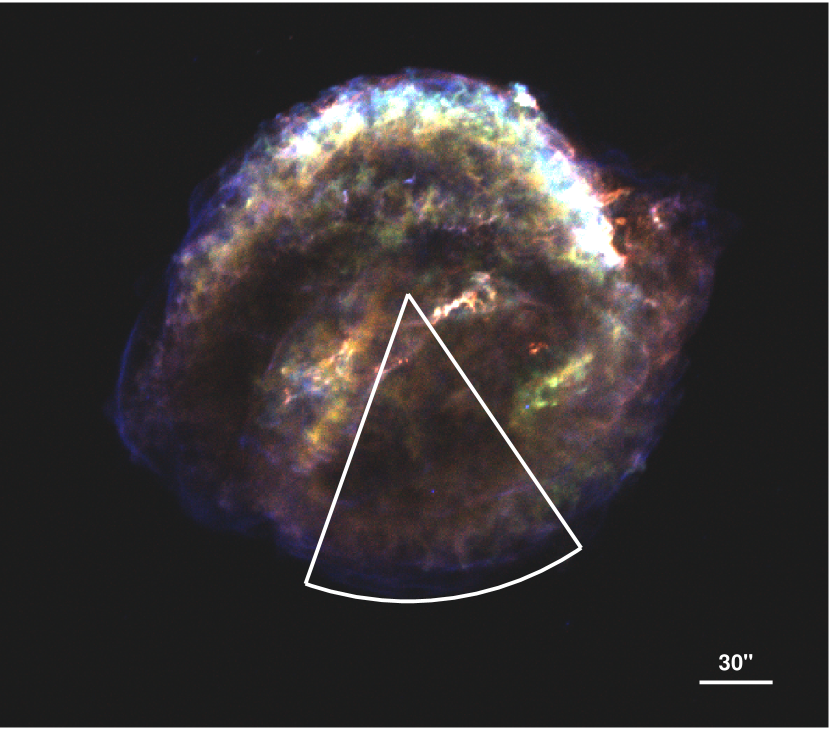
Figure 1.— Kepler’s SNR viewed in X-rays with Chandra ACIS-S3. The RGB image shows $0.4$–$0.75$ keV emission in red, $0.75$–$1.2$ keV emission in green, and $1.2$–$7.0$ keV emission in blue. In the image, north is up and east is to the left.

Figure 2.— Left: Chandra ACIS-S spectrum of the pie-sliced region of Kepler’s SNR shown in Figure 1. For reference, we mark the positions of several K$\alpha$ lines that are used in the analysis. Right: Spectral fit to the 1.7–7.0 keV spectrum of the pie-sliced region shown in Figure 1.The fit parameters are listed in Table 1, and the positions of the K$\alpha$ lines are also marked. In both figures, the data are unbinned (1024 PHA channels).

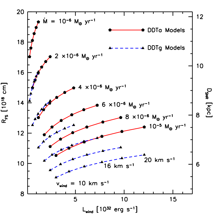
Figure 3.— Forward shock radius as a function of wind luminosity for a range of mass-loss rates and wind speeds, for Type Ia SN ejecta models DDTa and DDTg. On the right hand axis is the distance to Kepler that is implied by the forward shock radius, for an angular diameter of 4$\arcmin$, but the models may be scaled to any distance.

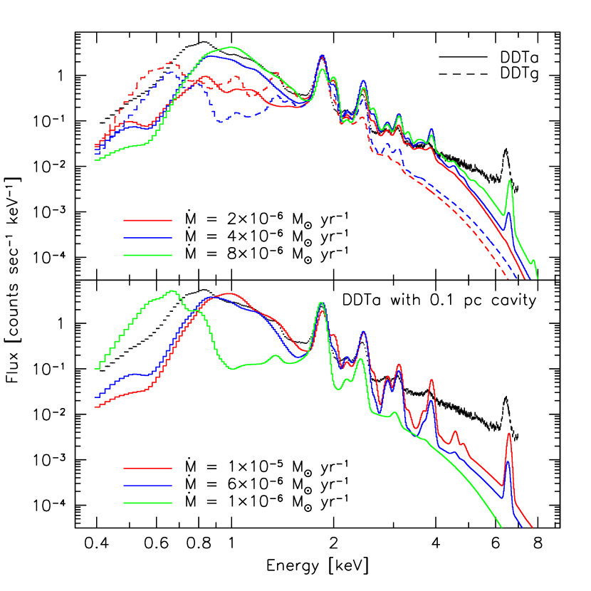
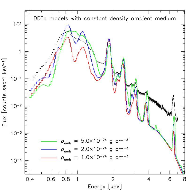
Figure 4.— Left: Comparisons between the modeled X-ray spectrum and the spectrum shown in Figure 1. In the upper panel, we compare the DDTa (solid lines) and DDTg (dashed lines) modeled spectra for a range of mass-loss rates, assuming a wind speed of 20 km s^-1. In the bottom panel, we plot the DDTa models for a wind speed of 20 km s^-1 and a range of mass-loss rates, assuming a small, low density cavity has formed around the progenitor. Right: DDTa models in a constant density ambient medium.

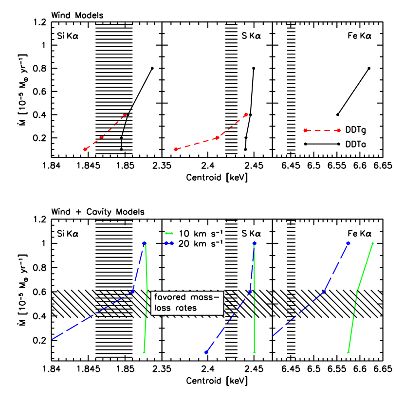
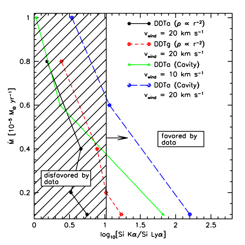
Figure 5.— Left: In the upper panel, we plot the measured versus computed line centroids for Si K$\alpha$, S K$\alpha$, and Fe K$\alpha$, for the DDTa (black solid) and DDTg (red dashed) models. The hatched region in each panel corresponds to the measured centroid including the 90% confidence interval The DDTg models and a subset of the DDTa models ($\dot{M}$ $<$ 4$\times$10^-6 M_☉ yr^-1) do not produce any Fe K emission. In the lower panel, we plot the line centroids for the DDTa cavity models for v_wind = 10 (green solid) and 20 (blue dashed) km s^-1, for a range of mass-loss rates. The line centroids and errors are indicated by the vertical hatched regions in each panel. The allowed mass-loss rates as dictated by the comparison between the measured and modeled line centroids are marked by the horizontal cross hatched region. Right: Si K$\alpha$/Si XIV Ly$\alpha$ flux ratio from each model as compared against the measured value from Table 1. The flux ratios are plotted as a function mass-loss rate for both the pure wind models as well as the models that include a cavity. The line styles are the same as in the left hand plot. We mark the region of the plot that is not consistent with the measured line ratio which rules out almost all pure wind models.

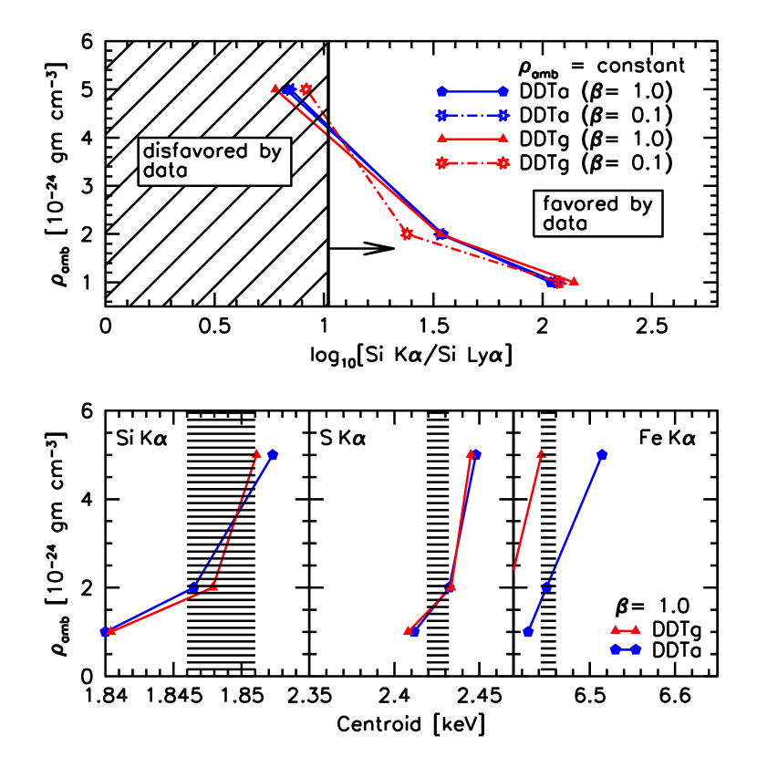
Figure 6.— Top: Si K$\alpha$/Si XIV Ly$\alpha$ flux ratio for energetic and subenergetic models in a constant density environment, for either instantaneous ($\beta$ = 1) or mass proportional ($\beta$ = 0.1) electron heating. The modeled ratio is relatively insensitive to the electron heating model. Bottom: Measured versus computed line centroids for the DDTa (blue) and DDTg (red) models for Si K$\alpha$, S K$\alpha$, and Fe K$\alpha$.

Table 1Spectral Parameters in Kepler’s SNR

Parameter	Fitted Value
Power-Law Continuum
$\alpha$	2.67${}^{+0.06}_{-0.01}$
Norm (10-3 photons cm-2 s-1 at 1 keV)	1.90${}^{+0.20}_{-0.02}$
Line Fluxes (10-5 photons cm-2 s-1)
Si K$\alpha$	49.9$\pm$0.20
Si XIV Ly$\alpha$	$<$ 4.70$\pm$0.47
Si K$\beta$	5.64$\pm$0.30
S K$\alpha$	13.5$\pm$0.30
Ar K$\alpha$	1.19$\pm$0.16
Ca K$\alpha$	0.38$\pm$0.07
Fe K$\alpha$	3.84$\pm$0.14
Line Centroids (keV)
Si K$\alpha$	1.848${}_{-0.002}^{+0.003}$
Si K$\beta$	2.190${}_{-0.003}^{+0.004}$
S K$\alpha$	2.425${}_{-0.006}^{+0.007}$
Ar K$\alpha$	3.077${}_{-0.006}^{+0.005}$
Ca K$\alpha$	3.799${}_{-0.010}^{+0.010}$
Fe K$\alpha$	6.450${}_{-0.008}^{+0.010}$
Line Width (eV)
Si K$\alpha$	25.9${}_{-1.0}^{+0.5}$
Si K$\beta$	62.2${}_{-3.2}^{+3.0}$
S K$\alpha$	35.9${}_{-1.0}^{+1.5}$
Ar K$\alpha$	36.0${}_{-5.5}^{+6.7}$
Ca K$\alpha$	57.9${}_{-12.0}^{+13.0}$
Fe K$\alpha$	83.0${}_{-5.1}^{+4.4}$

References

- Aharonian et al. (2008) Aharonian, F., et al. 2008, A&A, 488, 219
- Badenes et al. (2003) Badenes, C., Bravo, E., Borkowski, K. J., & Domínguez, I. 2003, ApJ, 593, 358
- Badenes et al. (2005) Badenes, C., Borkowski, K. J., & Bravo, E. 2005, ApJ, 624, 198
- Badenes et al. (2006) Badenes, C., Borkowski, K. J., Hughes, J. P., Hwang, U., & Bravo, E. 2006, ApJ, 645, 1373
- Badenes et al. (2007) Badenes, C., Hughes, J. P., Bravo, E., & Langer, N. 2007, ApJ, 662, 472
- Badenes et al. (2008) Badenes, C., Hughes, J. P., Cassam-Chenaï, G., & Bravo, E. 2008, ApJ, 680, 1149
- Bandiera (1987) Bandiera, R. 1987, ApJ, 319, 885
- Berezhko et al. (2006) Berezhko, E. G., Ksenofontov, L. T., & Völk, H. J. 2006, A&A, 452, 217
- Blair et al. (1991) Blair, W. P., Long, K. S., & Vancura, O. 1991, ApJ, 366, 484
- Blair et al. (2007) Blair, W. P., Ghavamian, P., Long, K. S., et al. 2007, ApJ, 662, 998
- Blondin & Lufkin (1993) Blondin, J. M., & Lufkin, E. A. 1993, ApJS, 88, 589
- Blondin et al. (2009) Blondin, S., Prieto, J. L., Patat, F., et al. 2009, ApJ, 693, 207
- Borkowski et al. (1992) Borkowski, K. J., Blondin, J. M., & Sarazin, C. L. 1992, ApJ, 400, 222
- Borkowski et al. (1994) Borkowski, K. J., Sarazin, C. L., & Blondin, J. M. 1994, ApJ, 429, 710
- Borkowski et al. (2009) Borkowski, K. J., Blondin, J. M., & Reynolds, S. P. 2009, ApJ, 699, L64
- Cassam-Chenaï et al. (2008) Cassam-Chenaï, G., Hughes, J. P., Reynoso, E. M., Badenes, C., & Moffett, D. 2008, ApJ, 680, 1180
- Castor et al. (1975) Castor, J., McCray, R., & Weaver, R. 1975, ApJ, 200, L107
- Castro et al. (2012) Castro, D., Slane, P. O., Ellison, D. C., & Patnaude, D. J. 2012, ApJsubmitted
- Chevalier (1982) Chevalier, R. A. 1982, ApJ, 258, 790
- Chiotellis et al. (2012) Chiotellis, A., Schure, K. M., & Vink, J. 2012, A&A, 537, A139
- Chomiuk et al. (2012) Chomiuk, L., Soderberg, A. M., Moe, M., et al. 2012, arXiv:1201.0994
- DeLaney et al. (2010) DeLaney, T., Rudnick, L., Stage, M. D., et al. 2010, ApJ, 725, 2038
- Drake et al. (2009) Drake, J. J., Laming, J. M., Ness, J.-U., et al. 2009, ApJ, 691, 418
- Dwarkadas & Chevalier (1998) Dwarkadas, V. V., & Chevalier, R. A. 1998, ApJ, 497, 807
- Garnavich et al. (1998) Garnavich, P. M., et al. 1998, ApJ, 509, 74
- Gerardy & Fesen (2001) Gerardy, C. L., & Fesen, R. A. 2001, AJ, 121, 2781
- Gomez et al. (2012) Gomez, H. L., Clark, C. J. R., Nozawa, T., et al. 2012, MNRAS, 2206
- Hachisu et al. (1996) Hachisu, I., Kato, M., & Nomoto, K. 1996, ApJ, 470, L97
- Howell et al. (2009) Howell, D. A., Conley, A., Della Valle, M., et al. 2009, arXiv:0903.1086
- Horesh et al. (2012) Horesh, A., Kulkarni, S. R., Fox, D. B., et al. 2012, ApJ, 746, 21
- Huang & Weigert (1982) Huang, R. Q., & Weigert, A. 1982, A&A, 116, 348
- Hwang & Laming (2012) Hwang, U., & Laming, J. M. 2012, ApJ, 746, 130
- Iben & Tutukov (1984) Iben, I., Jr., & Tutukov, A. V. 1984, ApJS, 54, 335
- Karakas & Lattanzio (2007) Karakas, A., & Lattanzio, J. C. 2007, PASA, 24, 103
- Li et al. (2011) Li, W., Bloom, J. S., Podsiadlowski, P., et al. 2011, Nature, 480, 348
- Lopez et al. (2011) Lopez, L. A., Ramirez-Ruiz, E., Huppenkothen, D., Badenes, C., & Pooley, D. A. 2011, ApJ, 732, 114
- Mazzali et al. (2007) Mazzali, P. A., Röpke, F. K., Benetti, S., & Hillebrandt, W. 2007, Science, 315, 825
- McKee & Ostriker (1977) McKee, C. F., & Ostriker, J. P. 1977, ApJ, 218, 148
- Milisavljevic et al. (2012) Milisavljevic, D., Fesen, R. A., Chevalier, R. A., et al. 2012, ApJ, 751, 25
- Nugent et al. (2011) Nugent, P. E., Sullivan, M., Cenko, S. B., et al. 2011, Nature, 480, 344
- Olofsson et al. (2002) Olofsson, H., González Delgado, D., Kerschbaum, F., & Schöier, F. L. 2002, A&A, 391, 1053
- Orlando et al. (2009) Orlando, S., Drake, J. J., & Laming, J. M. 2009, A&A, 493, 1049
- Owocki et al. (1994) Owocki, S. P., Cranmer, S. R., & Blondin, J. M. 1994, ApJ, 424, 887
- Park et al. (2007) Park, S., Slane, P. O., Hughes, J. P., et al. 2007, ApJ, 665, 1173
- Patat et al. (2007) Patat, F., Chandra, P., Chevalier, R., et al. 2007, Science, 317, 924
- Patnaude et al. (2009) Patnaude, D. J., Ellison, D. C., & Slane, P. 2009, ApJ, 696, 1956
- Patnaude et al. (2010) Patnaude, D. J., Slane, P., Raymond, J. C., & Ellison, D. C. 2010, ApJ, 725, 1476
- Perlmutter et al. (1998) Perlmutter, S., et al. 1998, Nature, 391, 51
- Perlmutter et al. (1999) Perlmutter, S., Aldering, G., Goldhaber, G., et al. 1999, ApJ, 517, 565
- Petruk (1999) Petruk, O. 1999, A&A, 346, 961
- Phillips et al. (1992) Phillips, M. M., Wells, L. A., Suntzeff, N. B., Hamuy, M., Leibundgut, B., Kirshner, R. P., & Foltz, C. B. 1992, AJ, 103, 1632
- Ramstedt et al. (2009) Ramstedt, S., Schöier, F. L., & Olofsson, H. 2009, A&A, 499, 515
- Reynolds et al. (2007) Reynolds, S. P., Borkowski, K. J., Hwang, U., Hughes, J. P., Badenes, C., Laming, J. M., & Blondin, J. M. 2007, ApJ, 668, L135
- Reynoso & Goss (1999) Reynoso, E. M., & Goss, W. M. 1999, AJ, 118, 926
- Riess et al. (1998) Riess, A. G., Filippenko, A. V., Challis, P., et al. 1998, AJ, 116, 1009
- Sankrit et al. (2005) Sankrit, R., Blair, W. P., Delaney, T., Rudnick, L., Harrus, I. M., & Ennis, J. A. 2005, Advances in Space Research, 35, 1027
- Schöier & Olofsson (2001) Schöier, F. L., & Olofsson, H. 2001, A&A, 368, 969
- Schure (2010) Schure, K. M. 2010, Ph.D. Thesis
- Simon et al. (2009) Simon, J. D., Gal-Yam, A., Gnat, O., et al. 2009, ApJ, 702, 1157
- Sokoloski et al. (2006) Sokoloski, J. L., Luna, G. J. M., Mukai, K., & Kenyon, S. J. 2006, Nature, 442, 276
- Stephenson & Green (2002) Stephenson, F. R., & Green, D. A. 2002, Historical supernovae and their remnants (Oxford: Clarendon)
- Sternberg et al. (2011) Sternberg, A., Gal-Yam, A., Simon, J. D., et al. 2011, Science, 333, 856
- Truelove & McKee (1999) Truelove, J. K., & McKee, C. F. 1999, ApJS, 120, 299
- Vink (2008) Vink, J. 2008, ApJ, 689, 231
- Warren et al. (2005) Warren, J. S., Hughes, J. P., Badenes, C., et al. 2005, ApJ, 634, 376
- Webbink (1984) Webbink, R. F. 1984, ApJ, 277, 355
- Weinberger & Kerber (1997) Weinberger, R., & Kerber, F. 1997, Science, 276, 1382
- Williams et al. (2011) Williams, B. J., Blair, W. P., Blondin, J. M., et al. 2011, ApJ, 741, 96
- Wood-Vasey & Sokoloski (2006) Wood-Vasey, W. M., & Sokoloski, J. L. 2006, ApJ, 645, L53