Asymptotics for Exponential Levy Processes and their Volatility Smile: Survey and New Results

Abstract.

Exponential Lévy processes can be used to model the evolution of various financial variables such as FX rates, stock prices, etc. Considerable efforts have been devoted to pricing derivatives written on underliers governed by such processes, and the corresponding implied volatility surfaces have been analyzed in some detail. In the non-asymptotic regimes, option prices are described by the Lewis-Lipton formula which allows one to represent them as Fourier integrals; the prices can be trivially expressed in terms of their implied volatility. Recently, attempts at calculating the asymptotic limits of the implied volatility have yielded several expressions for the short-time, long-time, and wing asymptotics. In order to study the volatility surface in required detail, in this paper we use the FX conventions and describe the implied volatility as a function of the Black-Scholes delta. Surprisingly, this convention is closely related to the resolution of singularities frequently used in algebraic geometry. In this framework, we survey the literature, reformulate some known facts regarding the asymptotic behavior of the implied volatility, and present several new results. We emphasize the role of fractional differentiation in studying the tempered stable exponential Levy processes and derive novel numerical methods based on judicial finite-difference approximations for fractional derivatives. We also briefly demonstrate how to extend our results in order to study important cases of local and stochastic volatility models, whose close relation to the Lévy process based models is particularly clear when the Lewis-Lipton formula is used. Our main conclusion is that studying asymptotic properties of the implied volatility, while theoretically exciting, is not always practically useful because the domain of validity of many asymptotic expressions is small.

1. Introduction

In the classical Black-Scholes-Merton (BSM) European option pricing model (see [22] and [93]), asset processes are assumed to be strictly diffusive in nature and characterized by a single (log-normal) volatility $\sigma$. In practice, no actual option market conforms with this framework, so to make the BSM formula work, practitioners are forced to make the volatility argument in this formula depend on option maturity $(\tau)$ and strike $(K)$. Indeed, it is common practice in virtually all option markets to maintain a strike- and maturity-dependent implied volatility surface, $\sigma_{imp}(t;\tau,K)$, such that a call option on an asset $F$ paying $(F(T)-K)^{+}$ at expiration time $T\geq t$ has a time $t$ undiscounted price $C(t;\tau,K)$ given by

(1.1) $$\frac{C(t;\tau,K)}{F(t)}=\Phi(d_{+})-e^{k}\Phi(d_{-}),$$

where $k\triangleq\ln(K/F(t))$, $\tau\triangleq T-t$, $\Phi(\cdot)$ is the cumulative Gaussian distribution function, and

(1.2) $$d_{\pm}=\frac{-k\pm\frac{1}{2}\sigma_{imp}(t;\tau,K)^{2}\tau}{\sigma_{imp}(t;\tau,K)\sqrt{\tau}}.$$

Here and below, as usual,

$$\left(x\right)^{\pm}=\pm\max\left(\pm x,0\right).$$

Note that our version of the BSM formula assumes that the asset price $F$ is a risk-neutral martingale, an assumption that is easily relaxed or, in any case, justified if we consider $F$ a forward process. At time $t$, the $t$-observable function $\sigma_{imp}(t;\tau,K)$ can be implied (with assistance of interpolation and extrapolation techniques) from quoted call option prices at multiple maturities and strikes. For later use, notice that the term

(1.3) $$\Delta=\Phi(d_{+}),$$

is known as the option’s (forward) delta.

Below we often use the time value of a call option defined as follows

(1.4) $$\delta C\left(t;\tau,K\right)=C(t;\tau,K)-\left(F\left(t\right)-K\right)^{+},$$

or, equivalently,

(1.5) $$\frac{\delta C(t;\tau,K)}{F(t)}=\Phi(d_{+})-e^{k}\Phi(d_{-})-\left(1-e^{k}\right)^{+}.$$

For future reference, it is convenient to introduce the following non-dimensional function $\mathsf{C}^{BS}\left(v,k\right)$ of the annualized variance $v$ and log-strike $k$:

(1.6) $$\mathsf{C}^{BS}\left(v,k\right)=\Phi\left(\mathsf{d}_{+}\right)-e^{k}\Phi\left(\mathsf{d}_{-}\right),$$

where $0<v<\infty$, $-\infty<k<\infty$, and,

$$\mathsf{d}_{\pm}=\frac{-k\pm\frac{1}{2}v}{\sqrt{v}}.$$

In the limiting cases we have

$$\mathsf{C}^{BS}\left(0,k\right)=\left(1-e^{k}\right)^{+},\ \ \ \ \ \mathsf{C}^{BS}\left(\infty,k\right)=1.$$

It is clear that

$$\frac{C(t;\tau,K)}{F(t)}=\mathsf{C}^{BS}\left(\sigma_{imp}(t;\tau,K)^{2}\tau,\ln\left(\frac{K}{F(t)}\right)\right).$$

In most real markets, the market implied volatility function $\sigma_{imp}(t;\tau,K)$ differs very significantly from a constant, and may have considerable slope and convexity as a function of $K$ for both very small and very large values of $\tau$. To understand and explain this phenomenon, several alternative models have been proposed in the literature. see, e.g., [94], [39], [59], [14], [4], [76] among others. Broadly speaking, the available approaches can be categorized as follows:

• Local volatility (LV) models, where the instantaneous volatility $\sigma$ of $F$ is a deterministic function of time and $F$.

• Stochastic volatility (SV) models, where $\sigma$ is a random variable, possibly correlated with $F$.

• Jump models, where the process for $F$ is assumed to be a purely discontinuous jump-process.

• Universal volatility (UV) models, where local volatility, stochastic volatility, and jump processes are combined.

Full-blown UV models are rarely used in practice, and instead markets tend to converge around a simpler model that ultimately becomes a de facto market standard. For instance, LV models are popular in the field of equity derivatives, and jump-free combinations of LV and SV (known as LSV, or local-stochastic volatility, models) are dominant in the FX options arena. Such usage of simplified models is, however, rarely motivated by empirical facts, but instead are done for practical reasons in recognition of the fact that models that combine LV, SV, and jumps are often highly complicated to calibrate and implement. One particularly thorny issue is the question of how precisely to mix LV, SV, and jumps, a problem that is made especially vexing by the fact that even a simple model like LV can, on its own, match essentially any arbitrage-free option volatility surface (see, e.g., [39]).

In UV models, there are several potential strategies for attacking the “mixing” problem. As LV, SV, and jumps give rise to different dynamic evolution of the volatility surface over time, one idea is to embed observations of the volatility dynamics into the model calibration problem (see, e.g., [6] for a discussion). A closely related approach is to incorporate market-observable exotic option prices that are sensitive to the evolution of volatility, e.g. variance options, barrier options, and similar; this approach is commonly used in FX markets to mix LV and SV into an LSV model. Yet another idea is to examine various extremes of the volatility surface (short maturity, long maturity, large strikes, small strikes) and attempt to understand which type of model feature (SV/LV/jumps) will control the asymptotic model behavior most strongly and most “naturally”. This information, in turn, could then be used to inspire the model building process. To give an example, consider that the convexity of $\sigma_{imp}(t;\tau,K)$ around $K=F(t)$ can often be observed to be substantially higher for small option maturities than for larger ones. A pure LV model would model this by letting the convexity (in $F$) of the local volatility function decay rapidly as a function of time. Such a model would, however, be highly non-stationary, an undesirable model feature that can be avoided by introducing jumps or (mean-reverting) stochastic volatility.

The idea of considering volatility function asymptotics is particularly attractive from an analytical perspective, as one can often work out simple closed-form expressions for these asymptotics, even for complex models. For SV, LV, and LSV models the procedure for generating such asymptotics is well-understood (see e.g. [58] for a survey of recent results), and the range of validity for the resulting expansions has been examined closely, generally with fairly satisfying results. Recently, similar attempts have been undertaken for jump processes, especially for processes in the so-called exponential Lévy class. More precisely, these models write

(1.7) $$F(t)=F(0)e^{X(t)},$$

where $X(t)$ is a Lévy process. In this setup, particular emphasis has been put on the small-time asymptotic of $C(t;\tau,K)$ for $\tau\rightarrow 0$ and $K$ fixed at some level different from $F(t)$, see for instance [70], [105], [46], [48] among many others. A typical result in this area of research is that

(1.8) $$\delta C\left(t;\tau,K\right)\sim\tau,\quad K\neq F(t),$$

where $\sim$ indicates the leading order term as $\tau\rightarrow 0$. For this relation to be true, the corresponding implied volatility must explode in the short-time limit. This line of research is closely related in studying small time asymptotics for the densities of Lévy processes, see, e.g., [67], [98], [107], [44], [45], [84], [18]. Small-time results for at-the-money (ATM) options where $K=F(t)$ are scarcer, but in [30] Tanaka’s formula is used to demonstrate that

(1.9) $$C\left(t;\tau,F(t)\right)\sim\left\{\begin{array}[]{cc}\tau,&\sigma=0,\\ \sqrt{\tau},&\sigma\neq 0,\end{array}\right.$$

when $X$ is a mixed jump-diffusion consisting of a Brownian motion with volatility $\sigma$ and a finite variation Lévy jump process. [116] further elaborates on this result in implied volatility space, and demonstrates that for a finite variation Lévy process (necessarily without a diffusion component)

(1.10) $$\sigma_{imp}\left(t;\tau,F(t)\right)\sim\sqrt{2\pi\tau}\max\left\{\int_{\mathbb{R}}\left(e^{x}-1\right)^{+}\nu\left(dx\right),\int_{\mathbb{R}}\left(1-e^{x}\right)^{+}\nu\left(dx\right)\right\},$$

where $\nu(\cdot)$ is the Lévy measure of $X.$ In the presence of a diffusion component with constant volatility $\sigma$, [116] shows that if

$$\int_{\mathbb{R}}x^{2}\nu(dx)<\infty,$$

then

$$\sigma_{imp}\left(t;\tau,F(t)\right)\sim\sigma$$

for $\tau\rightarrow 0$. Other relevant papers about short-time option prices in models with jumps include [2], [91], and [96].

As for long-maturity and extreme strike asymptotics, the literature is generally quite sparse. Under mild regularity conditions, [117], [103] use large deviation principles to demonstrate that the implied volatility surface will always flatten out for large enough maturities and finite strikes, irrespective of the underlying process assumptions, which agrees with earlier observations by [11]. For exponentiated Lévy processes, the authors list explicit formulas tying the long-time volatility asymptote to moments of $F$. Extreme strike asymptotics for the specific case of Lévy processes follow from the moment formulas of [69], [15], [16] and [55]; see [116] for a brief discussion.

Overall, while some progress has been made in recent years, the available asymptotic results for jump processes are limited when compared to the literature for LV and SV diffusion processes. In particular, little is known about the range of validity of jump process asymptotics, in part due to the difficulty of establishing accurate numerical option prices for Lévy processes, especially in the short-time limit. In this paper, we add to the literature in several ways. First and foremost, we completely characterize the $\tau$ and $K$ volatility surface asymptotes for the important class of (exponentiated) tempered stable Lévy processes, with and without a diffusive component. In addition, we also list a number of asymptotic expansions for the Merton jump-diffusion and the NIG (Normal Inverse Gaussian) process. Note that our results cover not only the level of the volatility surface, but also its slope and convexity – properties that are highly relevant when calibrating a model to observed option prices. We mainly work in Fourier space using the Lewis-Lipton call option representation [72], [76], and our primary tools for asymptotic expansion are the dominated convergence theorem (for the short-time limits) and classical complex variable techniques, such as the saddlepoint theorem (for long-dated options) and high-frequency Fourier asymptotics (for large and small strike limits). For testing and illustration purposes, we present several closed-form option prices for special cases of the tempered stable Lévy process, and also list some results for the computation of Green’s function. Further, we draw attention to the applicability of fractional differentiation in characterizing the PIDE (partial integro-differential equation) that governs option prices in the tempered stable model class; these results allows one to draw on modern numerical algorithms when pricing both vanilla and exotic options. As an example, we develop an operator splitting method which is $O\left(N^{2}\right)$ complex and second order accurate in time and space. The idea is to split jumps into positive and negative and treat them separately on each step; the problem then boils down to the inversion of Hessenberg matrices which may be accomplished via the generalized Thomas algorithm in $O\left(N^{2}\right)$ operations. A regular diffusion can be added as an additional iteration, as needed.

To test and motivate our asymptotic results, our primary focus in this paper is on FX options markets. These markets are of interest to us for two reasons: i) very short-dated options actively trade in this market (it is not uncommon for dealers to quote on options with a maturity being just a few hours); and ii) volatility quoting conventions in these markets use the option delta $\Delta$ (see (1.3)), rather than the strike $K$. At first glance the delta quotation standard may appear to be a nuisance, since additional translation from the delta space into the strike space is needed, but on second thought it becomes apparent that this construct has deep mathematical roots. Specifically, quoting volatility as a function of delta is closely related to the so-called resolution of singularities frequently used in algebraic geometry and other mathematical disciplines (see [9]). Our tests disprove a number of “urban myths” about Lévy process asymptotics, especially regarding the range of applicability of short- and long-time asymptotics.

Our paper is organized as follows. Section 2 provides a very brief introduction to FX volatility quotation standards, and introduce the concepts of risk reversals and straddles (also known as butterflies). We examine some representative market data for implied volatility, and highlight how the short-dated asymptotics are unnatural in a diffusion setting. Section 3 gives an overview of Lévy processes, with an emphasis on the tempered stable class and the fractional derivative representation of the corresponding option pricing equation. It also discusses both conventional and novel numerical methods for the tempered stable class which capitalize on their interpretation as fractional derivatives. Section 4 discusses some representative examples. Section 5 introduces the Lewis-Lipton formula which is the main working tool for establishing all our asymptotic results. It also discusses calibration of the corresponding stochastic processes to market data introduced in Section 2. Section 6 discusses the asymptotic behavior of the BSM formula which is used subsequently in order to analyze the behavior of implied volatility. Sections 7, 8 study long-time and short-time asymptotics, respectively, and Section 9 deals with wing asymptotics. Besides deriving theoretical results, Sections 7, 8, 9 also contain a series of numerical tests aimed at establishing their practical relevance. Finally, conclusions are drawn in Section 10. Appendices contain some of the more elaborate proofs and other useful material.

2. Background on FX Market

The FX options market is one of the largest over-the-counter options markets in the world, yet its conventions are quite idiosyncratic and differ markedly from those used in other derivatives markets (e.g., interest rates and equities). Moreover, almost every concept of importance can be interpreted differently, often depending on the currency pair in question, which makes systematic analysis and comparison of FX options particularly difficult. There are both historical and financial reasons for the existence of FX quotation styles, the most obvious being that FX transactions, unlike many other financial transactions, are inherently symmetric in nature, in the sense that units of currency are exchanged into units of currency (see, e.g., [75]).

In FX markets, it is standard practice to represent the volatility smile in terms of the option delta, rather than in terms of the option strike. We may define

(2.1) $$\Sigma(t;\tau,\Delta)=\sigma_{imp}\left(t;\tau,K\right)$$

where $\Delta$ is the delta defined in (1.3). The map between $\Delta$ and $K$ is monotonic, so (2.1) is always well-defined. We should note that several other definitions of delta than (1.3) exist in the FX market, not all of which are monotonic in strike; for our purposes, we ignore this complication and just refer to [102] and [33], among many other sources, for additional information on various delta definitions.

In the FX options markets, the function $\Sigma(t;\tau,\Delta)$ is normally liquidly quoted at only three different levels of delta: 0.25, 0.50, and 0.75. Somewhat confusingly, only $\Sigma(t;\tau,0.5)$ is directly quoted (the at-the-money volatility $\sigma_{ATM}$, where $K=F(t)$), whereas $\Sigma(t;\tau,0.25)$ and $\Sigma(t;\tau,0.75)$ must be constructed from quotes for risk-reversals (RRs) and butterflies (BFs) (also known as strangles). The relevant formulas are

$$\sigma_{ATM}(t;\tau) =\Sigma(t;\tau,0.5),$$

$$RR(t;\tau) =\Sigma(t;\tau,0.75)-\Sigma(t;\tau,0.25),$$

$$BF(t;\tau) =\frac{1}{2}\left(\Sigma(t;\tau,0.75)+\Sigma(t;\tau,0.25)-2\sigma_{ATM}(t;\tau)\right),$$

which trivially allows us to construct $\Sigma(t;\tau,0.75)$ and $\Sigma(t;\tau,0.25)$ from knowledge of $\sigma_{ATM}$, $RR$, and $BF$. It is clear that the RRs and BFs are closely related to the slope and convexity, respectively, of $\Sigma(t;\tau,\Delta)$ around $\Delta=0.5$. Specifically, we can write (omitting arguments)

(2.2) $$RR\approx\frac{1}{2}\frac{\partial\Sigma}{\partial\Delta};\quad BF\approx\frac{1}{32}\frac{\partial^{2}\Sigma}{\partial\Delta^{2}},$$

where the derivatives are evaluated around $\Delta=0.5$.

In Table 1 below, we show some sample market quotes for $\sigma_{ATM}\left(\tau\right)$, $RR\left(\tau\right)$, and $BF\left(\tau\right)$ for the USD/JPY currency pair. We highlight that the figure suggests the existence of non-zero finite limits for all three quotes $\sigma_{ATM},$ $RR$, and $BF$ as $\tau$ approaches zero. From (2.2), this essentially translates into non-zero finite limits for both $\partial\Sigma/\partial\Delta$ and $\partial^{2}\Sigma/\partial\Delta^{2}$ around the ATM point.

1d 1w 2w 1m 2m 3m 6m 1y 2y 3y 4y 5y ATM 9.87 12.15 11.27 10.35 10.34 10.52 11.04 11.80 12.90 13.80 14.30 15.05 RR25 -1.25 -1.00 -0.46 -0.30 -0.16 -0.10 -0.05 -0.02 -0.35 -0.78 -1.20 -1.48 BF25 0.30 0.30 0.30 0.30 0.32 0.33 0.46 0.59 0.60 0.58 0.53 0.46 RR10 -2.22 -1.77 -0.79 -0.49 -0.22 -0.09 0.07 0.18 -0.50 -1.41 -2.30 -2.86 BF10 1.11 1.08 1.03 1.02 1.08 1.12 1.54 1.98 2.11 2.22 2.28 2.29

Table 1. The behavior of $\sigma_{ATM}\left(\tau\right),$ $RR\left(\tau\right)$, and $BF\left(\tau\right)$ (expressed in per cent) for USD/JPY on March 30th, 2012. $RR25$ and $RR10$ are the risk-reversals at $\Delta=0.25$ and $\Delta=0.10$, respectively (and similar for $BF25$, $BF10$).

To understand the implications of Table 1 for the volatility smile in strike space, recall our definition of log-moneyness $k=\ln(K/F(t))$ and notice that

(2.3) $$\frac{\partial\Sigma}{\partial\Delta}=-\frac{\partial\sigma_{imp}}{\partial k}\sqrt{2\pi\tau},\quad\frac{\partial^{2}\Sigma}{\partial\Delta^{2}}=\left(\frac{\partial^{2}\sigma_{imp}}{\partial k^{2}}-\frac{1}{2}\frac{\partial\sigma_{imp}}{\partial k}\right)2\pi\tau,$$

where the derivatives are taken around $\Delta=0.5$ or, equivalently, $k=0$. To match non-zero limits of $\partial\Sigma/\partial\Delta$ and $\partial^{2}\Sigma/\partial\Delta^{2}$ for $\tau\rightarrow 0$, we evidently need both the smile skew $\partial\sigma_{imp}/\partial k$ and the smile convexity $\partial^{2}\sigma_{imp}/\partial k^{2}$ to approach infinity at $k=0$ for small $\tau$, at rates of $\tau^{-1/2}$ and $\tau^{-1}$, respectively. Such a requirement, however, would rule out that FX dynamics are driven by a pure diffusion process (such as LSV models), since it is known (see Section 8.3) that such processes always result in a finite limit of $\partial\sigma_{imp}/\partial k$ at $k=0$. Motivated by this observation, we proceed below to introduce the class of Lévy processes.

The data in Table 1 can be converted (with the aid of interpolation and extrapolation) into the function $\Sigma\left(\tau,\Delta\right)$. The result is shown in Figure 1. It is clear that the FX options exhibit strong smile for short and medium maturities.

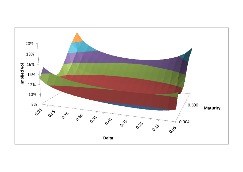
Figure 1. USDJPY implied volatility surface. The quotes are for March 30th, 2012.

3. Background on Exponential Lévy Processes

3.1. Basic Setup

In this section we consider exponential Lévy processes (ELPs). General properties of these processes are discussed in detail by numerous researchers, see, e.g., [21], [109], [8], among many others. The realization that these processes have important applications to finance can be traced back to [83] (and, in fact, to much earlier work); these applications are discussed in many books and papers, see, e.g., [41], [17], [101], [13], [24], [111], [7], [34], to mention just a few.

Let $X(t)$ be a Lévy process, i.e. a cadlag process with stationary and independent increments, satisfying $X(0)=0.$ It is known that every Lévy process is characterized by a triplet $(\bar{\gamma},\sigma,\nu)$, where $\bar{\gamma}$ and $\sigma$ are constants, and $\nu$ is a (possibly infinite) Radon measure, known as the Lévy measure. The Lévy measure must always satisfy

(3.1) $$\int_{\mathbb{R}}\min\left(x^{2},1\right)\nu(dx)<\infty.$$

To characterize the infinitesimal generator of a Lévy process, let $\mathrm{E}$ be the expectation operator, and define

$$V(t,x)=\mathrm{E}\left(V_{T}(X(T))|X(t)=x\right)$$

for some suitably regular function $V_{T}(\cdot)$. It can be shown that $V$ solves a partial integro-differential equation (PIDE) of the form

$$V_{t}+\bar{\gamma}V_{x}+\frac{1}{2}\sigma^{2}V_{xx}+\int_{\mathbb{R}}\left(V(t,x+y)-V\left(t,x\right)-y1_{|y|\leq 1}V_{x}\left(t,x\right)\right)\,\nu(dy)=0,$$

subject to the terminal condition $V\left(T,x\right)=V_{T}\left(x\right)$. More conveniently, we write this PIDE as

(3.2) $$V_{t}+\gamma V_{x}+\frac{1}{2}\sigma^{2}\left(V_{xx}-V_{x}\right)+\int_{\mathbb{R}}\left(V(t,x+y)-V\left(t,x\right)-y1_{|y|\leq 1}V_{x}\left(t,x\right)\right)\,\nu(dy)=0,$$

where $\gamma=\bar{\gamma}+\sigma^{2}/2$. Loosely speaking, (3.2) demonstrates that any Lévy process $X(t)$ is the sum of a deterministic drift term $\gamma t$, a scaled drift-adjusted Brownian motion $\sigma W(t)-\sigma^{2}t/2$, and a pure jump process.

By choosing $V_{T}\left(x\right)=\exp(iux)$ and solving (3.2) through an affine ansatz

$$V(t,x)=\exp(\psi(u)(T-t)+iux),$$

one arrives at the famous Lévy-Khinchine formula,

$$\phi(t,u)\triangleq\mathrm{E}\left(e^{iuX(t)}\right)=\exp\left(\psi(u)t\right),$$

(3.3) $$\psi(u)=\gamma iu-\frac{1}{2}\sigma^{2}u\left(u+i\right)+\int_{\mathbb{R}}\left(e^{iux}-1-iux1_{|x|\leq 1}\right)\,\nu(dx),\quad u\in\mathbb{R},$$

where $\psi$ is the so-called Lévy exponent. In practice, a Lévy process may be specified either by its exponent $\psi$ or by its Lévy measure $\nu$. It is frequently convenient to split $\psi(u)$ into two parts as follows

(3.4) $$\psi(u)=-\frac{1}{2}\sigma^{2}u(u+i)+\psi_{0}(u),$$

where $\psi_{0}(u)$ is the pure-jump and drift component of $\psi(u)$.

Let $F(t)>0$ denote the time $t$ price of a financial asset, and consider modeling its evolution as an exponential Lévy process of the type (1.7), where we wish for $F(t)$ to be a martingale in some pricing measure. For this, we impose that, for any $t>0$,

(3.5) $$\mathrm{E}\left(e^{X(t)}\right)=1,$$

which requires that the first exponential moment of $X(t)$ exists in the first place, i.e. that large positive jumps be suitably bounded:

(3.6) $$\int_{|x|>1}e^{x}\nu(dx)<\infty.$$

Equivalently, we require that $\phi(t,z)$ exists in the complex plane strip

$$\mathcal{S}=\{z\in\mathbb{C}|\mathrm{Im}(z)\in[-1,0]\},$$

and that

$$\phi(t,-i)=\exp\left(\gamma t+t\int_{\mathbb{R}}\left(e^{x}-1-x1_{|x|\leq 1}\right)\,\nu(dx)\right)=1,$$

in order to satisfy condition (3.5). This implies the fundamental martingale constraint

(3.7) $$\gamma=-\int_{\mathbb{R}}\left(e^{x}-1-x1_{|x|\leq 1}\right)\,\nu(dx).$$

Using (3.7) to eliminate $\gamma$ from (3.3), the martingale restriction on $F$ allows us to write the Lévy exponent in the form

(3.8) $$\psi(u)=-\frac{1}{2}\sigma^{2}u(u+i)+\int_{\mathbb{R}}\left(e^{iux}-1-iu\left(e^{x}-1\right)\right)\,\nu(dx).$$

Similarly, we may write the PIDE (3.2) as

(3.9) $$V_{t}+\frac{1}{2}\sigma^{2}\left(V_{xx}-V_{x}\right)+\int_{\mathbb{R}}\left(V(t,x+y)-V\left(t,x\right)-\left(e^{y}-1\right)V_{x}\left(t,x\right)\right)\,\nu(dy)=0.$$

Whenever possible (see Section 3.2), it is often more convenient to use the following forms of the PIDE (3.2), namely,

(3.10) $$V_{t}+\gamma^{\prime}V_{x}+\frac{1}{2}\sigma^{2}\left(V_{xx}-V_{x}\right)+\int_{-\infty}^{\infty}\left(V\left(t,x+y\right)-V\left(t,x\right)\right)\nu(dy)=0,$$

(3.11) $$V_{t}+\gamma^{\prime\prime}V_{x}+\frac{1}{2}\sigma^{2}\left(V_{xx}-V_{x}\right)+\int_{-\infty}^{\infty}\left(V\left(t,x+y\right)-V\left(t,x\right)-yV_{x}\left(t,x\right)\right)\nu(dy)=0,$$

where

(3.12) $$\gamma^{\prime}=-\int_{\mathbb{R}}\left(e^{x}-1\right)\,\nu(dx)=\gamma-\int_{|x|\leq 1}x\nu(dx),$$

(3.13) $$\gamma^{\prime\prime}=-\int_{\mathbb{R}}\left(e^{x}-1-x\right)\,\nu(dx)=\gamma+\int_{|x|>1}x\nu(dx).$$

3.2. Classification of Exponential Lévy Processes

Depending on how “singular” the Lévy measure $\nu$ is, we can define various sub-groups of Lévy processes. Each group allow us to decompose equations (3.3) and (3.2) in slightly different ways.

3.2.1. Finite Activity

First, if the Lévy measure is finite (i.e., the jump component of the process has finite activity), the resulting process for $X(t)$ is a combination of a Brownian motion and an ordinary compound Poisson jump-process. We may then replace $\nu(dx)$ with

(3.14) $$\nu(dy)=\lambda\,j(dy),\quad\lambda\triangleq\int_{\mathbb{R}}\nu(dx)<\infty,$$

where $j(dx)=\nu(dx)/\lambda$ is now a properly normed probability measure for the distribution of jump sizes in $X$, and $\lambda$ is the (Poisson) arrival intensity of jumps. In this case,

$$\psi(u)=\gamma^{\prime}iu-\frac{1}{2}\sigma^{2}u\left(u+i\right)+\lambda\left(\int_{\mathbb{R}}e^{iux}j(\,dx)-1\right),$$

where the martingale restriction requires that $\gamma^{\prime}$ satisfies (3.12). Notice that if we define a random variable $J$ with density $j(dx)$, then we can, in the finite activity case, interpret

(3.15) $$\psi(u)=\gamma^{\prime}iu-\frac{1}{2}\sigma^{2}u\left(u+i\right)+\lambda\left(\phi_{J}(u)-1\right),$$

where $\phi_{J}(\cdot)$ is the characteristic function of the jump size $J$.

As for the PIDE (3.2), for finite activity processes it simplifies in an analogous way to the simpler form (3.10):

$$V_{t}+\gamma^{\prime}V_{x}+\frac{1}{2}\sigma^{2}\left(V_{xx}-V_{x}\right)+\lambda\int_{\mathbb{R}}V(t,x+y)\,\,j(dy)-\lambda V=0.$$

3.2.2. Finite Variation

The jump component of a Lévy process is said to have finite variation if

(3.16) $$\int_{|x|\leq 1}|x|\nu(dx)<\infty.$$

Under this condition, truncation of the Lévy exponent $\psi$ around the origin is not necessary, and we may write

(3.17) $$\psi(u)=\gamma^{\prime}iu-\frac{1}{2}\sigma^{2}u\left(u+i\right)+\int_{\mathbb{R}}\left(e^{iux}-1\right)\nu(\,dx),\ \ \ \gamma^{\prime}=\gamma-\int_{|x|\leq 1}x\nu(dx).$$

For the PIDE (3.2), we then get the simpler form (3.10).

3.2.3. Finite First Moment

Finally, for the case where the first moment exists,

(3.18) $$\int_{\mathbb{R}}|x|1_{|x|>1}\nu(\,dx)<\infty,$$

we may write the Lévy exponent in purely compensated form:

$$\psi(u)=\gamma^{\prime\prime}iu-\frac{1}{2}\sigma^{2}u\left(u+i\right)+\int_{\mathbb{R}}\left(e^{iux}-1-iux\right)\nu(\,dx),\ \ \ \gamma^{\prime\prime}=\gamma+\int_{|x|>1}x\nu(dx).$$

The corresponding PIDE can then be written in the simpler form (3.11).

Going forward we shall often omit primes on $\gamma$ and simply use $\gamma$ to denote the drift term of the PIDE, implicitly choosing the right one.

4. Examples of Exponential Lévy Processes

4.1. Tempered Stable Processes

4.1.1. Definitions and Basic Facts

Establishing short-time ATM volatility smile asymptotics for the completely generic class of exponential Lévy processes appears to be a difficult problem, so we narrow our focus to classes of processes important in applications. Of primary importance to us are processes characterized by Lévy measures of the form

(4.1) $$\nu(dx)=\left(\frac{c_{+}}{x^{\alpha+1}}e^{-\kappa_{+}x}1_{x>0}+\frac{c_{-}}{|x|^{\alpha+1}}e^{-\kappa_{-}|x|}1_{x<0}\right)dx,$$

where we require that $\kappa_{+}\geq 1$, $\kappa_{-}\geq 0,$ $c_{+}\geq 0$, $c_{-}\geq 0$, and $\alpha<2.$ The resulting class of processes is known as tempered $\alpha$-stable Lévy processes (TSPs), see, e.g., [64], [89], [23], [24], [25], [34], [106]. Occasionally, a different parametrization of the Lévy measure is used

(4.2) $$\nu(dx)=-\frac{\sec\left(\frac{\alpha\pi}{2}\right)}{\Gamma(-\alpha)}\left(\frac{\vartheta_{+}^{\alpha}}{x^{\alpha+1}}e^{-\kappa_{+}x}1_{x>0}+\frac{\vartheta_{-}^{\alpha}}{|x|^{\alpha+1}}e^{-\kappa_{-}|x|}1_{x<0}\right)dx,$$

$\vartheta_{+}\geq 0$, $\vartheta_{-}\geq 0$, and $\sec\left(\pi/2\right)/\Gamma(-1)=-2/\pi$. This parametrization is particularly useful when one analyzes changes occurring when $\alpha$ crosses unity. Asymmetry of the TSP is often characterized by the non-dimensional number $\beta$,

(4.3) $$\beta=\frac{c_{+}-c_{-}}{c_{+}+c_{-}}.$$

It is clear that TSPs are natural extensions of the classical $\alpha$-stable Lévy processes (SPs), where $\kappa_{\pm}=0$, see, e.g., [122], [108], [97].

The overall behavior of the TS class is closely tied to the selection of the power $\alpha$, as demonstrated in Table 2.

$\alpha$ Activity Variation $<0$ Finite Finite $(0,1)$ Infinite Finite $[1,2)$ Infinite Infinite

Table 2. The behavior of the TS Lévy class as a function of $\alpha$.

Some important special cases of the TS class include:

• The KoBoL (CGMY) model, where $c_{+}=c_{-}$, see [64], [89], [23], [25];

• The exponential jump model, where $\alpha=-1$, see [65], [78];

• The Gamma process, where $\alpha=0$ and either $c_{-}=0$ or $c_{+}=0$;

• The Variance Gamma model, where $\alpha=0$, see [82];

• The Inverse Gaussian process, where $\alpha=1/2$ and either $c_{-}=0$ or $c_{+}=0$, see [12], [13].

For some of the special cases above, explicit formulas exist for the density of $X(t)$ and for European call options. Section 4.1.4 lists such formulas for the Inverse Gaussian process, which we use for testing various results later on.

When $\alpha\neq 0$ and $\alpha\neq 1,$ the characteristic function for the TS Lévy process can easily be shown to be, (see, e.g., [34],)

(4.4) $$\psi(u) =\sum\limits_{s=\pm}\Gamma\left(-\alpha\right)c_{s}\left(\left(\kappa_{s}-siu\right)^{\alpha}-iu\left(\kappa_{s}-s1\right)^{\alpha}+\left(iu-1\right)\kappa_{s}^{\alpha}\right)$$

$$=\sum_{s=\pm}a_{s}\left(\kappa_{s}-siu\right)^{\alpha}+\gamma iu+\delta,$$

where

(4.5) $$a_{s} =\Gamma\left(-\alpha\right)c_{s}=-\sec\left(\frac{\alpha\pi}{2}\right)\vartheta_{s}^{\alpha},\ \ \ \mathsf{\zeta}_{s}=\left(\kappa_{s}^{\alpha}-\left(\kappa_{s}-s\right)^{\alpha}\right),$$

$$\mathsf{\eta}_{s} =-\kappa_{s}^{\alpha},\ \ \ \gamma=a_{+}\mathsf{\zeta}_{+}+a_{-}\mathsf{\zeta}_{-},\ \ \ \delta=\left(a_{+}\mathsf{\eta}_{+}+a_{-}\mathsf{\eta}_{-}\right).$$

We have imposed the martingale condition (3.7) to express $\gamma$ as function of other parameters. In (4.4) the complex power functions

$$\left(\kappa_{+}-iu\right)^{\alpha},\ \ \ \left(\kappa_{-}+iu\right)^{\alpha},$$

are here (recall that $\alpha\neq 0,1,2)$ multi-valued functions, and an appropriate branch cut is required. We need, as a minimum, that $\psi(u)$ is regular for the strip$\ \mathcal{S}$, i.e. when $u=u^{\prime}+iu^{\prime\prime}$, $u^{\prime}\in\mathbb{R},$ $u^{\prime\prime}\in[-1,0]$. In this strip, the two power functions evaluate to

$$\left(\kappa_{+}+u^{\prime\prime}-iu^{\prime}\right)^{\alpha},\ \ \ \left(\kappa_{-}-u^{\prime\prime}+iu^{\prime}\right)^{\alpha}.$$

As the real part of the argument of the power function is strictly positive in $\mathcal{S}$, a branch cut in the left half-plane (e.g., the usual principal value branch cut for the logarithm) will therefore suffice.

Equation (4.4) holds only for $\alpha\neq 1$ and $\alpha\neq 0$ (and $\alpha<2$, of course). When $\alpha=0,$ we get

(4.6) $$\psi(u)=\sum_{s=\pm}c_{s}\left(\log\left(\frac{\kappa_{s}}{\kappa_{s}-siu}\right)-\log\left(\frac{\kappa_{s}}{\kappa_{s}-s}\right)iu\right).$$

Proceeding as above, we can easily show that the arguments to the $\log$-functions in this expression are entirely in the right half-plane when $\mathrm{Im}u\in[-1,0]$; the principal value of the logarithm will suffice. Finally, for the case $\alpha=1$, we have

$$\psi(u)=\sum_{s=\pm}c_{s}\left(\kappa_{s}-siu\right)\log\left(\frac{\kappa_{s}-siu}{\kappa_{s}}\right)-\left(\kappa_{s}-s\right)\log\left(\frac{\kappa_{s}-s}{\kappa_{s}}\right)iu.$$

Again, we may interpret $\log$ as the principal value of the logarithm.

By using (4.4) it is easy to show that the annualized standard deviation of a TSP has the form

(4.7) $$stdev\left(X\left(1\right)\right)=\left(\Gamma\left(2-\alpha\right)\left(\frac{c_{+}}{\kappa_{+}^{2-\alpha}}+\frac{c_{-}}{\kappa_{-}^{2-\alpha}}\right)\right)^{1/2}.$$

Equation (4.7) allows us to get an idea of the magnitude of the implied volatility of ATM options on TSPs.

4.1.2. PIDEs and their Fractional Derivative Interpretation

Consider now the TS Lévy class with an added Brownian motion with volatility $\sigma$. For $\alpha\in(0,1)$ the PIDE (3.10) applies, and has the form

(4.8) $$V_{t}+\gamma^{\prime}V_{x}+\frac{1}{2}\sigma^{2}\left(V_{xx}-V_{x}\right)+\sum\limits_{s=\pm}c_{s}\int_{0}^{\infty}\left(V\left(x+sy\right)-V\left(x\right)\right)\frac{e^{-\kappa_{s}y}dy}{y^{1+\alpha}}=0.$$

For $\alpha\in(1,2)$ the PIDE (3.11) can be used,

(4.9) $$V_{t}+\gamma^{\prime\prime}V_{x}+\frac{1}{2}\sigma^{2}\left(V_{xx}-V_{x}\right)+\sum\limits_{s=\pm}c_{s}\int_{0}^{\infty}\left(V\left(x+sy\right)-V\left(x\right)-syV_{x}\left(x\right)\right)\frac{e^{-\kappa_{s}y}dy}{y^{1+\alpha}}=0.$$

Interestingly, it is possible to rewrite both (4.8) and (4.9) in terms of so-called fractional derivatives (see, e.g., [95], [100] for a survey, and [122] for a connection to regular, non-tempered stable Lévy processes). The development of fractional derivatives originated in the nineteenth century with Riemann, Liouville and Marchaud among others (see, e.g., [85]), and traditionally starts with the well-known Riemann-Liouville formula which allows one to reduce the calculation of an $n$-fold integral to the calculation of a single convolution integral. This formula can be extended in a natural way for $\alpha$-fold integrals for any $\alpha>0$. Its extension for negative $\alpha$, which can be viewed as $\alpha$-fold differentiation, can be done in several different ways; we find that the so-called Caputo definition is the most convenient for our purposes. For integer values of $\alpha,$ the Caputo derivative coincides with the regular derivative of order $\alpha.$ For non-integer values of $\alpha$, consider first $\alpha\in\left(0,1\right)$, and define left ($s=-1$) and right ($s=1$) fractional derivatives of order $\alpha$ as follows

$$\mathfrak{D}_{s}^{\alpha}V\left(x\right)=\frac{\left(-s\right)^{\alpha}}{\Gamma\left(-\alpha\right)}\int_{0}^{\infty}\left(V\left(x+sy\right)-V\left(x\right)\right)\frac{dy}{y^{1+\alpha}},\ \ \ \ \ s=\pm.$$

Under some mild regularity assumptions we can perform integration by parts and write

$$\mathfrak{D}_{s}^{\alpha}V\left(x\right)=\frac{\left(-s\right)^{\alpha-1}}{\Gamma\left(1-\alpha\right)}\int_{0}^{\infty}\frac{dV\left(x+sy\right)}{dy}\frac{dy}{y^{\alpha}}.$$

For all non-integer values of $\alpha\in(1,\infty)$ we may then define

$$\mathfrak{D}_{s}^{\alpha}V\left(x\right)=\frac{\left(-s\right)^{\alpha-1-\left\lfloor\alpha\right\rfloor}}{\Gamma\left(1+\left\lfloor\alpha\right\rfloor-\alpha\right)}\int_{0}^{\infty}\frac{d^{\left\lfloor\alpha\right\rfloor+1}V\left(x+sy\right)}{dy^{\left\lfloor\alpha\right\rfloor+1}}\frac{dy}{y^{\alpha-\left\lfloor\alpha\right\rfloor}},$$

where $\left\lfloor\alpha\right\rfloor$ is the floor function, i.e., the largest integer such that $\left\lfloor\alpha\right\rfloor<\alpha$. Notice that in general $\mathfrak{D}_{+}^{\alpha}V\left(x\right)$ is complex-valued even when $V\left(x\right)$ is real-valued.

We emphasize that with this definition, irrespective of $s$,

$$\mathfrak{D}_{s}^{\alpha}e^{iux}=(iu)^{\alpha}e^{iux},$$

consistent with what one would expect from a generalization of a regular derivative.

Lemma 4.1.

For $\alpha\in(0,2)$, $\alpha\neq 1$, the PIDEs (4.8), (4.9) may be written

(4.10) $$V_{t}+\gamma V_{x}+\frac{1}{2}\sigma^{2}\left(V_{xx}-V_{x}\right)+\sum\limits_{s=\pm}\left(-s\right)^{\alpha}a_{s}e^{s\kappa_{s}x}\mathfrak{D}_{s}^{\alpha}\left(e^{-s\kappa_{s}x}V\right)+\delta V=0,$$

where $a_{s},\gamma,\delta$ are given by expression (4.5).

Proof.

See Appendix A.    

Corollary 4.2.

In particular, for non-tempered stable processes with $\kappa_{\pm}=0$, the corresponding PIDE has the form

$$V_{t}+\frac{1}{2}\sigma^{2}\left(V_{xx}-V_{x}\right)+\sum\limits_{s=\pm}\left(-s\right)^{\alpha}a_{s}\left(\mathfrak{D}_{s}^{\alpha}V-V_{x}\right)=0.$$

4.1.3. Numerical Methods Based on Fractional Derivatives

The advantage of restating the original pricing PIDEs as fractional differential equations is that we may lean on a large body of literature on numerical methods for such equations. These methods have been developed over the last twenty years due to the fact that fractional differential equations have numerous physical applications, especially to the so-called anomalous diffusions, see, e.g., [31], [112] among many others. In this section we present some extensions of these methods for our setting where both left $(s=-1)$ and right $(s=+1)$ derivatives must be considered simultaneously.

Before proceeding, let us remind the reader that an $N\times N$ matrix $\mathcal{H}$ such that $h_{ij}=0$ when $j\leq i-2$ ($h_{ij}=0$ when $j\geq i+2$) is called an upper (lower) Hessenberg matrix. Such a matrix can be viewed as a generalization of a tri-diagonal matrix. An equation of the form

(4.11) $$\mathcal{H}\vec{p}=\vec{q},$$

can be solved for the vector $\vec{p}$ via an appropriate extension of the Thomas algorithm for tri-diagonal matrices at the cost of $O\left(N^{2}\right)$ operations. The advantages of using Hessenberg structure of the problem are manyfold (see [114]), the most obvious being the ability to rely on highly parallelizable solvers. Hessenberg matrices naturally arise when one wants to solve pricing equations with fractional derivatives. When such derivatives are one-sided (or, equivalently, jumps are one-sided) we can naturally represent them via Hessenberg matrices on a grid by virtue of an appropriately discretized $\mathfrak{D}_{s}^{\alpha}$. When they are two-sided, we can split the problem into two and consider positive and negative jumps in turn at each step. Diffusion can be added as needed. The Grünwald-Letnikov formula is often used for discretizing fractional derivatives, see, e.g., [92], [38], [115]. However, it is more convenient to discretize $\mathfrak{D}_{s}^{\alpha}$ directly, see, e.g., [113] for a discretization scheme that guarantees that the resulting finite difference scheme is stable. In this discretization scheme, fractional derivatives $\mathfrak{D}_{s}^{\alpha}$ in (4.10) turn into Hessenberg matrices $\mathcal{H}_{s}^{\alpha}$; while the diffusion-advection term turns into a standard tri-diagonal matrix $\mathcal{D}$. In order to take full advantage of the nature of the matrices $\mathcal{H}_{s}^{\alpha},\mathcal{D}$, we solve a generic evolution equation of the form (4.10) by splitting a typical time step $t^{m+1}\rightarrow t^{m},$ $\vec{V}^{m+1}\rightarrow\vec{V}^{m}$ into three, $\vec{V}^{m+1}\rightarrow\vec{V}^{\ast}$, $\vec{V}^{\ast}\rightarrow\vec{V}^{\ast\ast}$, $\vec{V}^{\ast\ast}\rightarrow\vec{V}^{m}$ as follows:

$$\left(I-\frac{1}{2}\Delta t\mathcal{H}_{+}^{\alpha}\right)\vec{V}^{\ast} =\left(I+\frac{1}{2}\Delta t\mathcal{H}_{+}^{\alpha}\right)\vec{V}^{m+1},$$

$$\left(I-\frac{1}{2}\Delta t\mathcal{H}_{-}^{\alpha}\right)\vec{V}^{\ast\ast} =\left(I+\frac{1}{2}\Delta t\mathcal{H}_{-}^{\alpha}\right)\vec{V}^{\ast},$$

$$\left(I-\frac{1}{2}\Delta t\mathcal{D}\right)\vec{V}^{m} =\left(I+\frac{1}{2}\Delta t\mathcal{D}\right)\vec{V}^{\ast\ast}.$$

It is clear that at the first and second intermediate steps we have to solve a Hessenberg system of equations, while at the third step we need to solve a tri-diagonal system of equations. We illustrate the scheme by numerically constructing the probability density function (PDF) of a typical TSP in two different ways, namely by solving the corresponding PIDEs and by numerically calculating its integral representation. Our results are shown in Figure 2, and it is clear that our method reproduces the corresponding PDF very accurately.

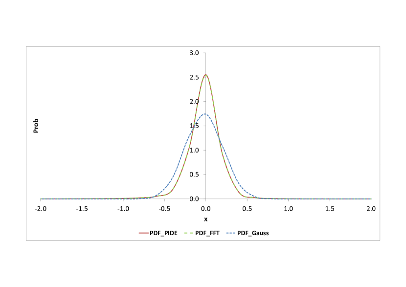
Figure 2. Numerical and analytical PDFs for a TSP. For comparison, PDFs for the moment-matched Gaussian process is shown as well, see (4.7). The corresponding parameters are $\alpha=1.50$, $\sigma=0.01\%$, $c_{+}=0.0069$, $c_{-}=0.0063$, $\kappa_{+}=1.9320$, $\kappa_{-}=0.4087$. The choice of parameters is justified in Section 5.5.

There are several well-known Fourier-transform-based and approximation-based approaches to solving the corresponding pricing equation in the spatially homogeneous case, see, e.g., [4], [10], [36], [32], [120], [60], [79], so, if this was the only case one is interested in, it would not be worthwhile adding yet another method to this set. However, to the best of our knowledge, none of these methods can be straightforwardly extended to the inhomogeneous case, nor to the case when barriers are present. Our method on the other hand can be extended to cover these cases almost verbatim.

4.1.4. Maximally Skewed Stable Processes

If we set $\kappa_{+}=\kappa_{-}=0$, the Lévy measure (4.1) becomes that of a regular stable process. This type of process has limited applications in finance, as we only can satisfy the martingale restriction (3.5) if we mandate that $c_{+}=0$ ($\beta=-1$, where $\beta$ is given by (4.3)), i.e. when all jumps are negative. The resulting process is sometimes known as the maximally negatively skewed stable process, and has received some interest in the literature, see [29]. The characteristic exponent for such processes is known in closed form. Using parametrization (4.2) and assuming that the process is a martingale, $\psi(u)$ can be defined as follows

(4.12) $$\psi(u)=\left\{\begin{array}[]{cc}\vartheta^{\alpha}\sec\left(\alpha\pi/2\right)\left(iu-(iu)^{\alpha}\right),&\alpha\neq 1,\\ \frac{2}{\pi}\vartheta iu\ln(iu),&\alpha=1,\end{array}\right.$$

in the complex strip $\mathcal{S}$ defined by $\mathrm{Im}\left(u\right)\in[-1,0]$. Despite the fact that jumps can only “go down” when $\beta=-1$, the already present drift-correction around the origin in the Lévy-Khinchine theorem makes the resulting process a martingale for $\alpha=1$, so no additional drift correction is necessary.

Remark 4.1.

There are three classical cases when the PDF for the stable Lévy process can be calculated explicitly: i) $\alpha=1/2,\beta=\pm 1$ (Lévy distribution); ii) $\alpha=1,\beta=0$ (Cauchy distribution); iii) $\alpha=2,1\leq\beta\leq 1$ (Gaussian distribution). Of these three cases, for option pricing purposes the only nontrivial case is $\alpha=1/2$ and $\beta=-1$, where

$$\nu(dx)=\frac{\sqrt{2\vartheta}}{2\sqrt{\pi}\left(-x\right)^{3/2}}\mathbf{1}_{x<0}dx.$$

Here, the distribution of $X(t)$ is

(4.13) $$\mathrm{P}\left(X(t)\in[x,x+dx]\right)=\frac{\iota}{2\sqrt{\pi}}\frac{\exp\left(-\frac{\iota^{2}}{4(\iota-x)}\right)}{\left(\iota-x\right)^{3/2}}\mathbf{1}_{x<\iota}dx,$$

where $\iota=\sqrt{2\vartheta}t$ and condition (3.5) is clearly satisfied, so that $\exp(X(t))$ is a martingale. Notice that in this case $X(t)$ is bounded from above by $\iota$, which may not be particularly realistic. Still, for testing purposes it is worthwhile developing this case further, so Proposition 4.3 develops an analytic call option formula for this model.

In order to avoid possible confusion, we call the maximally skewed Lévy process with $\alpha=1/2,\beta=\pm 1$, the Lévy-Gauss Process (LGP). By doing so we emphasize the so-called duality relation between the Lévy process with $\alpha=1/2,\beta=\pm 1$, and the standard Gaussian process with $\alpha=2$, see, e.g., [122].

Maximally skewed stable processes possess are scaling invariant, which allows one to write their Green’s functions in a simple form. Interestingly, a maximally skewed tempered stable process ($c_{+}=0$ and $\kappa_{-}>0$) can be transformed into a maximally skewed stable process ($c_{+}=0$ and $\kappa_{-}=0$). This result, which is listed in Appendix B, allows us to represent the Green’s function for maximally skewed tempered stable process in closed form. It also allows us to derive closed-form call option prices for certain TSPs, which shall be useful later on for testing purposes. For instance, we have:

Proposition 4.3.

Consider the price of a $T$-maturity, $K$-strike call option in an exponential tempered Lévy-Gauss process with $\alpha=1/2$ and $c_{+}=0$. Set $\iota=\sqrt{2\vartheta}\tau$, $\iota_{1}=\sqrt{\kappa_{-}}\iota$, $\iota_{2}=\sqrt{\kappa_{-}+1}\iota$, and $k=\ln(K/F(t))$. Further, assume that $k<\iota_{2}-\iota_{1}$, and set

$$v=\frac{2\iota^{2}}{\left(\iota_{2}-\iota_{1}-k\right)}.$$

We then have

(4.14) $$\frac{C\left(t;T,K\right)}{F(t)} =\mathsf{C}^{GL}\left(\tau,k\right),$$

$$\mathsf{C}^{GL}\left(\tau,k\right) =e^{\iota_{2}}\mathsf{D}\left(v,2\iota_{2}\right)-e^{k+\iota_{1}}\mathsf{D}\left(v,2\iota_{1}\right),$$

where $\mathsf{D}\left(v,k\right)$ is the symmetrized version of the Black-Scholes price given by

(4.15) $$\mathsf{D}\left(v,k\right)=e^{-\frac{k}{2}}\left(1-\mathsf{C}^{BS}\left(v,k\right)\right)=e^{-\frac{k}{2}}\Phi\left(-d_{+}\right)+e^{\frac{k}{2}}\Phi\left(d_{-}\right).$$

Proof.

See Appendix B.    

Similar formulas, albeit in a somewhat different context are given in [54].

Remark 4.2.

When $\alpha=1/2$, $c_{+}=0$, the price process $F(T)$ is always bounded from above by

$$F_{\max}\left(t,T\right)=F(t)e^{\iota_{2}-\iota_{1}}.$$

A similar bound exists for all $\alpha<1$. Paradoxically, when $\alpha\geq 1$ and $c_{+}=0$, $F(T)$ can take any value in $(0,\infty)$, despite all jumps being strictly negative.

4.2. Normal Inverse Gaussian Processes

As we have seen earlier, in some cases Lévy processes (such as a tempered Lévy-Gauss process) are localized on a semi-axis. Processes of that nature can be used in order to create new interesting processes by changing time for the regular Brownian motion. Below we discuss some examples along these lines. A useful aspect of this approach is that it generates Lévy processes with PDFs known in closed form. One of the well-known examples is the so-called Variance Gamma process (VGP), which is a special case of a TSP with $\alpha=0$, see, e.g., [82]. Another popular choice is the so-called Normal Inverse Gaussian process (NIGP), see, e.g., [12], [42], which we consider in some detail.

The Inverse Gaussian (IG) process describes the density of the hitting time $\tau$ of a level $\mathcal{\varkappa}_{1}t$ by a standard Brownian motion with volatility $\sigma_{1}$ and drift $\varkappa_{1}$. Our choice of parameters ensures that $\mathbb{E}\left(\tau\right)=t$. It is easy to verify that IGP as a TSP with $\alpha=1/2$, $\beta=1$, $\kappa_{+}=\varkappa_{1}^{2}/2\sigma_{1}^{2}$. It is clear that IGPs and TLGPs are closely related and can be transformed into each other via shift and reflection. IG process can be used as a subordinator in order to build the NIGP out of a standard Brownian motion.

The NIGP can be obtained by time changing of a standard Brownian motion with volatility $\sigma$ and drift $-\sigma^{2}/2$. The drift is chosen in a way ensuring that the corresponding NIG is a martingale. The corresponding subordinator is distributed as a hitting time of a level $\mathcal{\varkappa}_{1}t$ by an independent BM with volatility $\sigma_{1}$ and drift $\mathcal{\varkappa}_{1}$. The convolution of these two processes yields

(4.16) $$f^{NIG}\left(t,x\right)=\frac{\bar{\omega}\mathcal{\bar{\varkappa}}\sigma^{2}te^{-\frac{x}{2}+\mathcal{\bar{\varkappa}}^{2}\sigma^{2}t}}{\pi\sqrt{x^{2}+\mathcal{\bar{\varkappa}}^{2}\sigma^{4}t^{2}}}K_{1}\left(\bar{\omega}\sqrt{x^{2}+\mathcal{\bar{\varkappa}}^{2}\sigma^{4}t^{2}}\right),$$

where $K_{1}\left(.\right)$ is the modified Bessel function, and $\bar{\omega}=\sqrt{\mathcal{\bar{\varkappa}}^{2}+1/4}$, $\mathcal{\bar{\varkappa}=\varkappa}_{1}/\sigma_{1}\sigma$. The corresponding Lévy exponent and density have the form

$$\psi^{NIG}\left(u\right) =\sigma^{2}\mathcal{\bar{\varkappa}}\left(\mathcal{\bar{\varkappa}}-\sqrt{\mathcal{\bar{\varkappa}}^{2}+u\left(u+i\right)}\right),$$

$$\nu^{NIG}\left(dx\right) =\left(\lim_{t\rightarrow 0}\frac{f\left(t,x\right)}{t}\right)dx=\frac{\sigma^{2}\bar{\omega}\mathcal{\bar{\varkappa}}e^{-\frac{x}{2}}}{\pi\left|x\right|}K_{1}\left(\bar{\omega}\left|x\right|\right)dx,\ \ \ \ \ x\neq 0.$$

Although NIGPs are not a special case of TSPs, they are closely related to TSPs with $\alpha=1/2$ and $\alpha=1$, due to the fact that

$$K_{1}\left(\bar{\omega}\left|x\right|\right)\underset{\left|x\right|\rightarrow 0}{\sim}\frac{1}{\bar{\omega}\left|x\right|},\ \ \ K_{1}\left(\bar{\omega}\left|x\right|\right)\underset{\left|x\right|\rightarrow\infty}{\sim}\sqrt{\frac{\pi}{2\bar{\omega}\left|x\right|}}\left(1+\frac{3}{8\bar{\omega}\left|x\right|}\right)e^{-\bar{\omega}\left|x\right|},$$

so that

$$\nu^{NIG}\left(dx\right)\underset{\left|x\right|\rightarrow 0}{\sim}\frac{\sigma^{2}\mathcal{\bar{\varkappa}}e^{-\frac{x}{2}}}{\pi\left|x\right|^{2}},\ \ \ \ \ \nu^{NIG}\left(dx\right)\underset{\left|x\right|\rightarrow\infty}{\sim}\frac{\sigma^{2}\sqrt{\bar{\omega}}\mathcal{\bar{\varkappa}}}{\sqrt{2\pi}\left|x\right|^{3/2}}e^{-\left(\frac{x}{2}+\bar{\omega}\left|x\right|\right)}.$$

In the spirit of formula (1.6), the price of a call option with log-strike $k$ can be written in the form

(4.17) $$\frac{C^{NIG}\left(t;T,K;\sigma,\mathcal{\varkappa}_{1},\sigma_{1}\right)}{F(t)}=\mathsf{C}^{NIG}\left(v,k;\mathcal{\bar{\varkappa}}\right),$$

where, as usual, $v=\sigma^{2}\tau$, and

(4.18) $$\mathsf{C}^{NIG}\left(v,k;\mathcal{\bar{\varkappa}}\right)=\frac{\bar{\omega}\mathcal{\bar{\varkappa}}ve^{\mathcal{\bar{\varkappa}}^{2}v}}{\pi}\mathop{\displaystyle\int}\limits_{k}^{\infty}\frac{\left(e^{\frac{x}{2}}-e^{k-\frac{x}{2}}\right)}{\sqrt{x^{2}+\mathcal{\bar{\varkappa}}^{2}v^{2}}}K_{1}\left(\bar{\omega}\sqrt{x^{2}+\mathcal{\bar{\varkappa}}^{2}v^{2}}\right)dx.$$

Clearly, the normalized call price for a NIGP $\mathsf{C}^{NIG}$ depends on one non-dimensional parameter. (Recall that $\mathsf{C}^{BS}$ does not depend on any parameters.) In Section 5 we derive an alternative integral representation for $\mathsf{C}^{NIG}$, given by the Lewis-Lipton formula. We use one or the other of these two expressions as convenient.

As before, it is easy to compute the annualized standard deviation of a NIGP. The corresponding expression has the form

(4.19) $$stdev\left(X\left(1\right)\right)=\frac{\bar{\omega}\sigma}{\mathcal{\bar{\varkappa}}}.$$

Remark 4.3.

We note in passing that the so-called Generalized Inverse Gaussian (GIG) processes can be viewed as a natural generalizations of IGPs. In general, the density of such a process is not known analytically, while its Lévy density is given by a fairly complicated expression, so that GIG process is not easy (or necessary) to use in practice. It is not in the TSP class in any case.

4.3. Merton Processes

One popular process that is not related to the tempered stable class is the (pure-jump) Merton process (MP), with

$$\nu^{M}(dx)=\frac{\lambda}{\sqrt{2\pi}\eta}e^{-\frac{(x-\mu)^{2}}{2\eta^{2}}}dx.$$

This process has finite activity, so we may use (3.15) to establish $\psi(u)$. We get

$$\int_{\mathbb{R}}\left[e^{iux}-1\right]\nu(dx)=\lambda\left(e^{iu\mu-\frac{1}{2}\eta^{2}u^{2}}-1\right),$$

so, for a pure-jump MP,

(4.20) $$\psi(u)=\lambda\left(e^{iu\mu-\frac{1}{2}\eta^{2}u^{2}}-1\right)+\lambda\left(1-e^{\mu+\frac{1}{2}\eta^{2}}\right)iu=\lambda\left(e^{iu\mu-\frac{1}{2}\eta^{2}u^{2}}-1\right)+\gamma iu,$$

where $\gamma=\lambda\left(1-e^{q}\right),\ \ \ q=\mu+\frac{1}{2}\eta^{2}$. The corresponding PDF can be calculated explicitly,

$$f\left(t,x\right) =e^{-\lambda t}\sum_{n=0}^{\infty}\frac{\left(\lambda t\right)^{n}}{n!}f_{n}\left(t,x\right),$$

$$f_{n}\left(t,x\right) =\left\{\begin{array}[]{cc}\delta\left(x-\gamma t\right),&n=0,\\ \frac{1}{\sqrt{2\pi n}\eta}e^{-\frac{(x-\gamma t-n\mu)^{2}}{2n\eta^{2}}},&n>0,\end{array}\right.$$

It can be shown easily that

$$\nu^{M}\left(dx\right)=\left(\lim_{t\rightarrow 0}\frac{f\left(t,x\right)}{t}\right)dx=\lambda f_{1}\left(0,x\right)=\frac{1}{\sqrt{2\pi}\eta}e^{-\frac{(x-\mu)^{2}}{2\eta^{2}}},\ \ \ x\neq 0.$$

A simple calculation yields the following expression from [94] for the price of a call option

(4.21) $$\frac{C^{M}\left(t;T,K;\lambda,\mu,\eta\right)}{F(t)} =\mathsf{C}^{M}\left(v,k;\lambda,\mu,\eta\right),$$

$$\mathsf{C}^{M}\left(v,k;\mu,\eta\right) =\sum_{n=0}^{\infty}c_{n}\mathsf{C}^{BS}\left(n\eta^{2},l-nq\right),$$

where

$$c_{n}=e^{-e^{q}v}\left(e^{q}v\right)^{n}/n!,\ \ \ \ \ l=k-\left(1-e^{q}\right)v,\ \ \ \ \ v=\lambda\tau.$$

Analysis of MPs with diffusion component is very similar to the one performed above. The corresponding characteristic function has the form

$$\psi(u)=-\frac{1}{2}\sigma^{2}u\left(u+i\right)+\lambda\left(e^{iu\mu-\frac{1}{2}\eta^{2}u^{2}}-1\right)+\gamma iu,$$

while the price of a call option can be written as follows

$$\frac{C^{M}\left(t;T,K;\lambda,\mu,\eta\right)}{F(t)} =\mathsf{C}^{M}\left(v,k;\hat{\sigma},\mu,\eta\right),$$

$$\mathsf{C}^{M}\left(v,k;\hat{\sigma},\mu,\eta\right) =\sum_{n=0}^{\infty}c_{n}\mathsf{C}^{BS}\left(\hat{\sigma}^{2}v+n\eta^{2},l-nq\right),$$

where $c_{n},l$ have the same form as before, and $\hat{\sigma}=\sigma/\sqrt{\lambda}$.

The annualized standard deviation of a MP has the form

(4.22) $$stdev\left(X\left(1\right)\right)=\left(\sigma^{2}+\lambda\left(\mu^{2}+\eta^{2}\right)\right)^{1/2}.$$

Once again, this formula allows us to get a rough estimate of the magnitude of the implied volatility of ATM options on MPs.

5. The Lewis-Lipton Option Price Formula and its Implications

5.1. Exponential Lévy Processes

The key formula allowing one to analyze option prices for Lévy processes is known as the Lewis-Lipton (LL) formula; it has been independently proposed by Lewis [72] and Lipton [76]. This formula is based on the Fourier transform of an appropriately modified payoff of the call option. A complementary method is proposed in [27]; additional information can be found in [68].

Proposition 5.1.

The normalized price of a call option written on an underlying driven by an exponential Lévy process with Lévy-Khinchine exponent $\psi$ has the form

(5.1) $$\mathsf{C}\left(\tau,k\right)=1-\frac{1}{2\pi}\int_{-\infty}^{\infty}\frac{E\left(\tau,u\right)}{Q\left(u\right)}e^{-k\left(iu-\frac{1}{2}\right)}du.$$

Here

(5.2) $$E\left(\tau,u\right)=\exp\left(\tau\upsilon\left(u\right)\right)=\exp\left(\tau\left(\upsilon_{0}\left(u\right)-\frac{1}{2}\sigma^{2}Q\left(u\right)\right)\right),$$

(5.3) $$\upsilon\left(u\right)=\psi\left(u-\frac{i}{2}\right),\ \ \ \ \ \upsilon_{0}\left(u\right)=\psi_{0}\left(u-\frac{i}{2}\right),\ \ \ \ \ Q\left(u\right)=u^{2}+\frac{1}{4}.$$

and $\psi_{0}$ is given by (3.4).

Proof.

See [71], [72], [75], [76].    

As a corollary, we have:

Corollary 5.2.

The derivatives with respect to $k$ of the normalized price of a call option are

(5.4) $$\mathsf{C}_{k}\left(\tau,k\right) =-\frac{1}{2\pi}\int_{-\infty}^{\infty}\frac{E\left(\tau,u\right)}{Q\left(u\right)}e^{-k\left(iu-\frac{1}{2}\right)}\left(-iu+\frac{1}{2}\right)du,$$

(5.5) $$\mathsf{C}_{kk}\left(\tau,k\right) =-\frac{1}{2\pi}\int_{-\infty}^{\infty}\frac{E\left(\tau,u\right)}{Q\left(u\right)}e^{-k\left(iu-\frac{1}{2}\right)}\left(-iu+\frac{1}{2}\right)^{2}du.$$

Applying this result to the processes introduced in Section 4 we easily get the following lemma.

Lemma 5.3.

For TSPs, NIGPs, and MPs, the corresponding $E\left(\tau,u\right)$ have the form

$$E^{TS}\left(\tau,u\right) =\exp\left(\tau\left(-\frac{1}{2}\sigma^{2}Q\left(u\right)+\sum_{s=\pm}a_{s}\left(\kappa_{s}-s\left(iu+\frac{1}{2}\right)\right)^{\alpha}+\gamma\left(iu+\frac{1}{2}\right)+\delta\right)\right),$$

$$E^{NIG}\left(\tau,u\right) =\exp\left(\tau\sigma^{2}\mathcal{\bar{\varkappa}}\left(\mathcal{\bar{\varkappa}}-\sqrt{\mathcal{\bar{\omega}}^{2}+u^{2}}\right)\right),$$

$$E^{M}\left(\tau,u\right) =\exp\left(\tau\left(-\frac{1}{2}\sigma^{2}Q\left(u\right)+\lambda\left(e^{q\left(iu+\frac{1}{2}\right)-\frac{\eta^{2}}{2}Q\left(u\right)}-1+\left(1-e^{q}\right)\left(iu+\frac{1}{2}\right)\right)\right)\right).$$

Remark 5.1.

It is worth mentioning that $E^{TS}\left(\tau,u\right)$ and $E^{NIG}\left(\tau,u\right)$ rapidly decay when $\left|u\right|\rightarrow\infty$, so that computation of the integrals (5.1), (5.4), and (5.5) is straightforward. When $\sigma\neq 0$, $\ E^{M}\left(\tau,u\right)$ is rapidly decaying as well. However, when $\sigma=0$, the situation is more difficult. The corresponding integrals (5.1), (5.4) for this case can be computed efficiently by using

$$\frac{E^{M,\infty}\left(\tau,u\right)}{Q\left(u\right)}=\frac{\exp\left(\lambda\tau\left(-1+\left(1-e^{q}\right)\left(iu+\frac{1}{2}\right)\right)\right)}{Q\left(u\right)},$$

as a control variate.

Remark 5.2.

In the case of a BSM diffusion process, (5.1) yields

$$\mathsf{C}^{BS}\left(v,k\right)=1-\frac{1}{2\pi}\int_{-\infty}^{\infty}\frac{e^{-\frac{1}{2}vQ\left(u\right)-k\left(iu-\frac{1}{2}\right)}}{Q\left(u\right)}du,$$

so that

(5.6) $$\frac{1}{2\pi}\int_{-\infty}^{\infty}\frac{e^{-\frac{1}{2}vQ\left(u\right)-k\left(iu-\frac{1}{2}\right)}}{Q\left(u\right)}du=\Phi\left(\frac{k}{\sqrt{v}}-\frac{1}{2}\sqrt{v}\right)+e^{k}\Phi\left(-\frac{k}{\sqrt{v}}-\frac{1}{2}\sqrt{v}\right).$$

In the limiting case $v=0$, we get

(5.7) $$\frac{1}{2\pi}\int_{-\infty}^{\infty}\frac{e^{-k\left(iu-\frac{1}{2}\right)}}{Q\left(u\right)}du=e^{k^{-}}.$$

These useful formulas shall be used repeatedly in what follows.

The usefulness of the LL formula becomes apparent when one wants to study the asymptotic behavior of the call price and its derivatives (the Greeks) in the limiting cases of $\tau\rightarrow 0$, $\tau\rightarrow\infty$, $\left|k\right|\rightarrow\infty$, since it allows one to use enormous body of work dedicated to the asymptotics of integrals depending on large and small parameters. This is done in the remainder of the paper where it is shown how to apply the saddlepoint method, the high frequency Fourier integrals estimates, and other tricks to the problem at hand. We return to these asymptotics in Sections 7, 8, 9. While this is not the focus of this paper, the LL formula can also be used to study the small jump asymptotics, as is briefly shown in the next section.

5.2. Small jumps asymptotics

When the jump component of a Lévy process is small compared to its diffusion component, by expanding $E\left(\tau,u\right)$ in (5.2), the call price can be written in the form

(5.8) $$\mathsf{C}\left(\tau,k\right) =1-\frac{1}{2\pi}\int_{-\infty}^{\infty}\frac{e^{-\frac{1}{2}\sigma^{2}\tau Q\left(u\right)-k\left(iu-\frac{1}{2}\right)}}{Q\left(u\right)}du$$

$$-\tau\frac{1}{2\pi}\int_{-\infty}^{\infty}\frac{e^{-\frac{1}{2}\sigma^{2}\tau Q\left(u\right)-k\left(iu-\frac{1}{2}\right)}}{Q\left(u\right)}\upsilon_{0}\left(u\right)du+...,$$

where $\upsilon_{0}\left(u\right)$ is given in (5.3), provided that the second integral converges. This expression is particularly useful for the qualitative study of perturbations of the flat volatility surface caused by jumps. Indeed, by comparing (5.8) with the expansion of the BS formula around $\sigma_{imp}=\sigma$ and matching terms, the implied volatility surface can be represented in the form

$$\sigma_{imp}\left(\tau,k\right)=\sigma+\sigma_{1}\left(\tau,k\right)+...,$$

where $\sigma_{1}$ is of the same order of magnitude as $\upsilon_{0}$, and is given by the following expression

$$\sigma_{1}\left(\tau,k\right) =\tau^{1/2}\frac{e^{\frac{k^{2}}{2\sigma^{2}\tau}}}{\sqrt{2\pi}}\int_{-\infty}^{\infty}\frac{e^{-\frac{1}{2}\sigma^{2}\tau u^{2}-iku}}{Q\left(u\right)}\upsilon_{0}\left(u\right)du$$

$$=\tau^{1/2}\frac{1}{\sqrt{2\pi}}\int_{-\infty}^{\infty}\frac{e^{-\frac{1}{2}\left(\sigma\tau^{1/2}u+\frac{ik}{\sigma\tau^{1/2}}\right)^{2}}}{Q\left(u\right)}\upsilon_{0}\left(u\right)du.$$

A similar formula, albeit derived in a much more complicated way, is given in [90].

5.3. Quadratic Volatility Processes

On rare occasions, formulas similar to the LL formula can be used for spatially inhomogeneous processes as well. The best-known example are the so-called quadratic volatility processes (QVPs), which we shall briefly describe below. The reader is referred to [76] and [3] for further details. The reason why these processes are considered alongside ELPs is due to the fact that after appropriate transforms they can be made translationally invariant, see, e.g., [75], [76], [26].

When the volatility is quadratic, (including the limiting case when it is linear), the dynamics of the corresponding underlier is driven by the following local volatility SDE

$$dF\left(t\right)=\sigma_{loc}^{N}\left(F\left(t\right)\right)dW\left(t\right),\ \ \ \ \ F\left(0\right)=F_{0},$$

where

$$\sigma_{loc}^{N}\left(F\right)=\mathfrak{a}F^{2}+\mathfrak{b}F+\mathfrak{c},\ \ \ \ \ \mathfrak{a}>0.$$

Consider the following quadratic equation

(5.9) $$\sigma_{loc}^{N}\left(F\right)=0.$$

If we want to ensure that $\sigma_{loc}^{N}\left(F\right)>0$ for $0<F<\infty$, we have to consider two possibilities: (A) (5.9) negative real has roots; (B) (5.9) has complex roots. For brevity, we concentrate on the second possibility, which is most often what real market data dictates, and write

$$\sigma_{loc}^{N}\left(F\right)=\mathfrak{a}\left(\left(F-\mathfrak{p}\right)^{2}+\mathfrak{q}^{2}\right),\ \ \ \ \ \mathfrak{q>}0.$$

It turns out that in the case in question the following proposition holds.

Proposition 5.4.

In the case when volatility is quadratic with complex roots, we can represent the price of a call option using an eigenfunction expansion representation in the form

(5.10) $$\frac{C\left(t;\tau,K\right)}{F_{t}} =1-\frac{1}{F_{t}\left(\mathfrak{p}\sin\left(X_{F_{t}}\right)+\mathfrak{q}\cos\left(X_{F_{t}}\right)\right)}$$

$$\times\sum\limits_{l=1}^{\infty}\frac{e^{-\frac{1}{2}vR\left(k_{l}\right)}}{R\left(k_{l}\right)}\left(\mathfrak{\zeta}^{s}\sin\left(2k_{l}X_{K}\right)-2k_{l}\mathfrak{\zeta}^{c}\cos\left(2k_{l}X_{K}\right)\right)\sin\left(2k_{l}X_{F}\right),$$

where $F_{t}=F\left(t\right)$, $v=4\mathfrak{a}^{2}\mathfrak{q}^{2}\tau$, $k_{l}=\pi l/2X_{\infty}$, and

$$X_{F_{t}} =\left(\arctan\left(\frac{F_{t}-\mathfrak{p}}{\mathfrak{q}}\right)+\arctan\left(\frac{\mathfrak{p}}{\mathfrak{q}}\right)\right),$$

$$X_{K} =\left(\arctan\left(\frac{K-\mathfrak{p}}{\mathfrak{q}}\right)+\arctan\left(\frac{\mathfrak{p}}{\mathfrak{q}}\right)\right),$$

$$X_{\infty} =\left(\frac{\pi}{2}+\arctan\left(\frac{\mathfrak{p}}{\mathfrak{q}}\right)\right),$$

$$\mathfrak{\zeta}^{s} =\frac{1}{2X_{\infty}}\left(\left(\mathfrak{p}^{2}+\mathfrak{q}^{2}-Kp\right)\cos\left(X_{K}\right)+Kq\sin\left(X_{K}\right)\right),$$

$$\mathfrak{\zeta}^{c} =\frac{1}{2X_{\infty}}\left(\left(\mathfrak{p}^{2}+\mathfrak{q}^{2}-Kp\right)\sin\left(X_{K}\right)-Kq\cos\left(X_{K}\right)\right).$$

Proof.

See [76], [3].    

Remark 5.3.

Expression (5.10) is more compact, but equivalent, to the one given in [3]. As in [3], solution based on the method of images is also possible. As usual, the eigenfunction expansion based solution and the method of images based solution should be used when $\tau\rightarrow\infty$ and $\tau\rightarrow 0$, respectively.

Remark 5.4.

It is worth noting that drift-free processes with quadratic volatility are not martingales, but rather supermatingales, see., e.g., [3]. As a consequence, the solution of the corresponding pricing problem is not unique and a proper one has to be chosen. Such a choice is implicitly done above. Non-uniqueness also means that there are (many) non-zero solutions of the pricing problem with zero initial and boundary conditions. To demonstrate, assume for brevity that $\mathfrak{p}=\mathfrak{q}=0$, so that

$$\sigma_{loc}^{N}\left(F\right)=\mathfrak{a}F^{2},\ \ \ \ \ \mathfrak{a}>0.$$

The corresponding homogeneous pricing problem can be represented as follows:

$$V_{\tau}-\frac{1}{2}\mathfrak{a}^{2}F^{4}V_{FF}=0,$$

$$V\left(0,F\right)=0,\ \ \ V\left(\tau,0\right)=0.$$

It can be shown that the generic non-trivial solution of the above problem has the form

$$V\left(\tau,F;h\right)=\frac{1}{\mathfrak{a}}\int_{0}^{\tau}\frac{e^{-\left(2\mathfrak{a}^{2}F^{2}\left(\tau-\tau^{\prime}\right)\right)^{-1}}}{\sqrt{2\pi\left(\tau-\tau^{\prime}\right)^{3}}}h\left(\tau^{\prime}\right)d\tau^{\prime}.$$

In particular, when $h\left(\tau\right)=1$, we have

$$V\left(\tau,F;1\right)=2F\Phi\left(-\frac{1}{\mathfrak{a}F\sqrt{\tau}}\right).$$

5.4. Heston Stochastic Volatility Processes

Another important case when the LL formula can be used successfully is the so-called Heston model. Heston stochastic volatility processes (HSVPs) are governed by a system of SDEs of the form

$$dF\left(t\right) =\sqrt{\varpi\left(t\right)}F\left(t\right)dW^{\left(F\right)}\left(t\right),\ \ \ \ \ F\left(0\right)=F_{0},$$

$$d\varpi\left(t\right) =\kappa\left(\theta-\varpi\left(t\right)\right)dt+\varepsilon\sqrt{\varpi\left(t\right)}dW^{\left(\varpi\right)}\left(t\right),\ \ \ \ \ \varpi\left(0\right)=\varpi_{0},$$

where $dW^{\left(F\right)}\left(t\right)W^{\left(\varpi\right)}\left(t\right)=\rho dt$, see [59]. According to [75], [76] for the Heston model we can represent the price of a call option as follows.

Proposition 5.5.

The normalized price of a call written on an underlying driven by a square-root stochastic volatility process has the form

(5.11) $$\mathsf{C}\left(\tau,k\right)=1-\frac{1}{2\pi}\int_{-\infty}^{\infty}\frac{E\left(\tau,u\right)}{Q\left(u\right)}e^{-k\left(iu-\frac{1}{2}\right)}du,$$

where

(5.12) $$E\left(\tau,u\right) =e^{\mathcal{A}\left(\tau,u\right)-\mathcal{B}\left(\tau,u\right)\varpi_{0}Q\left(u\right)}\equiv e^{\mathcal{C}\left(\tau,u\right)},$$

$$\mathcal{A}\left(\tau,u\right) =-\frac{\kappa\theta}{\varepsilon^{2}}\left(\mathcal{F}_{+}\left(u\right)\tau+2\ln\left(\frac{\mathcal{F}_{-}\left(u\right)+\mathcal{F}_{+}\left(u\right)\exp\left(-\mathcal{Z}\left(u\right)\tau\right)}{2\mathcal{Z}\left(u\right)}\right)\right),$$

$$\mathcal{B}\left(\tau,u\right) =\frac{1-\exp\left(-\mathcal{Z}\left(u\right)\tau\right)}{\mathcal{F}_{-}\left(u\right)+\mathcal{F}_{+}\left(u\right)\exp\left(-\mathcal{Z}\left(u\right)\tau\right)},$$

$$\mathcal{C}\left(\tau,u\right) =\mathcal{A}\left(\tau,u\right)-\mathcal{B}\left(\tau,u\right)\varpi_{0}Q\left(u\right),$$

and

(5.13) $$\mathcal{F}_{\pm}\left(u\right) =\pm\left(\rho\varepsilon\left(iu+\frac{1}{2}\right)-\kappa\right)+\mathcal{Z}\left(u\right),$$

$$\mathcal{Z}\left(u\right) =\sqrt{\left(\rho\varepsilon\left(iu+\frac{1}{2}\right)-\kappa\right)^{2}+\varepsilon^{2}Q\left(u\right)},$$

or, equivalently,

$$\mathcal{F}_{\pm}\left(u\right) =\pm\left(\rho\varepsilon iu-\hat{\kappa}\right)+\mathcal{Z}\left(u\right),$$

$$\mathcal{Z}\left(u\right) =\sqrt{\left(\rho\varepsilon iu-\hat{\kappa}\right)^{2}+\varepsilon^{2}Q\left(u\right)},$$

where $\hat{\kappa}=\kappa-\rho\varepsilon/2.$

Remark 5.5.

The martingale condition, which is easy to verify, reads

$$\mathcal{A}\left(\tau,-\frac{i}{2}\right)=0.$$

Remark 5.6.

We note in passing that $\mathcal{C}\left(\tau,u\right)$ can be represented in the form

$$\mathcal{C}\left(\tau,u\right)=\theta\mathcal{C}_{1}\left(\tau,u\right)+\varpi_{0}\mathcal{C}_{2}\left(\tau,u\right),$$

which emphasizes the contributions of average and instantaneous variance, respectively.

It is clear that $\mathcal{C}\left(\tau,u\right)$ in Proposition 5.5 is not a linear function of $\tau$, so that the Heston process is not a Lévy process. However, in the limits of $\tau\rightarrow\infty$ and $\tau\rightarrow 0$ it can be viewed as such.

Proposition 5.6.

For $\tau\rightarrow\infty$ we can represent $\mathcal{C}\left(\tau,u\right)$ as follows

(5.14) $$\mathcal{C}\left(\tau,u\right)=-\frac{\kappa\theta\mathcal{F}_{+}\left(u\right)\tau}{\varepsilon^{2}}-\frac{2\kappa\theta}{\varepsilon^{2}}\ln\left(1-\frac{\mathcal{F}_{+}\left(u\right)}{2\mathcal{Z}\left(u\right)}\right)-\frac{\varpi_{0}}{\varepsilon^{2}}\mathcal{F}_{+}\left(u\right)+O\left(\frac{1}{\tau}\right).$$

For $\tau\rightarrow 0$ we have

(5.15) $$\mathcal{C}\left(\tau,\frac{v}{\tau}\right) =-\frac{i\varpi_{0}v\sinh\left(\frac{\bar{\rho}\varepsilon v}{2}\right)}{\tau\varepsilon\sinh\left(\frac{\bar{\rho}\varepsilon v}{2}+i\phi\right)}-\frac{\kappa\theta}{\varepsilon^{2}}\left(i\rho\varepsilon v+2\ln\left(-\frac{i\sinh\left(\frac{\bar{\rho}\varepsilon v}{2}+i\phi\right)}{\bar{\rho}}\right)\right)$$

$$+\frac{i\hat{\kappa}\varpi_{0}v\left(-\frac{\rho\bar{\rho}\varepsilon v}{2}+\sinh\left(\frac{\bar{\rho}\varepsilon v}{2}\right)\cosh\left(\frac{\bar{\rho}\varepsilon v}{2}+i\phi\right)\right)}{\bar{\rho}\varepsilon^{2}\sinh^{2}\left(\frac{\bar{\rho}\varepsilon v}{2}+i\phi\right)^{2}}+O\left(\tau\right),$$

where $\bar{\rho}=\sqrt{1-\rho^{2}}$, and $\phi=\arctan\left(\bar{\rho}/\rho\right)$.

Proof.

Straightforward but tedious calculation leads to (5.14). To derive (5.15), we use for inspiration the well-known duality between the Brownian motions $W\left(\tau\right)$ and $\tau W\left(1/\tau\right)$, introduce a new variable $v=\tau u$ and then the formula follows.    

It is easy to see from formula (5.14) that a Heston process with zero correlation is asymptotically equivalent to an NIGP. Naturally, in the long-time limit, to the leading order $\mathcal{C}$ does not depend on $\varpi_{0}$. Thus, to the leading order a Heston process can be viewed as a Levy process but with time inverted. Also notice that in the short-time limit $\mathcal{C}$ does not depend on $\theta$ to the leading order.

A useful survey of modern approaches to option pricing in the Heston framework is given in [121].

5.5. Calibration to Market Data

For later tests we shall need concrete parametrizations of the various processes introduced in this paper. For this purpose, let us attempt to calibrate to the set of market data given in Table 1. Since we are only interested in the case when parameters are constant in time, it is not possible to calibrate any of the processes of interest to the entire set of market quotes. Instead, we shall choose a representative maturity, $\tau=2y$, say, and calibrate parameters to the set of five option volatilities. This will allow us to identify proper order of magnitude for these parameters. We consider six representative ELPs and present the corresponding calibrated parameters in Table 3.

TSP1 $\alpha=0.66$ $\sigma=0.07\%$ $c_{+}=0.1305$ $c_{-}=0.0615$ $\kappa_{+}=6.5022$ $\kappa_{-}=3.0888$ TSP2 $\alpha=1.50$ $\sigma=0.01\%$ $c_{+}=0.0069$ $c_{-}=0.0063$ $\kappa_{+}=1.9320$ $\kappa_{-}=0.4087$ MP $\lambda=35.33\%$ $\mu=-0.0318$ $\eta=0.2023$ HSVP $\kappa=2.2707$ $\theta=0.0225$ $\varepsilon=0.6200$ $\rho=-0.0541$ $\varpi_{0}=0.01374$ NIGP $\sigma=14.90\%$ $\bar{\chi}=3.20$ QVP $\mathfrak{a}=1.322$ $\mathfrak{p}=0.967$ $\mathfrak{q}=0.301$

Table 3. Parameters for six representative processes calibrated to market quotes at $\tau=2y$.

The quality of the calibration for two TSPs, MPs and HSVPs, which is fairly high, is shown in Figure 3(a). Although for NIGPs and QVPs do not have enough parameters to ensure successful calibration to the market, our choice of parameters generates satisfactory (but not perfect) fits shown in Figure 3(b).

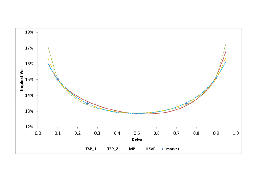
(a) TSP,MP,HSVP

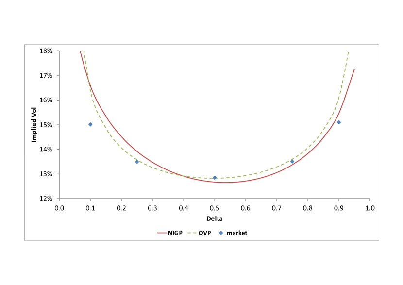
(b) NIGP,QVP

Figure 3. $\sigma\left(\Delta\right)$ calibrated to five market quotes (see Table 1) for four representative processes. The corresponding maturity is 2y.

6. Asymptotics of the Option Price in the Black-Scholes-Merton Framework

In Sections 7, 8, 9 we shall use the LL formula of Section 5 to establish a variety of asymptotic expressions for option prices and implied volatilities. Before this, however, we take a brief detour into the analysis of the limiting behavior of BS prices when variances $v$ and strikes $k$ are either large or small. This analysis is required later in order to convert option price asymptotics into implied volatility asymptotics.

As was mentioned earlier, the undiscounted price of a call option can be written in the form $\mathsf{C}^{BS}\left(v,k\right)$, where $v$ is the annualized variance, and $k$ is the log strike. The well-known relations

(6.1) $$\Phi\left(x\right)=1-\Phi\left(-x\right),\ \ \ \ \ \Phi\left(x\right)\underset{x\rightarrow-\infty}{\sim}-\frac{\phi\left(x\right)}{x}\left(1-\frac{1}{x^{2}}\right),$$

allow us to simplify the above formula in various asymptotic regimes. Specifically, we are interested in the following three cases: A) $v\rightarrow\infty$, $k=\hat{k}v$, $\hat{k}$ is fixed (long-time asymptotics); (B) $v\rightarrow 0$, $k$ is fixed (short-time asymptotics); (C) $v=\hat{v}\left|k\right|$, $\left|k\right|\rightarrow\infty$, $0\leq\hat{v}\leq 2$ (wing asymptotics). Specifically we have the following proposition:

Proposition 6.1.

In case (A) we have

(6.2) $$\mathsf{C}^{BS}\left(v,\hat{k}v\right)=\left\{\begin{array}[]{ll}\begin{array}[]{l}\left(1-e^{\hat{k}v}\right)\mathbf{1}_{\left\{\hat{k}<-\frac{1}{2}\right\}}+\mathbf{1}_{\left\{-\frac{1}{2}<\hat{k}<\frac{1}{2}\right\}}\\ +\frac{\phi\left(\left(\hat{k}-\frac{1}{2}\right)\sqrt{v}\right)}{R\left(\hat{k}\right)\sqrt{v}}\left(1-\frac{1}{v}\frac{1}{R\left(\hat{k}\right)}\left(3+\frac{1}{R\left(\hat{k}\right)}\right)\right)+...,\end{array}&\hat{k}\neq\pm\frac{1}{2},\\ \begin{array}[]{l}\frac{1}{2}\mathbf{1}_{\left\{\hat{k}=\frac{1}{2}\right\}}+\left(1-\frac{1}{2}e^{-v/2}\right)\mathbf{1}_{\left\{\hat{k}=-\frac{1}{2}\right\}}\\ -\frac{e^{\left(\hat{k}-1/2\right)v/2}}{\sqrt{v}}\left(1-\frac{1}{v}\right)+...,\end{array}&\hat{k}=\pm\frac{1}{2},\end{array}\right.$$

where

(6.3) $$R\left(\hat{k}\right)=-Q\left(i\hat{k}\right)=\hat{k}^{2}-\frac{1}{4}.$$

In case (B) we have

(6.4) $$\mathsf{C}^{BS}\left(v,k\right)=\left(1-e^{k}\right)^{+}+\phi\left(\frac{k}{\sqrt{v}}\right)\frac{e^{\frac{k}{2}}v^{3/2}}{k^{2}}\left(1-\frac{1}{8}v\right)+....$$

Finally, in case (C) we have

(6.5) $$\mathsf{C}^{BS}\left(\hat{v}\left|k\right|,k\right)=\left(1-e^{k}\right)^{+}+\frac{\phi\left(\left(1/\sqrt{\hat{v}}-\sqrt{\hat{v}}/2\right)\sqrt{\left|k\right|}\right)}{R\left(1/\hat{v}\right)\sqrt{\hat{v}\left|k\right|}}\left(1-\frac{3/\hat{v}^{2}+4}{\left(R\left(1/\hat{v}\right)\right)^{2}\hat{v}\left|k\right|}\right)+....$$

Proof.

Simple but slightly tedious application of (6.1) to BS formula (1.6), see, e.g., [117], [47], [52].    

Remark 6.1.

For case (A), it is clear that cases $\hat{k}=\pm 1/2$ require separate treatment, with $\hat{k}=1/2$ being particularly important since in order to get $\Delta\sim 1/2$, we have to have $\hat{k}-1/2\sim 1/\sqrt{v}$, in which case

$$\Delta\sim\Phi\left(\left(\hat{k}-\frac{1}{2}\right)\sqrt{v}\right)\sim\frac{1}{2}.$$

Remark 6.2.

For future reference, we wish to generalize formulas (6.2) and (6.4) and analyze the asymptotics of $\mathsf{C}^{BS}\left(\mathsf{g}\left(v\right)v,\hat{k}v\right)$, with $\mathsf{g}\left(v\right)=\left(1+\alpha_{1}/v+\alpha_{2}/v^{2}\right)$, $\hat{k}$ is fixed and $v\rightarrow\infty$, and $\mathsf{C}^{BS}\left(\mathsf{f}\left(v\right)v,k\right)$ with $\mathsf{f}\left(v\right)=\left(1+\alpha_{1}v+\alpha_{2}v^{2}\right)$, $k\neq 0$ is fixed and $v\rightarrow 0$. Straightforward computation yields

(6.6) $$\mathsf{C}^{BS}\left(\mathsf{g}\left(v\right)v,\hat{k}v\right)=\mathbf{1}_{\left\{\hat{k}<-\frac{1}{2}\right\}}\left(1-e^{\hat{k}v}\right)+\mathbf{1}_{\left\{-\frac{1}{2}<\hat{k}<\frac{1}{2}\right\}}+e^{\frac{1}{2}\alpha_{1}R\left(\hat{k}\right)}\frac{\phi\left(\left(-\hat{k}+\frac{1}{2}\right)\sqrt{v}\right)}{R\left(\hat{k}\right)\sqrt{v}}$$

$$\ \ \ \ \ \ \times\left(1-\frac{1}{v}\left(\left(\frac{1}{R\left(\hat{k}\right)}-\frac{\alpha_{1}}{2}\right)\left(3+\frac{1}{R\left(\hat{k}\right)}\right)+\frac{\alpha_{1}^{2}}{8}+\frac{R\left(\hat{k}\right)}{2}\left(\alpha_{1}^{2}-\alpha_{2}\right)\right)\right),$$

and

(6.7) $$\mathsf{C}^{BS}\left(\mathsf{f}\left(v\right)v,k\right) =\left(1-e^{k}\right)^{+}+\phi\left(\frac{k}{\sqrt{v}}\right)\frac{e^{\frac{k}{2}+\frac{\alpha_{1}k^{2}}{2}}v^{3/2}}{k^{2}}$$

$$\times\left(1-\frac{1}{8}\left(1-12\alpha_{1}+4\left(\alpha_{1}^{2}-\alpha_{2}\right)k^{2}\right)v\right)+....$$

These formulas are used below for studying the asymptotic behavior of the implied volatility in the long-time and short-time limits, respectively. A more complicated expression, which is equivalent to (6.6) is given by [47].

7. Long-time Asymptotics

7.1. General Remarks

For the purpose of establishing long-time implied volatility asymptotics via the LL formula, let us briefly introduce the so-called saddlepoint method.

Saddlepoint approximation is a method for computing integrals of the form

(7.1) $$g\left(\tau\right)=\frac{1}{2\pi}\int\limits_{\mathfrak{C}}f\left(z\right)e^{\tau S\left(z\right)}dz$$

when $\tau\rightarrow+\infty$. Here $\mathfrak{C}$ is a contour in the complex plane, and the amplitude and phase functions $f\left(z\right),S\left(z\right)$ are analytic is a domain $\mathcal{D}$ containing $\mathfrak{C}$. The extremal points of $S$, i.e. zeroes of $S^{\prime}$, are called the saddlepoints of $S$. Under reasonable conditions, the contribution to $g\left(\tau\right)$ from a vicinity of a saddlepoint $z_{0}$, where $S^{\prime\prime}\left(z_{0}\right)\neq 0$, is given by

(7.2) $$g_{z_{0},0}\left(\tau\right)=\frac{1}{\sqrt{-2\pi\tau S^{\prime\prime}\left(z_{0}\right)}}e^{\tau S\left(z_{0}\right)}f\left(z_{0}\right)\left(1+O\left(\tau^{-1}\right)\right),$$

see, e.g., [43], [80], [63], It is clear that the main contribution to the integral comes from the saddlepoints where $\mathop{\mathrm{R}e}\left[S\right]$ attains its absolute maximum. The second-order approximation has the form

(7.3) $$g_{z_{0},1}\left(\tau\right)=g_{z_{0},0}\left(\tau\right)\left(1-\frac{1}{2\tau}\left(\frac{\left(\frac{f^{\prime}\left(z_{0}\right)}{S^{\prime\prime}\left(z_{0}\right)}\right)^{\prime}}{f\left(z_{0}\right)}+\frac{5\left(S^{{}^{\prime\prime\prime}}\left(z_{0}\right)\right)^{2}}{12\left(S^{\prime\prime}\left(z_{0}\right)\right)^{3}}-\frac{S^{{}^{\prime\prime\prime\prime}}\left(z_{0}\right)}{4\left(S^{\prime\prime}\left(z_{0}\right)\right)^{2}}\right)+O\left(\tau^{-2}\right)\right).$$

Saddlepoint approximation has been successfully used by many authors for a variety of financial applications, see, e.g., [104], [71], [28], [86], among others.

7.2. BS Asymptotics via the Saddlepoint Approximation

To motivate subsequent developments, let us briefly derive some large $v$ asymptotic results for the BS case. We are specifically interested in the case when $v\rightarrow\infty$, $k=\hat{k}v$, $\hat{k}$ is fixed. We have

$$\mathsf{C}^{BS}\left(v,\hat{k}v\right)=1-\frac{1}{2\pi}\int_{-\infty}^{\infty}\frac{e^{-v\left(\frac{1}{2}Q\left(u\right)+\hat{k}\left(iu-\frac{1}{2}\right)\right)}}{Q\left(u\right)}du=1-\frac{1}{2\pi}\int_{-\infty}^{\infty}e^{vS\left(u,\hat{k}\right)}f\left(u\right)du,$$

where

$$S\left(u,\hat{k}\right)=-\frac{1}{2}Q\left(u\right)-\hat{k}\left(iu-\frac{1}{2}\right),\ \ \ \ \ f\left(u\right)=\frac{1}{Q\left(u\right)}.$$

The integrand is meromorphic in the entire complex plain where it has two simple poles located at the points

$$u_{\pm}=\pm\frac{i}{2},\ \ \ S\left(\frac{i}{2},\hat{k}\right)=\hat{k},\ \ \ S\left(-\frac{i}{2},\hat{k}\right)=0.$$

We calculate the location of the saddlepoint $u_{\ast}$ by solving the equation

$$S^{\prime}\left(u,\hat{k}\right)=-u-i\hat{k}=0,$$

so that

$$u_{\ast}=-i\hat{k},\ \ \ S^{\prime\prime}\left(u_{\ast}\right)=-1,\ \ \ S\left(u_{\ast}\right)=-\frac{1}{2}\left(\hat{k}-\frac{1}{2}\right)^{2},\ \ \ f\left(u_{\ast}\right)=-\frac{1}{R\left(\hat{k}\right)}.$$

and $R(\hat{k})$ is given by (6.3). In order to apply the saddlepoint approximation, we need to transform the contour of integration in such a way that it passes through the saddlepoint, so that its immediate vicinity dominates the entire integral. We can achieve this goal by parallel shift of the contour of integration from the real axis to the contour given by

$$\mathop{\mathrm{I}m}\left(u\right)=-\hat{k}.$$

In the process of doing so, three possibilities might occur: (A) the lower pole $u_{-}$ is crossed (OTM case); (B) no poles are crossed (near-ATM case); (C) the upper pole $u_{-}$ is crossed (ITM case). When poles are crossed, their contributions have to be computed via the Cauchy formula:

$$\Pi_{+}=e^{\hat{k}v},\ \ \ \ \ \Pi_{-}=1.$$

The contribution of the saddlepoint has the form (7.3). Summing up all these contributions, we obtain formula (6.2) of Section 6, where it is derived by elementary means.

7.3. Exponential Lévy Processes

We can now consider more general LPs.

7.3.1. Generic Exponential Lévy Processes

For a generic ELP the LL formula yields

$$C\left(\tau,k\right)=1-\frac{1}{2\pi}\int_{-\infty}^{\infty}e^{\tau S\left(u\right)}f\left(u,k\right)du,$$

where

$$S\left(u\right)=\upsilon_{0}\left(u\right)-\frac{1}{2}\sigma^{2}Q\left(u\right),\ \ \ \ \ f\left(u,k\right)=\frac{e^{-k\left(iu-\frac{1}{2}\right)}}{Q\left(u\right)},$$

where $\upsilon_{0}\left(u\right)$ is given by (5.3). Thus, for large $\tau$ the integral of interest has the form (7.1), and can be analyzed via formulas (7.2) or (7.3). However, it is more natural to assume that $k\sim\bar{k}\tau$, so that the strike moves deeper in or out of the money when maturity increases (this case is necessary to consider in order to study the asymptotic behavior of volatility as a function of delta). Under this assumption we have

$$\mathsf{C}\left(\tau,k\right)=1-\frac{1}{2\pi}\int_{-\infty}^{\infty}e^{\tau S\left(u,\bar{k}\right)}f\left(u\right)du,$$

where

$$S\left(u,\bar{k}\right)=\upsilon_{0}\left(u\right)-\frac{1}{2}\sigma^{2}Q\left(u\right)-\bar{k}\left(iu-\frac{1}{2}\right),\ \ \ \ \ f\left(u\right)=\frac{1}{Q\left(u\right)}.$$

Consider now the general case of ELPs. Since we are dealing with shifted characteristic functions, we can use symmetry and prove that the saddlepoint of interest is located on the imaginary axis. Accordingly, on the interval of analyticity of $S\left(u\right)$, given by the inequalities $\mathsf{Y}_{-}<\mathop{\mathrm{I}m}\left(u\right)<\mathsf{Y}_{+}$, we can define a real-valued function $\Xi_{01}\left(y,\bar{k}\right)$ of real arguments $y,\bar{k}$ (since on the imaginary axis the value of $S\left(u,\bar{k}\right)$ is real, see, e.g., [71], [81]) as follows

$$\Xi_{01}\left(y,\bar{k}\right)=\Xi_{0}\left(y\right)+\bar{k}\left(y+\frac{1}{2}\right),$$

where

(7.4) $$\Xi_{0}\left(y\right)=\upsilon_{0}\left(iy\right)+\frac{1}{2}\sigma^{2}R\left(y\right),$$

and $R\left(y\right)$ is given by (6.3). It is clear that we can find the location of the saddlepoint by solving the following equation

(7.5) $$\Xi_{0}^{\prime}\left(y\right)+\bar{k}=0.$$

Since, in general, this equation cannot be solved analytically, we prefer a parametric approach, by expressing $\bar{k}$ in terms of $y$, rather than the other way around. This approach leads to the following proposition.

Proposition 7.1.

Consider $y\in\left(-\mathsf{Y}_{+},\mathsf{Y}_{-}\right)$ and define $\Xi_{0}\left(y\right),\ \Xi_{1}\left(y\right)$ and $\Xi_{01,\pm}\left(y\right)$ as follows

(7.6) $$\Xi_{0}\left(y\right) =\upsilon_{0}\left(iy\right)+\frac{1}{2}\sigma^{2}R\left(y\right),\ \ \ \ \ \Xi_{1}\left(y\right)=\Xi_{0}^{\prime}\left(y\right),$$

$$\Xi_{01,\pm}\left(y\right) =\Xi_{0}\left(y\right)-\Xi_{1}\left(y\right)\left(y\pm\frac{1}{2}\right).$$

Then for $\bar{k}=-\Xi_{1}\left(y\right)$ the corresponding $\sigma_{imp}\left(\tau,\tau\bar{k}\right)$ can be written in the form

(7.7) $$\sigma_{imp}\left(\tau,\tau\bar{k}\right)=\left(a_{0}\left(y\right)+\frac{a_{1}\left(y\right)}{\tau}+\frac{a_{2}\left(y\right)}{\tau^{2}}+...\right)^{1/2},$$

so that $\sigma_{imp}\left(\tau,\tau\bar{k}\right)$ can be represented as follows

(7.8) $$\sigma_{imp}\left(\tau,\tau\bar{k}\right)=b_{0}\left(y\right)+\frac{b_{1}\left(y\right)}{\tau}+\frac{b_{2}\left(y\right)}{\tau^{2}}+....$$

where

(7.9) $$a_{0}\left(y\right) =\left(\mathrm{sign}\left(y+\frac{1}{2}\right)\sqrt{-2\Xi_{01,+}\left(y\right)}-\mathrm{sign}\left(y-\frac{1}{2}\right)\sqrt{-2\Xi_{01,-}\left(y\right)}\right)^{2},$$

(7.10) $$b_{0}\left(y\right) =a_{0}^{1/2}\left(y\right),$$

and higher order coefficients $a_{i}\left(y\right)$ and $b_{i}\left(y\right)$ have the form (D.6), (D.7).

Proof.

See Appendix D.1.    

Fundamentally, Proposition 7.1 is derived by comparing the asymptotic expansion obtained via the saddlepoint method with the asymptotic expansion for BS price given by (6.6), and balancing terms. Below we use the following notation

(7.11) $$\sigma_{imp,i}\left(y\right)=\mathop{\displaystyle\sum}\limits_{j=0}^{i}\frac{b_{j}\left(y\right)}{\tau^{j}},$$

for partial sums of an asymptotic series (7.8), and similarly in other instances.

Remark 7.1.

While in our approach Proposition 7.1 follows from asymptotic formulas for complex integrals, it can be obtained via the large deviation principle as well, see, e.g., [118], [119], [37].

7.3.2. Specific Exponential Lévy Processes

For specific ELPs, such as TSPs, NIGPs, MPs, etc., the corresponding formulas can be made explicit.

Proposition 7.2.

For TSPs, NIGPs, and MPs Proposition 7.1 holds provided that the corresponding $\Xi_{0}\left(y\right)$ are defined as follows:

(7.12) $$\Xi_{0}^{TS}\left(y\right) =\frac{1}{2}\sigma^{2}R\left(y\right)+\sum_{s=\pm}a_{s}\left(\kappa_{s}+s\left(y-\frac{1}{2}\right)\right)^{\alpha}-\gamma\left(y-\frac{1}{2}\right)+\delta,$$

$$\Xi_{0}^{NIG}\left(y\right) =\sigma^{2}\mathcal{\bar{\varkappa}}\left(\mathcal{\bar{\varkappa}}-\sqrt{\mathcal{\bar{\omega}}^{2}-y^{2}}\right),$$

$$\Xi_{0}^{M}\left(y\right) =\frac{1}{2}\sigma^{2}R\left(y\right)+\lambda\left(e^{-q\left(y-\frac{1}{2}\right)+\frac{\eta^{2}}{2}R\left(y\right)}-1-\left(1-e^{q}\right)\left(y-\frac{1}{2}\right)\right).$$

For TSPs, $y\in\left(-\kappa_{+}+\frac{1}{2},\kappa_{-}+\frac{1}{2}\right)$; for NIGPs, $y\in\left(-\bar{\omega},\bar{\omega}\right)$; for MPs, $y\in\left(-\infty,\infty\right)$.

Proof.

Proof is straightforward. For further details, see Appendices D.2, D.3, D.4, respectively.    

The quality of the saddlepoint approximation in the limit of infinite maturity for representative TSP, NIGP, and MP is illustrated in Figures 4, 5, 6, and 7, respectively. The relevant parameters are calibrated to the market. It is clear that for the calibrated TSP with $\alpha=2/3$, NIGP, and MP saddlepoint approximation is very good, while for the calibrated TSP with $\alpha=3/2$ it fails.

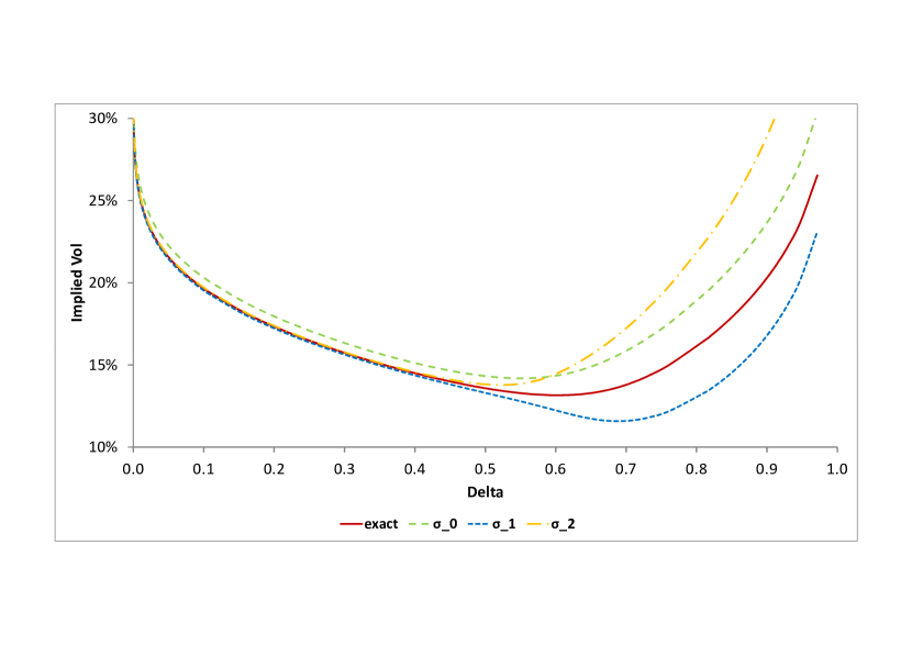
(a) T=2y

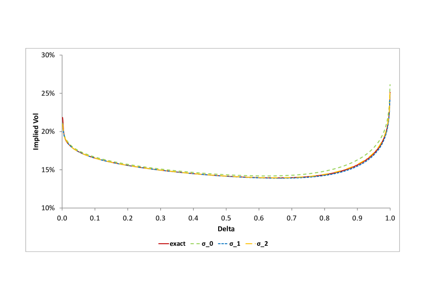
(b) T=10y

Figure 4. Comparison of the exact and asymptotic expressions for $\sigma_{imp}$ for the calibrated TSP for different maturities, $\alpha=2/3$. Here and in Figures 5, 6, and 7, ”exact” denotes the implied volatility calculated by virtue of the LL formula, while $\sigma\_0$, $\sigma\_1$, $\sigma\_2$ are given by (7.11).

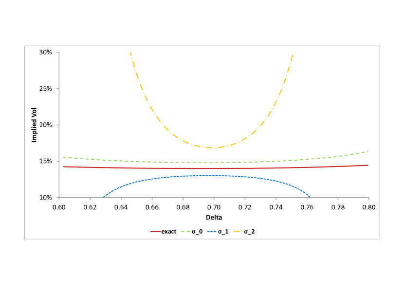
(a) T=10y

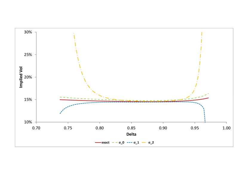
(b) T=50y

Figure 5. Comparison of the exact and asymptotic expressions for $\sigma_{imp}$ for the calibrated TSP for different maturities, $\alpha=3/2$.

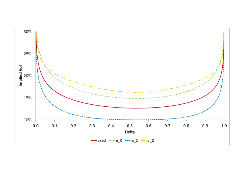
(a) T=2y

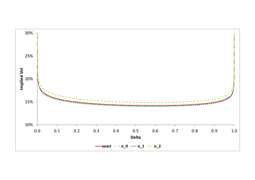
(b) T=10y

Figure 6. Comparison of the exact and asymptotic expressions for $\sigma_{imp}$ for the calibrated NIGP for different maturities.

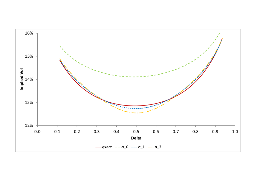
(a) T=2y

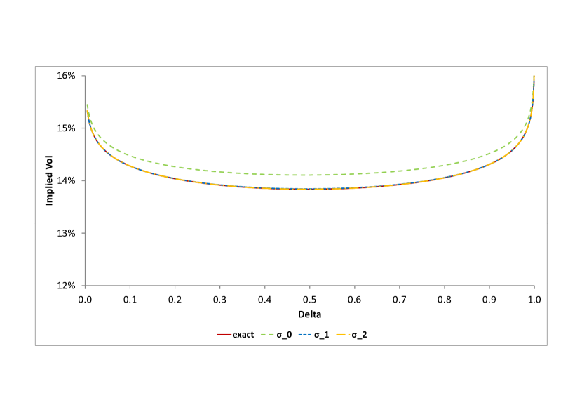
(b) T=10y

Figure 7. Comparison of the exact and asymptotic expressions for $\sigma_{imp}$ for the calibrated MP for different maturities.

Remark 7.2.

For some special cases the above formulae can be made more specific. For the general maximally skewed TSP we can solve (7.5) explicitly and avoid using the parametric representation. Specifically, we have

$$\Xi_{0}\left(y\right) =a\left(\left(\kappa-\left(y-\frac{1}{2}\right)\right)^{\alpha}-\mathsf{\zeta}\left(y-\frac{1}{2}\right)+\mathsf{\eta}\right),$$

$$\Xi_{1}\left(y\right) =a\left(-\alpha\left(\kappa-\left(y-\frac{1}{2}\right)\right)^{\alpha-1}-\mathsf{\zeta}\right)=-\bar{k},$$

where $\mathsf{\zeta}$, $\mathsf{\eta}$ are given by (4.5), so that

$$y_{\ast}\left(\bar{k}\right) =\kappa+\frac{1}{2}-\left(\frac{1}{\alpha}\left(\frac{\bar{k}}{a}-\mathsf{\zeta}\right)\right)^{\frac{1}{\alpha-1}},$$

$$\Xi_{01,\pm}\left(\bar{k}\right) =a\left(\left(1-\alpha\right)\left(\frac{1}{\alpha}\left(\frac{\bar{k}}{a}-\mathsf{\zeta}\right)\right)^{\frac{\alpha}{\alpha-1}}+\kappa\left(\frac{\bar{k}}{a}-\mathsf{\zeta}\right)+\mathsf{\eta}\right)+\frac{1}{2}\left(\bar{k}\pm\bar{k}\right),$$

$$\bar{k}_{\pm} =a\left(\alpha\left(\kappa+\frac{1}{2}\mp\frac{1}{2}\right)^{\alpha-1}+\mathsf{\zeta}\right),$$

$$\sigma_{imp,\infty}^{\left(\alpha,\kappa\right)}\left(\bar{k}\right) =\mathrm{sign}\left(\bar{k}_{-}-\bar{k}\right)\sqrt{-2\Xi_{01,+}\left(\bar{k}\right)}-\mathrm{sign}\left(\bar{k}_{+}-\bar{k}\right)\sqrt{-2\Xi_{01,-}\left(\bar{k}\right)}.$$

These formulas show that for TLGP the ATM implied volatility approaches from below the following level

$$\sigma_{imp,\infty}^{\left(1/2,\kappa\right)}\left(0\right)=2^{3/4}\vartheta^{1/4}\left(\sqrt{\kappa+1}-\sqrt{\kappa}\right)^{3/2}.$$

We compare asymptotic and exact implied volatilities for TLGP in Figures 8 (a), (b) below. These Figures show that, similarly to the general case of TSPs with $0<\alpha<1$, for TLGPs the saddlepoint approximation is acceptable.

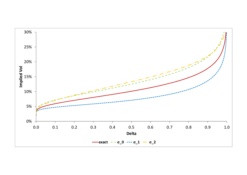
(a) T=5y

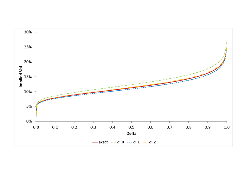
(b) T=15y

Figure 8. Comparison of the exact and asymptotic expressions for $\sigma_{imp}$ for the GLP with $\vartheta=0.0075$, $\kappa=1.0$ for different maturities. Here $\sigma_{imp,exact}$ denotes the exact volatility calculated by virtue of (4.14), while $\sigma_{imp,i}$ are given by (7.11).

Remark 7.3.

For NIGP we can easily invert the equation $\Xi_{0}^{\prime}\left(y\right)+\bar{k}=0$, and avoid using a parametric representation. We have

$$y_{0}\left(\bar{k}\right) =-\frac{\bar{\omega}\bar{k}}{\sqrt{\sigma^{4}\mathcal{\bar{\varkappa}}^{2}+\bar{k}^{2}}},\ \ \ \Xi_{01,\pm}\left(\bar{k}\right)=\sigma^{2}\mathcal{\bar{\varkappa}}^{2}-\bar{\omega}\sqrt{\sigma^{4}\mathcal{\bar{\varkappa}}^{2}+\bar{k}^{2}}\pm\frac{1}{2}\bar{k},\ \ \ \bar{k}_{\pm}=\mp\frac{\sigma^{2}}{2},$$

$$\sigma_{imp,\infty}^{NIG}\left(\bar{k}\right) =\mathrm{sign}\left(\bar{k}_{-}-\bar{k}\right)\sqrt{-2\Xi_{01,+}\left(\bar{k}\right)}-\mathrm{sign}\left(\bar{k}_{+}-\bar{k}\right)\sqrt{-2\Xi_{01,-}\left(\bar{k}\right)}.$$

Remark 7.4.

By using (4.18) which provides the call price for a NIGP explicitly, we can calculate long-time asymptotics for call prices directly, see Appendix D.3 for details. The asymptotics obtained via two complementary methods naturally agree.

7.4. Heston Stochastic Volatility Processes

Equation (5.12) shows that for the Heston model the LL exponent is not proportional to time. However, it is proportional to time to the leading order when $\tau\rightarrow\infty$. Formal expansion in powers of $\exp\left(-\tau\mathcal{Z}\left(u\right)\right)$ yields

$$\frac{E\left(\tau,u,k\right)}{Q\left(u\right)}=\frac{e^{\mathcal{A}\left(\tau,u\right)-\mathcal{B}\left(\tau,u\right)\varpi_{0}Q\left(u\right)-\tau\bar{k}\left(iu-\frac{1}{2}\right)}}{Q\left(u\right)}\sim e^{\tau S\left(u,k\right)}f\left(u\right),$$

where

(7.13) $$S\left(u,\bar{k}\right) =-\frac{\kappa\theta}{\varepsilon^{2}}\mathcal{F}_{+}\left(u\right)-\bar{k}\left(iu-\frac{1}{2}\right),$$

$$f\left(u\right) =\frac{e^{-\varpi_{0}\mathcal{F}_{+}\left(u\right)/\varepsilon^{2}}}{Q\left(u\right)\left(\frac{\mathcal{F}_{-}\left(u\right)}{2\mathcal{Z}\left(u\right)}\right)^{2\kappa\theta/\varepsilon^{2}}},$$

and $\mathcal{F}_{+}\left(u\right),\mathcal{Z}\left(u\right)$ are given by (5.13). As before, we can use saddlepoint method to obtain the asymptotic of the LL integral. It is easy to check that the corresponding saddlepoint has to be purely imaginary, so that we can proceed as before.

Proposition 7.3.

Consider $y\in\left(-\mathsf{Y}_{+},\mathsf{Y}_{-}\right)$, where

(7.14) $$\mathsf{Y}_{\pm}=\frac{\left(\mp\rho\check{\kappa}+\sqrt{\check{\kappa}^{2}+\frac{1}{4}\bar{\rho}^{2}}\right)}{\bar{\rho}^{2}},$$

and $\check{\kappa}=\hat{\kappa}/\varepsilon$, and define

(7.15) $$\Xi_{0}\left(y\right) =\frac{\kappa\theta}{\varepsilon}\left(\rho y+\check{\kappa}-\varsigma\left(y\right)\right),$$

$$\Xi_{1}\left(y\right) =\frac{\kappa\theta}{\varepsilon}\left(\rho-\frac{-\bar{\rho}^{2}y+\rho\check{\kappa}}{\varsigma\left(y\right)}\right),$$

$$\Xi_{01,\pm}\left(y\right) =\Xi_{0}\left(y\right)-\Xi_{1}\left(y\right)\left(y\pm\frac{1}{2}\right),$$

where

(7.16) $$\varsigma\left(y\right)=\sqrt{-\bar{\rho}^{2}y^{2}+2\rho\check{\kappa}y+\check{\kappa}^{2}+1/4}.$$

Then for $\bar{k}=-\Xi_{1}\left(y\right)$ the corresponding $\sigma_{imp}\left(\tau,\tau\bar{k}\right)$ can be written in the form

$$\sigma_{imp}\left(\tau,\tau\bar{k}\right)=\left(a_{0}\left(y\right)+\frac{a_{1}\left(y\right)}{\tau}+...\right)^{1/2}=b_{0}\left(y\right)+\frac{b_{1}\left(y\right)}{\tau}+...,$$

where the leading order coefficients $a_{0}\left(y\right)$ and $b_{0}\left(y\right)$ have the form (7.9), (7.10), and higher order coefficients $a_{1}\left(y\right)$ and $b_{1}\left(y\right)$ have the form (D.6), (D.7).

Proof.

The proof is similar to the one of Proposition 7.1 and is omitted for brevity.    

As expected, the leading-order term in the volatility expansion does not depend on $\varpi_{0}$. The quality of the above approximation is illustrated in Figures 9 (a), (b). These Figures show that for HSVPs the saddlepoint approximation works well.

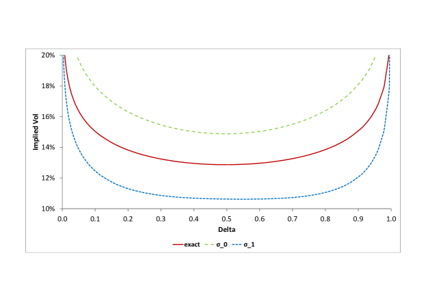
(a) T=2y

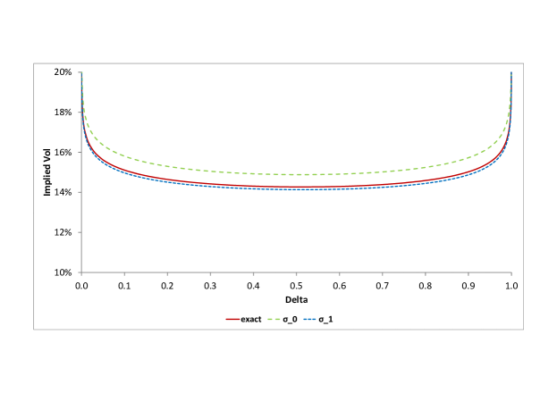
(b) T=10y

Figure 9. Comparison of the exact and asymptotic expressions for $\sigma_{imp}$ for the calibrated HSVP for different maturities. Here ”exact” denotes the implied volatility calculated by virtue of the LL formula, while $\sigma\_0$, $\sigma\_1$ (7.11).

Remark 7.5.

For HSVPs we can easily invert the equation $\Xi_{0}^{\prime}\left(y\right)+\bar{k}=0$, and avoid using the parametric representation. A simple calculation performed in Appendix D.5 yields

(7.17) $$\sigma_{imp,0}\left(\bar{k}\right) =\mathrm{sign}\left(y^{\ast}\left(\bar{k}\right)+\frac{1}{2}\right)\sqrt{-2\Xi_{01,+}\left(\bar{k}\right)}-\mathrm{sign}\left(y^{\ast}\left(\bar{k}\right)-\frac{1}{2}\right)\sqrt{-2\Xi_{01,-}\left(\bar{k}\right)},$$

$$y^{\ast}\left(\bar{k}\right) =\frac{\rho\check{\kappa}-\mathrm{sign}\left(l\right)\sqrt{\check{\kappa}^{2}-\bar{\rho}^{2}\left(\check{\kappa}^{2}-\frac{1}{4}l^{2}\right)/\left(\bar{\rho}^{2}+l^{2}\right)}}{\bar{\rho}^{2}},$$

$$\Xi_{01,\pm}\left(\bar{k}\right) =\frac{\kappa\theta}{\varepsilon l}\left(\left(\bar{\rho}^{2}+\rho l\right)y^{\ast}\left(\bar{k}\right)+\left(l-\rho\right)\check{\kappa}\right)\pm\frac{1}{2}\bar{k},$$

where $l=\rho+\varepsilon\bar{k}/\kappa\theta$.

Additional information is given in [51], [62].

8. Short-time Asymptotics

8.1. General Remarks

From the results in Proposition 5.1, and Corollary 5.2, we see that in order to analyze the asymptotic behavior of the ATM option price ($k=0$) and its derivatives for $\tau\rightarrow 0$, we need to study the following integrals

(8.1) $$\mathfrak{l}\left(\tau\right) =\frac{1}{2\pi}\int_{-\infty}^{\infty}\frac{\left(1-E\left(\tau,u\right)\right)}{Q\left(u\right)}du=\frac{1}{\pi}\mathop{\mathrm{R}e}\left\{\int_{0}^{\infty}\frac{\left(1-E\left(\tau,u\right)\right)}{Q\left(u\right)}du\right\},$$

$$\mathfrak{m}\left(\tau\right) =\frac{1}{2\pi}\int_{-\infty}^{\infty}\frac{E\left(\tau,u\right)}{Q\left(u\right)}iudu=-\frac{1}{\pi}\mathop{\mathrm{I}m}\left\{\int_{0}^{\infty}\frac{E\left(\tau,u\right)}{Q\left(u\right)}udu\right\},$$

$$\mathfrak{n}\left(\tau\right) =\frac{1}{2\pi}\int_{-\infty}^{\infty}E\left(\tau,u\right)du=\frac{1}{\pi}\mathop{\mathrm{R}e}\left\{\int_{0}^{\infty}E\left(\tau,u\right)du\right\},$$

where

$$E\left(\tau,u\right)=\exp\left(\tau\upsilon_{0}\left(u\right)-\frac{\sigma^{2}\tau}{2}Q\left(u\right)\right).$$

The relation between $\mathsf{C}\left(\tau,0\right),\mathsf{C}_{k}\left(\tau,0\right),\mathsf{C}_{kk}\left(\tau,0\right)$ and $\mathfrak{l}\left(\tau\right),\mathfrak{m}\left(\tau\right),\mathfrak{n}\left(\tau\right)$ is straightforward.

Proposition 8.1.

$\mathsf{C}\left(\tau,0\right),\mathsf{C}_{k}\left(\tau,0\right),\mathsf{C}_{kk}\left(\tau,0\right)$ can be expressed in terms of $\mathfrak{l}\left(\tau\right),\mathfrak{m}\left(\tau\right),\mathfrak{n}\left(\tau\right)$ as follows

(8.2) $$\mathsf{C}\left(\tau,0\right) =\mathfrak{l}\left(\tau\right),$$

$$\mathsf{C}_{k}\left(\tau,0\right) =\mathfrak{m}\left(\tau\right)+\frac{1}{2}\left(\mathfrak{l}\left(\tau\right)-1\right),$$

$$\mathsf{C}_{kk}\left(\tau,0\right) =\mathfrak{n}\left(\tau\right)+\mathfrak{m}\left(\tau\right)+\frac{1}{2}\left(\mathfrak{l}\left(\tau\right)-1\right).$$

Proof.

Straightforward computation.    

We assume that the implied volatility can be expanded in powers of $k$:

(8.3) $$\sigma_{imp}\left(\tau,k\right)=\sum\limits_{n\geq 0}\chi_{n}\left(\tau\right)\frac{k^{n}}{n!},$$

and demonstrate how to express $\chi_{0},\chi_{1},\chi_{2}$ in terms of $\mathfrak{l},\mathfrak{m},\mathfrak{n}$.

Proposition 8.2.

In the LL framework we get

$$\chi_{0}\left(\tau\right) \sim\mathfrak{\hat{l}}\left(\tau\right)\left(1+\frac{\mathfrak{\hat{l}}^{2}\left(\tau\right)}{24}\right)\tau^{-1/2},$$

$$\chi_{1}\left(\tau\right) \sim\mathfrak{\hat{m}}\left(\tau\right)\left(1+\frac{\mathfrak{\hat{l}}^{2}\left(\tau\right)}{8}\right)\tau^{-1/2},$$

$$\chi_{2}\left(\tau\right) \sim\left(-\frac{1}{\mathfrak{\hat{l}}\left(\tau\right)}+\frac{\mathfrak{\hat{l}}\left(\tau\right)}{24}+\frac{1}{4}\mathfrak{\hat{l}}\left(\tau\right)\mathfrak{\hat{m}}^{2}\left(\tau\right)+\mathfrak{\hat{n}}\left(\tau\right)\left(1+\frac{\mathfrak{\hat{l}}^{2}\left(\tau\right)}{8}\right)\right)\tau^{-1/2},$$

where

(8.4) $$\mathfrak{\hat{l}}\left(\tau\right)=\sqrt{2\pi}\mathfrak{l}\left(\tau\right),\ \ \ \ \ \mathfrak{\hat{m}}\left(\tau\right)=\sqrt{2\pi}\mathfrak{m}\left(\tau\right),\ \ \ \ \ \mathfrak{\hat{n}}\left(\tau\right)=\sqrt{2\pi}\mathfrak{n}\left(\tau\right).$$

Proof.

See Appendix C.    

8.2. Exponential Lévy Processes

8.2.1. Non-ATM Options on Tempered Stable Processes, Simple Heuristics

Using the LL formula, it is straightforward to develop small-time asymptotics for non-ATM options on TSPs. The argument goes as follows (see, e.g., [70] among others).

Proposition 8.3.

Assume that $\sigma=0$ and consider

$$\mathsf{C}\left(\tau,k\right)=1-\frac{1}{2\pi}\int_{-\infty}^{\infty}\frac{e^{\tau\upsilon_{0}\left(u\right)-k\left(iu-\frac{1}{2}\right)}}{Q\left(u\right)}du,\ \ \ \ \ k\neq 0,$$

where $\upsilon_{0}\left(u\right)$ is given by (5.3). If $\alpha\in\left(0,1\right)$, then

$$\frac{\partial}{\partial\tau}\mathsf{C}\left(0,k\right)\sim-\frac{1}{2\pi}\int_{-\infty}^{\infty}\frac{e^{-k\left(iu-\frac{1}{2}\right)}}{Q\left(u\right)}\upsilon_{0}\left(u\right)du,$$

where the integral clearly converges. If $\alpha\in\left(1,2\right)$, then integration by parts (which is possible because $k\neq 0$) shows that:

$$\frac{\partial}{\partial\tau}\mathsf{C}\left(\tau,k\right)\sim-\frac{1}{2\pi ik}\int_{-\infty}^{\infty}e^{-k\left(iu-\frac{1}{2}\right)}\left(\frac{\upsilon_{0}\left(u\right)}{Q\left(u\right)}\right)^{\prime}du,$$

where the integral clearly converges. Accordingly, in both cases, the time value of the call option $\mathsf{\delta C}\left(\tau,k\right)$ is linear in time,

$$\mathsf{\delta C}\left(\tau,k\right)=\mathsf{c}\left(k\right)\tau+o\left(\tau\right).$$

Proof.

See Appendix E.1.    

Broadly speaking, this result means the time decay of the time value $\mathsf{\delta C}\left(\tau,k\right)$ is much slower that in the BS case, which is of order $\exp\left(-k^{2}/2\sigma^{2}\tau\right)$, see (1.6), (6.1). To compensate for that, the corresponding non-ATM implied volatility must explode with order $O(1/\sqrt{\tau\ln(1/\tau)})$, as was already mentioned in Section 1.

8.2.2. ATM Options on Tempered Stable Processes, Simple Heuristics

For ATM options we start with a simple heuristic argument. Consider a TSP with $\sigma=0$ and $\alpha\in\left(0,1\right)$ and calculate the corresponding ATM asymptotics. From (3.10), we have

$$\mathsf{C}_{\tau}\left(\tau,x\right)=\gamma\mathsf{C}_{x}\left(\tau,x\right)+\sum\limits_{s=\pm}c_{s}\int_{0}^{\infty}\frac{\left(\mathsf{C}\left(\tau,x+sy\right)-\mathsf{C}\left(\tau,x\right)\right)e^{-\kappa_{s}y}}{y^{1+\alpha}}dy,$$

$$\mathsf{C}\left(0,x\right)=\left(e^{x}-1\right)^{+}.$$

As we already know, the martingale condition yields

$$\gamma=-\sum\limits_{s=\pm}c_{s}\int_{0}^{\infty}\frac{\left(e^{sy}-1\right)e^{-\kappa_{s}y}}{y^{1+\alpha}}dy=-p_{+}+p_{-},$$

where

$$p_{s}=sc_{s}\int_{0}^{\infty}\frac{\left(e^{sy}-1\right)e^{-\kappa_{s}y}}{y^{1+\alpha}}dy>0,\ \ \ s=\pm.$$

In order to calculate $\mathsf{C}\left(\tau,0\right)$ we discretize $x$ on a grid $x_{n}=nh$, $-N\leq x\leq N$, $\mathsf{C}_{n}\left(\tau\right)=\mathsf{C}\left(\tau,x_{n}\right)$, and use an explicit finite-difference scheme. Since we have an advection term, we have to differentiate two cases: (A) $\gamma>0$ $\left(p_{-}>p_{+}\right)$, and (B) $\gamma<0\$ $\left(p_{-}<p_{+}\right)$. In case (A) our finite-difference scheme yields

$$\frac{\mathsf{C}_{0}\left(\tau\right)}{\tau}=\gamma\frac{\left(\mathsf{C}_{1}\left(0\right)-\mathsf{C}_{0}\left(0\right)\right)}{h}+p_{+}=\gamma\frac{\left(e^{h}-1\right)}{h}+p_{+}\approx\gamma+p_{+}=p_{-}.$$

In case (B) our scheme yields

$$\frac{\mathsf{C}_{0}\left(\tau\right)}{\tau}=\gamma\frac{\left(\mathsf{C}_{0}\left(0\right)-\mathsf{C}_{-1}\left(0\right)\right)}{h}+p_{+}=p_{+}.$$

Note, in both cases differentiation is performed upstream to ensure stability of the scheme. We can combine the above formulae into one as follows

(8.5) $$\mathsf{C}\left(\tau,0\right)=\tau\max\left(p_{+},p_{-}\right).$$

We note that this formula coincides with (1.10) in Section 1. For finite variation TSPs, the ATM volatility therefore goes to zero (to ensure that $\mathsf{C}\left(\tau,0\right)$ decays linearly), in marked contrast with non-ATM volatilities, which, as was noted in Section 8.2.1, explode for $\tau\rightarrow 0$. We emphasize that the technique above does not hold for $\alpha\geq 1$, as the $p_{\pm}$ integrals diverge. We also note that the result gives us no information about the slope and convexity of the ATM implied volatility. To address these issues, we now process with a more detailed analysis.

8.2.3. Main Result for Tempered Stable Processes

In view of the LL formula, in order to be able to evaluate the short-time asymptotic behavior of $\sigma_{imp}\left(\tau,0\right)$ and its $k$-derivatives $\left.\partial_{k}\sigma_{imp}\left(\tau,k\right)\right|_{k=0}$, $\left.\partial_{k}^{2}\sigma_{imp}\left(\tau,k\right)\right|_{k=0}$, we need to evaluate the short-time limit of the three integrals in (8.1) with the shifted characteristic exponent of the form

$$\upsilon_{0}\left(u\right)=\sum_{s=\pm}a_{s}\left(\kappa_{s}-s\left(iu+\frac{1}{2}\right)\right)^{\alpha}+\gamma\left(iu+\frac{1}{2}\right)+\delta.$$

We have to distinguish four cases (A) $\alpha\in\left(0,1\right),\sigma=0$, (B) $\alpha\in\left(1,2\right),\sigma=0$, (C) $\alpha\in\left(0,1\right),\sigma>0$, (D) $\alpha\in\left(1,2\right),\sigma>0$. We calculate the corresponding integrals by scaling the independent variable $u$ as appropriate. Specifically, we use: $v=\tau u$ (case (A)); $v=\tau^{1/\alpha}u$ (case (B)); $v=\tau^{1/2}u$ (cases (C) and (D)). This technique is similar to the approach in [35], for example; in case (B), it has also been used by [116].

When considering the relevant integrals, we note that the dominated convergence theorem (DCT), which is the principal tool for studying the limiting behavior of integrals depending on parameters, cannot in all cases be applied to establish the limits for $\tau\rightarrow 0$ directly, so great case must be taken to avoid faulty conclusions. To demonstrate this, let us just consider the simple example of establishing the limit of

$$\mathfrak{\tilde{l}}\left(\tau\right)=\frac{1}{2\pi}\mathop{\displaystyle\int}\limits_{-\infty}^{\infty}\frac{1-e^{\tau\gamma\left(iu+\frac{1}{2}\right)}}{u^{2}+\frac{1}{4}}du,$$

which is similar to $\mathfrak{l}\left(\tau\right)$. Formula (5.7) shows that

$$\mathfrak{\tilde{l}}\left(\tau\right)=1-e^{\tau\gamma^{-}}\sim-\tau\gamma^{-}.$$

Now, we wish to derive this formula asymptotically. We change variables $v=\tau u$, and represent $\mathfrak{\tilde{l}}\left(\tau\right)$ in the form

$$\mathfrak{\tilde{l}}\left(\tau\right)=\tau\mathfrak{\tilde{L}}\left(\tau\right),$$

where

(8.6) $$\mathfrak{L}\left(\tau\right)=\frac{1}{2\pi}\int_{-\infty}^{\infty}\frac{1-e^{\frac{\tau\gamma}{2}+i\gamma v}}{\left(v^{2}+\frac{1}{4}\tau^{2}\right)}dv=\frac{1}{\pi}\int_{0}^{\infty}\frac{1-e^{\frac{\tau\gamma}{2}}\cos\left(\gamma v\right)}{v^{2}+\frac{1}{4}\tau^{2}}dv.$$

We notice that at $v=0$ the corresponding integrand is unbounded when $\tau\rightarrow 0$, so that we cannot apply the DCT directly. However, we can split the above integral into two parts as follows

$$\mathfrak{L}\left(\tau\right)=\mathfrak{L}_{0}^{\varepsilon}\left(\tau\right)+\mathfrak{L}_{\varepsilon}^{\infty}\left(\tau\right),$$

where

$$\mathfrak{L}_{v_{1}}^{v_{2}}\left(\tau\right)=\frac{1}{\pi}\int_{v_{1}}^{v_{2}}\frac{1-e^{\frac{\tau\gamma}{2}}\cos\left(\gamma v\right)}{v^{2}+\frac{1}{4}\tau^{2}}dv.$$

In order to evaluate $\mathfrak{L}_{0}^{\varepsilon}\left(\tau\right)$ we expand the integrand around $v=0$ and get, to the leading order in $\varepsilon$,

$$\mathfrak{L}_{0}^{\varepsilon}\left(\tau\right)\sim-\frac{\tau\gamma}{2\pi}\int_{0}^{\varepsilon}\frac{1}{v^{2}+\frac{1}{4}\tau^{2}}dv=-\frac{\gamma}{2\pi}\int_{0}^{\varepsilon/\tau}\frac{1}{Q\left(u\right)}du\sim-\frac{\gamma}{2}.$$

In order to evaluate $\mathfrak{L}_{\varepsilon}^{\infty}\left(\tau\right)$ we apply the DCT, which says that

$$\mathfrak{L}_{\varepsilon}^{\infty}\left(\tau\right)\underset{\tau\rightarrow 0}{\rightarrow}\mathfrak{L}_{\varepsilon}^{\infty}\left(0\right),$$

since the corresponding integrands are uniformly bounded, yielding:

$$\mathfrak{L}_{\varepsilon}^{\infty}\left(\tau\right)\sim\frac{1}{\pi}\int_{\varepsilon}^{\infty}\frac{1-\cos\left(\gamma v\right)}{v^{2}}dv\underset{\varepsilon\rightarrow 0}{\rightarrow}\frac{\left|\gamma\right|}{2}.$$

Thus,

$$\mathfrak{L}\left(\tau\right)\sim\frac{-\gamma+\left|\gamma\right|}{2}=-\gamma^{-},$$

which is the correct answer.

Judicious usage of the technique above, leads to the following important result:

Proposition 8.4.

Consider integrals $\mathfrak{l},\mathfrak{m},\mathfrak{n}$ defined by formulas (8.1). Their asymptotic behavior depends on $\alpha$ and $\sigma$. In cases (A)-(D) the corresponding asymptotics has the form

AC𝔏(A)τC𝔐(A)C𝔑(A)τ−1BC𝔏(B)τα′C𝔐(B)C𝔑(B)τ−α′Cσ​τ1/22​π+C𝔏(C)τC𝔐(C)τ1/212​π​σ​τ1/2+C𝔑(C)τ(1−α)/2Dσ​τ1/22​π+C𝔏(D)τ(3−α)/2C𝔐(D)τ(2−α)/212​π​σ​τ1/2+C𝔑(D)τ(1−α)/2,fragments 𝐴fragmentsC𝔏𝐴τfragmentsC𝔐𝐴fragmentsC𝔑𝐴τ1𝐵fragmentsC𝔏𝐵τsuperscript𝛼′fragmentsC𝔐𝐵fragmentsC𝔑𝐵τsuperscript𝛼′𝐶fragments𝜎superscript𝜏122𝜋C𝔏𝐶τfragmentsC𝔐𝐶τ12fragments12𝜋𝜎superscript𝜏12C𝔑𝐶τ1𝛼2𝐷fragments𝜎superscript𝜏122𝜋C𝔏𝐷τ3𝛼2fragmentsC𝔐𝐷τ2𝛼2fragments12𝜋𝜎superscript𝜏12C𝔑𝐷τ1𝛼2\begin{tabular}[]{|c|c|c|c|}\hline\cr&$\mathfrak{l}$&$\mathfrak{m}$&$\mathfrak{n}$\\ \hline\cr$A$&$C_{\mathfrak{L}}^{\left(A\right)}\tau$&$C_{\mathfrak{M}}^{\left(A\right)}$&$C_{\mathcal{\mathfrak{N}}}^{\left(A\right)}\tau^{-1}$\\ \hline\cr$B$&$C_{\mathfrak{L}}^{\left(B\right)}\tau^{\alpha^{\prime}}$&$C_{\mathfrak{M}}^{\left(B\right)}$&$C_{\mathcal{\mathfrak{N}}}^{\left(B\right)}\tau^{-\alpha^{\prime}}$\\ \hline\cr$C$&$\frac{\sigma\tau^{1/2}}{\sqrt{2\pi}}+C_{\mathfrak{L}}^{\left(C\right)}\tau$&$C_{\mathfrak{M}}^{\left(C\right)}\tau^{1/2}$&$\frac{1}{\sqrt{2\pi}\sigma\tau^{1/2}}+C_{\mathcal{\mathfrak{N}}}^{\left(C\right)}\tau^{\left(1-\alpha\right)/2}$\\ \hline\cr$D$&$\frac{\sigma\tau^{1/2}}{\sqrt{2\pi}}+C_{\mathfrak{L}}^{\left(D\right)}\tau^{\left(3-\alpha\right)/2}$&$C_{\mathfrak{M}}^{\left(D\right)}\tau^{\left(2-\alpha\right)/2}$&$\frac{1}{\sqrt{2\pi}\sigma\tau^{1/2}}+C_{\mathcal{\mathfrak{N}}}^{\left(D\right)}\tau^{\left(1-\alpha\right)/2}$\\ \hline\cr\end{tabular},

lmnlmn

where

A−((γ)−+δ+ϱ)−12sign(γ)δD(γ)B1πΓ(1−α′)rα′cos(α′χ)−1πα′χ1πΓ(1+α′)r−α′cos(α′χ)C−(12γ+δ+ϱ)−12​πγσ−1/21π2(α−1)/2Γ(α+12)pσ−(α+1)D−1π2(α−3)/2Γ(α−12)pσ−(α−1)−1π2(α−2)/2Γ(α2)qσ−α1π2(α−1)/2Γ(α+12)pσ−(α+1).fragments 𝐴fragments((γ)δϱ)fragments12sign(γ)fragmentsδ𝐷(γ)𝐵fragments1𝜋Γ(1α′)rsuperscript𝛼′(α′χ)fragments1𝜋α′χfragments1𝜋Γ(1α′)rsuperscript𝛼′(α′χ)𝐶fragments(12γδϱ)fragments12𝜋γσ12fragments1𝜋2𝛼12Γ(𝛼12)pσ𝛼1𝐷fragments1𝜋2𝛼32Γ(𝛼12)pσ𝛼1fragments1𝜋2𝛼22Γ(𝛼2)qσ𝛼fragments1𝜋2𝛼12Γ(𝛼12)pσ𝛼1\begin{tabular}[]{|c|c|c|c|}\hline\cr&$C_{\mathfrak{L}}$&$C_{\mathfrak{M}}$&$C_{\mathfrak{N}}$\\ \hline\cr$A$&$-\left(\left(\mathsf{\gamma}\right)^{-}+\mathsf{\delta}+\mathsf{\varrho}\right)$&$-\frac{1}{2}\mathrm{sign}\left(\mathsf{\gamma}\right)$&$\delta_{D}\left(\mathsf{\gamma}\right)$\\ \hline\cr$B$&$\frac{1}{\pi}\Gamma\left(1-\alpha^{\prime}\right)r^{\alpha^{\prime}}\cos\left(\alpha^{\prime}\mathsf{\chi}\right)$&$-\frac{1}{\pi}\alpha^{\prime}\mathsf{\chi}$&$\frac{1}{\pi}\Gamma\left(1+\alpha^{\prime}\right)r^{-\alpha^{\prime}}\cos\left(\alpha^{\prime}\mathsf{\chi}\right)$\\ \hline\cr$C$&$-\left(\frac{1}{2}\mathsf{\gamma}+\mathsf{\delta}+\mathsf{\varrho}\right)$&$-\frac{1}{\sqrt{2\pi}}\mathsf{\gamma}\sigma^{-1/2}$&$\frac{1}{\pi}2^{\left(\alpha-1\right)/2}\Gamma\left(\frac{\alpha+1}{2}\right)p\sigma^{-\left(\alpha+1\right)}$\\ \hline\cr$D$&$-\frac{1}{\pi}2^{\left(\alpha-3\right)/2}\Gamma\left(\frac{\alpha-1}{2}\right)p\sigma^{-\left(\alpha-1\right)}$&$-\frac{1}{\pi}2^{\left(\alpha-2\right)/2}\Gamma\left(\frac{\alpha}{2}\right)q\sigma^{-\alpha}$&$\frac{1}{\pi}2^{\left(\alpha-1\right)/2}\Gamma\left(\frac{\alpha+1}{2}\right)p\sigma^{-\left(\alpha+1\right)}$\\ \hline\cr\end{tabular}.

CLCMCNCLCMCN

Here $\alpha^{\prime}=1/\alpha$, $a_{\pm},\mathsf{\gamma,\delta,\varrho}$ are given by (4.5), $\delta_{D}\left(\mathsf{.}\right)$ is the Dirac delta function, and

$$p=\left(a_{+}+a_{-}\right)\cos\left(\frac{\pi\alpha}{2}\right)<0,\ \ q=-\left(a_{+}-a_{-}\right)\sin\left(\frac{\pi\alpha}{2}\right),\ \ r=\sqrt{p^{2}+q^{2}},\ \ \mathsf{\chi}=\arctan\left(-\frac{q}{p}\right).$$

Proof.

See Appendix E.1.    

Remark 8.1.

For $\mathfrak{m}^{\left(C\right)}$ a more accurate asymptotic expression can be derived:

$$\mathfrak{m}^{\left(C\right)}\sim\left(C_{\mathfrak{M}}^{\left(C\right)}\tau^{1/2}+D_{\mathfrak{M}}^{\left(C\right)}\tau^{\left(2-\alpha\right)/2}\right),$$

where

$$D_{\mathfrak{M}}^{\left(C\right)}=-\frac{1}{\pi}2^{\alpha/2-1}\Gamma\left(\frac{\alpha}{2}\right)q\sigma^{-\alpha}.$$

Given Proposition 8.4, we can use Proposition 8.2 to convert the price limits into the volatility limits. The results are given in Proposition 8.5 below.

Proposition 8.5.

In cases (A)-(D) we have the following expressions for $\chi_{i}$ in equation (8.3):

A2​πC𝔏(A)τ1/22​πC𝔐(A)τ−1/2N/AB2​πC𝔏(B)τα′−1/22​πC𝔐(B)τ−1/2(−12​π​C𝔏(B)+2​πC𝔑(B))τ−α′−1/2C2​πC𝔏(C)τ1/22​πC𝔐(C)2​π​C𝔏(C)σ2τ−1/2D2​πC𝔏(D)τ(2−α)/22​πC𝔐(D)τ(1−α)/22​π(C𝔏(D)σ2+C𝔑(D))τ−α/2.fragments 𝐴fragments2𝜋C𝔏𝐴τ12fragments2𝜋C𝔐𝐴τ12fragmentsNA𝐵fragments2𝜋C𝔏𝐵τsuperscript𝛼′12fragments2𝜋C𝔐𝐵τ12fragments(12𝜋superscriptsubscript𝐶𝔏𝐵2𝜋C𝔑𝐵)τsuperscript𝛼′12𝐶fragments2𝜋C𝔏𝐶τ12fragments2𝜋C𝔐𝐶fragments2𝜋superscriptsubscript𝐶𝔏𝐶superscript𝜎2τ12𝐷fragments2𝜋C𝔏𝐷τ2𝛼2fragments2𝜋C𝔐𝐷τ1𝛼2fragments2𝜋(superscriptsubscript𝐶𝔏𝐷superscript𝜎2C𝔑𝐷)τ𝛼2\begin{tabular}[]{|c|c|c|c|}\hline\cr&$\chi_{0}-\sigma$&$\chi_{1}$&$\chi_{2}$\\ \hline\cr$A$&$\sqrt{2\pi}C_{\mathfrak{L}}^{\left(A\right)}\tau^{1/2}$&$\sqrt{2\pi}C_{\mathfrak{M}}^{\left(A\right)}\tau^{-1/2}$&$N/A$\\ \hline\cr$B$&$\sqrt{2\pi}C_{\mathfrak{L}}^{\left(B\right)}\tau^{\alpha^{\prime}-1/2}$&$\sqrt{2\pi}C_{\mathfrak{M}}^{\left(B\right)}\tau^{-1/2}$&$\left(-\frac{1}{\sqrt{2\pi}C_{\mathfrak{L}}^{\left(B\right)}}+\sqrt{2\pi}C_{\mathfrak{N}}^{\left(B\right)}\right)\tau^{-\alpha^{\prime}-1/2}$\\ \hline\cr$C$&$\sqrt{2\pi}C_{\mathfrak{L}}^{\left(C\right)}\tau^{1/2}$&$\sqrt{2\pi}C_{\mathfrak{M}}^{\left(C\right)}$&$\frac{\sqrt{2\pi}C_{\mathfrak{L}}^{\left(C\right)}}{\sigma^{2}}\tau^{-1/2}$\\ \hline\cr$D$&$\sqrt{2\pi}C_{\mathfrak{L}}^{\left(D\right)}\tau^{\left(2-\alpha\right)/2}$&$\sqrt{2\pi}C_{\mathfrak{M}}^{\left(D\right)}\tau^{\left(1-\alpha\right)/2}$&$\sqrt{2\pi}\left(\frac{C_{\mathfrak{L}}^{\left(D\right)}}{\sigma^{2}}+C_{\mathfrak{N}}^{\left(D\right)}\right)\tau^{-\alpha/2}$\\ \hline\cr\end{tabular}.

(8.7) -χ0σχ1χ2-χ0σχ1χ2

Proof.

Follows from Propositions 8.2, 8.4.    

Remark 8.2.

For $\chi_{1}^{\left(C\right)},\chi_{2}^{\left(C\right)}$ more accurate asymptotic expressions can be derived:

$$\chi_{1}^{\left(C\right)} \sim\sqrt{2\pi}\left(C_{\mathfrak{M}}^{\left(C\right)}+D_{\mathfrak{M}}^{\left(C\right)}\tau^{\left(1-\alpha\right)/2}\right),$$

$$\chi_{2}^{\left(C\right)} \sim\sqrt{2\pi}\left(\frac{C_{\mathfrak{L}}^{\left(C\right)}}{\sigma^{2}}+C_{\mathfrak{N}}^{\left(C\right)}\tau^{\left(2-\alpha\right)/2}\right)\tau^{-1/2}.$$

Motivated by our discussion in Section 2, it is of interest to express these limits in terms of RRs and BFs.

Proposition 8.6.

In cases (A) - (D) we have the following expressions for RRs and BFs:

A−2​π3C𝔏(A)C𝔐(A)τ1/2N/AB−2​π3C𝔏(B)C𝔐(B)τα′−1/22​π316C𝔏(B)(−1+2πC𝔏(B)C𝔑(B)+4π(C𝔐(B))2)τα′−1/2C−πC𝔐(C)τ1/22​π316C𝔏(C)τ1/2D−πC𝔐(D)τ(2−α)/22​π316(C𝔏(D)+σ2C𝔑(D))τ(2−α)/2.fragments 𝐴fragments2superscript𝜋3C𝔏𝐴C𝔐𝐴τ12fragmentsNA𝐵fragments2superscript𝜋3C𝔏𝐵C𝔐𝐵τsuperscript𝛼′12fragments2superscript𝜋316C𝔏𝐵(12πC𝔏𝐵C𝔑𝐵4π(C𝔐𝐵)2)τsuperscript𝛼′12𝐶fragmentsπC𝔐𝐶τ12fragments2superscript𝜋316C𝔏𝐶τ12𝐷fragmentsπC𝔐𝐷τ2𝛼2fragments2superscript𝜋316(C𝔏𝐷σ2C𝔑𝐷)τ2𝛼2\begin{tabular}[]{|c|c|c|}\hline\cr&$RR$&$BF$\\ \hline\cr$A$&$-\sqrt{2\pi^{3}}C_{\mathfrak{L}}^{\left(A\right)}C_{\mathfrak{M}}^{\left(A\right)}\tau^{1/2}$&$N/A$\\ \hline\cr$B$&$-\sqrt{2\pi^{3}}C_{\mathfrak{L}}^{\left(B\right)}C_{\mathfrak{M}}^{\left(B\right)}\tau^{\alpha^{\prime}-1/2}$&$\frac{\sqrt{2\pi^{3}}}{16}C_{\mathfrak{L}}^{\left(B\right)}\left(-1+2\pi C_{\mathfrak{L}}^{\left(B\right)}C_{\mathfrak{N}}^{\left(B\right)}+4\pi\left(C_{\mathfrak{M}}^{\left(B\right)}\right)^{2}\right)\tau^{\alpha^{\prime}-1/2}$\\ \hline\cr$C$&$-\pi C_{\mathfrak{M}}^{\left(C\right)}\tau^{1/2}$&$\frac{\sqrt{2\pi^{3}}}{16}C_{\mathfrak{L}}^{\left(C\right)}\tau^{1/2}$\\ \hline\cr$D$&$-\pi C_{\mathfrak{M}}^{\left(D\right)}\tau^{\left(2-\alpha\right)/2}$&$\frac{\sqrt{2\pi^{3}}}{16}\left(C_{\mathfrak{L}}^{\left(D\right)}+\sigma^{2}C_{\mathfrak{N}}^{\left(D\right)}\right)\tau^{\left(2-\alpha\right)/2}$\\ \hline\cr\end{tabular}.

RRBFRRBF

Proof.

Combining equations (2.2) and (2.3) we easily get

(8.8) $$RR\left(\tau\right)\sim-\sqrt{\frac{\pi}{2}}\chi_{0}\chi_{1}\tau^{1/2},$$

(8.9) $$BF\left(\tau\right)\sim\frac{\pi}{32}\chi_{0}\left(2\chi_{0}\chi_{2}-\chi_{0}\chi_{1}+4\chi_{1}^{2}\right)\tau,$$

The Proposition now follows directly from Proposition 8.5.    

Remark 8.3.

For $RR^{\left(C\right)}$, $RR^{\left(D\right)}$, $BF^{\left(B\right)}$, $BF^{\left(C\right)}$ more accurate asymptotic expressions can be derived:

$$RR^{\left(C\right)} \sim-\sqrt{2\pi^{3}}\left(\frac{1}{\sqrt{2\pi}}+C_{\mathfrak{L}}^{\left(C\right)}\tau^{1/2}\right)C_{\mathfrak{M}}^{\left(C\right)}\tau^{1/2},$$

$$RR^{\left(D\right)} \sim-\sqrt{2\pi^{3}}\left(\frac{1}{\sqrt{2\pi}}+C_{\mathfrak{L}}^{\left(D\right)}\tau^{\left(2-\alpha\right)/2}\right)C_{\mathfrak{M}}^{\left(D\right)}\tau^{\left(2-\alpha\right)/2},$$

$$BF^{\left(B\right)} \sim\frac{\sqrt{2\pi^{3}}}{16}C_{\mathfrak{L}}^{\left(B\right)}\left(-1+2\pi C_{\mathfrak{L}}^{\left(B\right)}C_{\mathfrak{N}}^{\left(B\right)}+4\pi\left(C_{\mathfrak{M}}^{\left(B\right)}\right)^{2}-\pi C_{\mathfrak{L}}^{\left(B\right)}C_{\mathfrak{M}}^{\left(B\right)}\tau^{\alpha^{\prime}}\right)\tau^{\alpha^{\prime}-1/2},$$

$$BF^{\left(C\right)} \sim\frac{\sqrt{2\pi^{3}}}{16}\left(C_{\mathfrak{L}}^{\left(C\right)}+\sigma^{2}C_{\mathfrak{N}}^{\left(C\right)}\tau^{\left(1-\alpha\right)/2}\right)\tau^{1/2}.$$

Examination of the table in Proposition 8.6 shows that in all cases (with the exception of the degenerate case (A)), RRs and BFs go to zero for small $\tau$. In other words, TSPs cannot produce finite limits for RRs and BFs for $\tau\rightarrow 0$. On the other hand, the rate of decay is generally slower than for regular diffusions.

8.2.4. Tests

In order to study the quality of the above asymptotic formulas in detail we start with a representative LGP considered in Proposition 4.3. As in Section 7.3.2, we choose for illustrative purposes $\vartheta=0.0075$, $\kappa_{-}=1.00$. Straightforward calculation yields $C_{\mathfrak{L}}^{\left(A\right)}=0.0507$, $C_{\mathfrak{M}}^{\left(A\right)}=-0.5$, $C_{\mathfrak{N}}^{\left(A\right)}=0.0$. The quality of the corresponding asymptotic formulas vs. exact analytical expressions calculated in Proposition 4.3 is shown in Table 4. Here and below $\bar{C}$ and $C$ stand for the values calculated numerically and analytically, respectively, and similarly for other quantities of interest.

$\log_{10}\left(\tau\right)$ -2 -4 -6 $\bar{C}_{\mathfrak{L}}^{(A)}/C_{\mathfrak{L}}^{(A)}$ 0.941 0.994 0.999 $\bar{C}_{\mathfrak{M}}^{(A)}/C_{\mathfrak{M}}^{(A)}$ 0.941 0.994 0.999 $\bar{C}_{\mathfrak{N}}^{(A)}$ 0.304 0.030 0.003

Table 4. Analytical vs. numerical values for $C_{\mathfrak{L}}^{\left(A\right)}$, $C_{\mathfrak{M}}^{\left(A\right)}$, $C_{\mathfrak{N}}^{\left(A\right)}$.

Next, we up the ante and consider realistic TSPs. Table 5 lists their parameters as well as the values of $C_{\mathfrak{L}}$, $C_{\mathfrak{M}}$, $C_{\mathfrak{N}}$ as computed by Proposition 8.4. The quality of the corresponding asymptotic formulas is summarized in Tables 6, 7.

$\alpha$ $c_{+}$ $c_{-}$ $\kappa_{+}$ $\kappa_{-}$ $\sigma$ $C_{\mathfrak{L}}$ $C_{\mathfrak{M}}$ $C_{\mathfrak{N}}$ A 0.66 0.1305 0.0615 6.5022 3.0888 0.00 0.1863 0.5000 0.0000 B 1.50 0.0069 0.0063 1.9320 0.4087 0.00 0.0670 0.0096 3.6492 C 0.66 0.0521 0.0245 6.5022 3.0888 0.10 0.0599 0.1353 -2.2867 D 1.50 0.0028 0.0025 1.9320 0.4087 0.10 0.0192 0.0052 -0.9610

Table 5. Parameters for four representative TSPs and analytical values for $C_{\mathfrak{L}}$, $C_{\mathfrak{M}}$, $C_{\mathfrak{N}}$. Parameters for processes (A) and (B) are approximately calibrated to the market vols for 2y options; parameters for processes (C) and (D) are chosen in such a way that the market ATM vol for 2y options is recovered. In addition, $D_{\mathfrak{M}}^{\left(C\right)}=-0.2395$.

$\log\left(\tau\right)$ -2 -4 -6 -8 -10 A $\bar{C}_{\mathfrak{L}}^{(A)}/C_{\mathfrak{L}}^{(A)}$ 0.74 0.94 0.99 1.00 1.00 A $\bar{C}_{\mathfrak{M}}^{(A)}/C_{\mathfrak{M}}^{(A)}$ 0.60 0.92 0.81 0.76 1.28 B $\bar{C}_{\mathfrak{L}}^{(B)}/C_{\mathfrak{L}}^{(B)}$ 0.92 0.98 1.00 1.00 1.00 B $\bar{C}_{\mathfrak{M}}^{(B)}/C_{\mathfrak{M}}^{(B)}$ 0.43 0.86 0.97 0.99 1.00 B $\bar{C}_{\mathfrak{N}}^{(B)}/C_{\mathfrak{N}}^{(B)}$ 1.00 1.00 1.00 1.00 1.00 C $\bar{C}_{\mathfrak{L}}^{(C)}/C_{\mathfrak{L}}^{(C)}$ 0.51 0.76 0.87 0.95 0.98 C $\bar{C}_{\mathfrak{M}}^{(C)}/C_{\mathfrak{M}}^{(C)}$ 0.29 0.63 0.82 0.92 0.96 C $\bar{D}_{\mathfrak{M}}^{(C)}/D_{\mathfrak{M}}^{(C)}$ 0.86 0.96 0.99 1.00 1.00 C $\bar{C}_{\mathfrak{N}}^{(C)}/C_{\mathfrak{N}}^{(C)}$ 0.75 0.94 0.99 1.00 1.00 D $\bar{C}_{\mathfrak{L}}^{(D)}/C_{\mathfrak{L}}^{(D)}$ 0.83 0.94 0.98 0.99 1.00 D $\bar{C}_{\mathfrak{M}}^{(D)}/C_{\mathfrak{M}}^{(D)}$ 0.27 0.72 0.91 0.97 0.99 D $\bar{C}_{\mathfrak{N}}^{(D)}/C_{\mathfrak{N}}^{(D)}$ 0.91 0.97 0.99 1.00 1.00

Table 6. Analytical vs. numerical values for $C_{\mathfrak{L}}$, $C_{\mathfrak{M}}$, $C_{\mathfrak{N}}$, and $D_{\mathfrak{M}}^{\left(C\right)}$.

To numerically examine the performance of the short-time asymptotic expansions, Table 7 compares the asymptotic results given by (8.7) with the results for $\chi_{0}-\sigma$, $\chi_{1}$, and $\chi_{2}$ obtained by a direct computation of the LL integrals in Equations (5.1), (5.4), (5.5). Note that high-precision numerical computation of these integrals is a rather delicate affair; to ensure stable results, we used adaptive Gauss-Kronrod quadrature combined with both a judicious choice of integration region and a very high number of integration nodes (often exceeding $10^{5}$ nodes). Table 7 provides proof for the validity of the results given by (8.7), as the exact and asymptotic results converge to each other for sufficiently small $\tau$. Unfortunately, this convergence is rather slow and only truly satisfactory for $\tau$ around $10^{-4}$ years, i.e. for time-scales in the order of minutes or seconds. While the asymptotic expressions do provide the correct limiting behavior, it is therefore questionable how useful they are for practical work.

$\log\left(\tau\right)$ 0 -2 -4 -6 -8 -10 A $\log\left(\chi_{0}-\sigma\right)$ -0.92 -1.46 -2.36 -3.34 -4.33 -5.33 A $\log\left(\bar{\chi}_{0}-\sigma\right)$ -0.33 -1.33 -2.33 -3.33 -4.33 -5.33 A $\log\left(\chi_{1}\right)$ -1.34 0.88 2.06 3.01 3.98 5.20 A $\log\left(\bar{\chi}_{1}\right)$ 0.10 1.10 2.10 3.10 4.10 5.10 B $\log\left(\chi_{0}-\sigma\right)$ -0.91 -1.14 -1.45 -1.78 -2.11 -2.44 B $\log\left(\bar{\chi}_{0}-\sigma\right)$ -0.77 -1.11 -1.44 -1.77 -2.11 -2.44 B $\log\left(\chi_{1}\right)$ -1.87 + $\pi i$ -0.98 0.32 1.37 2.38 3.38 B $\log\left(\bar{\chi}_{1}\right)$ -1.62 -0.62 0.38 1.38 2.38 3.38 B $\log\left(\chi_{2}\right)$ 0.23 2.78 5.16 7.50 9.84 12.17 B $\log\left(\bar{\chi}_{2}\right)$ 0.51 2.84 5.17 7.51 9.84 12.17 C $\log\left(\chi_{0}-\sigma\right)$ -1.57 - 2.11 -2.94 -3.88 -4.85 –5.83 C $\log\left(\bar{\chi}_{0}-\sigma\right)$ -0.82 -1.82 -2.82 -3.82 -4.82 -5.82 C $\log\left(\chi_{1}\right)$ -2.75 -1.00 -0.67 -0.55 -0.51 -0.49 C $\log\left(\bar{\chi}_{1}\right)$ -0.47 -0.47 -0.47 -0.47 -0.47 -0.47 C $\log\left(\chi_{2}\right)$ -0.25 1.71 3.00 4.10 5.14 6.16 C $\log\left(\bar{\chi}_{2}\right)$ 1.18 2.18 3.18 4.18 5.18 6.18 D $\log\left(\chi_{0}-\sigma\right)$ -1.56 -1.90 -2.34 -2.83 -3.32 -3.82 D $\log\left(\bar{\chi}_{0}-\sigma\right)$ -1.32 -1.82 -2.32 -2.82 -3.32 -3.82 D $\log\left(\chi_{1}\right)$ -2.42 + $\pi i$ -1.95 -1.03 -0.43 0.10 0.61 D $\log\left(\bar{\chi}_{1}\right)$ -1.88 -1.38 -0.88 -0.38 0.12 0.62 D $\log\left(\chi_{2}\right)$ -0.36 1.63 3.30 4.86 6.37 7.88 D $\log\left(\bar{\chi}_{2}\right)$ 0.38 1.88 3.38 4.88 6.38 7.88

Table 7. Analytical and numerical values for $\log(\chi_{0}-\sigma)$, $\log\left(\chi_{1}\right)$, and $\log\left(\chi_{2}\right)$ as functions of $\log\left(1/\tau\right)$.

To further illustrate the convergence of exact and asymptotic results, Figure 10 contains log-log plots of the short-time behavior of $\chi_{0}-\sigma$, $\chi_{1}$, and $\chi_{2}$, for test case C ($1<\alpha<2$, $\sigma>0$). It is evident that the straight-line behavior predicted by (8.7) is not realized for values of $\tau$ larger than, at most, a few hours.

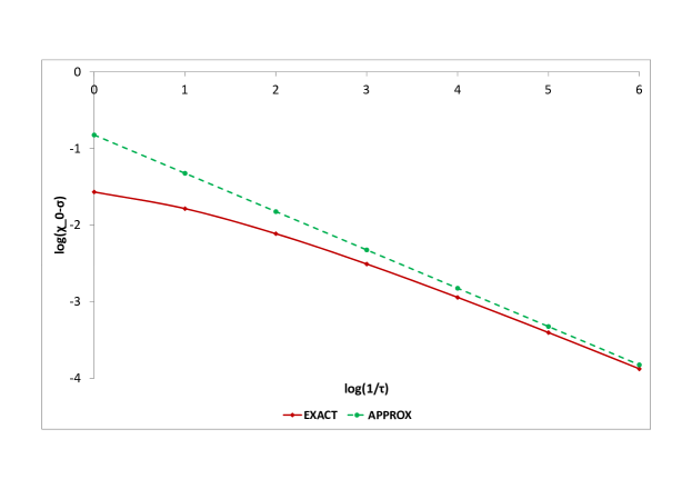
(a) $\chi_{0}-\sigma$

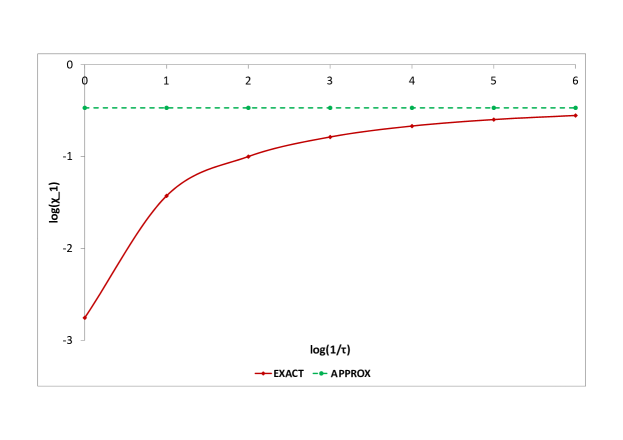
(b) $\chi_{1}$

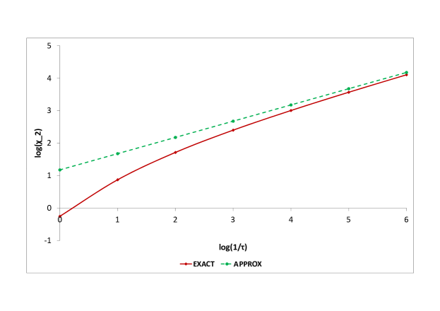
(c) $\chi_{2}$

Figure 10. Comparison of the exact and asymptotic short-time behavior of $\chi_{0}\left(\tau\right)-\sigma$, $\chi_{1}\left(\tau\right)$, and $\chi_{2}\left(\tau\right)$, for test case C.

8.2.5. Options on Normal Inverse Gaussian Processes

By using (4.16), we can calculate short-time asymptotics for call prices both directly and via the LL formula.

Proposition 8.7.

When $k\neq 0$ the asymptotic behavior of the time value of the call option $\mathsf{\delta C}^{NIG}\left(v,k\right)$ and its derivatives is linear in time

$$\frac{\partial^{p}\mathsf{\delta C}^{NIG}\left(v,k\right)}{\partial k^{p}}=\mathsf{c}_{p}^{NIG}\left(k\right)v+o\left(v\right),\ \ \ \ \ k\neq 0,$$

where $v=\sigma^{2}\tau$.

Proof.

See Appendix E.2.    

When $k=0$, we need to analyze the asymptotic behavior of of the integrals $\mathfrak{l},\mathfrak{m},\mathfrak{n}$ given by (8.1) with $E^{NIG}\left(v,u\right)$ of the form

(8.10) $$E^{NIG}\left(v,u\right)=\exp\left(v\mathcal{\bar{\varkappa}}\left(\mathcal{\bar{\varkappa}}-\sqrt{\mathcal{\bar{\omega}}^{2}+u^{2}}\right)\right).$$

Proposition 8.8.

Consider $\mathfrak{l},\mathfrak{m},\mathfrak{n}$ defined by formulas (8.1) with $E^{NIG}\left(v,u\right)$ given by (8.10) and the ATM call price $\mathsf{C}^{NIG}\left(v,0\right)$ and its derivatives with respect to log-strike $k$. Their asymptotic behavior is given by

$$\mathfrak{l}\left(v\right) \sim\mathsf{C}^{NIG}\left(v,0\right)\sim-\frac{\mathcal{\bar{\varkappa}}v\ln\left(v\right)}{\pi},$$

$$\mathfrak{m}\left(v\right) \sim\mathsf{C}_{k}^{NIG}\left(v,0\right)\sim-\frac{1}{2},$$

$$\mathfrak{n}\left(v\right) \sim\mathsf{C}_{kk}^{NIG}\left(v,0\right)\sim\frac{1}{\pi\mathcal{\bar{\varkappa}}v}.$$

Proof.

See Appendix E.2.    

As for TSPs, the rate of convergence of the corresponding integrals for NIGPs is slow.

8.2.6. Options on Merton Processes

As was mentioned earlier, MPs do not belong to the TS class. Nevertheless, they can be analyzed by the same methods. For brevity we assume that $\sigma=0$. As before, we need to evaluate the integrals $\mathfrak{l},\mathfrak{m},\mathfrak{n}$ given by (8.1) with $E^{M}\left(v,u\right)$ of the form

(8.11) $$E^{M}\left(v,u\right)=\exp\left(v\left(\left(e^{q\left(iu+1/2\right)-\eta^{2}Q\left(u\right)/2}-1\right)+\left(1-e^{q}\right)\left(iu+\frac{1}{2}\right)\right)\right).$$

Proposition 8.9.

Consider $\mathfrak{l},\mathfrak{m},\mathfrak{n}$ defined by formulas (8.1) with $E^{M}\left(\tau,u\right)$ given by (8.11) and the ATM call price $\mathsf{C}^{M}\left(v,0\right)$ and its derivatives with respect to log-strike $k$. Their asymptotic behavior is given by

$$\mathfrak{l}\left(v\right) \sim\mathsf{C}^{M}\left(v,0\right)\sim v\left(\left(1-e^{q}\right)^{+}+e^{q}\mathsf{C}^{BS}\left(\eta,-q\right)\right),$$

$$\mathfrak{m}\left(v\right) \sim\mathsf{C}_{k}^{M}\left(v,0\right)\sim-\frac{1}{2}\mathrm{sign}\left(1-e^{q}\right),$$

$$\mathfrak{n}\left(v\right) \sim\mathsf{C}_{kk}^{M}\left(v,0\right)\sim\frac{1}{v}\delta\left(1-e^{q}\right).$$

where $v=\lambda\tau$.

Proof.

See Appendix E.3.    

We can obtain the result of Proposition 8.9 directly from the Merton’s formula. To see this, let $\mathsf{C}\left(\tau,\bar{k}\tau;\sigma\right)$ be the normalized BS price of a call option considered as a function of time, time-proportional log-strike, and volatility,

$$\mathsf{C}\left(\tau,\bar{k}\tau;\sigma\right)=\Phi\left(\left(-\frac{\bar{k}}{\sigma}+\frac{\sigma}{2}\right)\sqrt{\tau}\right)-e^{\bar{k}\tau}\Phi\left(-\left(\frac{\bar{k}}{\sigma}+\frac{\sigma}{2}\right)\sqrt{\tau}\right).$$

To the leading order we can represent the normalized price of an ATM call option on a MP as follows

$$\mathsf{C}^{M}\left(\tau,0\right)\sim\mathsf{C}\left(\tau,-\lambda\tau\left(1-e^{q}\right);0\right)+\lambda\tau e^{q}\mathsf{C}\left(\tau,-\left(\lambda\tau\left(1-e^{q}\right)+q\right);\frac{\eta}{\sqrt{\tau}}\right).$$

We have

$$\mathsf{C}\left(\tau,-\lambda\tau\left(1-e^{q}\right);0\right) =\left(1-e^{-\lambda\tau\left(1-e^{q}\right)}\right)^{+}=\lambda\tau\left(1-e^{q}\right)^{+},$$

$$\lambda\tau e^{q}\mathsf{C}\left(\tau,-\left(\lambda\tau\left(1-e^{q}\right)+q\right);\frac{\eta}{\sqrt{\tau}}\right) \sim\lambda\tau e^{q}\left(\Phi\left(\frac{q}{\eta}+\frac{\eta}{2}\right)-e^{-q}\Phi\left(\frac{q}{\eta}-\frac{\eta}{2}\right)\right).$$

Accordingly,

$$\mathsf{C}^{M}\left(\tau,0\right)\sim\lambda\tau\left(\left(1-e^{q}\right)^{+}+e^{q}\mathsf{C}^{BS}\left(\eta,-q\right)\right).$$

in agreement with our previous result (recall that, from (8.2) $\mathsf{C}=\mathfrak{l}$). Expressions for $\mathfrak{m}$ and $\mathfrak{n}$ can be obtained in the same manner.

8.3. Local Volatility Processes

Consider the general local volatility case and assume that an underlying is governed by the SDE of the form

(8.12) $$dF\left(t\right)=\sigma_{loc}^{N}\left(F\left(t\right)\right)dW\left(t\right),\ \ \ \ \ F\left(0\right)=F_{0},$$

where $\sigma_{loc}^{N}\left(F\right)$ is the so-called Normal local volatility. The corresponding log-normal local volatility is given by $\sigma_{loc}^{N}\left(F\right)/F$, for brevity we denote it as $\sigma_{loc}\left(F\right)$. We consider options on the underlying driven by Brownian motion with local volatility described by (8.12). When $F_{t}$ is driven by a Brownian process with local volatility, we call the corresponding process a local volatility process (LVP). It is well-known (and had been established via asymptotic methods by [53] a long time ago) that the corresponding short term implied volatility $\sigma_{imp}\left(\tau,k\right)$, is independent of $\tau$ to the leading order while RRs and BFs are proportional to $\tau^{1/2}$and $\tau$, respectively. Thus, market observed behavior of FX volatilities (see Table 1) cannot be explained in the local volatility framework. Let us assume that

$$\sigma_{loc}\left(k\right)=\sum\limits_{n\geq 0}\xi_{n}\frac{k^{n}}{n!},\ \ \ \ \ \sigma_{imp}\left(\tau,k\right)=\sum\limits_{n\geq 0}\chi_{n}\frac{k^{n}}{n!},$$

and express $\chi_{n}$, RRs and BFs in terms of $\xi_{n}$ and $\tau$.

Proposition 8.10.

In the limit of $\tau\rightarrow 0$ the implied volatility $\sigma_{imp,0}\left(k\right)$ can be written as

(8.13) $$\sigma_{imp,0}\left(k\right)=\left\{\begin{array}[]{cc}\frac{k}{\int_{0}^{k}\frac{dk^{\prime}}{\sigma_{loc}\left(k^{\prime}\right)}}=\frac{k}{\int_{F_{0}}^{K}\frac{dK^{\prime}}{\sigma_{loc}^{N}\left(K^{\prime}\right)}},&k\neq 0,\\ \sigma_{loc}\left(0\right),&k=0,\end{array}\right.\equiv b_{0}\left(k\right).$$

Accordingly, the coefficients $\chi_{n}^{\left(0\right)}$ can be expressed in terms of $\xi_{n}$ as follows:

(8.14) $$\chi_{0}^{\left(0\right)}=\xi_{0},\ \ \ \ \ \chi_{1}^{\left(0\right)}=\frac{\xi_{1}}{2},\ \ \ \ \ \chi_{2}^{\left(0\right)}=\frac{2\xi_{0}\xi_{2}-\xi_{1}^{2}}{6\xi_{0}},$$

while RRs and BFs we have the following expressions:

(8.15) $$RR\left(\tau\right)\sim-\sqrt{\frac{\pi}{8}}\xi_{0}\xi_{1}\tau^{1/2},$$

(8.16) $$BF\left(\tau\right)\sim\frac{\pi}{32}\xi_{0}\left(-\frac{1}{2}\xi_{0}\xi_{1}+\frac{4}{3}\xi_{0}\xi_{2}+\frac{1}{3}\xi_{1}^{2}\right)\tau.$$

Proof.

Formula (8.13) is given in [5], [19], [20], [40]. Rewriting it in the form

(8.17) $$\frac{k}{\sigma_{imp}\left(k\right)}=\int_{0}^{k}\frac{d\xi}{\sigma_{loc}\left(\xi\right)}.$$

and differentiating (8.17) with respect to $k$ three times, we obtain (8.14). Substituting (8.14) in (8.8), (8.9), we obtain (8.15), (8.16).    

Remark 8.4.

More accurate formulas incorporating linear dependence on $\tau$ are also well-known (see,e.g., [5], [57], [75], [58]):

(8.18) $$\sigma_{imp,1}\left(\tau,k\right)=b_{0}\left(k\right)+\tau b_{1}\left(k\right),$$

where

$$b_{1}\left(k\right)=\left\{\begin{array}[]{ll}\frac{b_{0}^{3}\left(k\right)}{2k^{2}}\ln\left(\frac{\sigma_{loc}\left(0\right)\sigma_{loc}\left(k\right)}{b_{0}^{2}\left(k\right)}\right),&k\neq 0,\\ \frac{\sigma_{loc}^{2}\left(0\right)b_{0,kk}\left(0\right)}{4},&k=0.\end{array}\right.$$

QVPs can be used as a convenient test bed for checking the asymptotic formulas (8.13) and (8.18). For the quadratic volatility model with negative real roots, say, the terms in (8.18) become especially simple:

$$b_{0}\left(k\right)=\frac{\mathfrak{aq}k}{\mathfrak{S}\left(k\right)},$$

$$b_{1}\left(k\right)=\left\{\begin{array}[]{cc}\frac{\mathfrak{a}^{3}\mathfrak{q}^{3}k}{2\mathfrak{S}^{3}\left(k\right)}\ln\left(\frac{\left(\left(1-\mathfrak{p}\right)^{2}+\mathfrak{q}^{2}\right)\left(\left(e^{k}-\mathfrak{p}\right)^{2}+\mathfrak{q}^{2}\right)\mathfrak{S}^{2}\left(k\right)}{e^{k}\mathfrak{q}^{2}k^{2}}\right),&k\neq 0\\ \frac{1}{24}\mathfrak{a}^{3}\left(\left(1-\mathfrak{p}\right)^{2}+\mathfrak{q}^{2}\right)\left(\left(\left(1-\mathfrak{p}\right)^{2}+\mathfrak{q}^{2}\right)^{2}+4\mathfrak{q}^{2}\right),&k=0.\end{array}\right.$$

where

$$\mathfrak{S}\left(k\right)=\arctan\left(\frac{\mathfrak{p}-1}{\mathfrak{q}}\right)-\arctan\left(\frac{\mathfrak{p}-e^{k}}{\mathfrak{q}}\right).$$

The quality of these approximations versus the exact expression obtained Proposition 5.4 is very good, as is shown in Figure 11. However, it is clear that having substantial risk-reversal and straddles for short maturities is not feasible in this setting when parameters are of order unity.

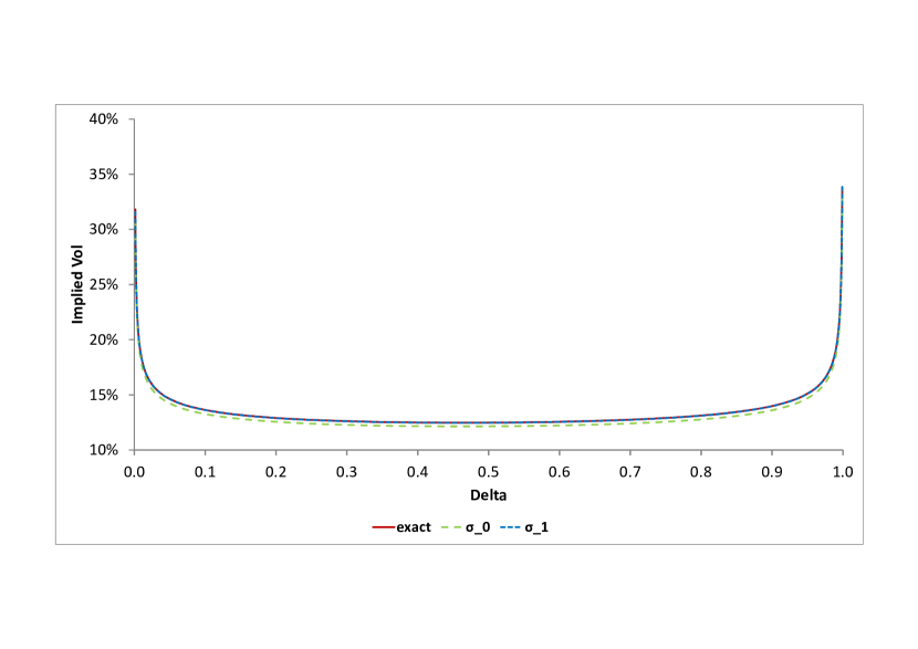
(a) T=1y

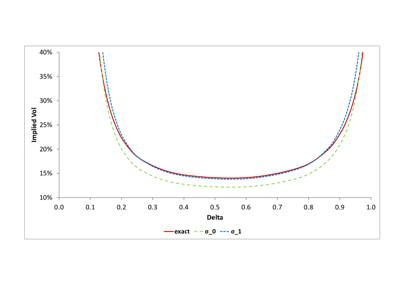
(b) T=5y

Figure 11. Comparison of the exact and asymptotic expressions for $\sigma_{imp}$ for the calibrated QVP for different maturities. Here ”exact” denotes the exact volatility calculated by virtue of the formula (5.10), while $\sigma\_0$, $\sigma\_1$ are given by (8.13), (8.18).

8.4. Heston Stochastic Volatility Processes

We can easily analyze the asymptotic behavior of the implied volatility for the Heston model either by using the LL formula or by direct computation, see e.g., [71], [73], [74], [75], [77], [91], [49], [121], [50]. Comparison of the asymptotic and exact formulas can be performed by computing the relevant integrals numerically, which, by now is a well-understood procedure, see, e.g., [61], [110]. In view of Proposition 8.2, in order to describe the asymptotic behavior of the implied volatility in the Heston framework, we need to evaluate asymptotically the corresponding integrals $\mathfrak{l},\mathfrak{m},\mathfrak{n}$.

Proposition 8.11.

The asymptotic behavior of the integrals $\mathfrak{\hat{l}},\mathfrak{\hat{m}},\mathfrak{\hat{n}}$ defined by (8.4)is described as follows

(8.19) $$\mathfrak{\hat{l}}\left(\tau\right) \sim\sqrt{\varpi_{0}\tau}\left(1+\lambda_{1}\tau+\lambda_{2}\tau^{2}+...\right),$$

$$\mathfrak{\hat{m}}\left(\tau\right) \sim\sqrt{\varpi_{0}\tau}\frac{\rho\varepsilon}{4\varpi_{0}}\left(1+\mu_{1}\tau+...\right),$$

$$\mathfrak{\hat{n}}\left(\tau\right) \sim\frac{1}{\sqrt{\varpi_{0}\tau}}\left(1+\nu_{1}\tau+\nu_{2}\tau^{2}+...\right),$$

where the corresponding $\lambda_{i},\mu_{i},\nu_{i}$ are given by (E.1).

Proof.

See Appendix E.4.    

Proposition 8.12.

For HSVPs, we have the following expressions for $\chi_{i}$ and $\sigma_{imp}\left(\tau,k\right)$:

(8.20) $$\chi_{0}\left(\tau\right) \sim\sqrt{\varpi_{0}}\left(1+\chi_{0,1}\tau+...\right),$$

$$\chi_{1}\left(\tau\right) \sim\frac{\rho\varepsilon}{4\varpi_{0}}\sqrt{\varpi_{0}}\left(1+\chi_{1,1}\tau+...\right),$$

$$\chi_{2}\left(\tau\right) \sim\frac{\varepsilon^{2}}{12\varpi_{0}^{2}}\sqrt{\varpi_{0}}\left(\left(1-\frac{5}{2}\rho^{2}\right)+\chi_{2,1}\tau+...\right).$$

where the corresponding $\chi_{i,1}$ are given by (E.2). Accordingly, $\sigma_{imp}\left(\tau,k\right)$ can be written in the form

(8.21) $$\sigma_{imp}\left(\tau,k\right)\sim\hat{b}_{0}\left(k\right)+\tau\hat{b}_{1}\left(k\right)+...,$$

where

(8.22) $$\hat{b}_{0}\left(k\right) =\sqrt{\varpi_{0}}\left(1+\frac{\rho\varepsilon k}{4\varpi_{0}}+\frac{\left(1-\frac{5}{2}\rho^{2}\right)\varepsilon^{2}k^{2}}{24\varpi_{0}^{2}}\right)=\sqrt{\varpi_{0}}\left(1+\frac{\rho l}{4}+\frac{\left(1-\frac{5}{2}\rho^{2}\right)l^{2}}{24}\right),$$

$$\hat{b}_{1}\left(k\right) =\sqrt{\varpi_{0}}\left(\chi_{0,1}+\frac{\chi_{1,1}\rho\varepsilon k}{4\varpi_{0}}+\frac{\chi_{2,1}\varepsilon^{2}k^{2}}{24\varpi_{0}^{2}}\right)=\sqrt{\varpi_{0}}\left(\chi_{0,1}+\frac{\chi_{1,1}\rho l}{4}+\frac{\chi_{2,1}l^{2}}{24}\right),$$

and $l=\varepsilon k/\varpi_{0}$.

Proof.

See Appendix E.4.    

By using the well-known duality properties of the Brownian motion for $\tau\rightarrow 0$ and $\tau\rightarrow\infty$, it is possible to analyze the asymptotic behavior of the call price and the corresponding implied volatility for fixed $k\neq 0$, i.e., for options which are not ATM. It is clear that for $\tau\rightarrow 0$ any strike $k\neq 0$ is located ”far away”, so that we can analyze the corresponding price via asymptotic methods, more specifically via the saddlepoint approximation.

Proposition 8.13.

Consider $y\in\left(-\mathsf{Y}_{+},\mathsf{Y}_{-}\right)$, where

(8.23) $$Y_{\pm}=\frac{\pi\mp\pi\pm 2\phi}{\bar{\rho}\varepsilon},$$

and $\phi=\arctan\left(\bar{\rho}/\rho\right)$, $0<\phi<\pi$, and define $\Xi_{0}\left(y\right),$ $\Xi_{1}\left(y\right)=\Xi_{0}^{\prime}\left(y\right),$ $\Xi_{01}\left(y\right)=\Xi_{0}\left(y\right)-\Xi_{1}\left(y\right)$ as follows

$$\Xi_{0}\left(y\right) =\frac{\varpi_{0}y\sin\left(\mathcal{X}_{-}\right)}{\varepsilon\sin\left(\mathcal{X}_{+}\right)},$$

$$\Xi_{1}\left(y\right) =\frac{\varpi_{0}}{\varepsilon}\frac{\left(\sin\left(\mathcal{X}_{-}\right)\sin\left(\mathcal{X}_{+}\right)+\frac{1}{2}\bar{\rho}^{2}\varepsilon y\right)}{\sin^{2}\left(\mathcal{X}_{+}\right)},$$

$$\Xi_{01}\left(y\right) =\frac{\varpi_{0}}{\varepsilon}\frac{\left(\left(y-1\right)\sin\left(\mathcal{X}_{-}\right)\sin\left(\mathcal{X}_{+}\right)-\frac{1}{2}\bar{\rho}^{2}\varepsilon y\right)}{\sin^{2}\left(\mathcal{X}_{+}\right)},$$

where $\mathcal{X}_{\pm}=\left(\bar{\rho}\varepsilon y+\phi\pm\phi\right)/2$. Then for $k=-\Xi_{1}\left(y\right)$, $k\neq 0$, the corresponding $\sigma_{imp}\left(\tau,k\right)$ can be written in the form

$$\sigma_{imp}\left(\tau,k\left(y\right)\right)=\left(a_{0}\left(y\right)+a_{1}\left(y\right)\tau+...\right)^{1/2}=b_{0}\left(y\right)+b_{1}\left(y\right)\tau+....$$

Here the leading order terms $a_{0}\left(y\right),b_{0}\left(y\right)$ are given by

(8.24) $$a_{0}\left(y\right) =-\frac{k^{2}\left(y\right)}{2y\left(\frac{\varpi_{0}\sin\left(\mathcal{X}_{-}\right)}{\varepsilon\sin\left(\mathcal{X}_{+}\right)}+k\left(y\right)\right)}=-\frac{\varpi_{0}l^{2}\left(y\right)}{2\varepsilon y\left(\frac{\sin\left(\mathcal{X}_{-}\right)}{\sin\left(\mathcal{X}_{+}\right)}+l\left(y\right)\right)},$$

$$b_{0}\left(y\right) =a_{0}^{1/2}\left(y\right),$$

where $l=\varepsilon k/\varpi_{0}$, while the higher order terms $a_{1}\left(y\right),b_{1}\left(y\right)$ are given by (E.5).

Proof.

See Appendix E.4.    

In practice, it is convenient to solve the characteristic equation

$$\Xi_{1}\left(y\right)+k=0,$$

for $y$, and express $\sigma_{imp}\left(\tau,k\right)$ in terms of $k$, or, equivalently, $l=\varepsilon k/\varpi_{0}$. Define the function $\mathfrak{Z}\left(l;\rho\right)$ such that $z^{\ast}=\mathfrak{Z}\left(l;\rho\right)$ solves the equation

$$\frac{\left(\sin\left(\mathcal{X}_{-}^{\ast}\right)\sin\left(\mathcal{X}_{+}^{\ast}\right)+\frac{\bar{\rho}^{2}z^{\ast}}{2}\right)}{\sin^{2}\left(\mathcal{X}_{+}^{\ast}\right)}=-l,$$

where $\mathcal{X}_{\pm}^{\ast}=\left(\bar{\rho}z^{\ast}+\phi\pm\phi\right)/2$. Then $y^{\ast}=\mathfrak{Z}\left(l;\rho\right)/\varepsilon$ solves the characteristic equation. While $\mathfrak{Z}$ does not have a simple analytical form, it is very easy to calculate it numerically. The corresponding calculation is particularly efficient since parametrically $\mathfrak{Z}$ depends only on $\rho$. We can define the following function

$$\mathfrak{Y}\left(l;\rho\right)=\mathfrak{Z}\left(l;\rho\right)\left(\frac{\sin\left(\mathcal{X}_{-}^{\ast}\right)}{\sin\left(\mathcal{X}_{+}^{\ast}\right)}+l\right).$$

Then, for $l\neq 0$ and $\tau\rightarrow 0$ the corresponding implied volatility behaves as follows

$$\sigma_{imp}\left(\tau,l\right)=\frac{\sqrt{\varpi_{0}}\left|l\right|}{\sqrt{-2\mathfrak{Y}\left(l;\rho\right)}}\left(1+O\left(\tau\right)\right).$$

While the above expression is not defined for $l=0$, it is easy to see that

$$\frac{\sqrt{\varpi_{0}}\left|l\right|}{\sqrt{-2\mathfrak{Y}\left(l;\rho\right)}}\underset{l\rightarrow 0}{\rightarrow}\sqrt{\varpi_{0}},$$

so that

$$\sigma_{imp}\left(\tau,0\right)\underset{\tau\rightarrow 0}{\rightarrow}\sqrt{\varpi_{0}},$$

as expected. Moreover, it is not difficult to show that

$$\mathfrak{Z}\left(l;\rho\right) =-l+\frac{3\rho l^{2}}{4}+O\left(l^{3}\right),$$

$$\mathfrak{Y}\left(l;\rho\right) =-\frac{l^{2}}{2}\left(1-\frac{\rho l}{2}-\frac{\left(1-\frac{19}{4}\rho^{2}\right)l^{2}}{12}\right)+O\left(l^{5}\right),$$

$$\frac{\left|l\right|}{\sqrt{-2\mathfrak{Y}\left(l;\rho\right)}} =1+\frac{\rho l}{4}+\frac{\left(1-\frac{5}{2}\rho^{2}\right)l^{2}}{24}+O\left(l^{3}\right),$$

in complete agreement with formulas (8.22).

The quality of the above approximations is illustrated in Figure 12. As we can see, accuracy is acceptable but not particularly good. Specifically, for HSVPs short-time asymptotics work well for very short maturities ($\tau\sim 1m$), but loose their accuracy for moderate maturities ($\tau\sim 6m$).

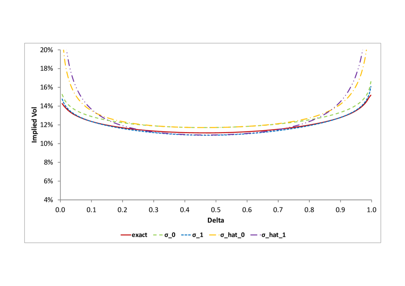
(a) T=1m

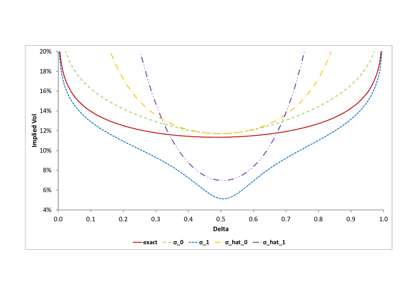
(b) T=6m

Figure 12. Comparison of the exact and asymptotic expressions for $\sigma_{imp}$ for the calibrated HSVP for different maturities. Here ”exact” denotes the exact volatility calculated by virtue of the LL formula, while $\hat{\sigma}_{\_}0$, $\hat{\sigma}_{\_}1$ and $\sigma_{\_}0$, $\sigma_{\_}1$ are given by $\hat{\sigma}_{\_}0=\hat{b}_{0}$,$\ \hat{\sigma}_{\_}1=\hat{b}_{0}+\tau\hat{b}_{1}$, and $\sigma\_0=b_{0}$,$\ \sigma_{\_}1=b_{0}+\tau b_{1}$.

9. Wing Asymptotics

9.1. General Remarks

It is well known that the high frequency asymptotics for Fourier integrals cannot be obtained in closed form unless some assumptions about smoothness or analyticity of the integrand are made. For instance, if $f\left(u\right)$ is $n$ times differentiable and decays at infinity sufficiently rapidly, one can use integration by parts and show that

$$I\left(k\right)=\int_{-\infty}^{\infty}f\left(u\right)e^{-iku}du=O\left(\left|k\right|^{-n}\right).$$

Moreover, if $f\left(u\right)$ is meromorphic only in a strip $-\mathsf{Y}_{+}<\mathop{\mathrm{I}m}u<\mathsf{Y}_{-}$, $\mathsf{Y}_{\pm}>\frac{1}{2}$, then it can be shown that

(9.1) $$I\left(k\right)\underset{k\rightarrow\pm\infty}{\sim}\Pi_{\pm}\left(k\right)+\mathsf{c}_{\pm}e^{-\mathsf{Y}_{\pm}\left|k\right|},$$

where $\Pi_{\pm}\left(k\right)$ represent contributions of the poles in the lower (upper) half-stip, respectively, and $\mathsf{c}_{\pm}$ are constants, see, e.g., [87]. Below we show how to use this result in order to calculate the wing asymptotics for the implied volatility.

9.2. Generic Exponential Lévy Processes

It is easy to apply these general results in the case of ELPs in order to calculate the wing asymptotics of the implied volatility.

Proposition 9.1.

Assume that the function $E\left(\tau,u\right)$ in the LL formula is analytical in a strip $-\mathsf{Y}_{+}<\mathop{\mathrm{I}m}\left(u\right)<\mathsf{Y}_{-}$, $\mathsf{Y}_{\pm}>\frac{1}{2}$. Then the asymptotics for the time value of a call option $\mathsf{\delta C}\left(\tau,k\right)$ has the form

(9.2) $$\mathsf{\delta C}\left(\tau,k\right)\underset{k\rightarrow\pm\infty}{\sim}\mathsf{c}_{\pm}e^{-\left(\mathsf{Y}_{\pm}\mp\frac{1}{2}\right)\left|k\right|},$$

where $\mathsf{c}_{\pm}$ are (positive) constants in (9.1). Accordingly,

(9.3) $$v_{imp}\left(\tau,k\right)\underset{k\rightarrow\pm\infty}{\sim}\beta_{\pm}\left|k\right|,\ \ \ \ \ \sigma_{imp}\left(\tau,k\right)\underset{k\rightarrow\pm\infty}{\sim}\sqrt{\frac{\beta_{\pm}\left|k\right|}{\tau}},$$

where

$$\beta_{\pm}=4\left(\mathsf{Y}_{\pm}-\sqrt{R\left(\mathsf{Y}_{\pm}\right)}\right),\ \ \ \ \ 0<\beta_{\pm}<2.$$

Proof.

See Appendix F.1.    

This result is well-known. For instance, Lee derived it by studying moment explosions, see [69]. However, its simple mathematical nature is seldom emphasized.

We can use these formulas in Proposition 9.1 to obtain expressions for $\sigma_{imp}\left(\tau,\Delta\right)$ for deep OTM ($\Delta\rightarrow 0$) and deep ITM ($\Delta\rightarrow 1$) options.

Proposition 9.2.

Assume that the assumptions of Proposition 9.1 hold. Then, in the OTM case we have

$$\sigma_{imp}\left(\tau,k\right)\underset{k\rightarrow\infty}{\sim}\sqrt{\frac{\beta_{+}k}{\tau}},$$

$$\Delta\left(\tau,k\right)\underset{k\rightarrow\infty}{\sim}\Phi\left(\left(-\frac{1-\frac{1}{2}\beta_{+}}{\sqrt{\beta_{+}}}\right)\sqrt{k}\right)\underset{k\rightarrow\infty}{\sim}\frac{\sqrt{\beta_{+}}e^{-\frac{\left(1-\beta_{+}/2\right)^{2}k}{2\beta_{+}}}}{\left(1-\beta_{+}/2\right)\sqrt{k}},$$

$$\sigma_{imp}\left(\tau,\Delta\right)\underset{\Delta\rightarrow 0}{\sim}\frac{\beta_{+}}{\left(1-\frac{1}{2}\beta_{+}\right)}\sqrt{-\frac{2\ln\left(\Delta\right)}{\tau}}.$$

Similarly, for ITM, we have

$$\sigma_{imp}\left(\tau,\Delta\right)\underset{\Delta\rightarrow 1}{\sim}\frac{\beta_{-}}{\left(1-\frac{1}{2}\beta_{-}\right)}\sqrt{-\frac{2\ln\left(1-\Delta\right)}{\tau}}.$$

Combination of these formulas yields

$$\sigma_{imp}\left(\tau,\Delta\right)\underset{\Delta\left(1-\Delta\right)\rightarrow 0}{\sim}\frac{\beta_{\mathrm{sign}\left(1/2-\Delta\right)}}{\left(1-\frac{1}{2}\beta_{\mathrm{sign}\left(1/2-\Delta\right)}\right)}\sqrt{-\frac{2\ln\left(\frac{1}{2}-\mathrm{sign}\left(1/2-\Delta\right)\left(\frac{1}{2}-\Delta\right)\right)}{\tau}}.$$

9.2.1. Specific Exponential Lévy Processes

For specific ELPs, such as TSPs, NIGPs, MPs, etc., the corresponding formulas can be made explicit.

Proposition 9.3.

For TSPs and NIGPs Proposition 9.1 holds provided that the corresponding $\mathsf{Y}_{\pm}$ are defined as follows:

$$\mathsf{Y}_{\pm} =\kappa_{\pm}\mp\frac{1}{2},\ \ \ \ \ \beta_{\pm}=\mp 2+4\left(\kappa_{\pm}-\sqrt{\kappa_{\pm}^{2}\mp\kappa_{\pm}}\right),\ \ \ TSP,$$

$$\mathsf{Y}_{\pm} =\bar{\omega},\ \ \ \ \ \beta_{\pm}=4\left(\bar{\omega}-\mathcal{\bar{\varkappa}}\right),\ \ \ \ \ NIG.$$

Thus, for NIGPs the wing volatility is symmetric. Moreover, for NIGPs the corresponding $\mathsf{c}_{\pm}$ in (9.2) have the form

$$\mathsf{c}_{\pm}=\sqrt{\frac{\bar{\omega}}{2\pi\left|k\right|^{3}}}\frac{v}{\mathcal{\bar{\varkappa}}}e^{\mathcal{\bar{\varkappa}}^{2}v}.$$

Proof.

See Appendices F.2, F.3 for details.    

The situation with MPs is somewhat different.

Proposition 9.4.

For MPs $\mathsf{Y}_{\pm}=\infty$, so that the corresponding strip of analyticity coincides with the whole axis. Accordingly, tail prices decay faster than exponential. The asymptotic behavior of the price and implied volatility for extreme strikes is given by

$$\mathsf{\delta C}^{M}\left(\tau,k\right)\underset{k\rightarrow\pm\infty}{\sim}\mathsf{c}_{\pm}\exp\left(-\frac{\sqrt{2\ln\left|k\right|}\left|k\right|}{\eta}\right),\ \ \ \ \ \sigma_{imp}\left(\tau,k\right)\underset{k\rightarrow\pm\infty}{\sim}\sqrt{\frac{\eta\left|k\right|}{2\sqrt{2\ln\left|k\right|}\tau}},$$

so that for MPs the wing volatility grows slower than linearly in absolute strike.

Proof.

See Appendix F.4 for details.    

Additional discussion is given in [99], [15], [16] and [55], [56] among others. Fast decay of the call price in the wings for MPs is in agreement with general results presented in [1].

Typical cross-sections of the corresponding volatility surfaces for $\tau=2y$ are shown in Figures 13, 14, respectively. It is clear the quality of the asymptotic approximation is far from perfect.

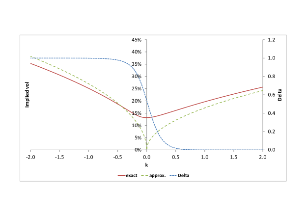
(a) TSP, $\alpha$=2/3

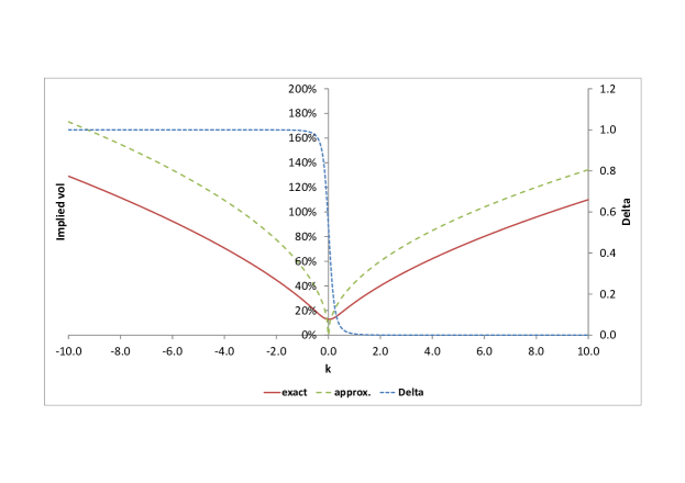
(b) TSP, $\alpha$=3/2

Figure 13. Comparison of the exact and asymptotic expressions for $\sigma_{imp}\left(k\right)$ of the calibrated TSPs for $\tau=2.0$ and $\left|k\right|\rightarrow\infty$. Here and below ”exact” denotes the exact volatility calculated by virtue of the LL formula, ”approx” denotes the approximate volatility given by (9.3), and $\Delta$ denotes the BS delta.

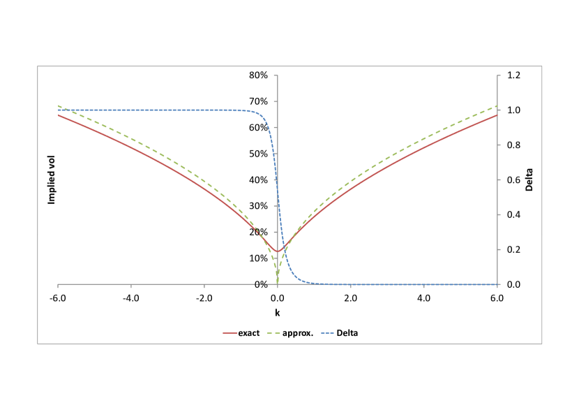
(a) NIGP

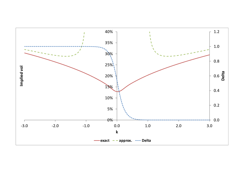
(b) MP

Figure 14. Comparison of the exact and asymptotic expressions for $\sigma_{imp}\left(k\right)$ of the calibrated NIGP and MP for $\tau=2.0$ and $\left|k\right|\rightarrow\infty$.

9.3. Quadratic Volatility Processes

Proposition 9.5.

For QVPs the asymptotic behavior of prices and implied volatility for extreme strikes is given by

$$\mathsf{\delta C}^{QV}\left(\tau,k\right)\underset{k\rightarrow\pm\infty}{\sim}\mathsf{c}_{\pm}e^{-\left(\frac{1}{2}\mp\frac{1}{2}\right)\left|k\right|},\ \ \ \ \ \sigma_{imp}\left(\tau,k\right)\underset{k\rightarrow\pm\infty}{\sim}\sqrt{\frac{2\left|k\right|}{\tau}}.$$

Proof.

See Appendix F.5.    

A typical cross-section of the volatility surface for $\tau=2y$ is shown in Figure 15(a). Once again, the quality of the asymptotic approximation is poor.

9.4. Heston Stochastic Volatility Processes

It is clear that in order to apply the general formula to HSVPs, we have to determine the analyticity strip for the function $E\left(\tau,u\right)$ given by (5.12). Analyzing the corresponding expression term by term, one can show that the corresponding strip is defined by the inequalities $-\mathsf{Y}_{+}<\mathop{\mathrm{I}m}u<\mathsf{Y}_{-}$, where $\mp\mathsf{Y}_{\pm}$ are (time-dependent) roots of the equation

$$\mathcal{F}_{-}\left(\mp i\mathsf{Y}_{\pm}\right)+\mathcal{F}_{+}\left(\mp i\mathsf{Y}_{\pm}\right)\exp\left(-\mathcal{Z}\left(\mp i\mathsf{Y}_{\pm}\right)\tau\right)=0,$$

closest to $\mp 1/2$, respectively

Proposition 9.6.

The function $E\left(\tau,u\right)$ is analytical in the strip $\mathop{\mathrm{I}m}u\in(-\mathsf{\tilde{Y}}\left(\tau\right)_{+},\mathsf{\tilde{Y}}\left(\tau\right)_{-})$, where

$$\mathsf{\tilde{Y}}_{\pm}\left(\tau\right)\geq\mathsf{Y}_{\pm}>\frac{1}{2},$$

$\mathsf{Y}_{\pm}$ are given by (7.14), and $\mp\mathsf{\tilde{Y}}_{\pm}\left(\tau\right)$ are the largest negative and the smallest positive real roots of the equation

$$\left(\rho y+\check{\kappa}\right)+\mathfrak{\varsigma}\left(y\right)+\left(-\left(\rho y+\check{\kappa}\right)+\mathfrak{\varsigma}\left(y\right)\right)e^{-\varepsilon\tau\mathfrak{\varsigma}\left(y\right)}=0,$$

where $\mathfrak{\varsigma}\left(y\right)$ is given by (7.16). The wing asymptotics of call prices and implied volatilities for HSVPs can be written as follows

$$\mathsf{\delta C}^{HSV}\left(\tau,k\right)\underset{k\rightarrow\pm\infty}{\sim}\mathsf{c}_{\pm}e^{-\left(\mathsf{\tilde{Y}}_{\pm}\left(\tau\right)\mp\frac{1}{2}\right)\left|k\right|},\ \ \ \ \ \sigma_{imp}\left(\tau,k\right)\underset{k\rightarrow\pm\infty}{\sim}\sqrt{\frac{\beta_{\pm}\left|k\right|}{\tau}},$$

where $\beta_{\pm}=4\left(\mathsf{\tilde{Y}}_{\pm}\left(\tau\right)-\sqrt{R\left(\mathsf{\tilde{Y}}_{\pm}\left(\tau\right)\right)}\right)$, $0<\beta_{\pm}<2$.

Proof.

Straightforward calculation.    

A typical cross-section of the volatility surface for $\tau=2y$ is shown in Figure 15(b). This Figure shows that the quality of wing asymptotics is satisfactory but not perfect for HSVPs.

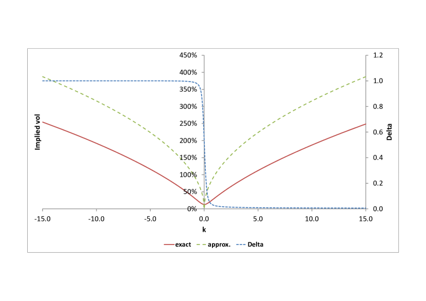
(a) QVP

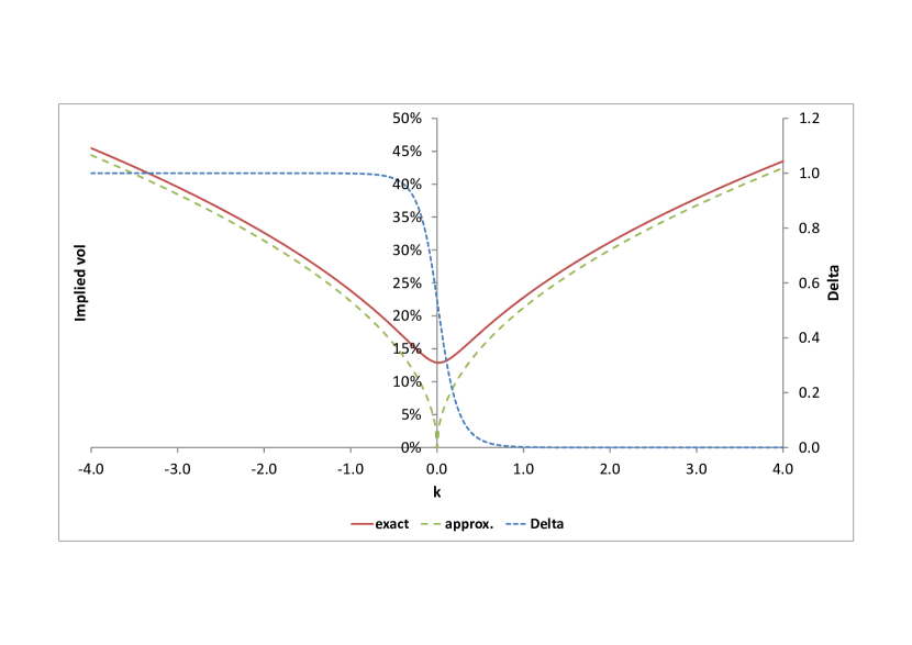
(b) HSVP

Figure 15. Comparison of the exact and asymptotic expressions for $\sigma_{imp}\left(k\right)$ of the calibrated QVP and HSVP for $\tau=2.0$ and $\left|k\right|\rightarrow\infty$.

10. Conclusions

This paper has been dedicated to the study of implied volatility asymptotics for a range of processes that allows for the use the Lewis-Lipton (LL) Fourier-integral representation of call option prices. Of key importance to us was the class of exponential Levy processes (ELPs), especially the tempered $\alpha$-stable processes, but we also discussed pure diffusion processes of the local and stochastic volatility types.

As we have demonstrated, the LL representation is highly conducive for asymptotic work, as well-established classical methods can be used to carry out examinations of large-time, large-strike, and small-time regimes – albeit occasionally with some delicacies and often involving quite laborious computations. Our work is quite complete in establishing the formulas that characterize limit behavior for volatility of the processes in question.

While some of the technical results in this paper are known, many existing results in the literature have been derived using a variety of (often complex) methods, and our paper provides a clean unification of these results along with a variety of new formulas. Generally speaking these results are theoretically appealing and provide definitive answers to a number of questions, e.g. whether non-zero limits for FX risk reversals and butterflies exist for the processes in question.

In order to establish the practical relevance for the various asymptotic results, we have taken substantial time to undertake numerical comparisons of asymptotics against the exact LL solution. The difficulty of this task should not be underestimated as the integrals in the exact LL representation become challenging to handle numerically in the various limits. Nevertheless, once the analysis is carried out, it becomes clear that the performance of the various asymptotics are definitely a mixed bag, and overall rather disappointing. For instance, it is clear that most wing (i.e. large-strike) asymptotics have domains of validity that are exceedingly small, rendering the results mostly useless in practice. The same holds for small-time asymptotics of implied volatility for ELPs, where maturities generally need to be much less than a day for the asymptotics to be accurate. On the other hand, small-time asymptotics work well for diffusion processes with local and stochastic volatility, where it is not uncommon to find that options with maturities of several years can be successfully studied in the short-time limit. This discrepancy of performance is perhaps understandable given that ELPs (with jumps) are fundamentally different from diffusions, especially when observed at small time scales.

For ELPs, what does seem to work reasonable well in many case are the long-term asymptotics where the domain of validity is often respectably large (say, covering maturities larger than one or two years). Unfortunately, this behavior is neither universal nor particularly robust, and it is not difficult to find examples of ELP configurations which, while matching the market well, result in poor long-term asymptotics. For instance, we have observed that for tempered $\alpha$-stable processes the region of validity of the long-term asymptotics is sometimes dramatically reduced when the parameter $\alpha$ is greater than one.

In summary, while ELPs are viable candidates for describing FX market dynamic, it is relatively difficult to analyze their behavior in pertinent asymptotic regimes. In order to accomplish this task successfully, one has to combine analytical and numerical methods, and even then success is not guaranteed.

Appendix A Fractional PIDEs

For $\alpha\in(0,1)$ we can rewrite the regularized integrals in  the pricing equation as follows

$$I_{\alpha,s} =\frac{\left(-s\right)^{\alpha}}{\Gamma\left(-\alpha\right)}\int_{0}^{\infty}\left(V\left(x+sy\right)-V\left(x\right)\right)\frac{e^{-\kappa_{s}y}dy}{y^{1+\alpha}}$$

$$=\frac{\left(-s\right)^{\alpha}}{\Gamma\left(-\alpha\right)}\int_{0}^{\infty}\left(e^{-\kappa_{s}y}V\left(x+sy\right)-V\left(x\right)+\left(1-e^{-\kappa_{s}y}\right)V\left(x\right)\right)\frac{dy}{y^{1+\alpha}}$$

$$=\frac{\left(-s\right)^{\alpha}}{\Gamma\left(-\alpha\right)}e^{s\kappa_{s}x}\int_{0}^{\infty}\left(\tilde{V}\left(x+sy\right)-\tilde{V}\left(x\right)\right)\frac{dy}{y^{1+\alpha}}$$

$$+\frac{\left(-s\right)^{\alpha}}{\Gamma\left(-\alpha\right)}\int_{0}^{\infty}\frac{\left(1-e^{-\kappa_{s}y}\right)dy}{y^{1+\alpha}}V\left(x\right)$$

$$=e^{s\kappa_{s}x}\mathfrak{D}_{s}^{\alpha}\left(e^{-s\kappa_{s}x}V\right)-\left(-s\right)^{\alpha}\kappa_{s}^{\alpha}V,$$

where $\tilde{V}\left(x\right)=e^{-s\kappa_{s}x}V\left(x\right)$. Similarly, for $\alpha\in(1,2)$ we have

$$I_{\alpha,s} =\frac{\left(-s\right)^{\alpha}}{\Gamma\left(-\alpha\right)}\int_{0}^{\infty}\left(V\left(x+sy\right)-V\left(x\right)-syV_{x}\left(x\right)\right)\frac{e^{-\kappa_{s}y}dy}{y^{1+\alpha}}$$

$$=\frac{\left(-s\right)^{\alpha}}{\Gamma\left(1-\alpha\right)}\int_{0}^{\infty}\left(V\left(x+sy\right)-V\left(x\right)-syV_{x}\left(x\right)\right)e^{-\kappa_{s}y}d\left(\frac{1}{y^{\alpha}}\right)$$

$$=\frac{\left(-s\right)^{\alpha}}{\Gamma\left(1-\alpha\right)}\int_{0}^{\infty}\left(-s\left(V_{x}\left(x+sy\right)-V_{x}\left(x\right)\right)+\kappa_{s}\left(V\left(x+sy\right)-V\left(x\right)-syV_{x}\left(x\right)\right)\right)\frac{e^{-\kappa_{s}y}dy}{y^{\alpha}}$$

$$=\frac{\left(-s\right)^{\alpha-1}}{\Gamma\left(1-\alpha\right)}e^{s\kappa_{s}x}\int_{0}^{\infty}\left(\tilde{V}_{x}\left(x+sy\right)-\tilde{V}_{x}\left(x\right)\right)\frac{dy}{y^{1+\left(\alpha-1\right)}}$$

$$+\frac{\left(-s\right)^{\alpha-1}}{\Gamma\left(1-\alpha\right)}\int_{0}^{\infty}\frac{\left(1-e^{-\kappa_{s}y}\right)dy}{y^{1+\left(\alpha-1\right)}}e^{s\kappa_{s}x}\tilde{V}_{x}\left(x\right)+\frac{\left(-s\right)^{\alpha-1}}{\Gamma\left(1-\alpha\right)}\kappa_{s}\int_{0}^{\infty}\frac{e^{-\kappa_{s}y}dy}{y^{\alpha-1}}V_{x}\left(x\right)$$

$$=e^{s\kappa_{s}x}\mathfrak{D}_{s}^{\alpha}\left(e^{-s\kappa_{s}x}V\right)-\left(-s\right)^{\alpha-1}\alpha\kappa_{s}^{\alpha-1}V_{x}\left(x\right)-\left(-s\right)^{\alpha}\kappa_{s}^{\alpha}V\left(x\right),$$

where $\tilde{V}\left(x\right)=e^{-s\kappa_{s}x}V\left(x\right)$. Accordingly, PIDEs (4.8), (4.9) can be written as

$$V_{t}+\gamma V_{x}+\frac{1}{2}\sigma^{2}\left(V_{xx}-V_{x}\right)+\sum\limits_{s=\pm}\left(-s\right)^{\alpha}a_{s}e^{s\kappa_{s}x}\mathfrak{D}_{s}^{\alpha}\left(e^{-s\kappa_{s}x}V\right)-\sum\limits_{s=\pm}a_{s}\kappa_{s}^{\alpha}V=0,$$

and

$$V_{t}+\left(\gamma+\sum\limits_{s=\pm}sa_{s}\alpha\kappa_{s}^{\alpha-1}\right)V_{x}+\frac{1}{2}\sigma^{2}\left(V_{xx}-V_{x}\right)+\sum\limits_{s=\pm}\left(-s\right)^{\alpha}a_{s}e^{s\kappa_{s}x}\mathfrak{D}_{s}^{\alpha}\left(e^{-s\kappa_{s}x}V\right)-\sum\limits_{s=\pm}a_{s}\kappa_{s}^{\alpha}V=0.$$

Appendix B The Green’s Function and Call Prices for Gauss-Lévy and Tempered Gauss-Lévy Processes

We start with the following assumptions: $\alpha\in(0,1)$, volatility is zero, $\sigma=0$, the process is maximally skewed to the left and there is no dumping, $c_{+}=0$, $c_{-}>0$, $\kappa_{\pm}=0$. For brevity we omit subscripts where possible. The corresponding backward and forward equations have the form

$$V_{t}+\gamma V_{x}+c\int_{0}^{\infty}\left(V\left(x-y\right)-V\left(x\right)\right)\frac{dy}{y^{1+\alpha}}=0,\ \ \ \ \ V\left(T,x\right)=V_{T}\left(x\right),$$

$$G_{t}^{\left(\alpha\right)}+\gamma G_{x}^{\left(\alpha\right)}-c\int_{0}^{\infty}\left(G^{\left(\alpha\right)}\left(x+y\right)-G^{\left(\alpha\right)}\left(x\right)\right)\frac{dy}{y^{1+\alpha}}=0,\ \ \ \ \ G^{\left(\alpha\right)}\left(0,x\right)=\delta\left(x\right).$$

where $\gamma=-a=-\Gamma\left(-\alpha\right)c=\sec\left(\alpha\pi/2\right)\vartheta^{\alpha}>0$, or, in terms of fractional derivatives,

$$V_{t}+\gamma V_{x}+a\mathfrak{D}_{-}^{\alpha}\left(V\right)=0,\ \ \ \ \ V\left(T,x\right)=V_{T}\left(x\right),$$

$$G_{t}^{\left(\alpha\right)}+\gamma G_{x}^{\left(\alpha\right)}-\left(-1\right)^{\alpha}a\mathfrak{D}_{+}^{\alpha}\left(G^{\left(\alpha\right)}\right)=0,\ \ \ \ \ G^{\left(\alpha\right)}\left(0,x\right)=\delta\left(x\right).$$

Lemma B.1.

Let $G^{\left(\alpha\right)}\left(t,x\right)$ be the Green’s function for a maximally negatively skewed stable process, such that

$$\mathrm{P}\left(X(t)\in[x,x+dx]\right)=G^{\left(\alpha\right)}\left(t,x\right).$$

Then, due to the scaling invariance of the corresponding process, we have

$$G^{\left(\alpha\right)}\left(t,x\right)=\frac{1}{\iota^{1/\alpha}}g^{\left(\alpha\right)}\left(\xi\right),$$

where

$$\iota=\sec\left(\frac{\alpha\pi}{2}\right)\vartheta^{\alpha}t,\ \ \ \xi=\frac{\left(x-\iota\right)}{\iota^{1/\alpha}},$$

and $g^{\left(\alpha\right)}\left(.\right)$ is an appropriate positive function of a single variable, which satisfies the following ordinary integro-differential equation

(B.1) $$\xi g^{\left(\alpha\right)}\left(\xi\right)+\frac{1}{\Gamma\left(1-\alpha\right)}\int_{0}^{\infty}g^{\left(\alpha\right)}\left(\xi+\xi^{\prime}\right)\frac{d\xi^{\prime}}{\xi^{\prime\alpha}}=0.$$

In particular, the Green’s function associated with the LGP has the form

(B.2) $$G^{\left(1/2\right)}\left(t,x\right)=\frac{1}{\iota^{2}}g^{\left(1/2\right)}\left(\xi\right),$$

where

$$\iota=\sqrt{2\vartheta}t,\ \ \ \xi=\frac{\left(x-\iota\right)}{\iota^{2}},\ \ \ g^{\left(1/2\right)}\left(\xi\right)=\frac{\exp\left(\frac{1}{4\xi}\right)}{2\sqrt{\pi}\left(-\xi\right)^{3/2}}\mathbf{1}_{\xi<0}.$$

This density is known as the Lévy distribution.

Proof.

In order to calculate $G^{\left(\alpha\right)}$ we use the following ansatz

$$G^{\left(\alpha\right)}\left(t,x\right)=\frac{1}{\iota^{\alpha^{\prime}}}g^{\left(\alpha\right)}\left(\frac{x-\iota}{\iota^{\alpha^{\prime}}}\right),$$

where $\iota=\gamma t$, and $\alpha^{\prime}=1/\alpha$. Its validity is verified below. Since

$$\int_{-\infty}^{\infty}G^{\left(\alpha\right)}\left(t,x\right)dx=\int_{-\infty}^{\infty}g^{\left(\alpha\right)}\left(\frac{x-\iota}{\iota^{\alpha^{\prime}}}\right)d\left(\frac{x-\iota}{\iota^{\alpha^{\prime}}}\right)=\int_{-\infty}^{\infty}g^{\left(\alpha\right)}\left(\xi\right)d\xi,$$

we have to impose the following constraints on $g$:

(B.3) $$g^{\left(\alpha\right)}\left(\xi\right)\geq 0,\ \ \ \ \ g^{\left(\alpha\right)}\left(\xi\right)\underset{\xi\rightarrow\pm\infty}{\rightarrow}0,\ \ \ \ \ \int_{-\infty}^{\infty}g^{\left(\alpha\right)}\left(\xi\right)d\xi=1,$$

which, broadly speaking, play the role of initial and boundary conditions. We have

$$0 =G_{t}^{\left(\alpha\right)}\left(t,x\right)+\gamma G_{x}^{\left(\alpha\right)}\left(t,x\right)-\left(-1\right)^{\alpha}a\mathfrak{D}_{+}^{\alpha}G^{\left(\alpha\right)}\left(t,x\right)$$

$$=-\frac{\alpha^{\prime}\gamma}{\iota^{\alpha^{\prime}+1}}\left(\xi g_{\xi}^{\left(\alpha\right)}\left(\xi\right)+g^{\left(\alpha\right)}\left(\xi\right)\right)-\frac{\left(-1\right)^{\alpha}}{\iota^{\alpha^{\prime}+\alpha\alpha^{\prime}}}a\mathfrak{D}_{+}^{\alpha}g^{\left(\alpha\right)}\left(\xi\right).$$

It is clear that $t$-dependence disappears and the integro-differential equation for $g\left(\xi\right)$ becomes

(B.4) $$\xi g_{\xi}^{\left(\alpha\right)}\left(\xi\right)+g^{\left(\alpha\right)}\left(\xi\right)+\left(-1\right)^{\alpha}\alpha\mathfrak{D}_{+}^{\alpha}g^{\left(\alpha\right)}\left(\xi\right)=0.$$

Here $-\infty<\xi<0$. If so desired, we can manipulate this equation further. Specifically, we can integrate by parts and write

$$\left(\xi g^{\left(\alpha\right)}\left(\xi\right)\right)_{\xi}+\frac{1}{\Gamma\left(1-\alpha\right)}\int_{0}^{\infty}g_{\xi}^{\left(\alpha\right)}\left(\xi+\xi^{\prime}\right)\frac{d\xi^{\prime}}{\xi^{\prime\alpha}}=0,$$

or, after integration over the interval $\left(-\infty,\xi\right]$,

$$\xi g^{\left(\alpha\right)}\left(\xi\right)+\frac{1}{\Gamma\left(1-\alpha\right)}\int_{0}^{\infty}g^{\left(\alpha\right)}\left(\xi+\xi^{\prime}\right)\frac{d\xi^{\prime}}{\xi^{\prime\alpha}}=0,$$

which is (B.1). In particular, it is easy to check directly that for the LGPs with $\alpha=1/2$, $c_{+}=0$, $c_{-}=\sqrt{2\vartheta}$, the corresponding $g^{\left(1/2\right)}$ is given by (B.2). The case of $\alpha\in\left(1,2\right)$ can be studied in a similar fashion.    

It is clear that our calculations make sense by virtue of the fact that the corresponding maximally skewed stable processes are scale-invariant. Since two-sided stable processes possess this property as well, the above calculations can be repeated verbatim for such processes. It can be shown that the PDFs of standard stable laws have the following support: (A) the positive semi-axis if $\alpha\in\left(0,1\right),\ c_{-}=0$; (B) the negative semi-axis if $\alpha\in\left(0,1\right),\ c_{+}=0$; (C) the whole axis in all other cases. If $\alpha\in\left(0,2\right)$, $c_{+}>0$, $c_{-}\geq 0$, then for $\xi\rightarrow\infty$ we have

$$g^{\left(\alpha\right)}\left(\left.\xi\right|\alpha,\beta\right)\sim\xi^{-\left(\alpha+1\right)}.$$

If $\alpha\in\left(0,2\right)$, $c_{+}\geq 0$, $c_{-}>0$, then for $\xi\rightarrow-\infty$ we have

$$g^{\left(\alpha\right)}\left(\left.\xi\right|\alpha,\beta\right)\sim\left|\xi\right|^{-\left(\alpha+1\right)}.$$

Thus, for all $\alpha\in\left(0,2\right)$, $c_{+}>0$, $c_{-}>0$, both tails are described by power laws. If $c_{-}=0$ $\left(c_{+}=0\right)$, then the left (right) tail is described by an exponential law.

It is clear that appropriately transformed tempered stable density is not scale-invariant unless it is maximally skewed. Because of that, we only deal with maximally skewed TSPs. Thus, we assume that $\alpha\in(0,1)$, $\sigma=0$, $c_{-}>0$, $\kappa_{-}>0$, and $c_{+}=0$. For brevity, we omit subscripts. In this case, backward equation (4.8) simplifies to the form

$$V_{t}+\gamma V_{x}+c\int_{0}^{\infty}\left(V\left(x-y\right)-V\left(x\right)\right)\frac{e^{-\kappa y}dy}{y^{1+\alpha}}=0,$$

where $\gamma=-$$\zeta$$a=-\Gamma\left(-\alpha\right)\zeta c>0$, $\mathsf{\zeta}=\left(\kappa+1\right)^{\alpha}-\kappa^{\alpha}$. The corresponding adjoint equation for the Green’s function $G^{\left(\alpha,\kappa\right)}\left(t,x\right)$ is

$$G_{t}^{\left(\alpha,\kappa\right)}+\gamma G_{x}^{\left(\alpha,\kappa\right)}-c\int_{0}^{\infty}\left(G^{\left(\alpha,\kappa\right)}\left(x+y\right)-G^{\left(\alpha,\kappa\right)}\left(x\right)\right)\frac{e^{-\kappa y}dy}{y^{1+\alpha}}=0.$$

Equivalently, the backward and forward equations can be written in terms of fractional derivatives as follows

$$V_{t}+\gamma V_{x}+ae^{-\kappa x}\mathfrak{D}_{-}^{\alpha}\left(e^{\kappa x}V\right)+\delta V=0,\ \ \ \ \ V\left(T,x\right)=v\left(x\right),$$

(B.5) $$G_{t}^{\left(\alpha,\kappa\right)}+\gamma G_{x}^{\left(\alpha,\kappa\right)}-\left(-1\right)^{\alpha}ae^{\kappa x}\mathfrak{D}_{+}^{\alpha}\left(e^{-\kappa x}G^{\left(\alpha,\kappa\right)}\right)-\delta G^{\left(\alpha,\kappa\right)}=0,\ \ \ \ \ G^{\left(\alpha\right)}\left(0,x\right)=\delta\left(x\right),$$

where $\delta\mathcal{=}-\kappa^{\alpha}a=-\Gamma\left(-\alpha\right)\kappa^{\alpha}c>0$. It turns out that for a maximally skewed TSP can be converted into a maximally skewed SP via a simple scaling transformation.

Lemma B.2.

Let $G^{\left(\alpha,\kappa\right)}\left(t,x\right)$ be the Green’s function for a maximally negatively skewed tempered stable process. Then

(B.6) $$G^{\left(\alpha,\kappa\right)}\left(t,x\right)=\frac{\exp\left(\iota_{1}+\kappa\left(x-\left(\iota_{2}-\iota_{1}\right)\right)\right)}{\iota^{1/\alpha}}g^{\left(\alpha\right)}\left(\xi\right),$$

where

$$\iota=\sec\left(\frac{\alpha\pi}{2}\right)\vartheta^{\alpha}t,\ \ \ \iota_{1}=\kappa^{\alpha}\iota,\ \ \ \iota_{2}=\left(\kappa+1\right)^{\alpha}\iota,\ \ \ \xi=\frac{\left(x-\left(\iota_{2}-\iota_{1}\right)\right)}{\iota^{1/\alpha}}.$$

In particular, for $\alpha=1/2$ we have

(B.7) $$G^{\left(1/2,\kappa\right)}\left(t,x\right)=\frac{\exp\left(\iota_{1}+\kappa\left(x-\left(\iota_{2}-\iota_{1}\right)\right)\right)}{\iota^{2}}g^{\left(1/2\right)}\left(\xi\right),$$

where

$$\iota=\sqrt{2\vartheta}t,\ \ \ \iota_{1}=\sqrt{\kappa}\iota,,\ \ \ \iota_{2}=\sqrt{\kappa+1}\iota,\ \ \ \xi=\frac{\left(x-\left(\iota_{2}-\iota_{1}\right)\right)}{\iota^{2}}.$$

Proof.

After some tedious algebra it can be show that solution of (B.5) can be written in the form

$$G^{\left(\alpha,\kappa\right)}\left(t,x\right)=\mathsf{\zeta}^{-\frac{1}{\left(1-\alpha\right)}}e^{\kappa^{\alpha}\iota+\kappa\left(x-\zeta\iota\right)}G^{\left(\alpha\right)}\left(\mathsf{\zeta}^{-\frac{\alpha}{\left(1-\alpha\right)}}\iota,\mathsf{\zeta}^{-\frac{1}{\left(1-\alpha\right)}}x\right).$$

Accordingly, we can represent $G^{\left(\alpha,\kappa\right)}\left(t,x\right)$ as follows

$$G^{\left(\alpha,\kappa\right)}\left(t,x\right)=\frac{e^{\kappa^{\alpha}\iota+\kappa\left(x-\zeta\iota\right)}}{\iota^{1/\alpha}}g^{\left(\alpha\right)}\left(\frac{x-\zeta\iota}{\iota^{1/\alpha}}\right),$$

where $g^{\left(\alpha\right)}$ satisfies (B.1) subject to (B.3). In particular, for the TLGPs we have (B.7).    

Next, we consider prices of options for maximally skewed stable and tempered stable process via the Esscher transform technique (see, e.g., [54]). Due to the strong localization of the corresponding Green’s function, we can define its Esscher transform as follows

$$g^{\left(\alpha\right)}\left(\xi\right)\Rightarrow g^{\left(\alpha,p\right)}\left(\xi\right)=\frac{e^{p\xi}g^{\left(\alpha\right)}\left(\xi\right)}{\mathbb{E}\left\{e^{p\xi}g^{\left(\alpha\right)}\left(\xi\right)\right\}}=e^{p\xi-\psi\left(-ip\right)}g^{\left(\alpha\right)}\left(\xi\right),$$

As usual, we denote the corresponding complementary cumulative function as

$$\Gamma^{\left(\alpha,p\right)}\left(\xi\right)=\int_{\xi}^{\infty}g^{\left(\alpha,p\right)}\left(\xi^{\prime}\right)d\xi^{\prime}.$$

With this notation in mind, we can write the price of a call option on a maximally skewed SP as follows

$$\mathsf{C}\left(\iota,k\right) =\int_{k}^{\infty}\left(e^{x}-e^{k}\right)\frac{1}{\iota^{1/\alpha}}g^{\left(\alpha\right)}\left(\frac{x-\iota}{\iota^{1/\alpha}}\right)dx$$

$$=\int_{\frac{k-\iota}{\iota^{1/\alpha}}}^{\infty}\left(e^{\iota+\iota^{1/\alpha}\xi}-e^{\kappa}\right)g^{\left(\alpha\right)}\left(\xi\right)d\xi$$

$$=e^{\iota+\psi\left(-i\iota^{1/\alpha}\right)}\Gamma^{\left(\alpha,\iota^{1/\alpha}\right)}\left(\frac{k-\iota}{\iota^{1/\alpha}}\right)-e^{k}\Gamma^{\left(\alpha,0\right)}\left(\frac{k-\iota}{\iota^{1/\alpha}}\right).$$

In particular, for the LGP, assuming that $k<\iota$, we can represent the normalized price of a call option as follows

$$\mathsf{C}\left(\iota,k\right) =\frac{\iota}{2\sqrt{\pi}}\int_{k}^{\iota}\left(e^{x}-e^{k}\right)\frac{e^{-\frac{\iota^{2}}{4(\iota-x)}}}{\left(\iota-x\right)^{3/2}}dx$$

$$=\frac{1}{2\sqrt{\pi}}\int_{\frac{k-\iota}{\iota^{2}}}^{0}\left(e^{\iota+\iota^{2}\xi}-e^{k}\right)\frac{e^{\frac{1}{4\xi}}}{\left(-\xi\right)^{3/2}}d\xi$$

$$=e^{\iota}\mathsf{D}\left(v,2\iota\right)-e^{k}\mathsf{D}\left(v,0\right),$$

where $v=2\iota^{2}/\left(\iota-k\right)$. In order to compute the corresponding integrals explicitly, we use the change of variables $\xi=-1/2z^{2}$. For maximally skewed TLGP we can represent the price of a call option as follows

$$\mathsf{C}\left(\iota,k\right) =\frac{\iota}{2\sqrt{\pi}}\int_{k}^{\iota_{2}-\iota_{1}}\left(e^{x}-e^{k}\right)\frac{e^{\iota_{1}+\kappa\left(x-\left(\iota_{2}-\iota_{1}\right)\right)-\frac{\iota^{2}}{4(\left(\iota_{2}-\iota_{1}\right)-x)}}}{\left(\iota_{2}-\iota_{1}-x\right)^{3/2}}dx$$

$$=\frac{e^{\iota_{1}}}{2\sqrt{\pi}}\int_{\frac{k-\left(\iota_{2}-\iota_{1}\right)}{\iota^{2}}}^{0}\left(e^{\iota_{2}-\iota_{1}-\iota^{2}\xi}-e^{k}\right)\frac{e^{\kappa\iota^{2}\xi+\frac{1}{4\xi}}}{\left(-\xi\right)^{3/2}}d\xi$$

$$=e^{\iota_{2}}\mathsf{D}\left(v,2\iota_{2}\right)-e^{k+\iota_{1}}\mathsf{D}\left(v,2\iota_{1}\right),$$

where $v=2\iota^{2}/\left(\iota_{2}-\iota_{1}-k\right)$.

Appendix C The Implied Volatility Expansion

By definition,

$$\mathsf{C}\left(\tau,k\right) =\Phi\left(-\frac{k}{\bar{\sigma}_{imp}}+\frac{\bar{\sigma}_{imp}}{2}\right)-e^{k}\Phi\left(-\frac{k}{\bar{\sigma}_{imp}}-\frac{\bar{\sigma}_{imp}}{2}\right),$$

$$\mathsf{C}_{k}\left(\tau,k\right) =\phi\left(-\frac{k}{\bar{\sigma}_{imp}}+\frac{\bar{\sigma}_{imp}}{2}\right)\partial_{k}\bar{\sigma}_{imp}-e^{k}\Phi\left(-\frac{k}{\bar{\sigma}_{imp}}-\frac{\bar{\sigma}_{imp}}{2}\right),$$

$$\mathsf{C}_{kk}\left(\tau,k\right) =\phi\left(-\frac{k}{\bar{\sigma}_{imp}}+\frac{\bar{\sigma}_{imp}}{2}\right)\left(\partial_{k}^{2}\bar{\sigma}_{imp}+\partial_{k}\bar{\sigma}_{imp}-\frac{\bar{\sigma}_{imp}\left(\partial_{k}\bar{\sigma}_{imp}\right)^{2}}{4}\right.$$

$$\left.+\frac{1}{\bar{\sigma}_{imp}}+\frac{k^{2}\left(\partial_{k}\bar{\sigma}_{imp}\right)^{2}}{\bar{\sigma}_{imp}^{3}}-\frac{2k\partial_{k}\bar{\sigma}_{imp}}{\bar{\sigma}_{imp}^{2}}\right)-e^{k}\Phi\left(-\frac{k}{\bar{\sigma}_{imp}}-\frac{\bar{\sigma}_{imp}}{2}\right).$$

For $k=0$ we have

(C.1) $$\mathsf{C}\left(\tau,0\right)=\Phi\left(\frac{\bar{\chi}_{0}\left(\tau\right)}{2}\right)-\Phi\left(-\frac{\bar{\chi}_{0}\left(\tau\right)}{2}\right)\sim\frac{1}{\sqrt{2\pi}}\left(1-\frac{\bar{\chi}_{0}^{2}\left(\tau\right)}{24}\right)\bar{\chi}_{0}\left(\tau\right),$$

(C.2) $$\mathsf{C}_{k}\left(\tau,0\right) =\phi\left(\frac{\bar{\chi}_{0}\left(\tau\right)}{2}\right)\bar{\chi}_{1}\left(\tau\right)-\Phi\left(-\frac{\bar{\chi}_{0}\left(\tau\right)}{2}\right)$$

$$\sim\frac{1}{\sqrt{2\pi}}\left(1-\frac{\bar{\chi}_{0}^{2}\left(\tau\right)}{8}\right)\bar{\chi}_{1}\left(\tau\right)+\frac{1}{2}\left(\mathsf{C}\left(\tau,0\right)-1\right),$$

(C.3) $$\mathsf{C}_{kk}\left(\tau,0\right) =\phi\left(\frac{\bar{\chi}_{0}\left(\tau\right)}{2}\right)\left(\bar{\chi}_{2}\left(\tau\right)+\bar{\chi}_{1}\left(\tau\right)-\frac{1}{4}\bar{\chi}_{0}\left(\tau\right)\bar{\chi}_{1}^{2}\left(\tau\right)+\frac{1}{\bar{\chi}_{0}\left(\tau\right)}\right)-\Phi\left(-\frac{\bar{\chi}_{0}\left(\tau\right)}{2}\right)$$

$$\sim\frac{1}{\sqrt{2\pi}}\left(1-\frac{\bar{\chi}_{0}^{2}\left(\tau\right)}{8}\right)\left(\bar{\chi}_{2}\left(\tau\right)-\frac{1}{4}\bar{\chi}_{0}\left(\tau\right)\bar{\chi}_{1}^{2}\left(\tau\right)+\frac{1}{\bar{\chi}_{0}\left(\tau\right)}\right)+\mathsf{C}_{k}\left(\tau,0\right).$$

Comparison of (8.2), (C.1) - (C.3) yields

$$\left(1-\frac{\bar{\chi}_{0}^{2}\left(\tau\right)}{24}\right)\bar{\chi}_{0}\left(\tau\right)=\mathfrak{\hat{l}}\left(\tau\right),$$

$$\left(1-\frac{\bar{\chi}_{0}^{2}\left(\tau\right)}{8}\right)\bar{\chi}_{1}\left(\tau\right)=\mathfrak{\hat{m}}\left(\tau\right),$$

$$\left(1-\frac{\bar{\chi}_{0}^{2}\left(\tau\right)}{8}\right)\left(\bar{\chi}_{2}\left(\tau\right)-\frac{1}{4}\bar{\chi}_{0}\left(\tau\right)\bar{\chi}_{1}^{2}\left(\tau\right)+\frac{1}{\bar{\chi}_{0}\left(\tau\right)}\right)=\mathfrak{\hat{n}}\left(\tau\right),$$

$$\bar{\chi}_{0}\left(\tau\right)\sim\mathfrak{\hat{l}}\left(\tau\right)\left(1+\frac{\mathfrak{\hat{l}}^{2}\left(\tau\right)}{24}\right),$$

$$\bar{\chi}_{1}\left(\tau\right)\sim\mathfrak{\hat{m}}\left(\tau\right)\left(1+\frac{\mathfrak{\hat{l}}^{2}\left(\tau\right)}{8}\right),$$

$$\bar{\chi}_{2}\left(\tau\right)\sim-\frac{1}{\mathfrak{\hat{l}}\left(\tau\right)}+\frac{\mathfrak{\hat{l}}\left(\tau\right)}{24}+\frac{1}{4}\mathfrak{\hat{l}}\left(\tau\right)\mathfrak{\hat{m}}^{2}\left(\tau\right)+\mathfrak{\hat{n}}\left(\tau\right)\left(1+\frac{\mathfrak{\hat{l}}^{2}\left(\tau\right)}{8}\right).$$

Noticing that $\bar{\chi}_{i}\left(\tau\right)=\chi_{i}\left(\tau\right)\tau^{1/2}$, we obtain the result.

Appendix D Long-time Asymptotics

D.1. Exponential Lévy Processes

Due to the fact that we have chosen a parametric representation of $\bar{k}$ in terms of $y$, so that we know that the saddlepoint is located on the imaginary axis at $u=iy$, it is easy to perform the corresponding saddlepoint calculation. When $-\frac{1}{2}<y<\frac{1}{2}$, we can perform parallel move of the contour of integration to a new contour given by the equation

$$\mathop{\mathrm{I}m}u=y,$$

without hitting singularities located at $u=\pm i/2$. Accordingly, we can approximate the price of the call option as follows

(D.1) $$\mathsf{C}\left(\tau,\bar{k}\left(y\right)\tau\right)=1+\frac{1}{\sqrt{2\pi\tau}}e^{\tau\Xi_{01}^{\left(+\right)}\left(y\right)}c_{0}\left(y\right)\left(1-\frac{1}{\tau}c_{1}\left(y\right)\right).$$

When $-\kappa_{+}+\frac{1}{2}<y<-\frac{1}{2}$ or $\frac{1}{2}<y<\kappa_{-}+\frac{1}{2}$, in the process of moving the contour of integration, we shall hit the points $u=-i/2$ and $i/2$, respectively. We note that

$$S_{+}=S\left(\frac{i}{2}\right)=\bar{k},\ \ \ S_{-}=S\left(-\frac{i}{2}\right)=a_{+}\left(\kappa_{+}-1\right)^{\alpha}+a_{-}\left(\kappa_{-}+1\right)^{\alpha}+\gamma+\delta=0,$$

so that, by virtue of the Cauchy theorem, the corresponding approximate prices can be written as

(D.2) $$\mathsf{C}\left(\tau,\bar{k}\left(y\right)\tau\right)=\left\{\begin{array}[]{ll}1-e^{\bar{k}\left(y\right)\tau}+\frac{1}{\sqrt{2\pi\tau}}e^{\tau\Xi_{01}^{\left(+\right)}\left(y\right)}c_{0}\left(y\right)\left(1-\frac{1}{\tau}c_{1}\left(y\right)\right),&\frac{1}{2}<y<\kappa_{-}+\frac{1}{2},\\ \frac{1}{\sqrt{2\pi\tau}}e^{\tau\Xi_{01}^{\left(+\right)}\left(y\right)}c_{0}\left(y\right)\left(1-\frac{1}{\tau}c_{1}\left(y\right)\right),&-\kappa_{+}+\frac{1}{2}<y<-\frac{1}{2}.\end{array}\right.$$

Comparison on expressions (D.1), (D.2) and (6.6) immediately yields (7.7).

Consider $y\in\left(-\mathsf{Y}_{+},\mathsf{Y}_{-}\right)$ and define

(D.3) $$\Xi_{2}\left(y\right)=\Xi_{0}^{\prime\prime}\left(y\right),\ \ \ \Xi_{3}\left(y\right)=\Xi_{0}^{\prime\prime\prime}\left(y\right),\ \ \ \Xi_{4}\left(y\right)=\Xi_{0}^{\prime\prime\prime\prime}\left(y\right),$$

(D.4) $$f_{0}\left(y\right)=\frac{1}{R\left(y\right)},\ \ \ f_{1}\left(y\right)=f_{0}^{\prime}\left(y\right)=-\frac{2y}{\left(R\left(y\right)\right)^{2}},\ \ \ f_{2}\left(y\right)=f_{0}^{\prime\prime}\left(y\right)=\frac{\left(6y^{2}+\frac{1}{2}\right)}{\left(R\left(y\right)\right)^{3}},$$

(D.5) $$c_{0}\left(y\right) =\frac{f_{0}\left(y\right)}{\sqrt{\Xi_{2}\left(y\right)}}=\frac{1}{\sqrt{\Xi_{2}\left(y\right)}R\left(y\right)},$$

$$c_{1}\left(y\right) =-\frac{1}{2\Xi_{2}\left(y\right)}\left(\frac{f_{2}\left(y\right)}{f_{0}\left(y\right)}-\frac{\Xi_{3}\left(y\right)f_{1}\left(y\right)}{\Xi_{2}\left(y\right)f_{0}\left(y\right)}+\frac{5\Xi_{3}^{2}\left(y\right)}{12\Xi_{2}^{2}\left(y\right)}-\frac{\Xi_{4}\left(y\right)}{4\Xi_{2}\left(y\right)}\right)$$

$$-\frac{1}{2\Xi_{2}\left(y\right)}\left(\frac{\left(6y^{2}+\frac{1}{2}\right)}{\left(R\left(y\right)\right)^{2}}+\frac{2y\Xi_{3}\left(y\right)}{R\left(y\right)\Xi_{2}\left(y\right)}+\frac{5\Xi_{3}^{2}\left(y\right)}{12\Xi_{2}^{2}\left(y\right)}-\frac{\Xi_{4}\left(y\right)}{4\Xi_{2}\left(y\right)}\right),$$

(D.6) $$a_{0}\left(y\right) =2\left(s_{+}\left(y\right)-s_{-}\left(y\right)\right)^{2},$$

$$a_{1}\left(y\right) =\frac{2\ln\left(a_{0}^{1/2}\left(y\right)r\left(y\right)c_{0}\left(y\right)\right)}{r\left(y\right)},$$

$$a_{2}\left(y\right) =\frac{2c_{1}\left(y\right)}{r\left(y\right)}$$

$$+\frac{\left(r\left(y\right)a_{1}\left(y\right)\left(\left(r\left(y\right)a_{1}\left(y\right)-3\right)\left(r\left(y\right)+\frac{1}{4}\right)-\frac{1}{4}\right)+6r\left(y\right)+2\right)}{r^{3}\left(y\right)a_{0}\left(y\right)},$$

(D.7) $$b_{0}\left(y\right)=a_{0}^{1/2}\left(y\right),\ \ \ b_{1}\left(y\right)=\frac{a_{1}\left(y\right)}{2a_{0}^{1/2}\left(y\right)},\ \ \ b_{2}\left(y\right)=\frac{4a_{0}\left(y\right)a_{2}\left(y\right)-a_{1}^{2}\left(y\right)}{8a_{0}^{3/2}\left(y\right)},$$

where

(D.8) $$s_{\pm}\left(y\right)=\mathrm{sign}\left(y\pm\frac{1}{2}\right)\sqrt{-\Xi_{01,\pm}\left(y\right)},\ \ \ r\left(y\right)=R\left(\frac{\Xi_{1}\left(y\right)}{a_{0}\left(y\right)}\right).$$

D.2. Tempered Stable Processes

For completeness we present explicit formulas for $\Xi_{i}$:

$$\Xi_{0}\left(y\right) =\frac{1}{2}\sigma^{2}\left(y^{2}-\frac{1}{4}\right)+\sum_{s=\pm}a_{s}\left(\kappa_{s}+s\left(y-\frac{1}{2}\right)\right)^{\alpha}-\gamma\left(y-\frac{1}{2}\right)+\delta,$$

$$\Xi_{1}\left(y\right) =\sigma^{2}y+\alpha\sum_{s=\pm}sa_{s}\left(\kappa_{s}+s\left(y-\frac{1}{2}\right)\right)^{\alpha-1}-\gamma,$$

$$\Xi_{2}\left(y\right) =\sigma^{2}+\alpha\left(\alpha-1\right)\sum_{s=\pm}a_{s}\left(\kappa_{s}+s\left(y-\frac{1}{2}\right)\right)^{\alpha-2},$$

$$\Xi_{3}\left(y\right) =\alpha\left(\alpha-1\right)\left(\alpha-2\right)\sum_{s=\pm}sa_{s}\left(\kappa_{s}+s\left(y-\frac{1}{2}\right)\right)^{\alpha-3},$$

$$\Xi_{4}\left(y\right) =\alpha\left(\alpha-1\right)\left(\alpha-2\right)\left(\alpha-3\right)\sum_{s=\pm}a_{s}\left(\kappa_{s}+s\left(y-\frac{1}{2}\right)\right)^{\alpha-4}.$$

D.3. Normal Inverse Gaussian Processes

For completeness, we present explicit expressions for $\Xi_{i}$:

$$\Xi_{0}\left(y\right) =\sigma^{2}\mathcal{\bar{\varkappa}}\left(\mathcal{\bar{\varkappa}}-\Lambda\left(y\right)\right),$$

$$\Xi_{1}\left(y\right) =\sigma^{2}\mathcal{\bar{\varkappa}}y\Lambda^{-1}\left(y\right),$$

$$\Xi_{2}\left(y\right) =\sigma^{2}\mathcal{\bar{\varkappa}\omega}^{2}\Lambda^{-3}\left(y\right),$$

$$\Xi_{3}\left(y\right) =3\sigma^{2}\mathcal{\bar{\varkappa}\omega}^{2}y\Lambda^{-5}\left(y\right),$$

$$\Xi_{4}\left(y\right) =3\sigma^{2}\mathcal{\bar{\varkappa}\omega}^{2}\left(\mathcal{\omega}^{2}+4y^{2}\right)\Lambda^{-7}\left(y\right),$$

where $\Lambda\left(y\right)=\sqrt{\mathcal{\bar{\omega}}^{2}-y^{2}}$.

By using (4.18), we can calculate long-time asymptotics for call prices directly. For  $k=\hat{k}v$ and $v\rightarrow\infty$, where $v=\sigma^{2}\tau$, we have

$$\mathsf{C}^{NIG}\left(v,\hat{k}v\right) =\frac{\bar{\omega}\mathcal{\bar{\varkappa}}ve^{\mathcal{\bar{\varkappa}}^{2}v}}{\pi}\int_{\hat{k}v}^{\infty}\frac{\left(e^{\frac{x}{2}}-e^{\hat{k}v-\frac{x}{2}}\right)K_{1}\left(\bar{\omega}\sqrt{x^{2}+\mathcal{\bar{\varkappa}}^{2}v^{2}}\right)}{\sqrt{x^{2}+\mathcal{\bar{\varkappa}}^{2}v^{2}}}dx$$

$$=1-\frac{\bar{\omega}\mathcal{\bar{\varkappa}}ve^{\mathcal{\bar{\varkappa}}^{2}v}}{\pi}\left(\int_{-\frac{\hat{k}}{2\mathcal{\bar{\varkappa}}}}^{\infty}\frac{e^{-\mathcal{\bar{\varkappa}}vy}K_{1}\left(2\bar{\omega}\mathcal{\bar{\varkappa}}vQ^{1/2}\left(y\right)\right)}{Q^{1/2}\left(y\right)}dy\right.$$

$$\left.+\int_{\frac{\hat{k}}{2\mathcal{\bar{\varkappa}}}}^{\infty}\frac{e^{\hat{k}v-\mathcal{\bar{\varkappa}}vy}K_{1}\left(2\bar{\omega}\mathcal{\bar{\varkappa}}vQ^{1/2}\left(y\right)\right)}{Q^{1/2}\left(y\right)}dy\right)$$

$$\sim 1-\sqrt{\frac{\bar{\omega}\mathcal{\bar{\varkappa}}v}{4\pi}}e^{\mathcal{\bar{\varkappa}}^{2}v}\left(\int_{-\frac{\hat{k}}{2\mathcal{\bar{\varkappa}}}}^{\infty}\frac{e^{-\mathcal{\bar{\varkappa}}v\left(y+2\bar{\omega}Q^{1/2}\left(y\right)\right)}}{Q^{3/4}\left(y\right)}\left(1+\frac{3}{16\bar{\omega}\mathcal{\bar{\varkappa}}vQ^{1/2}\left(y\right)}\right)dy\right.$$

$$\left.+e^{\hat{k}v}\int_{\frac{\hat{k}}{2\mathcal{\bar{\varkappa}}}}^{\infty}\frac{e^{-\mathcal{\bar{\varkappa}}v\left(y+2\bar{\omega}Q^{1/2}\left(y\right)\right)}}{Q^{3/4}\left(y\right)}\left(1+\frac{3}{16\bar{\omega}\mathcal{\bar{\varkappa}}\bar{\tau}Q^{1/2}\left(y\right)}\right)dy\right),$$

where $x=\pm 2\mathcal{\bar{\varkappa}}vy$. Consider the following function

$$\Sigma\left(y\right)=\mathcal{\bar{\varkappa}}\left(y+2\bar{\omega}Q^{1/2}\left(y\right)\right).$$

It is easy to show that on the real axis this function has a unique global minimum $y_{\ast}$ such that

$$y_{\ast}=-\frac{1}{4\mathcal{\bar{\varkappa}}},\ \ \ \ \ \Sigma_{\ast}=\Sigma\left(y_{\ast}\right)=\mathcal{\bar{\varkappa}}^{2}.$$

Assuming for brevity that $\left|\hat{k}\right|<1/2$, so that this point lies outside the domain of integration for both integrals in the above expression, we can use the original Laplace method to evaluate these integrals asymptotically and get

$$\mathsf{C}\left(v,\hat{k}v\right) \sim 1+\sqrt{\frac{\bar{\omega}}{\pi\mathcal{\bar{\varkappa}}v}}e^{\mathcal{\bar{\varkappa}}v\left(\mathcal{\bar{\varkappa}}+\frac{\hat{k}}{2\mathcal{\bar{\varkappa}}}-2\bar{\omega}\hat{Q}^{1/2}\right)}\frac{\hat{Q}^{1/4}}{R\left(\hat{k}\right)}$$

$$\times\left(1-\frac{1}{\mathcal{\bar{\varkappa}}v}\left(\frac{3\bar{\omega}\hat{k}^{2}}{2\mathcal{\bar{\varkappa}}R\left(\hat{k}\right)\hat{Q}^{1/2}}-\frac{\sqrt{2}\bar{\omega}\hat{Q}^{1/4}\left(R\left(\hat{k}\right)\left(1+3\mathcal{\bar{\varkappa}}^{2}\right)+\bar{\omega}^{2}\right)}{\mathcal{\bar{\varkappa}}^{2}R^{2}\left(\hat{k}\right)}-\frac{3}{16\bar{\omega}\hat{Q}^{1/2}}\right)\right),$$

where $\hat{Q}=Q\left(\hat{k}/2\mathcal{\bar{\varkappa}}\right)$. This expression agrees with the one obtained via the saddlepoint method.

D.4. Merton Processes

For completeness we present explicit formulas for $\Xi_{i}$:

$$\Xi_{0}\left(y\right) =\frac{1}{2}\sigma^{2}R\left(y\right)+\lambda\left(\bar{\Lambda}\left(y\right)-1-\left(1-e^{q}\right)\left(y-\frac{1}{2}\right)\right),$$

$$\Xi_{1}\left(y\right) =\sigma^{2}y+\lambda\left(\left(-q+\eta^{2}y\right)\bar{\Lambda}\left(y\right)-\left(1-e^{q}\right)\right),$$

$$\Xi_{2}\left(y\right) =\sigma^{2}+\lambda\left(\eta^{2}+\left(-q+\eta^{2}y\right)^{2}\right)\bar{\Lambda}\left(y\right),$$

$$\Xi_{3}\left(y\right) =\lambda\left(-q+\eta^{2}y\right)\left(3\eta^{2}+\left(-q+\eta^{2}y\right)^{2}\right)\bar{\Lambda}\left(y\right),$$

$$\Xi_{4}\left(y\right) =\lambda\left(3\eta^{4}+6\eta^{2}\left(-q+\eta^{2}y\right)^{2}+\left(-q+\eta^{2}y\right)^{4}\right)\bar{\Lambda}\left(y\right),$$

where $\bar{\Lambda}\left(y\right)=e^{-q\left(y-\frac{1}{2}\right)+\frac{\eta^{2}}{2}R\left(y\right)}$.

D.5. Heston Stochastic Volatility Processes

Substitution of $u=iy$ in (7.13) yields

$$\Xi_{0}\left(y\right) =\frac{\kappa\theta}{\varepsilon}\left(\rho y+\check{\kappa}-\varsigma\left(y\right)\right),$$

$$f_{0}\left(y\right) =\frac{e^{\varpi_{0}\left(\rho y+\check{\kappa}-\varsigma\left(y\right)\right)/\varepsilon}}{R\left(y\right)\left(\frac{\rho y+\check{\kappa}+\varsigma\left(y\right)}{2\varsigma\left(y\right)}\right)^{2\kappa\theta/\varepsilon^{2}}},$$

$$\varsigma\left(y\right) =\sqrt{-\bar{\rho}^{2}y^{2}+2\rho\check{\kappa}y+\check{\kappa}^{2}+\frac{1}{4}}.$$

Differentiation of $\Xi_{0}\left(y\right)$ gives explicit expressions for $\Xi_{1}\left(y\right),\Xi_{2}\left(y\right)$:

$$\Xi_{1}\left(y\right)=\frac{\kappa\theta}{\varepsilon}\left(\rho-\frac{-\bar{\rho}^{2}y+\rho\check{\kappa}}{\varsigma\left(y\right)}\right),\ \ \ \Xi_{2}\left(y\right)=\frac{\kappa\theta}{\varsigma\left(y\right)}\left(\bar{\rho}^{2}+\frac{\left(-\bar{\rho}^{2}y+\rho\check{\kappa}\right)^{2}}{\varsigma^{2}\left(y\right)}\right).$$

Let $y^{\ast}\left(\bar{k}\right)$ is a saddlepoint such that

$$\Xi_{1}\left(y^{\ast}\right)+\bar{k}=0.$$

A simple calculation yields

$$\varsigma\left(y^{\ast}\right)=\frac{-\bar{\rho}^{2}y^{\ast}+\rho\check{\kappa}}{l},$$

where $l=\rho+\varepsilon\bar{k}/\kappa\theta$. After squaring this relation, we arrive at the following quadratic equation

$$\bar{\rho}^{2}y^{\ast 2}-2\rho\check{\kappa}y^{\ast}-\check{\kappa}^{2}+\frac{\check{\kappa}^{2}-\frac{1}{4}l^{2}}{\bar{\rho}^{2}+l^{2}}=0,$$

which has two roots

$$y_{\pm}^{\ast}=\frac{\rho\check{\kappa}\pm\sqrt{\check{\kappa}^{2}-\bar{\rho}^{2}\left(\check{\kappa}^{2}-\frac{1}{4}l^{2}\right)/\left(\bar{\rho}^{2}+l^{2}\right)}}{\bar{\rho}^{2}}.$$

It is easy to show that the relevant root has the form

$$y^{\ast}\left(\bar{k}\right)=\frac{\rho\check{\kappa}-\mathrm{sign}\left(l\right)\sqrt{\check{\kappa}^{2}-\bar{\rho}^{2}\left(\check{\kappa}^{2}-\frac{1}{4}l^{2}\right)/\left(\bar{\rho}^{2}+l^{2}\right)}}{\bar{\rho}^{2}},$$

and

$$\Xi_{01,\pm}\left(\bar{k}\right)=\frac{\kappa\theta}{\varepsilon l}\left(\left(\bar{\rho}^{2}+\rho l\right)y^{\ast}\left(\bar{k}\right)+\left(l-\rho\right)\check{\kappa}\right)\pm\frac{1}{2}\bar{k}.$$

Thus, to the leading order, $\sigma_{imp,0}\left(\bar{k}\right)$ is given by (7.17).

When $k\sim\tau$, the corresponding option becomes deep OTM or ITM, with one notable exception, which can be described as follows. Consider the implied volatility as a function of $\Delta$, and in particular, calculate $\Sigma\left(\tau,0.5\right)$. For brevity, denote $\Sigma\left(\tau,0.5\right)$ by $\bar{\Sigma}$. It is clear that the corresponding $\bar{k}$ has the form $\bar{k}=\bar{\Sigma}^{2}/2$. We see that $\bar{\Sigma}$ can be found from the following nonlinear equation

$$\bar{\Sigma}=\sigma_{imp,0}\left(\frac{\bar{\Sigma}^{2}}{2}\right),$$

which can be solved numerically via a simple Newton-Raphson method.

Appendix E Short-time Asymptotics

E.1. Tempered Stable Processes

If $\alpha\in\left(0,1\right)$, then

$$\frac{\partial}{\partial\tau}\mathsf{C}\left(0,k\right)=-\frac{e^{\frac{k}{2}}}{2\pi}\int_{-\infty}^{\infty}\frac{\upsilon\left(u\right)e^{-iku}}{Q\left(u\right)}du.$$

Since the last integral converges and no further treatment is needed.

If $\alpha\in\left(1,2\right)$, then we need to do integration by parts first (which is possible because $k\neq 0$):

$$\frac{\partial}{\partial\tau}\mathsf{C}\left(0,k\right) =\left.-\frac{e^{\frac{k}{2}}}{2\pi}\frac{\partial}{\partial\tau}\left(\int_{-\infty}^{\infty}\frac{e^{\tau\upsilon\left(u\right)-iku}}{Q\left(u\right)}du\right)\right|_{\tau=0}$$

$$=\left.-\frac{e^{\frac{k}{2}}}{2\pi}\frac{\partial}{\partial\tau}\left(\int_{-\infty}^{\infty}\frac{e^{\tau\upsilon\left(u\right)}}{Q\left(u\right)}d\left(\frac{e^{-iku}}{-ik}\right)\right)\right|_{\tau=0}$$

$$=\left.-\frac{e^{\frac{k}{2}}}{2\pi ik}\frac{\partial}{\partial\tau}\left(\int_{-\infty}^{\infty}e^{-iku}d\left(\frac{e^{\tau\upsilon\left(u\right)}}{Q\left(u\right)}\right)\right)\right|_{\tau=0}$$

$$=\left.-\frac{e^{\frac{k}{2}}}{2\pi ik}\frac{\partial}{\partial\tau}\left(\int_{-\infty}^{\infty}\left(\frac{\tau\upsilon^{\prime}\left(u\right)}{Q\left(u\right)}-\frac{2u}{Q^{2}\left(u\right)}\right)e^{\tau\upsilon\left(u\right)-iku}du\right)\right|_{\tau=0}$$

$$=\left.-\frac{e^{\frac{k}{2}}}{2\pi ik}\int_{-\infty}^{\infty}\left(\frac{\upsilon^{\prime}\left(u\right)+\tau\upsilon^{\prime}\left(u\right)\upsilon\left(u\right)}{Q\left(u\right)}-\frac{2u\upsilon\left(u\right)}{Q^{2}\left(u\right)}\right)e^{\tau\upsilon\left(u\right)-iku}du\right|_{\tau=0}$$

$$=-\frac{e^{\frac{k}{2}}}{2\pi ik}\int_{-\infty}^{\infty}\left(\frac{\upsilon\left(u\right)}{Q\left(u\right)}\right)^{\prime}e^{-iku}du,$$

where the last integral clearly converges.

We are now ready to consider the ATM case. For convenience, we summarize our existing notation and introduce additional notation which is used below. We have

$$\upsilon\left(u\right) =\sum_{s=\pm}a_{s}\left(\kappa_{s}-s\left(iu+\frac{1}{2}\right)\right)^{\alpha}+\gamma\left(iu+\frac{1}{2}\right)+\delta,$$

$$\tilde{\upsilon}\left(u\right) =\sum_{s=\pm}a_{s}\left(\kappa_{s}-s\left(iu+\frac{1}{2}\right)\right)^{\alpha},$$

$$\hat{\upsilon}\left(u\right) =\sum_{s=\pm}a_{s}\left(-siu\right)^{\alpha}.$$

It is clear that for real $u$ we have

$$\hat{\upsilon}\left(u\right)=\left(p+iq\mathrm{sign}\left(u\right)\right)\left|u\right|^{\alpha}.$$

In case (A) we use change of variables $v=\tau u$ and represent the integrals $\mathfrak{l},\mathfrak{m},\mathfrak{n}$ as follows

$$\mathfrak{l}\left(\tau\right)=\tau\mathfrak{L}\left(\tau\right),\ \ \ \ \ \mathfrak{m}\left(\tau\right)=\mathfrak{M}\left(\tau\right),\ \ \ \ \ \mathfrak{n}\left(\tau\right)=\tau^{-1}\mathfrak{N}\left(\tau\right),$$

where $\mathfrak{L},\mathfrak{M},\mathfrak{N}$ have the form (8.6) with

$$E\left(\tau,v\right) =\exp\left(\tau^{1-\alpha}\sum_{s=\pm}a_{s}\left(\tau\left(\kappa_{s}-\frac{s}{2}\right)-siv\right)^{\alpha}+iv\gamma+\tau\left(\frac{\gamma}{2}+\delta\right)\right)$$

$$\equiv\exp\left(\theta_{1}\left(\tau,v\right)\right).$$

As before, we represent $\mathfrak{L}$ as follows:

$$\mathfrak{L}\left(\tau\right)=\mathfrak{L}_{0}^{\varepsilon}\left(\tau\right)+\mathfrak{L}_{\varepsilon}^{\infty}\left(\tau\right),$$

where

$$\mathfrak{L}_{\alpha}^{\beta}\left(\tau\right)=\frac{1}{\pi}\mathrm{Re}\left\{\int_{\alpha}^{\beta}\frac{1-e^{\theta_{1}\left(\tau,v\right)}}{v^{2}+\frac{1}{4}\tau^{2}}dv\right\}.$$

Expansion near the origin for $\varepsilon\rightarrow 0$ yields

$$\mathfrak{L}_{0}^{\varepsilon}\left(\tau\right) \sim-\frac{1}{\pi}\mathrm{Re}\left\{\int_{0}^{\varepsilon}\frac{\theta_{1}\left(\tau,v\right)}{v^{2}+\frac{1}{4}\tau^{2}}dv\right\}$$

$$=-\frac{\tau}{\pi\tau}\mathrm{Re}\left\{\int_{0}^{\varepsilon/\tau}\frac{\tilde{\upsilon}\left(u\right)+\frac{\gamma}{2}+\delta}{Q\left(u\right)}du\right\}$$

$$\sim-\frac{1}{\pi}\mathrm{Re}\left\{\int_{0}^{\infty}\frac{\tilde{\upsilon}\left(u\right)}{u^{2}+\frac{1}{4}}du\right\}-\frac{\gamma}{2}-\delta$$

$$=-\left(\frac{\gamma}{2}+\delta+\varrho\right),$$

while the DCT yields

$$\mathfrak{L}_{\varepsilon}^{\infty}\left(\tau\right)\sim\frac{\left|\gamma\right|}{2},$$

so that

$$\mathfrak{L}\left(\tau\right)=-\left(\gamma_{-}+\delta+\varrho\right)\equiv C_{\mathfrak{L}}^{\left(a\right)}.$$

Here we use the fact that

$$\frac{1}{\pi}\mathop{\mathrm{R}e}\left\{\int_{0}^{\infty}\frac{\tilde{\upsilon}\left(u\right)}{Q\left(u\right)}du\right\}=\varrho,$$

which can be verified directly. For $\mathfrak{M}\left(\tau\right)$ we obtain

$$\mathfrak{M}\left(\tau\right) =-\frac{1}{\pi}\mathrm{Im}\left\{\int_{0}^{\infty}\frac{e^{\theta_{1}\left(\tau,v\right)}}{v^{2}+\frac{1}{4}\tau^{2}}vdv\right\}$$

$$\sim-\frac{1}{\pi}\mathrm{Im}\left\{\int_{0}^{\infty}e^{\gamma iv}\frac{dv}{v}\right\}$$

$$=-\frac{1}{\pi}\int_{0}^{\infty}\sin\left(\gamma v\right)\frac{dv}{v}$$

$$=-\frac{1}{2}\text{$\mathrm{sign}$}\left(\gamma\right)\equiv C_{\mathfrak{M}}^{\left(a\right)}.$$

For $\mathfrak{N}\left(\tau\right)$ we obtain

$$\mathfrak{N}\left(\tau\right)=\frac{1}{\pi}\mathrm{\mathop{\mathrm{R}e}}\left\{\int_{0}^{\infty}e^{\theta_{1}\left(\tau,v\right)}dv\right\}\sim\frac{1}{\pi}\mathrm{Re}\left\{\int_{0}^{\infty}e^{\gamma iv}dv\right\}=\delta\left(\gamma\right)\equiv C_{\mathfrak{N}}^{\left(a\right)}.$$

In case (B) we use change of variables $v=\tau^{\alpha^{\prime}}u$, where $\alpha^{\prime}=1/\alpha$, and rewrite the corresponding integrals as follows

$$\mathfrak{l}\left(\tau\right)=\tau^{\alpha^{\prime}}\mathfrak{L}\left(\tau\right),\ \ \ \ \ \mathfrak{m}\left(\tau\right)=\mathfrak{M}\left(\tau\right),\ \ \ \ \ \mathfrak{n}\left(\tau\right)=\tau^{-\alpha^{\prime}}\mathfrak{N}\left(\tau\right),$$

where

$$\mathfrak{L}\left(\tau\right) =\frac{1}{\pi}\mathrm{Re}\left\{\int_{0}^{\infty}\frac{1-E\left(\tau,v\right)}{v^{2}+\frac{1}{4}\tau^{2\alpha^{\prime}}}dv\right\},$$

$$\mathfrak{M}\left(\tau\right) =-\frac{1}{\pi}\mathrm{Im}\left\{\int_{0}^{\infty}\frac{E\left(\tau,v\right)}{v^{2}+\frac{1}{4}\tau^{2\alpha^{\prime}}}vdv\right\},$$

$$\mathfrak{N}\left(\tau\right) =\frac{1}{\pi}\mathrm{Re}\left\{\int_{0}^{\infty}E\left(\tau,v\right)dv\right\},$$

$$E\left(\tau,v\right) =\exp\left(\sum_{s=\pm}a_{s}\left(\tau^{\alpha^{\prime}}\left(\kappa_{s}-\frac{s}{2}\right)-siv\right)^{\alpha}+i\tau^{1-\alpha^{\prime}}v\gamma+\tau\left(\frac{\gamma}{2}+\delta\right)\right)$$

$$\equiv\exp\left(\theta_{\alpha^{\prime}}\left(\tau,v\right)\right).$$

As before

$$\mathfrak{L}\left(\tau\right)=\mathfrak{L}_{0}^{\varepsilon}\left(\tau\right)+\mathfrak{L}_{\varepsilon}^{\infty}\left(\tau\right),$$

where

$$\mathfrak{L}_{0}\left(\tau\right)=-\frac{1}{\pi}\mathrm{Re}\left\{\int_{0}^{\varepsilon}\frac{\theta_{\alpha^{\prime}}\left(\tau,v\right)}{v^{2}+\frac{1}{4}\tau^{2\alpha^{\prime}}}du\right\}\underset{\tau\rightarrow 0}{\rightarrow}O\left(\varepsilon\right),$$

$$\mathfrak{L}_{\varepsilon}^{\infty}\left(\tau\right) \sim\frac{1}{\pi}\mathrm{Re}\left\{\int_{0}^{\infty}\frac{1-e^{\hat{\upsilon}\left(v\right)}}{v^{2}}dv\right\}$$

$$=\frac{1}{\pi}\mathrm{Re}\left\{\int_{0}^{\infty}\frac{1-e^{\left(p+iq\right)\left|v\right|^{\alpha}}}{v^{2}}dv\right\}$$

$$=-\frac{\alpha^{\prime}}{\pi}\Gamma\left(-\alpha^{\prime}\right)\mathrm{Re}\left\{\left(-p-iq\right)^{\alpha^{\prime}}\right\}$$

$$=\frac{\Gamma\left(1-\alpha^{\prime}\right)}{\pi}r^{\alpha^{\prime}}\cos\left(\alpha^{\prime}\chi\right)\equiv C_{\mathfrak{L}}^{\left(B\right)}>0.$$

Thus,

$$\mathfrak{L}\left(\tau\right)=\frac{1}{\pi}\Gamma\left(1-\alpha^{\prime}\right)r^{\alpha^{\prime}}\cos\left(\alpha^{\prime}\chi\right)=C_{\mathfrak{L}}^{\left(B\right)}.$$

For $\mathfrak{M}\left(\tau\right)$ we have

$$\mathfrak{M}\left(\tau\right) =-\frac{1}{\pi}\mathrm{Im}\left\{\int_{0}^{\infty}\frac{e^{\theta_{\alpha^{\prime}}\left(\tau,v\right)}}{\left(v^{2}+\frac{1}{4}\tau^{2\alpha^{\prime}}\right)}vdv\right\}$$

$$\sim-\frac{1}{\pi}\mathrm{Im}\left\{\int_{0}^{\infty}\frac{e^{\hat{\upsilon}\left(v\right)}}{v}dv\right\}$$

$$=-\frac{1}{\pi}\mathrm{Im}\left\{\int_{0}^{\infty}\exp\left(\left(p+iq\right)v^{\alpha}\right)\frac{dv}{v}\right\}$$

$$=-\frac{\alpha^{\prime}}{\pi}\arg\left(\left(p+iq\right)\right)$$

$$=-\frac{\alpha^{\prime}\chi}{\pi}\equiv C_{\mathfrak{M}}^{\left(B\right)}.$$

Finally, for $\mathfrak{N}\left(\tau\right)$ we have

$$\mathfrak{N}\left(\tau\right) =\frac{1}{\pi}\mathrm{Re}\left\{\int_{0}^{\infty}e^{\theta_{\alpha^{\prime}}\left(\tau,v\right)}dv\right\}$$

$$\sim\frac{1}{\pi}\mathrm{Re}\left\{\int_{0}^{\infty}e^{\hat{\upsilon}\left(v\right)}dv\right\}$$

$$=\frac{1}{\pi}\mathrm{Re}\left\{\int_{0}^{\infty}\exp\left(\left(p+iq\right)v^{\alpha}\right)dv\right\}$$

$$=\frac{\Gamma\left(1+\alpha^{\prime}\right)}{\pi}\mathrm{Re}\left\{\left(-\left(p+iq\right)\right)^{-\alpha^{\prime}}\right\}$$

$$=\frac{\Gamma\left(1+\alpha^{\prime}\right)}{\pi}r^{-\alpha^{\prime}}\cos\left(\alpha^{\prime}\chi\right)\equiv C_{\mathfrak{N}}^{\left(B\right)}<0.$$

In case (C) we use change of variables $v=\tau^{1/2}u$ and rewrite the corresponding integrals as follows

$$\mathfrak{l}\left(\tau\right)=\tau^{1/2}\mathfrak{L}\left(\tau\right),\ \ \ \ \ \mathfrak{m}\left(\tau\right)=\mathfrak{M}\left(\tau\right),\ \ \ \ \ \mathfrak{n}\left(\tau\right)=\tau^{-1/2}\mathfrak{N}\left(\tau\right),$$

where

$$\mathfrak{L}\left(\tau\right) =\frac{1}{\pi}\mathrm{Re}\left\{\int_{0}^{\infty}\frac{1-E\left(\tau,v\right)}{v^{2}+\frac{\tau}{4}}dv\right\},$$

$$\mathfrak{M}\left(\tau\right) =-\frac{1}{\pi}\mathrm{Im}\left\{\int_{0}^{\infty}\frac{E\left(\tau,v\right)}{v^{2}+\frac{\tau}{4}}vdv\right\},$$

$$\mathfrak{N}\left(\tau\right) =\frac{1}{\pi}\mathrm{Re}\left\{\int_{0}^{\infty}E\left(\tau,v\right)dv\right\},$$

$$E\left(\tau,v\right) =\exp\left(\tau^{1-\alpha/2}\sum_{s=\pm}a_{s}\left(\tau^{1/2}\left(\kappa_{s}-\frac{s}{2}\right)-siv\right)^{\alpha}+i\tau^{1/2}v\gamma+\tau\left(\frac{\gamma}{2}+\delta\right)-\frac{\sigma^{2}}{2}\left(v^{2}+\frac{\tau}{4}\right)\right)$$

$$\equiv\exp\left(\theta_{1/2}\left(\tau,v\right)\right).$$

As before

$$\mathfrak{L}\left(\tau\right)=\mathfrak{L}_{0}^{\varepsilon}\left(\tau\right)+\mathfrak{L}_{\varepsilon}^{\infty}\left(\tau\right),$$

where

$$\mathfrak{L}_{0}^{\varepsilon}\left(\tau\right) \sim-\left(\frac{1}{\pi}\mathrm{Re}\left\{\int_{0}^{\infty}\frac{\hat{\upsilon}\left(u\right)}{Q\left(u\right)}du\right\}+\frac{\gamma}{2}+\delta\right)\tau^{1/2},$$

$$\mathfrak{L}_{\varepsilon}^{\infty}\left(\tau\right) \sim\frac{1}{\pi}\int_{0}^{\infty}\frac{1-\exp\left(-\frac{\sigma^{2}}{2}v^{2}\right)}{v^{2}}dv=\frac{\sigma}{\sqrt{2\pi}},$$

so that

$$\mathfrak{L}\left(\tau\right)\sim\frac{\sigma}{\sqrt{2\pi}}-\left(\frac{\gamma}{2}+\delta+\varrho\right)\tau^{1/2}=\frac{\sigma}{\sqrt{2\pi}}+C_{\mathfrak{L}}^{\left(C\right)}\tau^{1/2}.$$

Likewise, for $\mathfrak{M}\left(\tau\right)$ we have

$$\mathfrak{M}\left(\tau\right) \sim-\frac{1}{\pi}\mathrm{Im}\left\{\int_{0}^{\infty}\frac{e^{-\frac{\sigma^{2}}{2}v^{2}}\left(\gamma\tau^{1/2}iv+\tau^{1-\alpha/2}\hat{\upsilon}\left(v\right)\right)}{v}dv\right\}$$

$$=-\frac{\gamma\tau^{1/2}}{\pi}\int_{0}^{\infty}e^{-\frac{{\sigma^{2}v^{2}}}{2}}dv-\frac{q\tau^{1-\alpha/2}}{\pi}\int_{0}^{\infty}e^{-\frac{\sigma^{2}v^{2}}{2}}v^{\alpha-1}dv$$

$$=-\frac{\gamma}{\sqrt{\pi}}\sigma^{-1/2}\tau^{1/2}-\frac{2^{\alpha/2-1}\Gamma\left(\alpha/2\right)q}{\pi}\sigma^{-\alpha}\tau^{1-\alpha/2}$$

$$\equiv C_{\mathfrak{M}}^{\left(C\right)}\tau^{1/2}+D_{\mathfrak{M}}^{\left(C\right)}\tau^{1-\alpha/2}.$$

Finally, for $\mathfrak{N}\left(\tau\right)$ we get

$$\mathfrak{N}\left(\tau\right) \sim\frac{1}{\pi}\mathrm{Re}\left\{\int_{0}^{\infty}e^{-\frac{\sigma^{2}v^{2}}{2}}\left(1+\gamma\tau^{1/2}iv+\tau^{1-\alpha/2}\hat{\upsilon}\left(v\right)\right)dv\right\}$$

$$=\frac{1}{\sqrt{2\pi}\sigma}+\frac{p\tau^{1-\alpha/2}}{\pi}\int_{0}^{\infty}e^{-\frac{\sigma^{2}v^{2}}{2}}v^{\alpha}dv$$

$$=\frac{1}{\sqrt{2\pi}\sigma}+\frac{2^{\alpha/2-1/2}\Gamma\left(\alpha/2+\frac{1}{2}\right)p}{\pi}\sigma^{-\left(1+\alpha\right)}\tau^{1-\alpha/2}$$

$$=\frac{1}{\sqrt{2\pi}\sigma}+C_{\mathfrak{N}}^{\left(C\right)}\tau^{1-\alpha/2}.$$

In case (D) we use the same change of variables as in case (C) and obtain the following expressions for the relevant integrals

$$\mathfrak{L}\left(\tau\right) \sim\frac{1}{\pi}\mathrm{Re}\left\{\int_{0}^{\infty}\frac{1-e^{\tau^{1-\alpha/2}\hat{\upsilon}\left(v\right)-\frac{\sigma^{2}v^{2}}{2}}}{v^{2}}dv\right\}$$

$$=\frac{1}{\pi}\mathrm{Re}\left\{\int_{0}^{\infty}\frac{1-e^{-\frac{\sigma^{2}v^{2}}{2}}}{v^{2}}dv\right\}-\frac{\sigma\tau^{3/2-\alpha/2}}{\pi}\mathrm{Re}\left\{\int_{0}^{\infty}e^{-\frac{\sigma^{2}v^{2}}{2}}\hat{\upsilon}\left(v\right)\frac{dv}{v^{2}}\right\}$$

$$=\frac{1}{\pi}\int_{0}^{\infty}\frac{1-e^{-\frac{\sigma^{2}v^{2}}{2}}}{v^{2}}dv-\frac{\sigma p\tau^{3/2-\alpha/2}}{\pi}\int_{0}^{\infty}\frac{e^{-\frac{{\sigma^{2}v^{2}}}{2}}}{v^{2-\alpha}}dv$$

$$=\frac{\sigma}{\sqrt{2\pi}}-\frac{2^{\alpha/2-3/2}\Gamma\left(\alpha/2-\frac{1}{2}\right)p}{\pi}\sigma^{-\left(\alpha-1\right)}\tau^{1-\alpha/2}$$

$$\equiv\frac{\sigma}{\sqrt{2\pi}}+C_{\mathfrak{L}}^{\left(D\right)}\tau^{1-\alpha/2}.$$

For $\mathfrak{M}\left(\tau\right)$ we get

$$\mathfrak{M}\left(\tau\right) \sim-\frac{\tau^{1-\alpha/2}}{\pi}\mathrm{Im}\left\{\int_{0}^{\infty}e^{-\frac{\sigma^{2}v^{2}}{2}}\hat{\upsilon}\left(v\right)\frac{dv}{v}\right\}$$

$$=-\frac{q\tau^{1-\alpha/2}}{\pi}\int_{0}^{\infty}e^{-\frac{\sigma^{2}v^{2}}{2}}v^{\alpha-1}dv$$

$$=-\frac{2^{\omega-1}\Gamma\left(\alpha/2\right)q}{\pi}\sigma^{-\alpha}\tau^{1-\alpha/2}$$

$$\equiv C_{\mathfrak{M}}^{\left(D\right)}\tau^{1-\alpha/2}.$$

Finally, for $\mathfrak{N}\left(\tau\right)$ we get

$$\mathfrak{N}\left(\tau\right) \sim\frac{1}{\pi}\mathrm{Re}\left\{\int_{0}^{\infty}e^{-\frac{\sigma^{2}v^{2}}{2}}\left(1+\hat{\upsilon}\left(v\right)\right)dv\right\}$$

$$=\frac{1}{\sqrt{2\pi}\sigma}+\frac{p\tau^{1-\alpha/2}}{\pi}\int_{0}^{\infty}e^{-\frac{\sigma^{2}v^{2}}{2}}v^{\alpha}dv$$

$$=\frac{1}{\sqrt{2\pi}\sigma}+\frac{2^{\alpha/2-1/2}\Gamma\left(\alpha/2+\frac{1}{2}\right)p}{\pi}\sigma^{-\left(\alpha+1\right)}\tau^{1-\alpha/2}$$

$$\equiv\frac{1}{\sqrt{2\pi}\sigma}+C_{\mathfrak{N}}^{\left(D\right)}\tau^{1-\alpha/2}.$$

E.2. Normal Inverse Gaussian Processes

First we consider OTM case ($k>0$). We have

$$\mathsf{C}^{NIG}\left(v,k\right) =\frac{\bar{\omega}\mathcal{\bar{\varkappa}}ve^{\mathcal{\bar{\varkappa}}^{2}v}}{\pi}\int_{k}^{\infty}\frac{\left(e^{\frac{x}{2}}-e^{k-\frac{x}{2}}\right)}{\sqrt{x^{2}+\mathcal{\bar{\varkappa}}^{2}v^{2}}}K_{1}\left(\bar{\omega}\sqrt{x^{2}+\mathcal{\bar{\varkappa}}^{2}v^{2}}\right)dx$$

$$\sim\frac{\bar{\omega}\mathcal{\bar{\varkappa}}v}{\pi}\int_{k}^{\infty}\frac{\left(e^{\frac{x}{2}}-e^{k-\frac{x}{2}}\right)}{x}K_{1}\left(\bar{\omega}x\right)dx\equiv\mathsf{c}_{0}^{NIG}\left(k\right)v.$$

since the corresponding integral converges. Likewise,

$$\mathsf{C}_{k}^{NIG}\left(v,k\right) =-\frac{\bar{\omega}\mathcal{\bar{\varkappa}}ve^{\mathcal{\bar{\varkappa}}^{2}v}}{\pi}\int_{k}^{\infty}\frac{e^{k-\frac{x}{2}}}{\sqrt{x^{2}+\mathcal{\bar{\varkappa}}^{2}v^{2}}}K_{1}\left(\bar{\omega}\sqrt{x^{2}+\mathcal{\bar{\varkappa}}^{2}v^{2}}\right)dx$$

$$\sim-\frac{\bar{\omega}\mathcal{\bar{\varkappa}}v}{\pi}\int_{k}^{\infty}\frac{e^{k-\frac{x}{2}}}{x}K_{1}\left(\bar{\omega}x\right)dx\equiv\mathsf{c}_{1}^{NIG}\left(k\right)v,$$

$$\mathsf{C}_{kk}^{NIG}\left(v,k\right) =\frac{\bar{\omega}\mathcal{\bar{\varkappa}}ve^{\mathcal{\bar{\varkappa}}^{2}v}e^{\frac{k}{2}}}{\pi\sqrt{k^{2}+\mathcal{\bar{\varkappa}}^{2}v^{2}}}K_{1}\left(\bar{\omega}\sqrt{k^{2}+\mathcal{\bar{\varkappa}}^{2}v^{2}}\right)+C_{k}\left(v,k\right)$$

$$\sim\frac{\bar{\omega}\mathcal{\bar{\varkappa}}ve^{\frac{k}{2}}}{\pi k}K_{1}\left(\bar{\omega}k\right)+\mathsf{c}_{1}^{NIG}\left(k\right)v\equiv\mathsf{c}_{2}^{NIG}\left(k\right)v.$$

It is clear that higher-order expansions can be calculated without too much effort if required.

For the ITM case ($k<0$) we can use call-put parity and study puts rather than call. The corresponding results are similar to the OTM case.

For $k=0$ the corresponding price is given by

$$\mathsf{C}^{NIG}\left(v,0\right)=\frac{\bar{\omega}\mathcal{\bar{\varkappa}}ve^{\mathcal{\bar{\varkappa}}^{2}v}}{\pi}\int_{0}^{\infty}\frac{\left(e^{\frac{x}{2}}-e^{-\frac{x}{2}}\right)}{\sqrt{x^{2}+\mathcal{\bar{\varkappa}}^{2}v^{2}}}K_{1}\left(\bar{\omega}\sqrt{x^{2}+\mathcal{\bar{\varkappa}}^{2}v^{2}}\right)dx.$$

Since the integrand is potentially singular at $x=0,v=0$, we have to be more careful than before. We split the price in two,

$$\mathsf{C}^{NIG}\left(v,0\right)=\mathsf{C}_{0}^{\varepsilon}\left(v\right)+\mathsf{C}_{\varepsilon}^{\infty}\left(v\right),$$

where

$$\mathsf{C}_{\alpha}^{\beta}\left(v\right)=\frac{\bar{\omega}\mathcal{\bar{\varkappa}}ve^{\mathcal{\bar{\varkappa}}^{2}v}}{\pi}\int_{\alpha}^{\beta}\frac{\left(e^{\frac{x}{2}}-e^{-\frac{x}{2}}\right)}{\sqrt{x^{2}+\mathcal{\bar{\varkappa}}^{2}v^{2}}}K_{1}\left(\bar{\omega}\sqrt{x^{2}+\mathcal{\bar{\varkappa}}^{2}v^{2}}\right)dx.$$

Expansion of the integrand for small $x,v$ yields

$$\mathsf{C}_{0}^{\varepsilon}\left(v\right)\sim\frac{\mathcal{\bar{\varkappa}}v}{\pi}\int_{0}^{\varepsilon}\frac{x}{x^{2}+\mathcal{\bar{\varkappa}}^{2}v^{2}}dx=\frac{\mathcal{\bar{\varkappa}}v}{\pi}\int_{0}^{\frac{\varepsilon}{\mathcal{\bar{\varkappa}}v}}\frac{y}{y^{2}+1}dy=\frac{\mathcal{\bar{\varkappa}}v}{2\pi}\ln\left(1+\left(\frac{\varepsilon}{\mathcal{\bar{\varkappa}}v}\right)^{2}\right)=\frac{\mathcal{\bar{\varkappa}}}{\pi}v\ln\left(\frac{1}{v}\right).$$

while the DCT yields

$$\mathsf{C}_{\varepsilon}^{\infty}\left(v\right)=O\left(v\right),$$

so that

$$\mathsf{C}^{NIG}\left(v,0\right)\sim\frac{\mathcal{\bar{\varkappa}}}{\pi}v\ln\left(\frac{1}{v}\right).$$

Next, we consider

$$\mathsf{C}_{k}^{NIG}\left(v,0\right)=-\frac{\bar{\omega}\mathcal{\bar{\varkappa}}ve^{\mathcal{\bar{\varkappa}}^{2}v}}{\pi}\int_{0}^{\infty}\frac{e^{-\frac{x}{2}}}{\sqrt{x^{2}+\mathcal{\bar{\varkappa}}^{2}v^{2}}}K_{1}\left(\bar{\omega}\sqrt{x^{2}+\mathcal{\bar{\varkappa}}^{2}v^{2}}\right)dx=\mathsf{D}_{0}^{\varepsilon}\left(v\right)+\mathsf{D}_{\varepsilon}^{\infty}\left(v\right),$$

where

$$\mathsf{D}_{\alpha}^{\beta}\left(v\right)=-\frac{\bar{\omega}\mathcal{\bar{\varkappa}}ve^{\mathcal{\bar{\varkappa}}^{2}v}}{\pi}\int_{\alpha}^{\beta}\frac{e^{-\frac{x}{2}}}{\sqrt{x^{2}+\mathcal{\bar{\varkappa}}^{2}v^{2}}}K_{1}\left(\bar{\omega}\sqrt{x^{2}+\mathcal{\bar{\varkappa}}^{2}v^{2}}\right)dx.$$

As before, we can show that

$$\mathsf{D}_{0}^{\varepsilon}\left(v\right)\sim-\frac{\mathcal{\bar{\varkappa}}v}{\pi}\int_{0}^{\varepsilon}\frac{1}{x^{2}+\mathcal{\bar{\varkappa}}^{2}v^{2}}dx=-\frac{1}{\pi}\int_{0}^{\frac{\varepsilon}{\mathcal{\bar{\varkappa}}v}}\frac{1}{y^{2}+1}dy=-\frac{1}{2},\ \ \ \ \ \mathsf{D}_{\varepsilon}^{\infty}\left(v\right)\sim O\left(v\right),$$

$$\mathsf{C}_{k}^{NIG}\left(v,0\right)=\mathsf{D}_{0}^{\varepsilon}\left(v\right)+\mathsf{D}_{\varepsilon}^{\infty}\left(v\right)\sim-\frac{1}{2}.$$

Finally,

$$\mathsf{C}_{kk}^{NIG}\left(v,0\right)=\frac{\bar{\omega}e^{\mathcal{\bar{\varkappa}}^{2}v}}{\pi}K_{1}\left(\bar{\omega}\mathcal{\bar{\varkappa}}v\right)+\mathsf{C}_{k}^{NIG}\left(v,0\right)\sim\frac{1}{\pi\mathcal{\bar{\varkappa}}v}.$$

E.3. Merton Processes

We start with the following expansion of $E\left(\tau,u\right)$:

$$E\left(\tau,u\right) =\exp\left(\lambda\tau\left(\left(e^{q\left(iu+1/2\right)-\eta^{2}\left(u^{2}+1/4\right)/2}-1\right)+\left(1-e^{q}\right)\left(iu+\frac{1}{2}\right)\right)\right)$$

$$=\exp\left(\lambda\tau\left(1-e^{q}\right)\left(iu+\frac{1}{2}\right)\right)\exp\left(\lambda\tau\left(e^{q\left(iu+1/2\right)-\eta^{2}\left(u^{2}+1/4\right)/2}-1\right)\right)$$

$$=\exp\left(\lambda\tau\left(1-e^{q}\right)\left(iu+\frac{1}{2}\right)\right)\left(1+\lambda\tau\left(e^{q\left(iu+1/2\right)-\eta^{2}\left(u^{2}+1/4\right)/2}-1\right)+...\right).$$

Accordingly, we can represent $\mathfrak{l}\left(\tau\right)$ as follows

$$\mathfrak{l}\left(\tau\right)=\frac{1}{2\pi}\mathop{\displaystyle\int}\limits_{-\infty}^{\infty}\frac{1-e^{\lambda\tau\left(1-e^{q}\right)\left(iu+1/2\right)}}{u^{2}+\frac{1}{4}}du-\frac{\lambda\tau}{2\pi}\mathop{\displaystyle\int}\limits_{-\infty}^{\infty}\frac{\left(e^{q\left(iu+1/2\right)-\eta^{2}\left(u^{2}+1/4\right)/2}-1\right)}{u^{2}+\frac{1}{4}}du+....$$

As we know, the above integrals can be computed explicitly. The corresponding calculation yields

$$\mathfrak{l}\left(\tau\right) =1-e^{\lambda\tau\left(1-e^{q}\right)^{-}}-\lambda\tau\left(\Phi\left(\frac{q}{\eta}-\frac{\eta}{2}\right)+e^{q}\Phi\left(-\frac{q}{\eta}-\frac{\eta}{2}\right)-1\right)+...$$

$$=-\lambda\tau\left(\left(1-e^{q}\right)^{-}+\Phi\left(\frac{q}{\eta}-\frac{\eta}{2}\right)+e^{q}\Phi\left(-\frac{q}{\eta}-\frac{\eta}{2}\right)-1\right)+...$$

$$=-\lambda\tau\left(\left(1-e^{q}\right)^{-}+\Phi\left(\frac{q}{\eta}-\frac{\eta}{2}\right)+e^{q}\left(\Phi\left(-\frac{q}{\eta}-\frac{\eta}{2}\right)-1\right)-\left(1-e^{q}\right)\right)+...$$

$$=-\lambda\tau\left(\left(1-e^{q}\right)^{-}+\Phi\left(\frac{q}{\eta}-\frac{\eta}{2}\right)-e^{q}\Phi\left(\frac{q}{\eta}+\frac{\eta}{2}\right)-\left(1-e^{q}\right)\right)+...$$

$$=\lambda\tau\left(\left(1-e^{q}\right)^{+}+e^{q}C^{BS}\left(\eta,-q\right)\right)+...,$$

as claimed.

Similarly,

$$\mathfrak{m}\left(\tau\right) =\frac{1}{2\pi}\mathop{\displaystyle\int}\limits_{-\infty}^{\infty}\frac{e^{\lambda\tau\left(1-e^{q}\right)\left(iu+1/2\right)}}{u^{2}+\frac{1}{4}}iudu+\frac{\lambda\tau}{2\pi}\mathop{\displaystyle\int}\limits_{-\infty}^{\infty}\frac{\left(e^{q\left(iu+1/2\right)-\eta^{2}\left(u^{2}+1/4\right)/2}-1\right)}{u^{2}+\frac{1}{4}}iudu+...$$

$$=-\frac{1}{2}\mathrm{sign}\left(\lambda\tau\left(1-e^{q}\right)\right)+....$$

Finally,

$$\mathfrak{n}\left(\tau\right) =\frac{1}{2\pi}\mathop{\displaystyle\int}\limits_{-\infty}^{\infty}e^{\lambda\tau\left(1-e^{q}\right)\left(iu+1/2\right)}du+\frac{\lambda\tau}{2\pi}\mathop{\displaystyle\int}\limits_{-\infty}^{\infty}\left(e^{q\left(iu+1/2\right)-\eta^{2}\left(u^{2}+1/4\right)/2}-1\right)du+...$$

$$=\delta\left(\lambda\tau\left(1-e^{q}\right)\right)+....$$

E.4. Heston Stochastic Volatility Processes

We need to compute the usual integrals $\mathfrak{l},\mathfrak{m},\mathfrak{n}$ in the short-time limit $\tau\rightarrow 0$. In this limit we have

$$\mathcal{A}\left(\tau,u\right) =-\frac{\kappa\theta}{\varepsilon^{2}}\left(\mathcal{F}_{+}\left(u\right)\tau+2\ln\left(\frac{\mathcal{F}_{-}\left(u\right)+\mathcal{F}_{+}\left(u\right)\exp\left(-\mathcal{Z}\left(u\right)\tau\right)}{2\mathcal{Z}\left(u\right)}\right)\right)$$

$$=-\frac{1}{4}\kappa\theta\tau^{2}Q\left(u\right)\left(1+\frac{1}{3}\left(\rho\varepsilon iu-\hat{\kappa}\right)\tau-\frac{1}{24}\left(2\left(\rho\varepsilon iu-\hat{\kappa}\right)^{2}-\varepsilon^{2}Q\left(u\right)\right)\tau^{2}+...\right),$$

$$\mathcal{B}\left(\tau,u\right) =\frac{1-\exp\left(-\mathcal{Z}\left(u\right)\tau\right)}{\mathcal{F}_{-}\left(u\right)+\mathcal{F}_{+}\left(u\right)\exp\left(-\mathcal{Z}\left(u\right)\tau\right)}$$

$$=\frac{1}{2}\tau\left(1+\frac{1}{2}\left(\rho\varepsilon iu-\hat{\kappa}\right)\tau+\frac{1}{12}\left(2\left(\rho\varepsilon iu-\hat{\kappa}\right)^{2}-\varepsilon^{2}Q\left(u\right)\right)\tau^{2}\right.$$

$$\left.+\frac{1}{24}\left(\rho\varepsilon iu-\hat{\kappa}\right)\left(\left(\rho\varepsilon iu-\hat{\kappa}\right)^{2}-2\varepsilon^{2}Q\left(u\right)\right)\tau^{3}+...\right),$$

$$\mathcal{C}\left(\tau,u\right) =-\frac{1}{2}\varpi_{0}\tau\left(1+\frac{\kappa\theta}{2\varpi_{0}}\tau\right)Q\left(u\right)+\mathcal{\tilde{C}}\left(\tau,u\right),$$

$$\mathcal{\tilde{C}}\left(\tau,u\right) =-\frac{1}{4}\tau^{2}Q\left(u\right)\left(\left(\varpi_{0}+\frac{1}{3}\kappa\theta\tau\right)\left(\rho\varepsilon iu-\hat{\kappa}\right)\right.$$

$$+\frac{1}{6}\left(\varpi_{0}-\frac{1}{4}\kappa\theta\tau\right)\left(2\left(\rho\varepsilon iu-\hat{\kappa}\right)^{2}-\varepsilon^{2}Q\left(u\right)\right)\tau$$

$$\left.+\frac{1}{12}\varpi_{0}\left(\rho\varepsilon iu-\hat{\kappa}\right)\left(\left(\rho\varepsilon iu-\hat{\kappa}\right)^{2}-2\varepsilon^{2}Q\left(u\right)\right)\tau^{2}+...\right),$$

$$E\left(\tau,u\right) =e^{-\frac{1}{2}\varpi_{0}\tau\left(1+\frac{\kappa\theta}{2\varpi_{0}}\tau\right)Q\left(u\right)}e^{\mathcal{\tilde{C}}\left(\tau,u\right)}$$

$$=e^{-\frac{1}{2}\varpi_{0}\tau\left(1+\frac{\kappa\theta}{2\varpi_{0}}\tau\right)Q\left(u\right)}+\frac{1}{4}\tau^{2}Q\left(u\right)e^{-\frac{1}{2}\varpi_{0}\tau\left(1+\frac{\kappa\theta}{2\varpi_{0}}\tau\right)Q\left(u\right)}$$

$$\times\left(-\varpi_{0}\left(\rho\varepsilon iu-\hat{\kappa}\right)-\frac{1}{3}\left(\kappa\theta\left(\rho\varepsilon iu-\hat{\kappa}\right)+\varpi_{0}\left(-2\left(\rho\varepsilon iu-\hat{\kappa}\right)^{2}+\varepsilon^{2}Q\left(u\right)\right)\right)\tau\right.$$

$$-\frac{1}{24}\left(2\kappa\theta\left(\left(\rho\varepsilon iu-\hat{\kappa}\right)^{2}-2\varepsilon^{2}Q\left(u\right)\right)-\varpi_{0}\left(\rho\varepsilon iu-\hat{\kappa}\right)\right.$$

$$\times\left(\left(\rho\varepsilon iu-\hat{\kappa}\right)\left(3\varpi_{0}Q\left(u\right)+2\hat{\kappa}-2\rho\varepsilon iu\right)+4\varepsilon^{2}Q\left(u\right)\right).$$

It is easy to see that the relevant integrals can be calculated explicitly because the nontrivial part of the integrand is divisible by $Q\left(u\right)$ and that the corresponding result is given by (8.19). Moreover,

(E.1) $$\lambda_{1} =\frac{1}{24\varpi_{0}}\left(6\left(\kappa\theta-\hat{\kappa}\varpi_{0}\right)-\varpi_{0}^{2}-\left(1-\frac{1}{4}\rho^{2}\right)\varepsilon^{2}\right)$$

$$+\frac{1}{1920\varpi_{0}^{2}}(-60\left(\kappa^{2}\theta^{2}-\hat{\kappa}\varpi_{0}^{3}\right)+3\varpi_{0}^{4}+20(1-\frac{3}{4}\rho^{2})\hat{\kappa}\varepsilon^{2}\varpi_{0},$$

$$\lambda_{2} =-(1+\frac{88}{16}\rho^{2}-\frac{59}{16}\rho^{4})\varepsilon^{4}-20\kappa\theta(3\varpi_{0}^{2}+2\hat{\kappa}\varpi_{0}-2(1-\frac{5}{8}\rho^{2})\varepsilon^{2})$$

$$+10\varpi_{0}^{2}(10\hat{\kappa}^{2}-(1-\frac{5}{4}\rho^{2})\varepsilon^{2})),$$

$$\mu_{1} =\frac{1}{24\varpi_{0}}\left(-10\kappa\theta+2\hat{\kappa}\varpi_{0}-3\varpi_{0}^{2}+3\left(1-\frac{3}{4}\rho^{2}\right)\varepsilon^{2}\right),$$

$$\nu_{1} =\frac{1}{8\varpi_{0}}\left(-2\left(\kappa\theta-\hat{\kappa}\varpi_{0}\right)-\varpi_{0}^{2}+\left(1-\frac{7}{4}\rho^{2}\right)\varepsilon^{2}\right),$$

$$\nu_{2} =\frac{1}{6144\varpi_{0}^{2}}(16(36\kappa^{2}\theta^{2}+3\varpi_{0}^{4}+2\varepsilon^{2}\varpi_{0}^{2}+11\varepsilon^{4}+12\hat{\kappa}\varpi_{0}(\varpi_{0}^{2}+\varepsilon^{2})+4\hat{\kappa}^{2}\varpi_{0}^{2}$$

$$-4\kappa\theta(3\varpi_{0}^{2}+12\varepsilon^{2}+10\hat{\kappa}\varpi_{0}))+8\rho^{2}\varepsilon^{2}(198\kappa\theta+\varpi_{0}^{2}-89\varepsilon^{2}-54\hat{\kappa}\varpi_{0})+491\rho^{4}\varepsilon^{4}).$$

Expressions for $\chi_{i}$ can be derived from the the general case,

(E.2) $$\chi_{0,1} = \frac{1}{24\varpi_{0}}\left(6\left(\kappa\theta-\hat{\kappa}\varpi_{0}\right)-\left(1-\frac{1}{4}\rho^{2}\right)\varepsilon^{2}\right),$$

$$\chi_{1,1} = \frac{1}{24\varpi_{0}}\left(-10\kappa\theta+2\hat{\kappa}\varpi_{0}+3\left(1-\frac{3}{4}\rho^{2}\right)\varepsilon^{2}\right),$$

$$\chi_{2,1} = \frac{1}{120\varpi_{0}}\left(-29\varpi_{0}^{4}/\varepsilon^{2}+30\left(1-\frac{7}{2}\rho^{2}\right)\hat{\kappa}\varpi_{0}\right.$$

$$\left.+2\left(-60\left(1-\frac{23}{8}\rho^{2}\right)\kappa\theta+19\left(1-\frac{679}{152}\rho^{2}+\frac{1883}{608}\rho^{4}\right)\varepsilon^{2}\right)\right).$$

Their calculation is straightforward and is omitted for brevity.

As many times before, we start with the LL formula (5.11) and introduce a new independent variable $u=\tau^{-1}v$. A simple calculation yields

$$\mathsf{C}\left(\tau,k\right)=1-\frac{\tau}{2\pi}\int_{-\infty}^{\infty}\frac{e^{\frac{\left(\Psi\left(v\right)-kiv\right)}{\tau}+\tilde{\Psi}\left(\tau,v\right)}}{\left(v^{2}+\frac{1}{4}\tau^{2}\right)}dv,$$

where

$$\Psi\left(v\right)=-\frac{\varpi_{0}}{\varepsilon}\frac{iv}{\rho+i\bar{\rho}\coth\left(\frac{\bar{\rho}\varepsilon v}{2}\right)},$$

and $\tilde{\Psi}\left(\tau,v\right)$ is non-singular when $\tau\rightarrow 0$. It is clear that this integral can be analyzed via the saddlepoint approximation. The phase $S\left(v,k\right)$ has the form

$$S\left(v,k\right)=-\left(\frac{\varpi_{0}}{\rho\varepsilon+i\bar{\rho}\varepsilon\coth\left(\frac{\bar{\rho}\varepsilon v}{2}\right)}+k\right)iv,$$

so that the corresponding saddlepoint is located on the imaginary axis. Accordingly, we can introduce $u=iy$ and define

$$\Xi_{01}\left(y,k\right)=\Xi_{0}\left(y\right)+ky,$$

where

$$\Xi_{0}\left(y\right)=\frac{\varpi_{0}}{\varepsilon}\frac{y\sin\left(\mathcal{X}_{-}\right)}{\sin\left(\mathcal{X}_{+}\right)},$$

and $\mathcal{X}_{\pm}=\left(\bar{\rho}\varepsilon y+\phi\pm\phi\right)/2$. Expressions for $f_{0},\Xi_{1}\left(y\right)=\Xi_{0}^{\prime}\left(y\right)$, $\Xi_{2}\left(y\right)=\Xi_{0}^{\prime\prime}\left(y\right)$, $c_{0}\left(y\right)$ can be obtained after some tedious but straightforward algebra

$$f_{0}\left(y\right) =\frac{e^{\frac{\kappa\theta\rho\varepsilon y}{\varepsilon^{2}}+\frac{\hat{\kappa}\varpi_{0}\left(\sin\left(\mathcal{X}_{-}\right)\cos\left(\mathcal{X}_{+}\right)-\frac{\rho\bar{\rho}\varepsilon y}{2}\right)}{\varepsilon^{2}\bar{\rho}\sin^{2}\left(\mathcal{X}_{+}\right)}}}{y^{2}\left(\frac{\sin\left(\mathcal{X}_{+}\right)}{\bar{\rho}}\right)^{2\kappa\theta/\varepsilon^{2}}},$$

$$\Xi_{1}\left(y\right) =\frac{\varpi_{0}}{\varepsilon}\frac{\left(\sin\left(\mathcal{X}_{-}\right)\sin\left(\mathcal{X}_{+}\right)+\frac{1}{2}\bar{\rho}^{2}\varepsilon y\right)}{\sin^{2}\left(\mathcal{X}_{+}\right)},$$

$$\Xi_{2}\left(y\right) =\varpi_{0}\bar{\rho}^{2}\frac{\left(\sin\left(\mathcal{X}_{+}\right)-\frac{1}{2}\cos\left(\mathcal{X}_{+}\right)\bar{\rho}\varepsilon y\right)}{\sin^{3}\left(\mathcal{X}_{+}\right)},$$

$$c_{0}\left(y\right) =\frac{f_{0}\left(y\right)}{\sqrt{\Xi_{2}\left(y\right)}}.$$

For $k=-\Xi_{1}\left(y\right)$, and $\Xi_{01}\left(y\right)=\Xi_{0}\left(y\right)-y\Xi_{1}\left(y\right)$, to the leading order we have

(E.3) $$\delta\mathsf{C}\left(\tau,k\right)\sim c_{0}\left(y\right)\tau^{3/2}\exp\left(\frac{\Xi_{01}\left(y\right)}{\tau}+\frac{k}{2}\right).$$

On the other hand, as we know, for $\tau\rightarrow 0$,

(E.4) $$\delta\mathsf{C}\left(\tau,k\right)\sim\frac{\tau^{3/2}}{k^{2}}\exp\left(-\frac{k^{2}}{2\sigma_{imp}^{2}\left(\tau,k\right)\tau}+\frac{k}{2}\right).$$

Comparison of (E.3), (E.4) shows that the corresponding $\sigma_{imp}\left(\tau,k\right)$ can be written in the form

$$\sigma_{imp}\left(\tau,k\left(y\right)\right)=\left(a_{0}\left(y\right)+a_{1}\left(y\right)\tau+...\right)^{1/2}=b_{0}\left(y\right)+b_{1}\left(y\right)\tau+...,$$

with $a_{0},b_{0}$ given by (8.24), and $a_{1},b_{1}$ of the form

(E.5) $$a_{1}\left(y\right)=\frac{2a_{0}^{2}\left(y\right)\ln\left(\frac{k^{2}\left(y\right)c_{0}\left(y\right)}{a_{0}^{3/2}\left(y\right)}\right)}{k^{2}\left(y\right)}=\frac{l^{2}\left(y\right)\ln\left(\frac{\varpi_{0}^{2}l^{2}\left(y\right)c_{0}\left(y\right)}{\varepsilon^{2}a_{0}^{3/2}\left(y\right)}\right)}{2y^{2}\left(\frac{\sin\left(\mathcal{X}_{-}\right)}{\sin\left(\mathcal{X}_{+}\right)}+l\left(y\right)\right)^{2}},\ \ \ b_{1}\left(y\right)=\frac{a_{1}\left(y\right)}{2a_{0}\left(y\right)}.$$

Appendix F Wing Asymptotics

F.1. Exponential Lévy Processes

First, we consider OTM asymptotics, $k\rightarrow\infty$. In this case, in order to find the relevant asymptotics, the corresponding Fourier integral initially defined on the real axis has to be pushed in the lower half-plane. It is clear that there is a simple pole at $u=-i/2$ whose contribution is equal to $1$. Assuming that the corresponding shifted Lévy exponent $\upsilon\left(u\right)$ is regular in the strip $-\mathsf{Y}_{+}\leq\mathop{\mathrm{I}m}u\leq 0$, we obtain

(F.1) $$\mathsf{C}\left(\tau,k\right)\underset{k\rightarrow\infty}{\sim}\mathsf{c}_{+}e^{-\left(\mathsf{Y}_{+}-\frac{1}{2}\right)k}.$$

Comparison of (6.5) and (F.1) yields

$$\frac{k}{2\hat{v}}-\frac{k}{2}+\frac{\hat{v}k}{8}=\left(\mathsf{Y}_{+}-\frac{1}{2}\right)k.$$

It is clear that lhs and rhs terms can be balanced iff

$$\hat{v}=\beta_{+},\ \ \ \ \ v=\beta_{+}k,\ \ \ \ \ \sigma_{imp}\underset{k\rightarrow\infty}{\sim}\sqrt{\frac{\beta_{+}k}{\tau}},\ \ \ \ \ 0<\beta_{+}<2,$$

where

$$\frac{1}{2\beta_{+}}-\frac{1}{2}+\frac{\beta_{+}}{8}=\left(\mathsf{Y}_{+}-\frac{1}{2}\right),$$

so that

$$\beta_{+}=4\left(\mathsf{Y}_{+}-\sqrt{R\left(\mathsf{Y}_{+}\right)}\right).$$

A similar expression is valid for ITM case with $\mathsf{Y}_{+}$ replaced by $\mathsf{Y}_{-}$. In this case the upper limit of regularity of the Lévy exponent is given by $\mathop{\mathrm{I}m}u\leq\mathsf{Y}_{-}$, with the contribution of the pole $u=i/2$ being $e^{k}$, so that

$$\mathsf{C}\left(\tau,k\right)\underset{k\rightarrow-\infty}{\sim}1-e^{k}+\mathsf{c}_{-}e^{\left(\mathsf{Y}_{-}+\frac{1}{2}\right)k}.$$

Thus

$$\frac{\left|k\right|}{2\hat{v}}+\frac{\left|k\right|}{2}+\frac{\hat{v}\left|k\right|}{8}=\left(\mathsf{Y}_{-}+\frac{1}{2}\right)\left|k\right|,$$

$$\hat{v}=\beta_{-},\ \ \ \ \ v=\beta_{-}\left|k\right|,\ \ \ \ \ \sigma_{imp}\underset{k\rightarrow-\infty}{\sim}\sqrt{\frac{\beta_{-}\left|k\right|}{\tau}},\ \ \ \ \ 0<\beta_{-}<2,$$

$$\frac{1}{2\beta_{-}}+\frac{1}{2}+\frac{\beta_{-}}{8}=\left(\mathsf{Y}_{-}+\frac{1}{2}\right),$$

$$\beta_{-}=4\left(\mathsf{Y}_{-}-\sqrt{R\left(\mathsf{Y}_{-}\right)}\right).$$

F.2. Tempered Stable Processes

All we need to do in order to be able to apply general formulas in the case under consideration is to establish the strip in which the corresponding integrand is meromorphic. For TSPs it is particularly simple. The corresponding strip is defined by the following conditions

$$-\mathsf{Y}_{+}<\mathop{\mathrm{I}m}u<\mathsf{Y}_{-},\ \ \ \ \ \mathsf{Y}_{\pm}=\left(\kappa_{\pm}\mp\frac{1}{2}\right)\mathsf{Y}_{-}.$$

Accordingly,

$$\sigma_{imp}\sim\left\{\begin{array}[]{ccc}\sqrt{\frac{\beta_{+}k}{\tau}},&\beta_{+}=-2+4\left(\kappa_{+}-\sqrt{\kappa_{+}^{2}-\kappa_{+}}\right)&k\rightarrow+\infty,\\ \sqrt{\frac{\beta_{-}\left|k\right|}{\tau}},&\beta_{-}=2+4\left(\kappa_{-}-\sqrt{\kappa_{-}^{2}+\kappa_{-}}\right),&k\rightarrow-\infty.\end{array}\right.$$

F.3. Normal Inverse Gaussian Processes

For deep OTM options ($k\rightarrow\infty$) we have

$$\mathsf{C}\left(v,k\right) =\frac{\bar{\omega}\mathcal{\bar{\varkappa}}ve^{\mathcal{\bar{\varkappa}}^{2}v}}{\pi}\int_{k}^{\infty}\frac{\left(e^{\frac{x}{2}}-e^{k-\frac{x}{2}}\right)K_{1}\left(\bar{\omega}\sqrt{x^{2}+\mathcal{\bar{\varkappa}}^{2}v^{2}}\right)}{\sqrt{x^{2}+\mathcal{\bar{\varkappa}}^{2}v^{2}}}dx$$

$$=\frac{\bar{\omega}\mathcal{\bar{\varkappa}}ve^{\mathcal{\bar{\varkappa}}^{2}v}}{\pi}\int_{\frac{k}{2\mathcal{\bar{\varkappa}}v}}^{\infty}\frac{\left(e^{\mathcal{\bar{\varkappa}}vy}-e^{k-\mathcal{\bar{\varkappa}}vy}\right)K_{1}\left(2\bar{\omega}\mathcal{\bar{\varkappa}}vQ^{1/2}\left(y\right)\right)}{Q^{1/2}\left(y\right)}dy$$

$$\sim\sqrt{\frac{\bar{\omega}\mathcal{\bar{\varkappa}}v}{4\pi}}e^{\mathcal{\bar{\varkappa}}^{2}v}\int_{\frac{k}{2\mathcal{\bar{\varkappa}}v}}^{\infty}y^{-\frac{3}{2}}\left(e^{\mathcal{\bar{\varkappa}}vy}-e^{k-\mathcal{\bar{\varkappa}}vy}\right)e^{-2\bar{\omega}\mathcal{\bar{\varkappa}}vy}dy$$

$$=\sqrt{\frac{\bar{\omega}}{2\pi}}\mathcal{\bar{\varkappa}}ve^{\mathcal{\bar{\varkappa}}^{2}v}\left(\sqrt{\bar{\omega}-\frac{1}{2}}\int_{\left(\bar{\omega}-\frac{1}{2}\right)k}^{\infty}z^{-\frac{3}{2}}e^{-z}dz-\sqrt{\bar{\omega}+\frac{1}{2}}e^{k}\int_{\left(\bar{\omega}+\frac{1}{2}\right)k}^{\infty}z^{-\frac{3}{2}}e^{-z}dz\right)$$

$$\sim\sqrt{\frac{\bar{\omega}}{2\pi}}\mathcal{\bar{\varkappa}}ve^{\mathcal{\bar{\varkappa}}^{2}v-\left(\bar{\omega}-\frac{1}{2}\right)k}\left(\frac{1}{\left(\bar{\omega}-\frac{1}{2}\right)k^{\frac{3}{2}}}-\frac{1}{\left(\bar{\omega}+\frac{1}{2}\right)k^{\frac{3}{2}}}\right)$$

$$=\sqrt{\frac{\bar{\omega}}{2\pi k^{3}}}\frac{v}{\mathcal{\bar{\varkappa}}}e^{\mathcal{\bar{\varkappa}}^{2}v-\left(\bar{\omega}-\frac{1}{2}\right)k}.$$

Thus,

$$\mathsf{C}\left(v,k\right)\underset{k\rightarrow\infty}{\sim}\sqrt{\frac{\omega}{2\pi\left|k\right|^{3}}}\frac{v}{\mathcal{\bar{\varkappa}}}e^{\mathcal{\bar{\varkappa}}^{2}v-\left(\bar{\omega}-\frac{1}{2}\right)k}.$$

Similarly,

$$\mathsf{C}\left(v,k\right)\underset{k\rightarrow-\infty}{\sim}1-e^{k}+\sqrt{\frac{\omega}{2\pi\left|k\right|^{3}}}\frac{v}{\mathcal{\bar{\varkappa}}}e^{\mathcal{\bar{\varkappa}}^{2}v+\left(\bar{\omega}+\frac{1}{2}\right)k}.$$

Accordingly,

$$\kappa_{\pm}=\bar{\omega}\pm\frac{1}{2},\ \ \ \ \ \beta_{\pm}=4\left(\bar{\omega}-\mathcal{\bar{\varkappa}}\right),$$

so that for NIG the wing volatility is symmetric

F.4. Merton Processes

As we know, the price of a call option on a MP is given by

$$\mathsf{C}\left(\tau,k\right)=1-\frac{1}{2\pi}\int_{-\infty}^{\infty}\frac{E\left(\tau,u\right)}{Q\left(u\right)}du,$$

where

$$E\left(\tau,u\right)=\exp\left(\tau\left(-\frac{1}{2}\sigma^{2}Q\left(u\right)+\lambda\left(e^{q\left(iu+\frac{1}{2}\right)-\frac{\eta^{2}}{2}Q\left(u\right)}-1+\left(1-e^{q}\right)\left(iu+\frac{1}{2}\right)\right)\right)-k\left(iu-\frac{1}{2}\right)\right).$$

We wish to use the saddlepoint approximation in order to evaluate the corresponding integral when $\left|k\right|\rightarrow\infty$. It is clear that this approximation cannot be applied directly since the exponent does not have a suitable form. In order to rectify the situation, we introduce a new independent variable $v$, such that

$$u=\frac{v}{\mathsf{h}\left(k\right)}-i\mathsf{h}\left(k\right),\ \ \ \ \ \mathsf{h}\left(k\right)\underset{k\rightarrow\pm\infty}{\rightarrow}\pm\infty,$$

and notice that

$$Q\left(u\right)\sim-2iv-\mathsf{h}^{2},\ \ \ \ \ -k\left(iu-\frac{1}{2}\right)\sim-\frac{kiv}{\mathsf{h}}-k\mathsf{h},$$

$$\tau\left(-\frac{1}{2}\sigma^{2}Q\left(u\right)+\lambda\left(e^{q\left(iu+\frac{1}{2}\right)-\frac{\eta^{2}}{2}Q\left(u\right)}-1+\left(1-e^{q}\right)\left(iu+\frac{1}{2}\right)\right)\right)\sim\lambda\tau e^{\frac{\eta^{2}\mathsf{h}^{2}}{2}}e^{\eta^{2}iv}.$$

Thus, if we choose $\mathsf{h}$ in such a way that

(F.2) $$e^{\frac{\eta^{2}\mathsf{h}^{2}\left(k\right)}{2}}=\frac{k}{\mathsf{h}\left(k\right)}\gg 1,$$

we shall be able to balance terms, and represent the integrand (to the leading order) in the form

$$\exp\left(\frac{k}{\mathsf{h}\left(k\right)}S\left(v\right)-k\mathsf{h}\right),\ \ \ \ \ S\left(v\right)=\lambda\tau e^{\eta^{2}iv}-iv.$$

We can introduce introduce $y$, such that $v=iy$, and obtain the following expression for $S$ on the imaginary axis:

$$S\left(y\right)=\lambda\tau e^{-\eta^{2}y}+y,\ \ \ \ \ S^{\prime}\left(y\right)=-\lambda\tau\eta^{2}e^{-\eta^{2}y}+1.$$

Thus, the saddlepoint is located at

$$y^{\ast}=\frac{\ln\left(\lambda\tau\eta^{2}\right)}{\eta^{2}},$$

and

$$\mathsf{\delta C}\left(\tau,k\right)\underset{\left|k\right|\rightarrow\infty}{\sim}\exp\left(-k\mathsf{h}\right).$$

In order to compute $\mathsf{h}$, we need to solve (F.2). It can be checked that

$$\mathsf{h}\underset{\left|k\right|\rightarrow\infty}{\sim}\frac{\mathrm{sign}\left(k\right)}{\eta}\left(\sqrt{2\ln\left|\eta k\right|}-\frac{\ln\left(2\ln\left|\eta k\right|\right)}{2\sqrt{2\ln\left|\eta k\right|}}\right)\underset{\left|k\right|\rightarrow\infty}{\sim}\frac{\mathrm{sign}\left(k\right)\sqrt{2\ln\left|k\right|}}{\eta},$$

is the required solution, so that

$$\mathsf{\delta C}\left(\tau,k\right)\underset{\left|k\right|\rightarrow\infty}{\sim}\exp\left(-\frac{\sqrt{2\ln\left|k\right|}\left|k\right|}{\eta}\right),$$

as stated.

F.5. Quadratic Volatility Processes

In order to describe the wing asymptotics for the QV model we consider formula (5.10) in some detail. We need to analyze the asymptotics of

$$\mathfrak{c}\left(l,K\right)=\mathfrak{\zeta}^{s}\sin\left(2k_{l}X_{K}\right)-2k_{l}\mathfrak{\zeta}^{c}\cos\left(2k_{l}X_{K}\right),$$

in the large and small strike limits. We start with deep OTM options and assume that $K\rightarrow\infty$. For $K\rightarrow\infty$ and $l\sim 1$ a simple but very tedious calculation yields

$$\mathfrak{c}\left(l,K\right)\underset{K\rightarrow\infty,l\sim 1}{\sim}\left(-1\right)^{l+1}k_{l}\sqrt{\mathfrak{p}^{2}+\mathfrak{q}^{2}}\mathfrak{q}.$$

As usual, large $l$ are not relevant for our purposes since the corresponding exponential factors decay very rapidly. Substitution of this expression in formula (5.10) yields

$$\frac{C\left(t;\tau,K\right)}{F_{t}}\underset{K\rightarrow\infty}{\sim} 1+\frac{\sqrt{\mathfrak{p}^{2}+\mathfrak{q}^{2}}\mathfrak{q}}{F_{t}\left(\mathfrak{p}\sin\left(X_{F}\right)+\mathfrak{q}\cos\left(X_{F}\right)\right)}\sum\limits_{l=1}^{\infty}\left(-1\right)^{l}\frac{k_{l}e^{-\frac{1}{2}vR\left(k_{l}\right)}}{R\left(k_{l}\right)}\sin\left(2k_{l}X_{F}\right)$$

$$= \mathsf{c}_{+},$$

This formula shows that, in general, in the large strike limit the value of the call option converges to a constant. For the calibrated parameters $\mathfrak{a}=1.322$, $\mathfrak{p}=0.967$, $\mathfrak{q}=0.301$, we have $\mathsf{c}_{+}=0.003283$. Next, we consider deep ITM options and assume that $K\rightarrow 0$. For $K\rightarrow 0$ and $l\sim 1$, we have

$$\mathfrak{c}\left(l,K\right)\underset{K\rightarrow 0,l\sim 1}{\sim}k_{l}K\mathfrak{q},$$

so that

$$\frac{C\left(t;\tau,K\right)}{F_{t}}\underset{K\rightarrow 0}{\sim} 1-\frac{K\mathfrak{q}}{F_{t}\left(\mathfrak{p}\sin\left(X_{F}\right)+\mathfrak{q}\cos\left(X_{F}\right)\right)}\sum\limits_{l=1}^{\infty}\frac{k_{l}e^{-\frac{1}{2}vR\left(k_{l}\right)}}{R\left(k_{l}\right)}\sin\left(2k_{l}X_{F}\right)$$

$$= 1-\frac{K}{F_{t}}+\mathsf{c}_{-}\frac{K}{F_{t}}.$$

For the calibrated set of parameters we have $\mathsf{c}_{-}=0.004896$. These are the asymptotics we need.

References

- [1] Albin, J.M.P. and Bengtsson, M., On the Asymptotic Behavior of Levy processes. Part I: Subexponential and Exponential Processes, Working Paper, 2005.
- [2] Alos, E., Leon, J. and Vives, J., On the short-time behavior of the implied volatility for jump-diffusion models with stochastic volatility. Finance and Stochastics, 2007, 11, 571-589.
- [3] Andersen, L., Option pricing with quadratic volatility: a revisit. Finance and Stochastic, 2011, 15, 191-219.
- [4] Andersen, L. and Andreasen, J., Jump-Diffusion Processes: Volatility Smile Fitting and Numerical Methods for Option Pricing. Review of Derivatives Research, 2000, 4:3, 231-262.
- [5] Andersen, L. and Brotherton-Ratcliffe, R., Asymptotic Expansions of European Option Prices for Separable Diffusions, Working Paper, 1999.
- [6] Andersen, L. and Piterbarg, V., Interest Rate Modeling, 2010 (Atlantic Press: London, New York).
- [7] Applebaum, D., Lévy processes - From probability to finance and quantum groups. Notices of the AMS, 2004, 51, 1336-1347.
- [8] Applebaum, D., Lévy Processes and Stochastic Calculus, 2004 (Cambridge University Press: Cambridge).
- [9] Arnold, V.I. and Goryunov, V.V., Singularity Theory, 1998 (Springer: Berlin, Heidelberg).
- [10] Asmussen, S. and Rosinski, J., Approximations of small jumps of Lévy processes with a view towards simulation, J. Appl. Prob., 2001, 38, 482–493.
- [11] Backus, D., Foresi, S. and Wu, L., Accounting for biases in Black-Scholes. Working Paper, Stern School of Business, 2004.
- [12] Barndorff-Nielsen, O.E., Process of normal inverse Gaussian type. Finance and Stochastics, 1998, 2, 41-68.
- [13] Barndorff-Nielsen, O.E. and Shephard, N., Financial volatility, Lévy processes and power variation. Working Paper, 2002.
- [14] Bates, D. S., Jumps and stochastic volatility: exchange rate processes implicit in Deutschemark Options, Review of Financial Studies, 1996, 9, 69-107.
- [15] Benaim, S. and Friz, P., Smile asymptotics II: models with known moment generating functions. Journal of Applied Probability, 2008, 45, 16–32.
- [16] Benaim, S. and Friz, P., Regular variation and smile asymptotics. Mathematical Finance, 2009, 19, 1–12.
- [17] Benhamou, E., Option pricing with Levy Process. Working Paper, 2000.
- [18] Bentata, A. and Cont, R., Short-time asymptotics for marginal distributions of semimartingales. Working Paper, 2012.
- [19] Berestycki, H., Busca, J. and Florent, I., Asymptotic and calibration of local volatility models. Quantitative Finance, 2002, 2, 61-69.
- [20] Berestycki, H., Busca, J. and Florent, I., Computing the implied volatility in stochastic volatility models. Comm. Pure Appl. Math., 2004, 57, 1352–1373.
- [21] Bertoin, J. Lévy Processes, 1996 (Cambridge Univ. Press: Cambridge).
- [22] Black, F. and Scholes, M., The pricing of options and corporate liabilities. J. of Political Economy, 1973, 81, 637-659.
- [23] Boyarchenko, S.I. and Levendorskii, S.Z., Option pricing for truncated Lévy processes. Int. J. of Theoretical and Applied Finance, 2000, 3:3, 549-552.
- [24] Boyarchenko, S.I. and Levendorskii, S.Z., Non-Gaussian Merton-Black-Scholes Theory, 2002 (WSPC: Singapore).
- [25] Carr, P., Geman, H., Madan, D., and Yor, M., The fine structure of asset returns: An empirical investigation. Journal of Business, 2002, 75, 305-332.
- [26] Carr, P., Lipton, A. and Madan, D., The reduction method for valuing derivative securities. Working Paper, 2002
- [27] Carr, P. and Madan, D., Option valuation using the fast Fourier transform. Journal of Computational Finance, 1999, 2, 61-73.
- [28] Carr, P. and Madan, D., Saddlepoint methods for option pricing. Working Paper, 2009.
- [29] Carr, P. and Wu, L., The finite moment log stable process and option pricing. The Journal of Finance, 2003, 58, 753-777.
- [30] Carr, P. and Wu, L., What type of process underlies options? A simple robust test. The Journal of Finance, 2003, 58, 2581-2610.
- [31] Chaves, A., Fractional diffusion equation to describe Lévy flights. Phys. Lett. A, 1998, 239, 13-16.
- [32] Chen, C-M., Liu, F., Turner. I. and Anh, V., A Fourier method for the fractional diffusion equation describing sub-diffusion, Journal of Computational Physics, 2007, 227, 886–897.
- [33] Clark, I.J., Foreign Exchange Option Pricing, A Practitioner’s Guide, 2011 (Wiley: Chichester).
- [34] Cont, R. and Tankov, P., Financial Modelling with Jump Processes, 2004 (Chapman and Hall: Boca Raton).
- [35] De Bruijn, N.G., Asymptotic Methods in Analysis, 1970 (Dover: New York).
- [36] d’Halluin, Y., Forsyth, P. A. and Vetzal, K. Robust numerical methods for contingent claims under jump diffusion processes. IMA Journal on Numerical Analysis, 2005, 25, 87–112.
- [37] Dembo, A. and Zeitouni, O. Large Deviation Techniques and Applications, 1998, (Jones and Bartlet Publishers: Boston).
- [38] Diethelm, K., Ford, N.J., Freed, A.D. and Luchko, Yu., Algorithms for the fractional calculus: A selection of numerical methods. Comput. Methods Appl. Mech. Engrg., 2005, 194, 743-773.
- [39] Dupire, B., Pricing with a smile. Risk Magazine, 1994, 7:1, 18-20.
- [40] Durrleman, V., Convergence of at-the-money implied volatilities to the spot volatility. J. Appl. Probab., 2008, 45, 542–550.
- [41] Eberlein, E. and Keller, U., Hyperbolic distribution in finance. Bernoulli, 1995, 1, 281-299.
- [42] Eriksson, A., Ghysels, E. and Wang, F., The Normal Inverse Gaussian distribution and the pricing of derivatives. Working Paper, 2009.
- [43] Fedoryuk, M.V., The Saddle-Point Method, 1977 (Nauka: Moscow) (in Russian).
- [44] Figueroa-Lopez, J.E., Small-time moment asymptotics for Lévy processes. Statistics and Probability Letters, 2008, 78, 3355-3365.
- [45] Figueroa-Lopez, J.E., Exact short-term approximations for the distributions of Lévy processes with bounded variation. Working Paper, 2009.
- [46] Figueroa-Lopez, J.E. and Forde, M., The small-maturity smile for exponential Lévy models. Working Paper, 2010.
- [47] Figueroa-Lopez, J.E., Forde, M. and Jacquier, A., The large-maturity smile and skew for exponential Lévy models. Working Paper, 2011.
- [48] Figueroa-Lopez, J.E., Gong, R. and Houdre, C., Small-time expansions of the distributions, densities, and option prices of stochastic volatility models with Lévy jumps. Working Paper, 2010.
- [49] Forde, M.and Jacquier, A., Small-time asymptotics for implied volatility under the Heston model. Int. J. Theor. Appl. Finance, 2009, 12(6), 861–876.
- [50] Forde, M., Jacquier, A. and Lee, R., The small-time smile and term strucutre of implied volatility under the Heston model. Working Paper, 2012.
- [51] Forde, M., Jacquier, A. and Mijatovic, A., Asymptotic formulae for implied volatility in the Heston model. P. Roy. Soc. A-Math. Phy., 2010, 466, 3593-3620.
- [52] Gao, K. and Lee, R.W., Asymptotics of implied volatility to arbitrary order. Working Paper, 2011.
- [53] Gavalas, G.R. and Yortsos, Y.C., Short-time asymptotic solution of the heat equation with spatially varying coefficients. J. Inst. Maths Applics, 1980, 26, 209-219.
- [54] Gerber, H. U. and Shiu, E. S. W., Option Pricing by Esscher Transforms. Transactions of the Society of Actuaries, 1994, 46, 99–191.
- [55] Gulisashvili, A., Asymptotic formulas with error estimates for call pricing functions and the implied volatility at extreme strikes. SIAM Journal on Financial Mathematics, 2010, 1, 609-641.
- [56] Gulisashvili, A., Asymptotic equivalence in Lee’s moment formulas for the implied volatility, asset price models without moment explosions, and Piterbarg’s conjecture. Working Paper, 2010.
- [57] Hagan, P., Kumar, D., Lesniewski, A. and Woodward, D., Managing smile risk. Wilmott Magazine, 2002, September, 84-108.
- [58] Henry-Labordere, P., Analysis, Geometry, and Modeling in Finance, 2009 (Chapman & Hall/CRC: Boca Raton).
- [59] Heston, S., A closed-form solution for options with stochastic volatility with applications to bond and currency options. Review of Financial Studies, 1993, 6, 327-343.
- [60] Itkin, A. and Carr, P., Using pseudo-parabolic and fractional equations for option pricing in jump diffusion models. Computational Economics, 2012, 40(1), 63-104.
- [61] Janek, A., Kluge, T., Weron, R. and Wystup, U., FX Smile in the Heston Model. In Statistical Tools for Finance and Insurance, Second Edition, 2011, eds. Cizek, P., Haerdle, W. and Weron, R. (Springer: Berlin).
- [62] Jacquier, A. and Mijatovic, A., Large deviations for the extended Heston model: the large-time case. Working Paper, 2012.
- [63] Jensen, J. L., Saddlepoint Approximations, 1995 (Oxford Univ. Press: Oxford).
- [64] Koponen, I., Analytic approach to the problem of convergence of truncated Lévy flights towards the Gaussian stochastic process. Physics Review E, 1995, 52, 1197-1199.
- [65] Kou, S., A jump-diffusion model for option pricing. Management Science, 2002, 48, 1086-1101.
- [66] Laurence, P., Asymptotics for local volatility and Sabr models. Presentation, 2010.
- [67] Léandre, R., Densite en temps petit d’un processus de sauts. Lecture Notes in Mathematics, 1987, 1247, 81-99.
- [68] Lee, R. W., Option pricing by transform methods: Extensions, unification, and error control. J. Comput. Finance, 2004, 7(3), 51–86.
- [69] Lee, R.W., The moment formula for implied volatility at extreme strikes. Mathematical Finance, 2004, 14, 469-480.
- [70] Levendorskii, S., The American put and European options near expiry, under Lévy processes. Working Paper, 2004.
- [71] Lewis, A., Option Valuation Under Stochastic Volatility, 2000 (Finance Press: Newport Beach).
- [72] Lewis, A., A simple option formula for general jump-diffusion and other exponential Lévy processes. Working Paper, 2001.
- [73] Lewis, A., Geometries and smile asymptotics for a class of stochastic volatility models. Presentation, 2007.
- [74] Lipton, A., Analytical valuation of barrier options on assets with stochastic volatility. Bankers Trust Working Paper, 1997.
- [75] Lipton, A., Mathematical Methods for Foreign Exchange, A Financial Engineer’s Approach, 2001 (WSPC: Singapore).
- [76] Lipton, A., The volatility smile problem. Risk Magazine, 2002 ,15:2, 61-65.
- [77] Lipton, A. and McGhee, W., Universal barriers. Risk Magazine, 2002 ,15:5, 81-85.
- [78] Lipton, A. Assets with jumps. Risk Magazine, 2002 ,15:9, 149-153.
- [79] Lipton, A. and Sepp, A., Credit value adjustment in the extended structural model. In: The Oxford Hanbook of Credit Derivatives, 2011, A. Lipton and A. Rennie, Eds. (Oxford Univ. Press: Oxford).
- [80] Lugannani, R. and Rice, S., Saddlepoint approximations for the distribution of the sum of independent random variables. Adv. Appl. Probab., 1980, 12, 475-490.
- [81] Lukacs, E. Characteristic Functions, 1970 (Charles Griffin & Co: London).
- [82] Madan, D. and Seneta, E. The V.G. model for share market returns. Journal of Business, 1990, 63, 511-524.
- [83] Mandelbrot, B.B., The variation of certain speculative prices. Journal of Business, 1963, 36, 394–419.
- [84] Marchal, P., Small time expansions for transition probabilities of some Lévy processes. Elect. Comm. in Probab., 2009, 14, 132-142.
- [85] Marchaud, A, Sur les dérivées et sur les différences des fonctions de variables réelles. Journal de mathématiques pures et appliquées 9e série, 1927, 6, p. 337-426.
- [86] Martin, R., Saddlepoint methods in portfolio theory. In: The Oxford Hanbook of Credit Derivatives, 2011, A. Lipton and A. Rennie, Eds. (Oxford Univ. Press: Oxford).
- [87] Maslov, V. P. and Fedoriuk, M. V., Semi-Classical Approximation in Quantum Mechanics, 1981 (D. Reidel Publishing Company: Dordrecht).
- [88] Mechanics. D. Reidel Publishing Company, 1981.
- [89] Matacz, A., Financial modeling and option theory with the truncated Lévy process, Int. J. Theor. Appl. Finance, 2000, 3, 143–160.
- [90] Matytsin, A., Modelling volatility and volatility derivatives. Presentation, New York, 1999.
- [91] Medvedev, A. and Scaillet, O., Approximation and calibration of short-term implied volatilities under jump-diffusion stochastic volatility. Swiss Finance Institute Working Paper, 2006.
- [92] Meerschaert, M.M. and Tadjeran, C., Finite difference approximations for fractional advection-dispersion flow equations. Journal of Computational and Applied Mathematics, 2004, 172:1, 65-77.
- [93] Merton, R., Theory of rational option pricing. Bell J. of Financial Economics and Management Science, 1973, 4, 141-183.
- [94] Merton, R., Option pricing when underlying stock returns are discontinuous. J. Financial Economics, 1976, 3, 125-144.
- [95] Miller, K. and Ross, B., An Introduction to the Fractional Calculus and Fractional Differential Equations, 1993 (Wiley: New York).
- [96] Muhle-Karbe, J. and Nutz, M., Small-time asymptotics of option prices and first absolute moments. Working Paper, 2010.
- [97] Nolan, J.P., Stable Distributions. Models for Heavy Tailed Data, 2011 (Birkhauser: Boston).
- [98] Picard, J., Density in small time for Lévy processes. ESAIM: Probability and Stochastics, 1997, 1, 357-389.
- [99] Piterbarg, V., Implied volatility smile asymptotics when all moments are nite. Working paper, 2004.
- [100] Podlubny, I., Fractional Differential Equations, 1999 (Academic Press: San Diego).
- [101] Raible, S., Lévy processes in finance: theory, numerics and empirical facts. PhD Thesis, Freiburg University, 2000.
- [102] Reiswich, D. and Wystup, U., A guide to FX options quoting conventions. The Journal of Derivatives, Winter 2010, 18, No. 2, 58-68.
- [103] Rogers, L.C.G. and Tehranchi, M.R., Can the implied volatility surface move by parallel shifts? Finance and Stochastics, 2010, 14:2, 235-248.
- [104] Rogers, L.C.G. and Zane, O., Saddlepoint approximations to option prices. Annals of Applied Probability, 1999, 9, 493-503.
- [105] Roper, M., Implied volatility explosions: European calls and implied volatilities close to expiry in exponential Lévy models. Working Paper, 2008.
- [106] Rosinski, J. Tempering stable processes. Stochastic Processes and their Applications, 2007, 117, 677-707.
- [107] Ruschendorf, L. and Woerner, J, Expansion of transition distributions of Lévy processes in small time. Bernoulli, 2002, 8, 81-96.
- [108] Samorodnitsky, G. and Taqqu, M., Stable Non-Gaussian Random Processes, 1994 (Chapman & Hall: New York).
- [109] Sato, K., Lévy Processes and Infinitely Divisible Distributions, 1999 (Cambridge Univ. Press: Cambridge).
- [110] Schmelzle, M., Option pricing formulae using Fourier transforms: theory and application. Working Paper, 2010.
- [111] Schoutens, W. Lévy Processes in Finance, 2003 (Wiley: Chichester).
- [112] Sokolov, I.M. and Klafter, J., From diffusion to anomalous diffusion: a century after Einstein’s Brownian motion. Working Paper, 2008.
- [113] Sousa, E., Numerical approximation for the fractional diffusion equation via splines. Universidade de Coimbra Working Paper, 2009.
- [114] Stewart, G.W., Matrix Algorithms: Basic Decompositions, 1998 (SIAM: Philadelphia).
- [115] Tadjeran, C., Meerschaert, M.M., and Scheffler, H.-P., A second-order accurate numerical approximation for the fractional diffusion equation. Journal of Computational Physics, 2006, 213, 205-213.
- [116] Tankov, P., Pricing and hedging in exponential Lévy models: review of recent results. Lecture Notes in Mathematics, 2011, 2003, 319-359.
- [117] Tehranchi, M.R., Asymptotics of implied volatility far from maturity. Journal of Applied Probability, 2009, 46, 629-650.
- [118] Varadhan, S.R.S., On the behavior of the fundamental solution of the heat equation with variable coefficients, Communications in Pure and Applied Mathematics, 1967, 20, 431-455.
- [119] Varadhan, S.R.S., Diffusion processes in a small time interval, Communications in Pure and Applied Mathematics, 1967, 20, 659-685.
- [120] Wang, I.R., Wan, J.W.L. and Forsyth, P.A., Robust numerical valuation of European and American options under the CGMY process, Working Paper, 2007.
- [121] Zeliade Systems, Heston 2010. Zeliade White Paper, 2011.
- [122] Zolotarev, V.M., One-dimensional Stable Distributions, Translation of Mathematical Monographs 65, 1986 (AMS: Rhode Island).