The supernova-regulated ISM. II. The mean magnetic field

Abstract

The origin and structure of the magnetic fields in the interstellar medium of spiral galaxies is investigated with 3D, non-ideal, compressible MHD simulations, including stratification in the galactic gravity field, differential rotation and radiative cooling. A rectangular domain, $1\times 1\times 2\,{\rm kpc}^{3}$ in size, spans both sides of the galactic mid-plane. Supernova explosions drive transonic turbulence. A seed magnetic field grows exponentially to reach a statistically steady state within 1.6 Gyr. Following Germano (1992) we use volume averaging with a Gaussian kernel to separate magnetic field into a mean field and fluctuations. Such averaging does not satisfy all Reynolds rules, yet allows a formulation of mean-field theory. The mean field thus obtained varies in both space and time. Growth rates differ for the mean-field and fluctuating field and there is clear scale separation between the two elements, whose integral scales are about $0.7\,{\rm kpc}$ and $0.3\,{\rm kpc}$, respectively.

1 Introduction

The interstellar medium (ISM) of spiral galaxies is strongly affected by energy injection from supernovae (SNe), which drive highly compressible, transonic turbulent motions. This makes it extremely inhomogeneous, yet it supports magnetic fields at a global scale of a few kiloparsecs. Mean-field dynamo models have proved successful in modelling galactic magnetic fields and offer a useful framework to study them and to interpret their observations (e.g., Beck et al., 1996; Shukurov, 2007). Turbulent dynamo action involves two distinct mechanisms. The fluctuation dynamo relies solely on the random nature of the fluid flow to produce random magnetic fields at scales smaller than the integral scale of the random motions. The mean-field dynamo produces magnetic field at a scale significantly larger than the integral scale, and requires rotation and stratification to do so. For any dynamo mechanism, it is important to distinguish the kinematic stage when magnetic field grows exponentially as it is too weak to affect fluid motions, and the nonlinear stage when the growth is saturated, and the system settles to a statistically steady state.

The scale of the mean field produced by the dynamo is controlled by the properties of the fluid flow. For example, in the simplest $\alpha^{2}$-dynamo in a homogeneous, infinite domain, the most rapidly growing mode of the mean magnetic field has scale of order $4\pi\eta_{\rm t}/\alpha$, where $\alpha$ can be understood as the helical part of the random velocity and $\eta_{\rm t}$ is the turbulent magnetic diffusivity (Sokoloff et al., 1983). For any given $\alpha$ and $\eta_{\rm t}$, this scale is finite and the mean field produced is, of course, not uniform.

In galaxies, the helical turbulent motions and differential rotation drive the so-called $\alpha\omega$-dynamo, where the mean field has a radial scale of order $\Delta r\simeq 3|{\cal{D}}|^{-1/3}(hR)^{1/2}$ at the kinematic stage (Starchenko & Shukurov, 1989), with ${\cal{D}}$ the dynamo number, $h\simeq 0.5\,{\rm kpc}$ the half-thickness of the dynamo-active layer and $R\simeq 3\,{\rm kpc}$ the scale of the radial variation of the local dynamo number. For $|{\cal{D}}|=20$, this yields $\Delta r\simeq 1.3\,{\rm kpc}$.

These estimates refer to the most rapidly growing mode of the mean magnetic field in the kinematic dynamo; it can be accompanied by higher modes that have a more complicated structure. Magnetic field in the saturated state can be even more inhomogeneous due to the local nature of dynamo saturation. The mean magnetic field can have a nontrivial, three-dimensional spatial structure, and any analysis of global magnetic structures must start with the separation of the mean and random (fluctuating) parts. However, many numerical studies of mean-field dynamos define the mean magnetic field as a uniform field obtained by averaging over the whole volume available, or in the case of fields showing non-trivial variations in a certain direction, as planar averages, e.g., over horizontal planes for systems that show $z$-dependent fields (e.g., Brandenburg & Subramanian, 2005).

The mean and random magnetic fields are assumed to be separated by a scale, $\lambda$, of order the integral scale of the random motions, $l_{0}$; $\lambda$ is not necessarily precisely equal to $l_{0}$, however, and must be determined separately for specific dynamo systems. The leading large-scale dynamo eigenmodes themselves have extended Fourier spectra, both at the kinematic stage and after distortions by the dynamo nonlinearity. Thus, both the mean and random magnetic fields are expected to have a broad range of scales, and their spectra can overlap in wavenumber space. Thus, it is important to develop a procedure to isolate a mean magnetic field without unphysical constraints on its spectral content. This problem is especially demanding in the multi-phase ISM, where the extreme inhomogeneity of the system can complicate the spatial structure of the mean magnetic field.

The definition of the mean field as a horizontal average may be appropriate in simplified numerical models where the vertical component of the mean magnetic field, ${\langle B_{z}\rangle}$, vanishes because of periodic boundary conditions applied in $x$ and $y$; otherwise, $\nabla\cdot{\langle{{\mbox{\boldmath$B$}}}\rangle}=0$ cannot be ensured. An alternative averaging procedure that retains three-dimensional spatial structure within the averaged quantities is volume averaging with a kernel $G_{\ell}({{\mbox{\boldmath$r$}}}-{{\mbox{\boldmath$r^{\prime}$}}})$, where $\ell$ is the averaging length: ${\langle f\rangle}_{\ell}=\int_{V}f({{\mbox{\boldmath$r$}}}^{\prime})G_{\ell}({{\mbox{\boldmath$r$}}}-{{\mbox{\boldmath$r^{\prime}$}}})\,d^{3}{{\mbox{\boldmath$r$}}}^{\prime}$, for a random field $f$. A difficulty with volume averaging, appreciated early in the development of turbulence theory, is that it does not obey the Reynolds rules of the mean (unless $\ell\to\infty$), ${\langle{\langle f\rangle}_{\ell}g\rangle}_{\ell}\neq{\langle f\rangle}_{\ell}{\langle g\rangle}_{\ell}$, and ${\langle{\langle f\rangle}_{\ell}\rangle}_{\ell}\neq{\langle f\rangle}_{\ell}$ (Sect. 3.1 in Monin & Yaglom, 2007). Horizontal averaging represents a special case with $\ell\to\infty$ in two dimensions, and thus satisfies the Reynolds rules; however, the associated loss of a large part of the spatial structure of the mean field limits its usefulness. Germano (1992) suggested a consistent approach to volume averaging which does not rely on the Reynolds rules. A clear, systematic discussion of these ideas is provided by Eyink (2012, Chapter 2), and an example of their application can be found in Eyink (2005). The averaged Navier–Stokes and induction equations remain unaltered, independent of the averaging used, if the mean Reynolds stresses and the mean electromotive force are defined in an appropriate, generalized way. The equations for the fluctuations naturally change, and care must be taken for their correct formulation. An important advantage of averaging with a Gaussian kernel (Gaussian smoothing) is its similarity to astronomical observations, where such smoothing arises from the finite width of a Gaussian beam, or is applied during data reduction.

Here we analyze magnetic field $B$ produced by the rotational shear and random motions in the numerical model of the SN-driven ISM presented by Gent et al. (2012, hereafter, Paper I), using Gaussian smoothing. We suggest an approach to determine the appropriate length $\ell$, and then obtain the mean magnetic field ${{\mbox{\boldmath$B$}}}_{\ell}$. The procedure ensures that $\nabla\cdot{{\mbox{\boldmath$B$}}}_{\ell}=0$. The random magnetic field ${{\mbox{\boldmath$b$}}}{\color[rgb]{0,0,0}{{}_{\ell}}}$ is then obtained as ${{\mbox{\boldmath$b$}}}{\color[rgb]{0,0,0}{{}_{\ell}}}={{\mbox{\boldmath$B$}}}-{{\mbox{\boldmath$B$}}}_{\ell}$. The Fourier spectra of the mean and random magnetic fields overlap in wavenumber space, but their maxima are well separated.

2 Basic equations

We model the ISM, with parameters generally typical of the Solar neighbourhood, using a three-dimensional Cartesian grid in a region $1.024\times 1.024\times 2.176\,{\rm kpc}^{3}$ in size, with $1.024\,{\rm kpc}$ in the radial and azimuthal directions and $1.088\,{\rm kpc}$ vertically on either side of the galactic plane. $D=1.024\,{\rm kpc}$ is the largest effective length scale resolved in all directions. The injection of thermal and kinetic energy by SNe heats the gas and drives intense random motions, whose correlation length is of order $l_{0}\simeq 100\,{\rm pc}$ within $\pm 200\,{\rm pc}$ of the galactic plane (Paper I). This part of the computational domain encompasses of order 400 turbulent cells, so statistical properties of the ISM can be determined reliably.

Our code (based on the Pencil Code, http://code.google. com/p/pencil-code/) and model have been tested to ensure that the relevant physical processes, including the expansion of individual SN remnants, are modelled reliably (Paper I). The minimum numerical grid spacing required for that is $\Delta=4\,{\rm pc}$, and we use $256\times 256\times 544$ mesh points (excluding boundary zones), with the $x,y,z$ coordinates corresponding to the $r,\phi,z$ coordinates of a rotating cylindrical reference frame whose $z$-axis is aligned with the angular velocity of galactic rotation and whose $x$-axis points away from the galactic centre.

The basic equations include the mass conservation equation, the Navier–Stokes equation, the heat equation — all presented in Paper I, but now including additional terms due to the interaction with the magnetic field — and the induction equation written in terms of the vector potential $A$ (in the gauge $\Phi=\eta\nabla\cdot{{\mbox{\boldmath$A$}}}$):

$${\color[rgb]{0,0,0}{\frac{\partial{{\mbox{\boldmath$A$}}}}{\partial t}}}= \mbox{}{\phantom{0}}{\color[rgb]{0,0,0}{{{\mbox{\boldmath$u$}}}\times{{\mbox{\boldmath$B$}}}-SA_{y}{{\mbox{\boldmath$\hat{x}$}}}-Sx\frac{\partial{{\mbox{\boldmath$A$}}}}{\partial y}\,+}}$$ (1)

$$\mbox{}{\phantom{0}}(\eta+\zeta_{\eta})\nabla^{2}{{\mbox{\boldmath$A$}}}+(\nabla\cdot{{\mbox{\boldmath$A$}}})\,({\color[rgb]{0,0,0}{\nabla\eta+}}\nabla\zeta_{\eta}),$$

where $u$ is the deviation of the gas velocity from the background shear profile ${{\mbox{\boldmath$U$}}}=(0,Sx,0)$, $B$ is the magnetic flux density, and $\eta$ is the magnetic diffusivity. The angular velocity in the Solar vicinity is $\Omega_{0}=-S=25\,{\rm km\,s^{-1}}\,{\rm kpc}^{-1}$, but here we consider a model with $\Omega=2\Omega_{0}=-S$ to enhance the mean-field dynamo action (Gressel et al., 2008) and thereby save computation time. The system is driven by localized injection of kinetic and thermal energy modelling SN explosions. To control widespread strong shocks, we include shock-capturing transport coefficients, including $\zeta_{\eta}$, which differ from zero in converging flows. We use here a power-law parameterization of radiative cooling labelled WSW in Table 1 of Paper I.

We apply periodic boundary conditions in the azimuthal ($y$) direction. Differential rotation is modelled using the shearing-sheet approximation with sliding periodic boundary conditions in $x$. Boundary conditions on the top and bottom faces allow gas to escape without preventing inward flows, and for the magnetic field we adopt ${\partial A_{x}}/{\partial z}={\partial A_{y}}/{\partial z}=A_{z}=0\Rightarrow B_{x}=B_{y}=0$. Vertical magnetic energy flux vanishes and periodic boundaries restrict the planar averages of $B_{z}$ to be zero. The volume or planar averages of $B_{x}$ and $B_{y}$ are unrestricted and may generate uniform contributions to the horizontal magnetic field.

The initial conditions, described in Paper I, are close to hydrostatic and thermal equilibrium. We include a weak initial azimuthal magnetic field with $B_{y}=0.03\,\mu{\rm G}$ at the mid-plane, decreasing with $z$ in proportion to gas density $\rho$, so that the initial field averaged over the whole domain is about $0.1\,{\rm nG}$. In 200–400 Myr, the hydrodynamic parameters of the system settle into a quasi-stationary turbulent state independent on the initial conditions.

3 The mean magnetic field

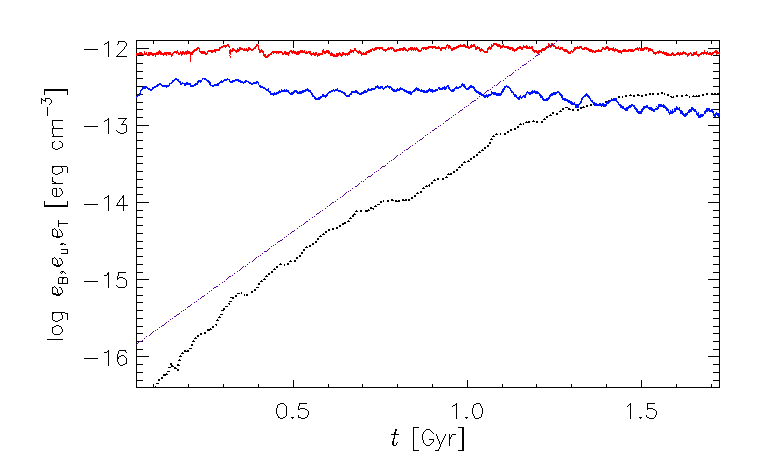
Figure 1: Evolution of energy densities averaged over the whole computational domain; thermal ${\langle e_{\mathrm{T}}\rangle}$ (red), kinetic ${\langle e_{\mathrm{u}}\rangle}$ (blue) and magnetic ${\langle e_{\mathrm{B}}\rangle}$ (black). Guide line (purple, dotted) indicates $\exp(7.5t\,{\rm Gyr}^{-1})$.

Figure 1 demonstrates the nearly exponential growth of magnetic energy density against the (approximately) stationary background of turbulent motions and thermal structure. As the average magnetic energy density ${\langle e_{\mathrm{B}}\rangle}={\langle|{{\mbox{\boldmath$B$}}}|^{2}\rangle}/8\pi$ becomes comparable to the average kinetic energy density ${\langle e_{\mathrm{u}}\rangle}$ at $t>1\,{\rm Gyr}$, the latter shows a modest reduction, as expected for the conversion of the kinetic energy of random motions to magnetic energy. For $t>1.4\,{\rm Gyr}$, magnetic field settles to a statistically steady state ${\langle e_{\mathrm{B}}\rangle}\approx 2.5\times 10^{-13}\,{\rm erg}\,{\rm cm}^{-3}$, somewhat larger than ${\langle e_{\mathrm{u}}\rangle}\approx 1.6\times 10^{-13}\,{\rm erg}\,{\rm cm}^{-3}$, while the thermal energy density ${\langle e_{\mathrm{T}}\rangle}\approx 10^{-12}\,{\rm erg}\,{\rm cm}^{-3}$ appears only weakly affected. Due to changes to the flow and thermodynamic composition, Ohmic heating is offset by reduced viscous heating or more efficient radiative cooling.

Magnetic field $B$ can be decomposed into ${{\mbox{\boldmath$B$}}}_{\ell}$, the part averaged over the length scale $\ell$, and the complementary fluctuations ${{\mbox{\boldmath$b$}}}{\color[rgb]{0,0,0}{{}_{\ell}}}$,

$${{\mbox{\boldmath$B$}}}={{\mbox{\boldmath$B$}}}_{\ell}+{{\mbox{\boldmath$b$}}}{\color[rgb]{0,0,0}{{}_{\ell}}},\quad{{\mbox{\boldmath$B$}}}_{\ell}={\langle{{\mbox{\boldmath$B$}}}\rangle}_{\ell},\quad{{\mbox{\boldmath$b$}}}{\color[rgb]{0,0,0}{{}_{\ell}}}={{\mbox{\boldmath$B$}}}-{{\mbox{\boldmath$B$}}}_{\ell},$$ (2)

using volume averaging with a Gaussian kernel:

$${\langle{{\mbox{\boldmath$B$}}}\rangle}_{\ell}({{\mbox{\boldmath$x$}}}) =\int_{V}{{\mbox{\boldmath$B$}}}({{\mbox{\boldmath$x$}}}^{\prime})G_{\ell}({{\mbox{\boldmath$x$}}}-{{\mbox{\boldmath$x$}}}^{\prime})\,{\rm d}^{3}{{\mbox{\boldmath$x$}}}^{\prime},$$ (3)

$$G_{\ell}({{\mbox{\boldmath$x$}}}) =\left(2\pi\ell^{2}\right)^{-{3}/{2}}\exp\left[-{{{\mbox{\boldmath$x$}}}^{2}}/({2\,\ell^{2}})\right],$$

where $V$ is the volume of the computational domain. This operation preserves the solenoidality of both ${{\mbox{\boldmath$B$}}}_{\ell}$ and ${{\mbox{\boldmath$b$}}}{\color[rgb]{0,0,0}{{}_{\ell}}}$ and retains their three-dimensional structure. For computational efficiency, the averaging was performed in the Fourier space where the convolution of Eq. (3) reduces to the product of Fourier transforms.

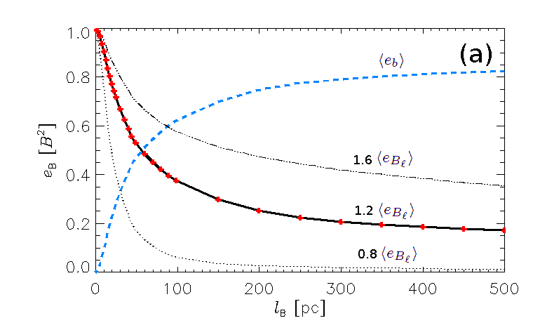
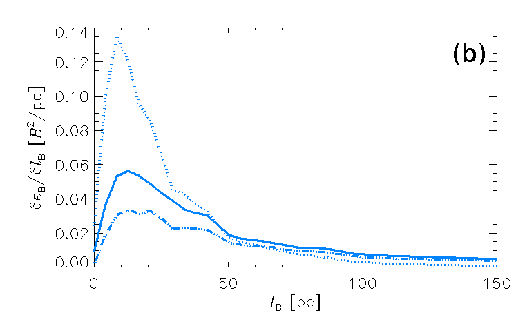
Figure 2: (a) Energy densities at $t=1.2\,{\rm Gyr}$ of mean, ${\langle e_{B_{\ell}}\rangle}$ (black, solid), and fluctuating, ${\langle e_{b}\rangle}$ (blue, dashed), magnetic fields as functions of the averaging length $\ell$, normalized by ${\langle{\langle e_{\mathrm{B}}\rangle}_{\ell}\rangle}$ and averaged over the region $|z|<0.5\,{\rm kpc}$; also ${\langle e_{B_{\ell}}\rangle}$ at $t=0.8\,{\rm Gyr}$ (dotted) and $t=1.6\,{\rm Gyr}$ (dash-triple-dotted). Values of $\ell$ sampled are indicated by red crosses. (b) Derivative of ${\langle e_{b}\rangle}$ from Panel (a) with respect to $\ell$, with the same line types.

Since the averaging (3) does not obey the Reynolds rules for the mean, the definitions of various averaged quantities should be generalized as suggested by Germano (1992). In particular, the local energy density of the fluctuation field is given by

$$e_{b}({{\mbox{\boldmath$x$}}})=\frac{1}{8\pi}\int_{V}|{{\mbox{\boldmath$B$}}}({{\mbox{\boldmath$x$}}}^{\prime})-{{\mbox{\boldmath$B$}}}_{\ell}({{\mbox{\boldmath$x$}}})|^{2}G_{\ell}({{\mbox{\boldmath$x$}}}-{{\mbox{\boldmath$x$}}}^{\prime})\,{\rm d}^{3}{{\mbox{\boldmath$x$}}}^{\prime}.$$ (4)

This ensures that ${\langle e_{B}\rangle}_{\ell}=e_{B_{\ell}}+e_{b}$, where $e_{B}=|{{\mbox{\boldmath$B$}}}|^{2}/(8\pi)$ and $e_{B_{\ell}}=|{{\mbox{\boldmath$B$}}}_{\ell}|^{2}/(8\pi)$. Expanding ${{\mbox{\boldmath$B$}}}({{\mbox{\boldmath$x$}}}^{\prime})$ in a Taylor series around $x$ and using $\int_{V}G_{\ell}({{\mbox{\boldmath$x$}}}-{{\mbox{\boldmath$x$}}}^{\prime})\,{\rm d}^{3}{{\mbox{\boldmath$x$}}}^{\prime}=1$ (normalization) and $\int_{V}({{\mbox{\boldmath$x$}}}-{{\mbox{\boldmath$x$}}}^{\prime})G_{\ell}({{\mbox{\boldmath$x$}}}-{{\mbox{\boldmath$x$}}}^{\prime})\,{\rm d}^{3}{{\mbox{\boldmath$x$}}}^{\prime}=0$ (symmetry of the kernel), it can be shown that $e_{b}=|{{\mbox{\boldmath$b$}}}{\color[rgb]{0,0,0}{{}_{\ell}}}|^{2}/(8\pi)+O(\ell/L)^{2}$, where $L$ is the scale of the averaged magnetic field defined as $L^{2}=|{{\mbox{\boldmath$B$}}}_{\ell}|/|\nabla^{2}{{\mbox{\boldmath$B$}}}_{\ell}|$ in terms of the characteristic magnitude of ${{\mbox{\boldmath$B$}}}_{\ell}$ and its second derivatives. Thus the difference between the ensemble and volume averages rapidly decreases as the averaging length increases, $\ell/L\to 0$, or if the averaging is performed over the whole space, $L\to\infty$; this quantifies the deviations from the Reynolds rules for finite $\ell/L$.

The appropriate choice of $\ell$ is not obvious. We consider a range $0<\ell<500\,{\rm pc}$, applying the averaging to 37 snapshots of the magnetic field between $t=0.8$ and 1.7 Gyr; the results for $t=0.8$, 1.2 and $1.6\,{\rm Gyr}$ are shown in Fig. 2. The smaller is $\ell$, the closer the correspondence between the averaged field and the original field (since the average is effectively sampling a smaller local volume), and hence the smaller the part of the total field considered as the fluctuation. Hence ${\langle B_{\ell}^{2}\rangle}$ is a monotonically decreasing function of $\ell$, whereas ${\langle b{\color[rgb]{0,0,0}{{}_{\ell}}}^{2}\rangle}$ monotonically increases (Fig. 2a). Our aim is to identify that value of $\ell$ where the variation of ${{\mbox{\boldmath$B$}}}_{\ell}$ and ${{\mbox{\boldmath$b$}}}{\color[rgb]{0,0,0}{{}_{\ell}}}$ with $\ell$ becomes weak enough. To facilitate this, we consider the rate of change of the relevant quantities with $\ell$, shown in Fig. 2b (note the different scale of the horizontal axis in this panel). The length $\ell\approx 50\,{\rm pc}$ is clearly distinguished: all the curves in Panel (b) are rather featureless for $\ell>50\,{\rm pc}$. The values in Fig. 2 have been obtained from the part of the domain with $|z|<0.5\,{\rm kpc}$, where most of the gas resides and where dynamo action is expected to be most intense. The results, however, remain quite similar if the whole computational domain $|z|\leq 1\,{\rm kpc}$ is used. While this value of $\ell$ has been estimated in a rather heuristic and approximate manner, the analysis of the magnetic power spectra in Section 4 confirms that $\ell=50\,{\rm pc}$ is close to the optimal choice.

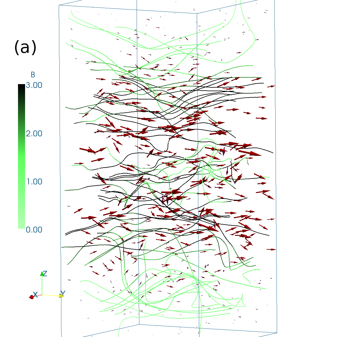
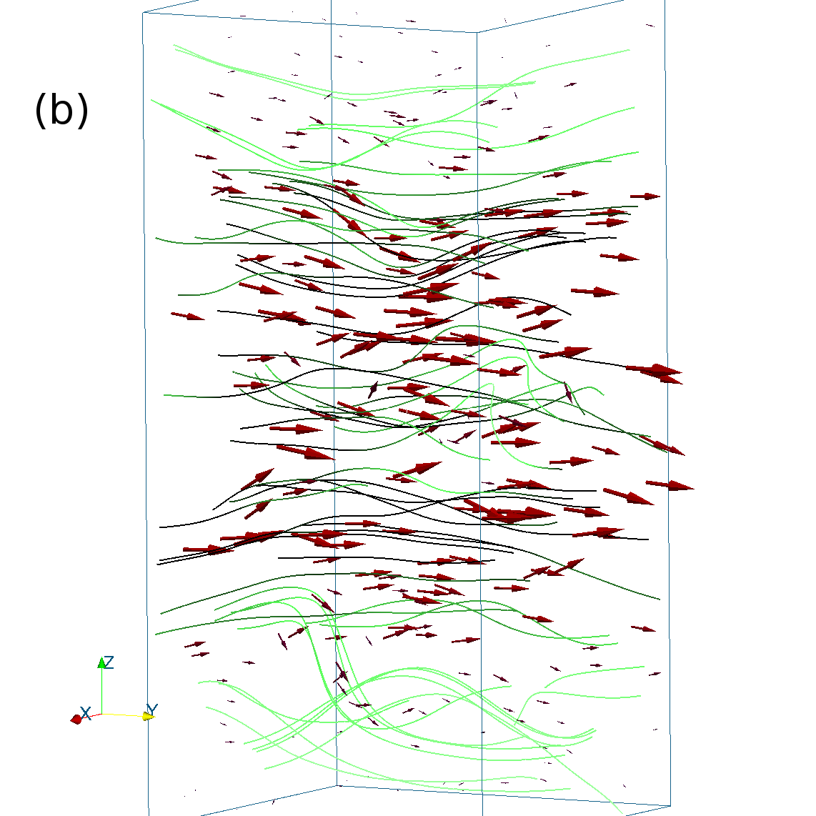
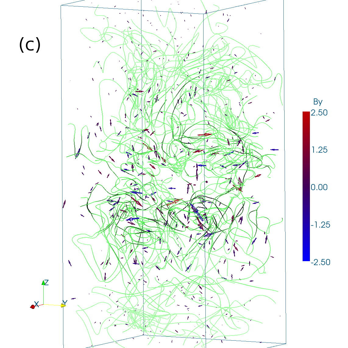
Figure 3: Field lines of (a) the total magnetic field $B$, (b) its averaged part ${{\mbox{\boldmath$B$}}}_{\ell}$, (c) the fluctuations ${{\mbox{\boldmath$b$}}}{\color[rgb]{0,0,0}{{}_{\ell}}}$, obtained by averaging with $\ell=50\,{\rm pc}$, for $t=1.625\,{\rm Gyr}$. Field directions are indicated by arrows. The colour of the field lines indicates the field strength (colour bar on the left), whereas the vectors are coloured according to the strength of the azimuthal ($y$) component (colour bar on the right).

To put the estimate $\ell\approx 50\,{\rm pc}$ into context, we note that it is about half the integral scale of the random motions, $l_{0}$, in a similar model of Paper I. Simulations of a single SN remnant in an ambient density similar to that at $z=0$, reported in Paper I, also show that the expansion speed of the remnant reduces to the ambient speed of sound when its radius is 50–70 pc.

Figure 3 illustrates the total, mean and random magnetic fields thus obtained. For this saturated state, the field has a very strong uniform azimuthal component and a weaker radial component. The orientation of the field is the same above and below the mid-plane ($B_{y}>0$ and $B_{x}<0$), with maxima located at $|z|\approx 0.2\,{\rm kpc}$; the results will be reported in detail elsewhere.

4 Scale separation

Scale separation between the mean and random magnetic fields in natural and simulated turbulent dynamos can be difficult to identify. The signature of scale separation sought for is a pronounced minimum in the magnetic power spectrum at an intermediate scale, larger than the energy-range scale of the random flow and smaller than the size of the computational domain. The power spectrum for $B$ is ${\color[rgb]{0,0,0}{M(k)=k^{-2}{{\langle|\mathcal{F}({k})|\rangle}_{k}},}}$ for spherical shells of thickness $\delta k$ at radius $k=|{{\mbox{\boldmath$k$}}}|$, from ${\color[rgb]{0,0,0}{\mathcal{F}({{\mbox{\boldmath$k$}}})={\int_{V}{{\mbox{\boldmath$B$}}}({{\mbox{\boldmath$x$}}})\exp({-2\pi i{{\mbox{\boldmath$k$}}}\cdot{{\mbox{\boldmath$x$}}}}){\rm d}^{3}{{\mbox{\boldmath$x$}}}}.}}$ The spectra of the mean and random magnetic fields obtained by Gaussian smoothing, shown in Fig. 4, have maxima at significantly different wavenumbers. We note that the spectrum of the total magnetic field does not have any noticeable local minima and, with the standard approach (e.g., based on horizontal averages), the system would be considered to lack scale separation.

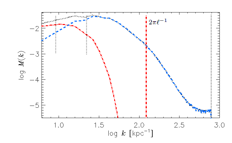
Figure 4: Power spectra of total (black, dotted), mean (red, dash-dotted) and fluctuating (blue, dashed) magnetic fields, for Gaussian smoothing with $\ell=50\,{\rm pc}$, at $t=1.05\,{\rm Gyr}$. Vertical red (dash-dotted) line marks the averaging wavenumber $2\pi\ell^{-1}$ and vertical black (dotted) line indicates the Nyquist wave number $\pi\Delta^{-1}$. Short vertical segments mark the energy-range scales $2\pi{L}_{\ell}^{-1}$ and $2\pi{L}_{b}^{-1}$ of the mean and random magnetic fields, respectively, obtained from Eq. (5).

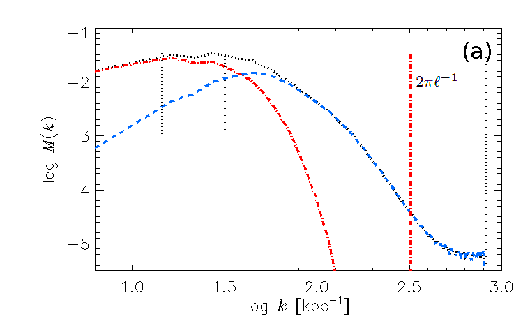
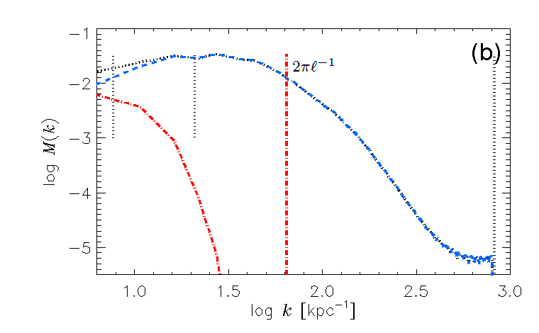
Figure 5: As Fig. 4, but for (a) $\ell=20\,{\rm pc}$ and (b) $\ell=100\,{\rm pc}$.

Figure 4 shows the magnetic power spectra of $B$, ${{\mbox{\boldmath$B$}}}_{\ell}$ and ${{\mbox{\boldmath$b$}}}{\color[rgb]{0,0,0}{{}_{\ell}}}$. Note that $\ell$ is not located between the maxima in the power spectra of ${{\mbox{\boldmath$B$}}}_{\ell}$ and ${{\mbox{\boldmath$b$}}}{\color[rgb]{0,0,0}{{}_{\ell}}}$; in fact, the spectral density of the mean field is negligible for $k\simeq 2\pi\ell^{-1}$. This can be understood from the transform of the kernel $G_{\ell}({{\mbox{\boldmath$x$}}})$, i.e. $\widehat{G}_{\ell}({{\mbox{\boldmath$k$}}})=\exp(-\ell^{2}{{\mbox{\boldmath$k$}}}^{2}/2)$; this kernel would divide a purely sinusoidal field equally into the mean and random parts at the wavelength $\lambda_{\rm eq}=\sqrt{2/\ln 2}\,~{}\pi\ell$. For $\ell=50\,{\rm pc}$, $\lambda_{\rm eq}=0.27\,{\rm kpc}$, and the latter figure is a better guide to the expected separation scale. The separation of scales is immediately apparent in the spectra of the mean and random fields, $M_{\ell}(k)$ and $M_{b}(k)$, with the former having a broad absolute maximum at about $0.56\,{\rm kpc}$ and the latter, a broad maximum near $0.2\,{\rm kpc}$. The effective separation scale $\lambda{\color[rgb]{0,0,0}{{}_{\rm eq}}}\approx 0.48\,{\rm kpc}$ can be identified where $M_{\ell}(k)=M_{b}(k)$, i.e. where the curves cross at $\log k\simeq 1.1$. $\lambda>\lambda_{\rm eq}$ mainly characterize the mean and $\lambda<\lambda_{\rm eq}$ the random field.

The integral scales of ${{\mbox{\boldmath$B$}}}_{\ell}$ and ${{\mbox{\boldmath$b$}}}{\color[rgb]{0,0,0}{{}_{\ell}}}$ can be obtained from their spectral densities as

$${L}_{\ell}=\frac{\pi}{2}\,{\int_{{2\pi}/{D}}^{{\pi}/{\Delta}}k^{-1}M(k)\,{\rm d}k}\left[{\int_{{2\pi}/{D}}^{{\pi}/{\Delta}}M(k)\,{\rm d}k}\right]^{-1},$$ (5)

where $\Delta$ is the numerical grid separation and $D$ is the size of the domain (Section 12.1 Monin & Yaglom, 2007). This yields ${L}_{\ell}\simeq 0.67\,{\rm kpc}$ and ${L}_{b}\simeq 0.28\,{\rm kpc}$ for ${{\mbox{\boldmath$B$}}}_{\ell}$ and ${{\mbox{\boldmath$b$}}}{\color[rgb]{0,0,0}{{}_{\ell}}}$, respectively (Fig. 4).

As the magnetic field strength grows, the magnitudes of the spectral densities change but the characteristic wavenumbers vary rather weakly. ${L}_{\ell}$ remains close to $0.7\,{\rm kpc}$ throughout the kinematic phase, increasing only beyond 1.1 Gyr to about $0.9\,{\rm kpc}$. ${L}_{b}$ increases from $0.23$ to $0.28\,{\rm kpc}$ during the kinematic phase, but rises to $0.4\,{\rm kpc}$ after the system saturates. The stability of ${L}_{\ell}$ is consistent with the eigenmode amplification of the mean magnetic field as expected for a kinematic dynamo, and supports $\ell\approx 50\,{\rm pc}$ as a reasonable choice of the averaging scale.

Figure 5 presents magnetic energy spectra obtained using $\ell=20\,{\rm pc}$ and $100\,{\rm pc}$. In the former, the effective separation scale $\lambda{\color[rgb]{0,0,0}{{}_{\rm eq}}}\approx 0.16\,{\rm kpc}$ is less than ${L}_{b}\simeq 0.21\,{\rm kpc}$. This is inconsistent, implying that energy at scales about ${L}_{b}$ lies predominantly within ${{\mbox{\boldmath$B$}}}_{\ell}$. For $\ell=100\,{\rm pc}$, $\lambda{\color[rgb]{0,0,0}{{}_{\rm eq}}}\geq 1\,{\rm kpc}$ is greater than ${L}_{\ell}\simeq 0.81\,{\rm kpc}$, which is also inconsistent. Significantly, applying $\ell=50\,{\rm pc}$ satisfies ${L}_{b}<\lambda<{L}_{\ell}$. Hence the scale $\lambda$, at which the dominant energy contribution switches between the mean and fluctuating parts, is here consistent only with $\ell\simeq 50\,{\rm pc}$.

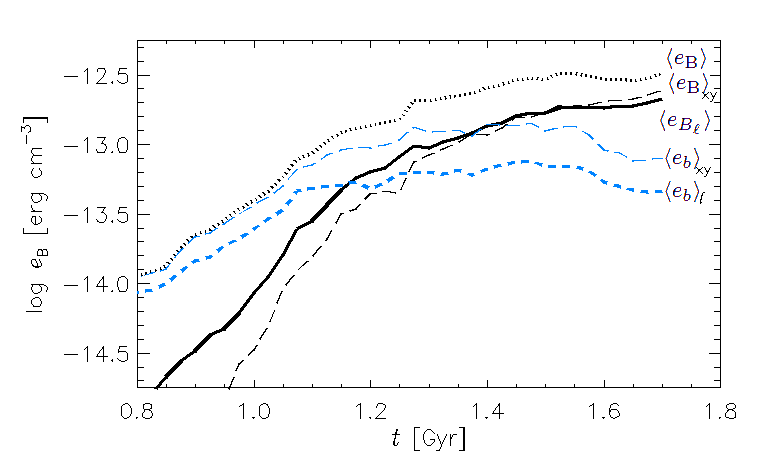
Figure 6: Evolution of magnetic energy densities, averaged for full domain: total magnetic field (black, dotted), mean (black, solid), and random (blue, dashed) obtained from Gaussian smoothing with $\ell=50\,{\rm pc}$. Energy densities of mean and random magnetic fields obtained from horizontal averaging are shown long-dashed (black and blue, respectively).

As well as different spatial scales, the mean and random magnetic field energies have different exponential growth rates (Fig. 6), given in Table 1. Results from horizontal averaging are also given; they differ from those obtained with Gaussian smoothing, especially for the mean field. The growth rate $\Gamma$ of the mean-field energy is controlled by the shear rate, mean helicity of the random flow, and the turbulent magnetic diffusivity. Any mean magnetic field is accompanied by a random field, which is part of the mean-field dynamo mechanism (as any large-scale magnetic field is tangled by the random flow); the energy of this part of the small-scale field should grow at the same rate $\Gamma$ as the mean energy. The fluctuation dynamo produces another part of the random field whose energy growth rate depends on the turbulent kinematic time scale $l/u$, and the magnetic Reynolds and Mach numbers. The difference between $\Gamma$ and $\gamma$ obtained suggests that both mean-field and fluctuation dynamos are present in our model. The growth rate of the mean magnetic energy is roughly double that of the random field for both types of averaging. This is opposite to what is usually expected, plausibly because of the inhibition of the fluctuation dynamo by the strongly compressible nature of the flow, and by the low Reynolds numbers available at this resolution. We would expect the fluctuation dynamo to be stronger with more realistic Reynolds numbers.

Table 1: Exponential growth rates of energy in the mean and random magnetic fields, $\Gamma$ and $\gamma$, respectively, with associated values of reduced $\chi^{2}$. From exponential fits to the corresponding curves in Fig. 6, for $0.8<t<1.05\,{\rm Gyr}$. (Growth for $t<0.8\,{\rm Gyr}$ is similar to this interval – see Fig. 1.)

	$\Gamma$	$\chi^{2}$	$\gamma$	$\chi^{2}$
	[Gyr-1]		[Gyr-1]
Gaussian smoothing	$10.9$	$1.00$	5.5	$1.15$
Horizontal averaging	$13.6$	$0.25$	$6.2$	$0.25$

5 Discussion

The approach used here to identify the appropriate averaging length $\ell$ (and thus the effective separation scale $\lambda$) is simple (but not oversimplified); $\ell$ can in fact depend on position, and it can remain constant in time only at the kinematic stage of all the dynamo effects involved. Wavelet filtering may prove to be more efficient than Gaussian smoothing in assessing the variations of $\ell$.

At the kinematic stage, the spectral maximum of the mean field is already close to the size of the computational domain, and it cannot be excluded that the latter is too small to accommodate the most rapidly growing dynamo mode. These results should therefore be considered as preliminary with respect to the mean field; simulations in a bigger domain are clearly needed.

The physically motivated averaging procedure used here, producing a mean field with three-dimensional structure, may facilitate fruitful comparison of numerical simulations with theory and observations. Although Gaussian smoothing does not obey all the Reynolds rules, it is possible that a consistent mean-field theory can be developed, e.g. in the framework of the $\tau$-approximation (see e.g. Brandenburg & Subramanian, 2005, and references therein). This approach does not rely upon solving the equations for the fluctuating fields, and hence only requires the linearity of the average and its commutation with the derivatives. The properly isolated mean field is likely to exhibit different spatial and temporal behaviour than the lower-dimensional magnetic field obtained by two-dimensional averaging.

References

- Beck et al. (1996) Beck R., Brandenburg A., Moss D., Shukurov A., Sokoloff D., 1996, ARA&A, 34, 155
- Brandenburg & Subramanian (2005) Brandenburg A., Subramanian K., 2005, Phys. Rep., 417, 1
- Eyink (2005) Eyink G. L., 2005, Physica D, 207, 91
- Eyink (2012) Eyink G. L., 2012, Turbulence Theory (Course Notes), John Hopkins Univ., http://www.ams.jhu.edu/eyink/Turbulence/
- Gent et al. (2012) Gent F. A., Shukurov A., Fletcher A., Sarson G. R., Mantere M. J., 2012, MNRAS (Paper I)
- Germano (1992) Germano M., 1992, J. Fluid Mech., 238, 325
- Gressel et al. (2008) Gressel O., Elstner D., Ziegler U., Rüdiger G., 2008, A&A, 486, L35
- Monin & Yaglom (2007) Monin A. S., Yaglom A. M., 2007, Statistical Fluid Mechanics, Vol. I, Dover
- Shukurov (2007) Shukurov A., 2007, in Dormy E., Soward A. M., eds, Mathematical Aspects of Natural Dynamos, Chapman & Hall/CRC, pp 313–359
- Sokoloff et al. (1983) Sokoloff D., Shukurov A., Ruzmaikin A., 1983, Geophys. Astrophys. Fluid Dyn., 25, 293
- Starchenko & Shukurov (1989) Starchenko S. V., Shukurov A. M., 1989, A&A, 214, 47