Evaluating the dependence of a non-leaky intervention’s partial efficacy on a categorical mark

Abstract

We address discrete-marks survival analysis, also known as categorical sieve analysis, for a setting of a randomized placebo-controlled treatment intervention to prevent infection by a pathogen to which multiple exposures are possible, with a finite number of types of “failure”. In particular, we address the case of interventions that are partially efficacious due to a combination of failure-type-dependent efficacy and subject-dependent efficacy, for an intervention that is “non-leaky” (where “leaky” interventions are those for which each exposure event has a chance of resulting in a “failure” outcome, so multiple exposures to pathogens of a single type increase the chance of failure). We introduce the notion of some-or-none interventions, which are completely effective only against some of the failure types, and are completely ineffective against the others. Under conditions of no intervention-induced failures, we introduce a framework and Bayesian and frequentist methods to detect and quantify the extent to which an intervention’s partial efficacy is attributable to uneven efficacy across the failure types rather than to incomplete “take” of the intervention. These new methods provide more power than existing methods to detect sieve effects when the conditions hold. We demonstrate the new framework and methods with simulation results and new analyses of genomic signatures of HIV-1 vaccine effects in the STEP and RV144 vaccine efficacy trials.

1 Introduction

Despite advances in both treatment and prevention, the global HIV/AIDS epidemic continues to levy a heavy toll on millions of HIV-infected individuals and those who love them. With a global prevalence of over 33 million, and an estimated 14% prevalence among women and men aged 15-49 in some subsaharan African states where non-vaccine interventions are difficult to scale to a population level, there is great need for an effective public health vaccine (HIVPrevalence).

There is no licensed vaccine to prevent infection by HIV. While some vaccines have been relatively easy to develop, creating effective vaccines against HIV has proven more challenging. In response to the slow pace of the traditional strategy for vaccine development, organizations such as the Global HIV-1 Vaccine Enterprise are advocating for more iterative strategies, in which even “failed” clinical trials nevertheless provide maximal insight into mechanisms of whatever partial protection may have been conferred to some subset of vaccine recipients (GlobalVaccineEnterprise2010).

One critical question that arises in such an approach is, in the aftermath of a randomized clinical trial to evaluate a new treatment intervention, to what extent should observed differences in apparent efficacy across outcome types be attributed to actual imbalanced efficacy across those types, as opposed to imbalanced uptake across subjects, or to just poor efficacy overall? This is non-trivial because other factors may also lead to a difference in observed failure rates across types, other than differential efficacy of the intervention to prevent type-specific failures.

A sieve analysis investigates an interventions’s efficacy as a function of specific features of the outcome (edlefsen2013current). A recent example comes from a sieve analysis of the RV144 HIV-1 vaccine efficacy trial. The RV144 vaccine regimen was partially efficacious at reducing HIV-1 acquisition risk among healthy low-risk Thai volunteers, with an estimated intervention efficacy (IE) of 31% versus placebo (Ngarm). A subsequent sieve analysis identified that this efficacy significantly differed against viruses of two types that are differentiated by a viral genome feature at an immunologically relevant locus (v2sieve). This result concords with other evidence that the vaccine induced antibodies that target a specific region (called V2) of the viral envelope (haynes2012immune), and together these results are influencing ongoing and planned HIV-1 vaccine trials.

Sieve analysis can also provide valuable insight into an intervention’s effect in the context of an intervention with no overall efficacy. An example comes from the STEP HIV-1 vaccine efficacy trial, which was halted early for efficacy futility (Buchbinder). STEP evaluated a vaccine candidate in high-risk study participants in the Americas. At its early conclusion, the estimated hazard ratio of infection (vaccine vs placebo) was about 1.5. A sieve identified vaccine-driven selective pressure at an immunologically-relevant HIV-1 locus, indicating that although it did not reduce the overall acquisition rate, the vaccine did induce an immune response that affected the distribution of observed viruses, possibly by altering the dynamics of post-infection viral evolution (Rolland).

Sieve analysis is also known as “mark-specific efficacy analysis”, where the general term “mark” refers to features of the failure (as opposed to covariates of the subject). Sieve analysis methods have been developed for a variety of types of marks (e.g. GSA; GMS; juraska2013mark). Common example features include pathogen serotypes, and quantitative measures of pathogen susceptibility to neutralization. The framework that we introduce in this article addresses finite-category nominal marks.

Peter Gilbert enumerated several conditions that are required to yield unbiased estimates of mark-specific intervention efficacy for the case of a “leaky” intervention (GSA; gilbert2001interpretability). The notion of a “leaky” intervention was introduced by struchiner1990behaviour in contrast with an “all-or-none” intervention (halloran1991direct) for a setting in which failure types are not differentiated, and has been extensively developed for applications in that setting (halloran2010design). In the former case, each of a subject’s potentially-multiple exposures has some chance of being thwarted by the effect of the intervention; in the latter case, each subject is either a responder (and therefore protected if exposed) or not. In vaccine trials, responders are said to have “take” of the vaccine.

Peter Gilbert argued and showed through simulation studies that his conditions for unbiased sieve analysis are violated whenever some subjects have no “take” (gilbert2000comparison). We introduce a new variant on the “leaky” vs “all-or-none” dichotomy: the “sievey-not-leaky” intervention, which exhibits sieve effects but not per-event stochastic leaks. We call such an intervention “some-or-none”, as it completely protects subjects with “take” - but only against failures with marks that fall in an “intervention-targeted” subset. We provide analogous conditions for unbiased assessment of sieve effects in this non-leaky setting, and introduce the “sievey-not-leaky” modeling framework for evaluating a some-or-none intervention under the “no-harm” condition (that the intervention can prevent would-be-failures but cannot induce new failures or increase susceptibility).

We also provide a new perspective on the “Model-Based Sieve” (MBS) method that was employed in the RV144 sieve analysis (v2sieve), and show that it can be understood either as an approximation to the some-or-none intervention model or as a model of the effects of the intervention on post-infection variation.

The scope of the present work is limited to categorical representations of all outcomes. Future work incorporating time-to-event data into the framework is likely to improve efficiency of the methods. Note too that this representation necessitates excluding subjects lost-to-followup before the end of the trial (assuming conditions of uninformative missingness), who may contribute information relevant to estimation of intervention efficacy but would not (in this framework) contribute to the estimation of relative failure rates across failure types.

In the Results section we present new analyses of the genomic sequences of the HIV-1 viruses that infected participants of the RV144 and STEP trials, in which the mark types are the amino acids (AAs) found in the genome of each virus at a particular locus of interest. In that setting, one particular AA is unique because it was included in the vaccine (so we expect that sieve effects will reflect greatest efficacy against this targeted category) but the other AAs are unordered. We address the general problem of sieve analysis for unordered categories, and are particularly motivated by settings in which some categories are targets of the intervention and others are not.

The remainder of this article is organized as follows. First we describe the “sievey-not-leaky” (SNL) modeling framework. Although we assume that the intervention does not induce new failures, sieve effects may lead to type-specific increases in the observed failure rates due to replacement of avoided failures by failures of other types. We discuss the potentially confounding effects of such “replacement causes” on efforts to detect sieve effects, and describe conditions under which observed changes to failure type distributions are attributable to sievey-not-leaky sieve effects. We outline methods to test these conditions and present Bayesian and frequentist methods to detect sieve effects when the conditions hold. To our knowledge, this is the first application of Bayesian methodology to the problem of sieve analysis.

2 Sievey-not-leaky modeling of intervention efficacy

2.1 Notation

As we introduce the SNL framework and some-or-none models, we will use the following notational conventions. All vector-valued parameters are in bold and parameter vectors are named consistently so that their dimensionality and role is apparent. Lowercase subscripts convey either the main role of the parameter, the treatment group to which it corresponds, or an index into the (vector-valued) parameter. Table 1 describes the relevant symbols.

Table 1: Notation symbols and their meanings

				role	index
category	symbol	meaning	range	subscripts	subscripts
	$J$	number failure categories	$\mathcal{N}^{+}$
	$g$	number targeted categories	$1\dotsc J$
	$R$	set of response categories	$R=\{0,1\}$
	$\tau$	(time) duration of the trial	$\mathcal{R}^{+}$
initial	$z$	treatment group	$\{\hbox{p},\hbox{v}\}$		$i$
initial	$n$	outcome count	$\mathcal{N}$	$p$, $v$, $c$	$j$
initial	$p$	probability	$[0,1]$	$r$, $s$
initial	$r$	“take” response indicator	$R$		$i$
initial	$\bm{Y}$	outcomes for each subject	$0\dotsc J$	$p$, $v$, $c$	$i$
initial	$\bm{n}$	count simplex	$[0,1]^{J+1}$	$p$, $v$, $c$	$j$
initial	$\bm{r}$	probability simplex	$[0,1]^{J+1}$	$p$, $v$, $c$	$j\geq 0$
initial	$\bm{p}$	probability simplex	$[0,1]^{J}$	$p$, $v$, $c$	$j>0$
initial	$\bm{q}$	probability simplex	$[0,1]^{J-g}$	$p$, $v$, $c$	$j>g$
initial	$\bm{t_{i}}$	exposure times for subject $i$	$(0,\tau)$		$j>0$
initial	$\bm{\omega_{r}}$	failure avoidance rates for response $r$	$[0,1]$		$j>0$
subscript	$i$	index for subjects	$1\dotsc n$
subscript	$j$	index for outcome types	$0\dotsc J$
subscript	$p$	control treatment group
subscript	$v$	intervention treatment group
subscript	$c$	counterfactual for intervention group
special	$t$	$p_{t}\equiv Pr(\hbox{``take'' response})$
special	$2$	$p_{2}\equiv Pr(\hbox{avoided failure is replaced})$
special	$s$	$p_{s}\equiv$ the “sieve effect strength”

We begin with (categorical, completely observed) outcome data $\bm{Y}$ for all $n=n_{v}+n_{p}$ subjects of a (placebo-)controlled randomized trial, with $\bm{Y_{v}}$ denoting the outcomes for just the $n_{v}$ intervention recipients (that is, for those subjects for whom $z_{i}=v$). Outcome types $j$ include the special value $0$ to indicate non-failure, and the other (failure) types are labeled such that $1$ through $g$ are failure types that are targeted by the $g$-or-none intervention. For instance $n_{p0}$ of the $n_{p}\equiv\sum_{j=0}^{J}n_{pj}$ control recipients had not failed by the end of the trial, and $n_{v1}$ of the $n_{v}\equiv\sum_{j=0}^{J}n_{vj}$ treatment intervention recipients failed with failure type $1$.

We let “c” (as a subscript) represent the counterfactual values of what would be seen in the treatment group if they had not received the treatment. So for instance we define the counterfactual total number of subjects $n_{c}$ as $\sum_{j=0}^{J}n_{cj}$, which is equivalent to $n_{v}$ since by assumption the intervention does not affect the total number of subjects (just which subjects fail, and their corresponding failure types).

Uppercase subscripts (“G”) in the index position indicate a scalar sum over indices $1\dotsc g$. For example, $r_{cG}=\sum_{j=0}^{g}{p_{cj}}$ is the probability that a treatment-intervention recipient would have a targeted-type failure if that subject had not received the intervention. Parameters with initial “r” refer to outcome proportions, with “p” refer to failure proportions, and with “q” refer to non-targeted-type proportions; so for example $r_{pJ}\equiv\frac{n_{pJ}}{n_{p}}$, vs $p_{pJ}\equiv\frac{n_{pJ}}{n_{p}-n_{p0}}$, vs $q_{pJ}\equiv\frac{n_{pJ}}{n_{p}-(n_{p0}+n_{pG})}$. Note that we also use $\bm{q}$ without a treatment group subscript to indicate the distribution among non-targeted categories of replacement failures, as discussed below.

To be consistent with the literature on discrete marks sieve analysis, we parameterize our approach to comparing some-or-none to all-or-none models in terms of the failure type frequencies $p_{vj}$ and $p_{pj}$. Although when optimizing parameters (for maximum-likelihood estimation) we may employ the logistic transform for more convenient search, in this article we represent the category probabilities directly in their own simplex scale (rather than the logistic scale). As all of the model parameters index either a binomial or multinomial distribution family, when being Bayesian we use conjugate beta or Dirichlet priors on this simplex scale.

2.2 No-harm, would-be-first failure processes, and replacement failures

In accord with the definition used in GSA, we define mark-specific intervention efficacy in terms of “per-exposure” probabilities of infection (failure), given one exposure event. Since we are not able to observe exposures, and since a single subject may experience zero or multiple exposure events, we are not generally able to directly estimate these per-exposure probabilities (rhodes1996counting). GSA showed that under certain (leaky) conditions, relative risks and odds ratios of these probabilities are directly estimable.

Departing somewhat from these and other articles’ definitions of “exposure”, in this article (and in the framework here introduced) we simplify the setting to assume that “exposure” is defined as “an exposure that would, in the absence of intervention, result in a failure”. Thus the per-exposure probability of failure is $1$ for placebo recipients (and for intervention recipients in the counterfactual case) for any type of failure, and variations of failure rates across types for these subjects are due solely to variations in exposure distributions across the failure types. Note that this definition precludes the possibility that an intervention-receiving subject would experience a new failure that would not be experienced in the counterfactual case. This is the “no-harm” assumption.

However, since an intervention-receiving subject might avoid (due to the intervention) the failure that would have affected him in the counterfactual case, and is thus potentially susceptible to subsequent exposures, there may be “replacement failures” affecting intervention recipients that would never have been observed in the counterfactual case (since a subject’s observed failure is defined as her first exposure that is not avoided).

When there are $J$ failure types, this exposure model is equivalent to a $J$ competing risks model in which only the time of the “winning” exposure process is observed, where “winning” additionally requires that the exposure is not avoided due to the intervention. Concretely, we represent the $J$ competing risks for each subject $i$ with $J$ simultaneous (and possibly jointly-distributed) continuous-time Markov counting processes $N_{ij}(t)$, $j\in 1,\dotsc,J$, where at time $t$ the state of process $N_{ij}(t)$ is a natural number indicating the number of potential failure events of type $j$ that subject $i$ would experience by time $t$ if all such potential failures up to time $t$ were avoided (that is, they did not become actual failures) due to the intervention.

This is subtle, but it is important to note that $N_{ij}(t)$ is not the same as the counting process of subject $i$’s actual failures, $N^{\prime}_{ij}(t)$, in which the probability of a subsequent actual failure, given all previous failures, reflects a potential change in the subject’s susceptibility due to the previous failures. Instead, process $N_{ij}(t)$ always reflects the surviving subject’s chance of experiencing an exposure, and the state of this process represents the number of previous would-be-failures that were avoided due to the intervention effect.

This formulation assumes independence between the failure processes of every pair of subjects. Note, though, that we assume nothing particular about the failure processes $N_{ij}(\cdot)$ for any one subject $i$: they may be arbitrarily jointly distributed across the $J$ types. In particular we do not assume that they are memoryless or of any exponential family.

By construction, a subject who does not receive the intervention will never experience an intervention-induced failure avoidance. We nevertheless define these “would-be-first failure processes” for all subjects; any control-recipient subject for whom any of the $J$ processes $N_{ij}(\tau)$ is non-zero at the end of the trial will have $Y_{i}>0$ (since any subject $i$ with $z_{i}=p$ will experience a failure of type $j$ by time $\tau$ whenever $N_{ij}(\tau)>0$). Since the failure type is defined as the mark of the first failure that actually occurs during the trial, we can define control-recipient failure types in terms of the would-be-first failure processes as $Y_{i}=\operatornamewithlimits{argmin}\limits_{j}t_{ij}$, where $t_{ij}\equiv\operatornamewithlimits{argmin}\limits_{t}{N_{ij}(t)I\left(N_{ij}(t)>0\right)}$, or $Y_{i}=0$ if all $J$ times $t_{ij}$ are greater than $\tau$.

2.3 Response types $R$

There may be a subgroup of treatment intervention recipients for whom the treatment did not have any relevant effect. In general we allow for a subject-specific latent (unmeasured) response variable $r_{i}\in R$ to represent subject $i$’s response to the intervention (eg. immune response to vaccination), with the constraint that a unique value in the set $R$ represents “no response” ($r_{i}=0$), and that all control recipients (subjects for whom $z_{i}=p$) have $r_{i}=0$. We let $p_{t}$ represent the rate of non-zero responses among intervention recipients (understood as an expected value over possibly varying subject-specific response rates $p_{ti}$, so $p_{t}\equiv E_{i}[Pr(r_{i}\neq 0|z_{i}=v)]$).

For simplicity of presentation we here consider only binary responses, $R\equiv\{0,1\}$, where subjects for whom $r_{i}=1$ are the subjects with “take”, whose failures are potentially influenced by the intervention. We henceforth use the terms “responders” and those with “take” interchangeably. In a setting such as genome-scan sieve analysis, in which multiple features (genomic loci) are evaluated, the definition of “take” might be feature-specific, as in, “the subject experienced vaccine-induced immune responses that target this locus.” We do not represent “take” on a per-failure-type basis. In the Discussion section (below) we address the extension of this “dichotomous-take” framework to a setting with multiple response types, which includes the special case of models with independent per-failure-type response rates.

2.4 Failure avoidance rate vectors $\{\bm{\omega_{r}}:r\in R\}$, some-or-none interventions

For any particular response type $r\in R$ let there be a vector $\bm{\omega_{r}}$ of $J$ values, with the value at index $j$ (denoted $\omega_{rj}$) representing the per-event (aka “per-exposure”) probability that a subject with treatment response $r$ avoids an event that would, in the absence of the intervention, have caused a failure of type $j$. We assume that these avoidance rates are constant in time, leaving to future work the interesting extension to time-varying efficacy.

The setting of multiple failure types leads to an interesting variation on the “all-or-none” versus “leaky” treatment intervention dichotomy. By definition, treatment interventions exhibiting sieve effects can never be “all-or-none” (which would have equal and perfect avoidance for all takers regardless of failure type); but they could be “some-or-none” (or “one-or-none”) if for all $r$ and $j$, $\omega_{rj}\in\{0,1\}$ but there exists some pair of types $(j,j^{\prime})$ for which $\omega_{rj}\neq\omega_{rj^{\prime}}$. Such an intervention induces (in takers) perfect avoidance of some but not all failure types (at any particular time). Consider, for concreteness, a dichotomous-take one-or-none intervention with $\bm{\omega_{1}}=(1,0,\dots,0)$. We do not consider this a “leaky” intervention, since all of the IE is determined through the take indicator $r_{i}$, with no per-event stochastic filtering.

When it is not known a priori which type(s) might be the targets of the intervention, the one-or-none and some-or-none models can be used in concert to compare different hypotheses regarding the nature of a particular sieve effect. When the SNL sieve conditions hold (see below), and particularly under the condition that the intervention is non-leaky, these models reflect all possible sieve effects for which avoidance rates that are non-zero are the same for all types at any given time. In a Bayesian setting, for instance, we can compute the posterior probability of every possible some-or-none SNL model and compare these to the posterior probability of the all-or-none null model.

We can also compare particular pairs of models using their posterior probabilities, or by using likelihood ratio tests or Bayes factors. For instance we can compare the all-or-none sieve null model (in which treatment recipient relative failure type rates are the same as the counterfactual distribution, which we estimate from the control-recipient data) to the particular one-or-none model in which takers avoid all type-$1$ failures. In the absence of replacement failures, the only effect of the one-or-none intervention is to reduce the type-$1$ failure rate for “takers” by $p_{t}$, so this test compares a model reducing just type-$1$ rates by $p_{t}$ to a model reducing all rates by $p_{t}$.

2.5 The cause replacement rate $p_{2}$

We can make the notion of replacement failures precise in the specific context of some-or-none interventions with target types $1,\dotsc,g$ ($\omega_{1j}=I(1\leq j\leq g)$). In this context, replacement causes imply that $(n_{v0}+n_{vG})<(n_{c0}+n_{cG})$. Put another way, replacement failures cause some treated subjects to fail with a non-targeted failure type who would (in the absence of treatment) have failed with a targeted failure type, so $\sum_{j=(g+1)}^{J}n_{vj}>\sum_{j=(g+1)}^{J}n_{cj}$.

If we assume that a dichotomous-take some-or-none intervention is completely effective (for subjects with relevant responses) at preventing failures of types $1$ through $g$, then the expected number of treatment recipients who fail with each of these types is $E[n_{vj}]=n_{cj}(1-p_{t})$. Let $p_{2}$ be the probability that a subject who would have failed by a targeted failure type has a replacement failure during the trial. Then the expected total number of uninfected treatment recipients is $E[n_{v0}]=n_{c0}+n_{cG}p_{t}(1-p_{2})$. The remaining subjects with intervention-induced avoidance of their targeted failures go on to fail anyway by one of the remaining types. Let $q_{j}$ be the conditional probability that the replacement failure is of type $j\in(g+1),\dotsc,J$, with $\sum_{j}q_{j}\equiv 1$, so that the product $p_{2}q_{j}$ is the probability that the replacement failure occurs before the end of the trial and is of type $j$. Then the expected total number of failures of type $j>g$ among treatment recipients will be $E[n_{vj}]=n_{cj}+n_{vG}p_{t}p_{2}q_{j}$.

The cause replacement rate $p_{2}$ is the proportion of the $n_{cG}$ subjects (who in the absence of the treatment intervention would have had targeted-type failures during the trial before any non-targeted-type failures) with a relevant treatment response ($r_{i}=1$) for whom at least one of the non-targeted failure processes also fails during the trial. In our notation, $p_{2}=Pr(\exists j>g:t_{ij^{\prime}}<t_{ij}\leq\tau|r_{i}=1,\min_{j\leq g}{(t_{ij^{\prime}})}\leq\tau)$, where $t_{ij}\equiv\min_{t}{(N_{ij}(t)=1)}$.

Note that the conditional distribution among the other categories (those not targeted) will be unaffected by a one-or-none or some-or-none intervention unless there are replacement failures. That is, if $p_{2}=0$, then $q_{vj}=q_{cj}$ for all $j>g$. If instead there are replacement failures, the conditional probabilities of the off-target failure types will increase to some degree, since $p_{vj}=\frac{p_{cj}+p_{cG}p_{t}p_{2}q_{j}}{1-I_{E}}$.

2.6 SNL sieve conditions

As we have discussed, we assume conditions of no harm and no stochastic leaks. Together, these conditions ensure that replacement failures occur only in the presence of sieve effects, never under the all-or-none null. In this context we still cannot guarantee that naive estimates of mark-specific efficacy using relative rates of failure will be unbiased, since replacement failures in the presence of sieve effects may arbitrarily and unpredictably alter the $\bm{p_{v}}$ for the untargeted types. However since there are a limited number of some-or-none models, if the conditions hold then the problem of identifying a sieve effect becomes the problem of identifying which of those models holds best.

Two additional conditions are required. First, we assume time-constancy (over the duration of the trial) in all of the parameters, notably the overall $I_{E}$, the two intervention response parameters $p_{t}$ and $\bf{\omega_{1}}$, the counterfactual failure type distribution $\bm{p_{c}}$, and the cause replacement rate $p_{2}$ and distribution $\bm{q}$. As gilbert2001interpretability discussed for the leaky-intervention sieve analysis framework, it may be possible in future efforts to relax some of these time-constancy constraints either by reinterpreting the model parameters (as averages over time) or by augmenting the model.

Second, as well as requiring between-subjects independence of all outcomes, we require independence between a subject’s response $r_{i}$ to the intervention and the relative failure rates of his would-be-first failure process distributions. This is (all that is) required to avoid the bias engendered if subjects with “take” tend to also be subjects with a particular type of failure.

2.7 The sieve effect strength $p_{s}$

In our mathematical models of some-or-none interventions, we do not explicitly represent the take rate $p_{t}$ or the cause replacement rate $p_{2}$. We now introduce the primary parameter of these models, $p_{s}\equiv\frac{p_{t}(1-p_{cG}(1-p_{2}))}{1-p_{t}p_{cG}(1-p_{2})}$, which subsumes the role of those other two parameters. As detailed in Web Appendix A, the “sieve effect strength” $p_{s}$ expresses the magnitude of a sieve effect as the proportion of those subjects who would not be protected by the some-or-none intervention who would instead be protected if the intervention were an all-or-none intervention. That is, it reflects the extent to which an intervention’s partial efficacy can be attributed to its sieve effect as opposed to its incomplete rate of take: the partial efficacy of a some-or-none intervention with $p_{s}=0$ has nothing to do with sieving, whereas the partial efficacy of a some-or-none intervention with $p_{s}=1$ is completely attributable to its sieve effect.

Note that the SNL framework implies the constraint $I_{E}\leq p_{t}p_{cG}$. As elucidated in Web Appendix B, this constraint can be expressed solely in terms of the some-or-none model parameters $I_{E}$, $p_{cG}$, amd $p_{s}$. See Web Appendix C for a mathematical representation of the some-or-none model likelihood in the SNL framework.

2.8 Replacement-only models and $p_{s}$

If $I_{E}=0$ (“replacement-only”), the sieve effect strength parameter $p_{s}$ becomes equivalent to the take rate $p_{t}$, and all avoided failures of the targeted types are replaced (that is, $p_{2}=1$). Then the conditional probabilities of the off-target failure types ($j>g$) will be $p_{vj}=p_{cj}+p_{cG}p_{s}q_{j}$, and for the targeted types $j\in 1,\dotsc,g$, $p_{vj}=p_{cj}(1-p_{s})$.

The replacement-only all-or-none model and the replacement-only some-or-none model constrained to $p_{s}=0$ have the same conditional likelihood of the failure categories $p_{vj}$ as the counterfactual $p_{cj}$. Thus the likelihood is mathematically equivalent between them, which makes the likelihood ratio test comparing the all-or-none to the some-or-none model a candidate for Wilks’s theorem (of an asymptotic chi-squared distribution with one degree of freedom, reflecting model equivalence when the parameter $p_{s}$ is zero), but only when $I_{E}=0$. In the Results section, we demonstrate in simulations that the chi-squared(1) null distribution holds well for replacement-only scenarios. We also show that a chi-squared(1) null controls size in our numerical experiments even for cases with $I_{E}>0$.

2.9 MBS, replacement-only, and insert-only models

We previously introduced an approach, “Model-Based Sieve” (MBS) (v2sieve), that is closely related to replacement-only one-or-none models in the SNL framework. Briefly, the MBS method compares the probability of the intervention-recipient failures given a “null” multinomial model with parameters estimated as being proportional to the observed placebo-recipient frequencies (plus pseudocounts of $1/J$ per category) to the “alternative” model probability that is computed as the expected value (over an “insert-only” indicator parameter, $i\sim\hbox{Bernoulli}(0.5)$, and a “sieve effect strength” parameter, $p_{s}\sim\hbox{Uniform}(0,1)$) of the probability of the intervention-recipient sequences given a multinomial model in which the probability of the targeted type is multiplied by $(1-p_{s})$ and the removed mass is reallocated either proportionally (if $i$ is 1) or uniformly (if $i$ is 0) among the remaining categories.

The MBS approach employs a special case of the replacement-only one-or-none model. As such it is relevant for the evaluation of post-acquisition effects, in which failure types may be redistributed due to the intervention, but any subject who would have failed in the absence of the intervention also fails in the presence of it. The MBS method compares (using Bayes factor) the all-or-none null model to an even mixture of two one-or-none models (both of which assume no intervention efficacy). Unlike the other some-or-none SNL models, MBS does not average over a prior distribution for the replacement distribution $\bm{q}$ (nor does it compute an MLE). The two components of the mixture model differ in their choice of $\bm{q}$: one model uses an evenly-distributed $\bm{q}$ replacement vector and the other (called the “insert-only” model) uses $q_{j}\equiv\frac{p_{cj}}{1-p_{cG}}=q_{cj}$.

The mixture model employed by the MBS approach effectively combines two models that vary in whether the effect is restricted to the targeted types or also affects off-target types. In general when $I_{E}=0$ (“replacement-only”), $q_{vj}=\frac{p_{cj}+p_{cG}p_{s}q_{j}}{1-p_{vG}}=\frac{p_{cj}+p_{cG}p_{s}q_{j}}{1-p_{cG}(1-p_{s})}=(q_{cj}+\frac{p_{cG}p_{s}}{1-p_{cG}}q_{j})\frac{1-p_{cG}}{1-p_{cG}(1-p_{s})}$. Thus under the additional condition of the insert-only model (that $q_{j}=q_{cj}$), $q_{vj}=(q_{cj}(1+\frac{p_{cG}p_{s}}{1-p_{cG}}))\frac{1-p_{cG}}{1-p_{cG}(1-p_{s})}$, and since $(1+\frac{p_{cG}p_{s}}{1-p_{cG}})=\frac{1-p_{cG}}{1-p_{cG}(1-p_{s})}$, $q_{vj}=q_{cj}$. Therefore the effect of a some-or-none treatment under the insert-only model is entirely restricted to reducing relative failure rates against the targeted types (there is no effect on the conditional distributions of the remaining types), a fact that motivated the name of this model (“insert-only”). The name reflects the common situation in efficacy trials where a vaccine only protects against pathogen serotypes included in the vaccine immunogen (“insert”).

2.10 Two-phase modeling

Bayes factors for the MBS method are calculated using only the intervention-recipient data, after first using the placebo-recipient data to update priors on the counterfactual failure type distribution $\bm{p_{c}}$. We call this approach “two-phase” because the placebo-recipient data is used in a first phase of analysis (to update priors) and then only vaccine-recipient data is used in a second phase.

Although in a Bayesian setting it is natural to model the parameters hierarchically to incorporate prior uncertainty about them, non-hierarchical approaches are also reasonable when parameter uncertainty is small or as an approximation to a fully hierarchical approach. The MBS method is a “hierarchical two-phase” method, in that the Bayes factors are computed for the conditional distribution of the intervention-recipient failure count data alone, after first using the placebo-recipient data to update the prior distribution of $\bm{p_{c}}$.

3 Results

We created reference implementations (in R) for hypothesis tests based on log-likelihood ratios and Bayes factors (for comparing all-or-none to individual some-or-none models). Using these implementations, we use a simulation study to show that p-values approximated using chi-squared distributions (with one degree of freedom) control size in the context of a small-sample example setting, even for non-replacement-only scenarios. We show that the simple decision rule to reject the null hypothesis (of no sieve effect) whenever the Bayes factor favors the alternative hypothesis (of a particular some-or-none sieve effect) yields a powerful hypothesis testing procedure in the frequentist sense (and in our simulations controls size fairly well), though as expected the benefits of the Bayesian approach are most relevant to inference (such as investigating the posterior distribution of $p_{s}$) than to frequentist hypothesis testing; we also provide a comparison of Bayesian approaches using the area under receiver operating characteristic (ROC) curves (which consider all possible prior model odds). We show that a Bayesian-frequentist hybrid approach of determining a null distribution for the Bayes factor through permutation of class labels retains much of the power of the direct Bayes factor approach (while guaranteeing size control under the permuted null). We also demonstrate the power of these methods in comparison existing methods. Finally, we perform a new sieve analysis of two sites found previously to exhibit sieve effects in actual HIV-1 vaccine trial infection data. Our analyses support the sieve effects at these sights and provide new analyses of the “sieve effect strengths” of these effects.

3.1 The simulation study

For the simulation study we considered $J=5$ failure types and $g=1$ targeted type. We simulated outcome counts for models with a $10\%$ failure rate among $n_{p}=1000$ placebo recipients ($r_{c0}=.9$). Mimicking the typically-geometric distribution across amino acids observed at a typical locus in our HIV-1 genome-scanning applications, we set the simulated data $\bm{p_{c}}$ vector given by $\bm{p_{c}}\equiv(0.815,0.171,0.0135,0.0005,0.000006)$. When simulating from an insert-only model, we set the replacement distribution $\bm{q}$ proportional to the non-targeted type elements of $\bm{p_{c}}$, and for non-insert-only models we set $\bm{q}$ to be uniform ($\bm{q}\propto 1$). We also simulated $n_{v}=1000$ intervention-recipient outcomes from the one-or-none (or all-or-none) model.

We generated $1000$ simulated data sets for each of eleven scenarios. The constraints of the model prohibit simulation of the case with $I_{E}=0.5,p_{s}=0.15$ so we use $I_{E}=0.2$ for that scenario instead. Otherwise, these cases cover all non-insert-only scenarios with $I_{E}\in\{0,0.50\}$ and $p_{s}\in\{0.15,0.25,0.50\}$, as well as the replacement-only insert-only cases (in which $\bm{q}\propto\bm{p_{c}}$). We omit the other insert-only scenarios, which as discussed in Web Appendix D differ only in their value of $I_{E}$ from these replacement-only insert-only scenarios.

To evaluate the size of the tests, we include two null distributions: the all-or-none null with $I_{E}=0.5$ exhibits no sieve effects because the data are simulated without such effects; the permuted one-or-none null is created by simulating 1000 datasets from the one-or-none scenario, then independently permuting treatment labels of each one.

Note that while the total sample size in all of these scenarios is fixed at $n_{v}=n_{p}=1000$, the effective sample size for estimating all parameters other than $I_{E}$ depends on the value of $I_{E}$. Thus for the simulations in which $I_{E}=0$, about $100$ vaccine recipients become infected, whereas for $I_{E}=0.20$, about $80$ do, and for $I_{E}=0.50$, about $50$ vaccine recipients become infected in each of the $1000$ randomly generated datasets per scenario. This cautions against comparisons of power across scenarios with different values of $I_{E}$.

These simulated datasets were used to evaluate several variations of the sievy-not-leaky methods, as well as the “GWJ” nonparametric (permutation-based) t-test (statistic $Z^{A}_{2}$ in GWJ), and a simple Fisher’s exact test of the failure tables (including only counts of failures). Of the many possible SNL approaches, here we evaluate two fully frequentist approaches that compare minus two times the log-likelihood ratio (LLR) to a chi-squared with one degree of freedom (“1phase” and “2phase”), rejecting the null hypothesis when the test statistic exceeds the $95^{\hbox{th}}$ percentile of the analytic null distribution. We also evaluate three Bayesian procedures (“BF1ph”, “BF2ph”, “MBS-BF”) based on comparing the estimated Bayes factors (BFs) to $1$ (“rejecting” whenever BF > 1), and permuted-null versions of each (“BF1ph-perm”, “BF2ph-perm”, and “MBS”, respectively).

As depicted in Figure 1, we found that using analytic likelihood ratio tests to compare the one-or-none model to the all-or-none null model controls size effectively (even in $I_{E}>0$ cases in which Wilks’s theorem does not apply), is powerful for detecting weak sieve effects, and is robust to variations in the assumptions governing the generating model (non-replacement-only, replacement-only, and replacement-only insert-only). The replacement-only scenarios are indicated by “I.E=0”.

Figure 1: Simulation study rejection rates heatmap, by scenario (row) and method (column). These methods and scenarios are described in the main text. Numbers in cells indicate the fraction of the $1000$ scenario simulated data sets for which the method’s decision rule favored the hypothesis of a sieve effect over no sieve effect. Cells are shaded or colored, with higher values in darker-colored cells. As all frequentist tests are conducted at size $\alpha=0.05$, the values in the bottom two rows (the null-distributed data scenarios) are at or near $0.05$ except for the Bayesian decisions (“MBS”, “BF1ph”, and “BF2ph”.

We also found that for maximum-likelihood methods the two-phase approach performed comparably to the one-phase approach, and for the Bayesian methods it performed much better (a point we will address further below).

Indeed the only method with competitive power to the one-phase analytic-null approach in these simulations is the “MBS-BF” method, which in these examples also controls size reasonably well, but in general is not guaranteed to do so. Note that in these simulations, MBS (and MBS-BF) perform well for scenarios with $I_{E}>0$, despite employing only replacement-only models.

In these simulation experiments we also found that a simple test based on Bayes factors (rejecting the null hypothesis whenever the BF favors the one-or-none model over the all-or-none null model) performed consistently well, both with the one-phase and two-phase models (“BF1ph” and “BF2ph”) and with the MBS replacement-only mixture model (“MBS-BF”). However, this procedure is not guaranteed to control size at a nominal rate. A more apt evaluation of the Bayesian methods, which assesses the area under the ROC curves, shows that over the range of thresholds on the Bayes factors, the some-or-none two-phase approach outperforms the MBS-BF approach for non-replacement-only scenarios, as shown in Figure 2. Variations of these methods (“BF1ph-perm”, “BF2ph-perm”, and “MBS”, respectively), that compare the data-estimated Bayes factors to null distributions estimated by permutation of the class labels, are guaranteed to control size (for that fixed-margin null), with some sacrifice of power.

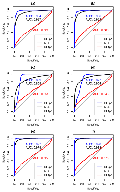
Figure 2: ROC Curves comparing Bayesian testing methods, for scenarios with $p_{s}=0.15$. Figures in the left column (a, c, and e) use the permuted null scenario data as the true-negatives, whereas figures in the right column (b, d, and f) use the all-or-none null data. Figures in the first row (a, b) use the $I_{E}=0.2$ (non-replacement-only) scenario data as the true-positives, whereas figures in the second (c, d) and third (e, f) rows use the insert-only and replacement-only $I_{E}=0$ scenario data, respectively.

For this example data, the Fisher’s exact test performed well for detecting moderate-sized sieve effects. The Gilbert, Wu, Jobes non-parametric t-test, evaluated using the HIV-b substitution matrix, performed relatively poorly in comparison to the other methods, particularly for the scenarios in which the non-insert distribution matters (all but the “insert-only” scenarios). GWJ performs particularly well for the insert-only scenarios because the HIV-b weight matrix strongly differentiates the target category from the untargeted categories, but doesn’t differentiate much among the untargeted categories (so the GWJ test with this matrix approximates a dichotomized Fisher test, little influenced by the distribution of the untargeted categories).

The new approaches outshine GWJ and Fisher for low $p_{s}$ values (see $p_{s}=0.15$ results for $I_{E}=0$ and $I_{E}=0.2$) when the non-insert distribution matters. In practice, the new methods can be seen as a complement to the routinely-used GWJ method, and can aptly be described as being more sensitive than GWJ to differences among non-targeted categories.

3.2 STEP

The sieve analysis of the breakthrough infections in the STEP (HVTN 502) HIV-1 vaccine trial identified a strong sieve effect at site Gag 84 (Rolland). Because the STEP vaccine was designed to elicit T cell responses that target HIV-1 after infection, it is reasonable in this case to consider a replacement-only model. Since the estimated vaccine efficacy was negative, this analysis should be viewed with caution as the SNL “no-harm” condition may not hold. The upcoming sieve analysis of the HVTN 505 HIV-1 vaccine efficacy trial, which was recently halted to new enrollments due to a finding of efficacy futility, will be a better example of a zero-efficacy setting. We present this analysis of HVTN 502 infections as a demonstration of how the SNL methods could be applied to HVTN 505 or similar settings.

Table 3.2 depicts the failure types observed at site Gag 84 among STEP participants who experienced HIV-1 infections during the trial. The sieve effect is so strong that power differences among testing procedures are not relevant. We can easily detect this effect, for instance, with a Fisher’s exact test (p = 0.001).

Table 2: STEP failure types at site Gag 84 and RV144 non-failure counts (labeled “0”) and failure types at site Env 169

	Gag 84			Env 169
	T	V		0	K	Q	R	E	T	V
V	8	31		7909	30	9	2	1	1	1
P	17	9		7914	57	7	2	0	0	0

Investigating these data with a two-phase analysis comparing the one-or-none model to the all-or-none model, we compute the log-likelihood ratio as -16.5, which has an (analytic) p-value of 9.3e-09, strongly supporting the one-or-none model over the all-or-none model at this site. To take a more conservative approach, we permute the treatment labels as described above, to estimate a null distribution that conditions on the marginal totals. Since none of these $1000$ permuted-data -2*LLRs was as large as the observed value of 32.99, we estimate the p-value as $p<0.001$, again supporting a sieve effect.

Figure 3: Two-phase hierarchical one-or-none evaluation of STEP site Gag 84: The approximate posterior distribution of $p_{s}$, evaluated using 1000 Monte Carlo simulations per point. The Y axis is log-scaled and unnormalized. The posterior mass is concentrated well above zero, which since $I_{E}=0$ indicates evidence for a sieve effect.

Now we turn to a Bayesian approach. Figure 3 shows the approximate posterior distribution of $p_{s}$ at this site when employing a hierarchical two-phase Bayesian approach (in which we use the placebo-recipient data to update priors on both $\bm{q}$ and $\bm{p_{c}}$). The posterior-maximizing value of $p_{s}$ is 0.68, which we could interpret as indicating that about two-thirds of the intervention recipients who became HIV-1 infected experienced immune escape at this locus that they would not have experienced in the absence of the intervention. Since this analysis depends on the no-harm assumption, this interpretation should be made cautiously.

3.3 RV144

The sieve analysis of the breakthrough infections in the RV144 HIV-1 vaccine trial identified a moderate sieve effect at site Env 169 (v2sieve). The trial had an estimated intervention efficacy of 31% overall, so unlike the STEP analysis, here we need not assume a replacement-only model. Table 3.2 depicts the failure types observed at site Env 169 among the 109 RV144 participants who experienced infections during the trial by subtype AE (CRF-01) HIV-1 viruses. The effect is weaker at this site, so power differences between testing procedures are relevant. We would not detect this effect, for instance, with a Fisher’s exact test (p = 0.089).

We now investigate this site using the dichotomous-take SNL framework, with a two-phase analysis comparing the one-or-none model to the all-or-none model. We compute the two-phase log-likelihood ratio as -31.95, which has an (asymptotic) p-value of 1.3e-15, indicating strong evidence supporting a sieve effect. Since $I_{E}>0$, we do not expect Wilks’s theorem to apply under the null. To take a more conservative approach, we permute the treatment labels to estimate a null distribution. Three of the $1000$ permuted-data $-2\otimes$LLRs were larger than the observed value of 63.9, so this result is much less significant than when employing the chi-squared null.

Now we turn to a Bayesian approach. We estimate the hierarchical (for both $\bm{p_{c}}$ and $\bm{q}$) two-phase Bayes factor at this site to be 3.1e+10, which is much greater than $1$ and thus supports the one-or-none model over the all-or-none model. In Figure 4 we investigate the posterior distribution of $p_{s}$ at RV144 site Env 169.

Figure 4: Two-phase hierarchical one-or-none evaluation of RV144 site Env 169: The approximate posterior distribution of $p_{s}$, evaluated using 1000 Monte Carlo simulations per point. The Y axis is log-scaled and unnormalized. The posterior mass is concentrated near $p_{s}=0.24$, indicating that about that fraction of the partial efficacy of RV144 can be attributed to the sieve effect.

The posterior-maximizing value of $p_{s}$ is 0.24, which we interpret as indicating that about one-quarter of the intervention recipients who became HIV-1 infected would not have become infected if the intervention had targeted all amino acids at site Env 169 rather than just the insert AA. That is, the HIV-1 infecting these subjects was able to escape the vaccine-induced immune pressure because the intervention targeted just the K, not the other AAs, at site Env 169. This analysis suggests that the incompleteness of the efficacy can only partly be attributed to the sieve effect. In this non-replacement-only case, the sieve effect strength is not simply equivalent to the rate of “take”; as discussed in section 2.7, the interpretation is that incomplete “take” accounts for $1-p_{s}$ (about three-quarters) of the unavoided vaccine-recipient failures, indicating that even if the vaccine had induced (in takers) immune responses that successfully targeted all amino acids at Env 169, the vaccine would still have been only partially efficacious (efficacy would have been about 50% rather than 31%).

4 Discussion

We have introduced a framework for sieve analysis of non-leaky interventions that do not cause harm (the intervention induces only “failure avoidance”, not new failures except as replacements of avoided failures). The framework provides a useful platform for reasoning about sieve effects, and we argue that apparent sieve effects are not generally attributable to actual differential efficacy across failure types except under either the “leaky” conditions of GSA, or under the no-harm, non-leaky conditions of this framework.

We have introduced models for evaluating sieve effects in this sievey-not-leaky setting. We have implemented both frequentist and Bayesian procedures, and we have demonstrated the power of both frequentist and Bayesian-frequentist hybrid approaches under various conditions. The primary parameter of the model, the “sieve effect strength” $p_{s}$, has the useful interpretation that it reflects the amount of an intervention’s partial efficacy that can be attributed to the sieve effect (as opposed to incomplete “take” of the intervention by some intervention recipients).

For replacement-only ($I_{E}=0$) scenarios, since the all-or-none model is nested in any some-or-none model whenever $p_{s}=0$, the hypothesis test based on likelihood ratios has a simple asymptotic analytic form. We found in our simulation experiments that the same analytic approach works well for scenarios with $I_{E}>0$ (to which the asymptotics do not apply).

The SNL framework that we have introduced is generalizable beyond the dichotomous “take” assumptions that we have employed here. At the extreme, we could allow non-zero probabilities for all of the $2^{J}$ possible response types allowed by the some-or-none framework (these index the set of types that are targeted, including both “all” and “none”). One particular example would constrain these to ensure independent “take” probabilities for each targeted type. It remains for future work to develop models and tests for this scenario.

With now two sieve analysis frameworks for two extremes of the spectrum (leaky interventions with 100% “take” and this new approach for non-leaky interventions with partial “take”), there remains a need for development of methods that support unbiased evaluation of sieve effects under conditions of both leaky and incomplete-take interventions. In the mean time, or if that is not possible, there remains a need for further development of tests to evaluate the conditions under which these methods yield reliable results.

We conclude with a brief discussion of the “no-harm” assumption. Mathematically, the no-harm condition requires that the per-exposure probabilities of infection are always $1$ under the control (or counterfactual or no-take) intervention scenario. This means that “exposure” is equated with “an exposure that would result in infection in the absence of the treatment intervention.” Here, the definition of “exposure” reflects a modeling choice that determines the tradeoff between the per-exposure probabilities and the exposure distributions.

For partially effective interventions, the choice may be arbitrary, but it is clearly not a reasonable assumption for an intervention with a significantly negative estimated efficacy. In such scenarios, it may still be possible to use the sievey-not-leaky failure avoidance framework by considering the control intervention an alternative treatment, and supposing a shared set of would-be-first failures (in a no-harm setting) that are avoided at different rates by the two interventions. We leave this to future work.