Meta-analysis of functional neuroimaging data using Bayesian nonparametric binary regression

Abstract

In this work we perform a meta-analysis of neuroimaging data, consisting of locations of peak activations identified in $162$ separate studies on emotion. Neuroimaging meta-analyses are typically performed using kernel-based methods. However, these methods require the width of the kernel to be set a priori and to be constant across the brain. To address these issues, we propose a fully Bayesian nonparametric binary regression method to perform neuroimaging meta-analyses. In our method, each location (or voxel) has a probability of being a peak activation, and the corresponding probability function is based on a spatially adaptive Gaussian Markov random field (GMRF). We also include parameters in the model to robustify the procedure against miscoding of the voxel response. Posterior inference is implemented using efficient MCMC algorithms extended from those introduced in Holmes and Held [Bayesian Anal. 1 (2006) 145–168]. Our method allows the probability function to be locally adaptive with respect to the covariates, that is, to be smooth in one region of the covariate space and wiggly or even discontinuous in another. Posterior miscoding probabilities for each of the identified voxels can also be obtained, identifying voxels that may have been falsely classified as being activated. Simulation studies and application to the emotion neuroimaging data indicate that our method is superior to standard kernel-based methods.

, and au1Supported by a PSC-CUNY Award, jointly funded by the Professional Staff Congress and the City University of New York. au2Supported in part by NSF Grant DMS-08-06088.

1 Introduction

1.1 Meta-analysis of neuroimaging studies

In recent years there has been a rapid increase in the number and variety of neuroimaging studies being performed around the world. This growing body of knowledge is accompanied by a need to integrate research findings and establish consistency across labs and scanning procedures, and to identify consistently activated regions across a set of studies. Performing meta-analyses has become the primary research tool for accomplishing this goal [Wager, Lindquist and Kaplan (2007); Wager et al. (2009)]. Evaluating consistency is important because false positive rates in neuroimaging studies are likely to be higher than in many fields, as many studies do not adequately correct for multiple comparisons. Thus, some of the reported activated locations are likely to be false positives, and it is important to assess which findings have been replicated and have a higher probability of being real activations. Individual imaging studies often use very different analyses [see Lindquist (2008) for an overview], and effect sizes are only reported for a small number of activated locations, making combined effect-size maps across the brain impossible to reconstruct from published reports. Instead, meta-analysis is typically performed on the spatial coordinates of peaks of activation (peak coordinates), reported in the standard coordinate systems of the Montreal Neurologic Institute (MNI) or Talairach and Tournoux (1988), and combined across studies. These peak coordinates typically correspond to the voxel whose $t$-statistic takes the maximum value in a spatially coherent cluster of activation, that is, the max statistic among a set of adjacent voxels that exceed a certain threshold. This information is typically provided in most neuroimaging papers and simple transformations between the two standard spaces exist.

A typical neuroimaging meta-analysis studies the locations of peak activations from a large number of studies and seeks to identify regions of consistent activation. This is usually performed using kernel-based methods such as activation likelihood estimation [ALE; Turkeltaub et al. (2002)] or kernel density approximation [KDA; Wager, Jonides and Reading (2004)]. In both methods, maps are created for each study by convolving an indicator map, consisting of an impulse response at each study peak, with a kernel of predetermined shape and width. The resulting maps are thereafter combined across studies to create a meta-analysis map. Monte Carlo methods are used to find an appropriate threshold to test the null hypothesis that the $n$ reported peak coordinates are uniformly distributed throughout the grey matter. A permutation distribution is computed by repeatedly generating $n$ peaks at random locations and performing the smoothing operation to obtain a series of statistical maps under the null hypothesis that can be used to compute voxel-wise $p$-values. The two approaches differ in the shape of the smoothing kernel. In KDA, it is assumed to be a sphere with fixed radius, while in ALE it is a Gaussian with fixed standard deviation.

A major shortcoming of kernel-based approaches is that the width of the kernel, and thus the amount of smoothing, is fixed a priori and assumed to be constant throughout the brain. In order to address these concerns, we propose a fully Bayesian nonparametric binary regression method for performing neuroimaging meta-analysis. In our method, each location has a probability of being a peak activation, and the corresponding probability function is based on a spatially adaptive Gaussian Markov random field (GMRF). The locally adaptive features of our method allows us to better match the natural spatial resolution of the data across the brain compared to using an arbitrary chosen fixed kernel size.

Figure 1: Example of the raw data are shown for a representative sagittal, coronal and axial slice of the brain. Each point represents a reported activation foci in an individual study by criteria designated by that particular study. All foci are reported and plotted in the MNI brain template to allow for cross study comparisons.

In this work, a meta-analysis was performed on the results of $162$ neuroimaging studies ($57$ PET and $105$ fMRI) on emotion. The studies were all performed on healthy adults and published between 1990 and 2005. For each study, the foci of activation were included when reported as significant by the criteria designated in the individual studies. Relative decreases in activation in emotion related tasks were not analyzed. All coordinates were reported on the MNI coordinate system to allow for cross study comparisons. Together, these studies yield a data set consisting of $2478$ unique peak coordinates. This data set is described in greater detail in Kober et al. (2008). Due to the relative scarcity of neuroimaging studies on a particular topic (e.g., emotion), it is standard practice in meta-analysis to combine data obtained using different imaging modalities, sample sizes and statistical analyses. This is done to ensure that the analysis has enough power to detect effects of interest. In addition, studies in Wager et al. (2008) have shown no significant difference between MRI and PET in the assessment of their functional maps and their foci of activation. Figure 1 shows the raw data for representative slices of the brain with fixed $x$, $y$ and $z$ directions, respectively. Each point in the plot represents the location of the peak of a cluster of reported activation from one of the $162$ neuroimaging studies. The primary goal for analyzing this data set was to determine areas of the brain that are consistently active in studies of emotion.

1.2 Statistical modeling for binary response

Let $Y$ be a random binary response variable, $X$ a vector of covariates and $p(\mathbf{x})$ the response probability function, $p(\mathbf{x})=\operatorname{Pr}(Y=1|X=\mathbf{x})$. In the context of fMRI meta-analysis, $Y=1$ if the voxel is reported as being a peak activation. The vector $X$ includes the voxel location and possibly other covariates related to the patient or the study. In nonparametric binary regression, we have $p(\mathbf{x})=H(z(\mathbf{x}))$, where $H$ is a specified cumulative distribution function often referred to as the link function. Popular link functions are the standard logistic and standard normal cumulative density functions.

The traditional parametric approach to binary regression involves setting $z(\mathbf{x})=\alpha+\bm{\beta}^{T}\mathbf{x}$, with unknown parameters $\alpha$ and $\bm{\beta}$. McCullagh and Nelder (1989) contains a comprehensive treatment of frequentist parametric methods with exponential family models, binary regression being a special case. Bayesian binary regression is well documented in, for example, Dey, Ghosh and Mallick (2000). In particular, Albert and Chib (1993) and Holmes and Held (2006) introduced auxiliary variable methods that provide efficient Markov chain Monte Carlo (MCMC) inference for parametric binary regression.

There is an extensive non-Bayesian literature on nonparametric regression using exponential family models, with binary regression treated as a special case. O’Sullivan, Yandell and Raynor (1986) estimated a single function using a penalized likelihood approach, and their work was extended to additive models by Hastie and Tibshirani (1990). Gu (1990) and Wahba et al. (1995) used tensor product smoothing splines to allow for interactions between variables and estimated smoothing parameters via a generalized cross-validation technique. Loader (1999) proposed a local likelihood approach for both univariate and bivariate nonparametric estimation and provided data-driven bandwidth estimators.

Bayesian methods for nonparametric binary regression were developed in Wood and Kohn (1998), Holmes and Mallick (2003), Choudhuri, Ghosal and Roy (2007), and Trippa and Muliere (2009). These methods are not locally adaptive, however. Krivobokova, Crainiceanu and Kauermann (2008) proposed an adaptive penalized spline estimator for binary regression based on quasi-likelihoods. Wood et al. (2008) presented a locally adaptive Bayesian estimator for binary regression by using a mixture of probit regressions where the argument of each probit regression is a thin-plate spline prior with its own smoothing parameters and the mixture weights depend on the covariates.

In fMRI meta-analysis, kernel-based smoothing techniques are typically used to identify regions of consistent activation and Monte-Carlo procedures are used to establish statistical significance. These techniques count the number of activation peaks within a radius of each local brain area and compare the observed number to a null distribution to establish significance. The kernel radius is chosen by the analyst, and kernels that match the natural spatial resolution of the data are the most statistically powerful [Wager, Lindquist and Kaplan (2007)]. In our method, the function $z(\cdot)$ is assumed to be a spatially adaptive Gaussian Markov random field (GMRF) with locally varying variance. The local adaptiveness of the procedure allows the probability function to be smooth in some regions and wiggly in others, depending on the data information. The need of adaptive smoothing for fMRI data has been demonstrated in Brezger, Fahrmeir and Hennerfeind (2007) and Yue, Loh and Lindquist (2010). The proposed Bayesian nonparametric binary regression method is an extension to the binary response case of methods developed in Yue and Speckman (2010) and Yue and Loh (2011). To make this procedure better suited for application to fMRI meta-analysis, we incorporate additional model parameters associated with the probabilities of voxels being miscoded. This makes the modeling more robust to possible errors in the data. The posterior inference is carried by efficient MCMC algorithms extended from those in Holmes and Held (2006). From the model fit we obtain a map of the probability of observing a peak activation across the brain as well as posterior miscoding probabilities. Regions of the brain with high probability estimates are identified as activated based on the meta-analysis. This makes the proposed method far more interpretable than earlier approaches.

The rest of the paper is organized as follows. The proposed method is described in Section 2. Section 3 presents simulation studies comparing our method to other available methods. Results of the data analysis are given in Section 4. Section 5 concludes this work with discussions.

2 Bayesian hierarchical modeling and inference

We describe in this section our nonparametric binary regression model using the spatially adaptive GMRF. Note that our method currently can only be implemented in two dimensions. We apply it to the fMRI setting by fitting the model to brain slices in succession. This is similar to the staggered approach in Penny, Trujillo-Barreto and Friston (2005), who used a two-dimensional Laplacian prior that is related to our GMRF prior.

2.1 Spatially adaptive GMRF on regular lattice

Let us denote by $\mathbf{x}=(x_{11},x_{21},\ldots,x_{n_{1},n_{2}})^{\prime}$ an $n$-dimensional vector of voxel locations on a regular $n_{1}\times n_{2}$ lattice ($n=n_{1}n_{2}$). Adopting notation $z_{jk}=z(x_{jk})$, we assume that the underlying spatial process $z_{jk}$ is an adaptive Gaussian Markov random field (GMRF) as introduced in Yue and Speckman (2010). This adaptive GMRF is based on the following spatial Gaussian random walk model:

$$\bigl{(}\nabla^{2}_{(1,0)}+\nabla^{2}_{(0,1)}\bigr{)}z_{jk}\sim\mathrm{N}(0,\delta^{2}\gamma_{jk}^{2}),$$ (1)

where $\nabla^{2}_{(1,0)}$ and $\nabla^{2}_{(0,1)}$ denote the second-order backward difference operators in the vertical and horizontal directions respectively, that is, $\nabla^{2}_{(1,0)}z_{jk}=z_{j+1,k}-2z_{jk}+z_{j-1,k}$ and $\nabla^{2}_{(0,1)}z_{jk}=z_{j,k+1}-2z_{jk}+z_{j,k-1}$ for $2\leq j\leq n_{1}-1$ and $2\leq j\leq n_{2}-1$. The parameter $\delta^{2}$ is a global smoothing parameter accounting for large-scale spatial variation while $\gamma_{jk}^{2}$ are the adaptive smoothing parameters that capture the local structure of the process $z(\mathbf{x})$. The equation (1) essentially defines an adaptive smoothness prior on the second-order difference $(\nabla^{2}_{(1,0)}+\nabla^{2}_{(0,1)})z_{jk}$. As a result, the conditional distribution of each $z_{jk}$ given the rest $\mathbf{z}_{-jk}$ is Gaussian and only depends on its neighbors in a specific way. This dependence can be shown using a graphical notation by expressing the conditional expectation of an interior $z_{jk}$ as

$$E(z_{jk}|\mathbf{z}_{-jk})=\frac{1}{20}\left(8\begin{array}[]{ccccc}\circ&\circ&\circ&\circ&\circ\\[-6.0pt] \circ&\circ&\bullet&\circ&\circ\\[-6.0pt] \circ&\bullet&\circ&\bullet&\circ\\[-6.0pt] \circ&\circ&\bullet&\circ&\circ\\[-6.0pt] \circ&\circ&\circ&\circ&\circ\end{array}-2\begin{array}[]{ccccc}\circ&\circ&\circ&\circ&\circ\\[-6.0pt] \circ&\bullet&\circ&\bullet&\circ\\[-6.0pt] \circ&\circ&\circ&\circ&\circ\\[-6.0pt] \circ&\bullet&\circ&\bullet&\circ\\[-6.0pt] \circ&\circ&\circ&\circ&\circ\end{array}-1\begin{array}[]{ccccc}\circ&\circ&\bullet&\circ&\circ\\[-6.0pt] \circ&\circ&\circ&\circ&\circ\\[-6.0pt] \bullet&\circ&\circ&\circ&\bullet\\[-6.0pt] \circ&\circ&\circ&\circ&\circ\\[-6.0pt] \circ&\circ&\bullet&\circ&\circ\end{array}\right),$$ (17)

where the locations denoted by a “$\bullet$” represent those values of $\mathbf{z}_{-jk}$ that the conditional expectation of $z_{jk}$ depends on, and the number in front of each grid denotes the weight given to the corresponding “$\bullet$” locations. Therefore, the conditional mean of $z_{jk}$ is a particular linear combination of the values of its neighbors, and its conditional variance is $\operatorname{Var}(z_{jk}|\mathbf{z}_{-jk})=20\delta^{2}\gamma_{jk}^{2}$.

The use of $\gamma_{jk}^{2}$ is important for estimating activation probabilities in a fMRI meta-analysis. To identify consistently activated regions across a set of studies, we need less smoothing (large $\gamma_{jk}^{2}$) where there are many reported peak locations and relatively more smoothing (small $\gamma_{jk}^{2}$) where very few or no peaks are reported. Standard smoothing techniques (e.g., kernel smoother with fixed width) suffer from a trade-off between increased detectability and loss of information about the spatial extent and shape of the activation areas. Adaptive smoothing provided by $\gamma_{jk}^{2}$ can reduce such loss of information. The need of adaptive smoothing for processing fMRI imaging data was also demonstrated in Brezger, Fahrmeir and Hennerfeind (2007) and Yue, Loh and Lindquist (2010). Note that setting $\gamma_{jk}^{2}\equiv 1$ makes (1) a nonadaptive GMRF on lattice, yielding a Bayesian solution for thin-plate splines [see Rue and Held (2005), section 3.4.2].

Additional priors need to be specified for $\gamma_{jk}^{2}$ in (1). We use independent inverse gamma priors for $\gamma^{2}_{jk}$, that is, $\gamma_{jk}^{-2}\stackrel{{\scriptstyle\mathrm{i.i.d.}}}{{\sim}}\operatorname{Gamma}(\nu/2,1/2),\nu>0$. The marginal prior distribution of the increment in (1) turns out to be a Student-$t$ distribution with $\nu$ degrees of freedom. We choose a Cauchy distribution ($\nu=1$), which has been suggested as a default prior for robust nonparametric regression [Carter and Kohn (1996)] and sparse Bayesian learning [Tipping (2001)]. Yue and Loh (2011) and Brezger, Fahrmeir and Hennerfeind (2007) also suggested similar priors for $\gamma^{2}_{jk}$ in their work on adaptive spatial smoothing. Yue and Speckman (2010) and Yue, Loh and Lindquist (2010), however, assumed another spatial GMRF model for $\log(\gamma^{2}_{jk})$ in a second hierarchy. Although it has been applied successfully for modeling spatial data, this two-stage GMRF prior forces the $\gamma_{jk}^{2}$ to be smooth and it is not suitable for estimating spatial processes with jumps or sharp peaks. Furthermore, the computation is rather complicated, precluding extensions to more flexible regression models, for example, the binary hierarchical regression model considered here.

The prior for $\delta^{2}$ is often chosen to be a conjugate diffuse but proper inverse gamma prior. We, however, propose to use a half-$t$ distribution as the prior for its square root, that is,

$$[\delta|\rho,S]\propto\biggl{(}1+\frac{1}{\rho}\biggl{(}\frac{\delta}{S}\biggr{)}^{2}\biggr{)}^{-(\rho+1)/2},\qquad\delta>0,$$ (18)

where $\rho$ is the parameter of degrees of freedom and $S$ is the scale parameter. The half-$t$ distribution can be treated as the absolute value of a Student-$t$ distribution centered at zero [see Psarakis and Panaretos (1990)]. Although it is not commonly used in statistics, the half-$t$ distribution was used in objective Bayesian inference by Wiper, Girón and Pewsey (2008) and suggested for use as a default prior for a variance component in hierarchical models [e.g., Gelman (2006); Gelman et al. (2008)]. This family includes, as special cases, the improper uniform density (if $\rho=-1$) and the proper half-Cauchy (if $\rho=1$). Following Carvalho, Polson and Scott (2010), we use a standard half-Cauchy prior ($\rho=S=1$) due to its heavy tail and substantial mass around zero. Although it is not conjugate, the half-$t$ prior on $\delta$ can be written as $\delta\stackrel{{\scriptstyle\mathcal{D}}}{{=}}|\xi|\theta$, where $\xi\sim\mathrm{N}(0,1)$ and $\theta^{2}\sim\operatorname{IG}(\rho/2,\rho S^{2}/2)$ [e.g., Psarakis and Panaretos (1990)]. This property enables us to develop efficient MCMC sampling schemes as shown in the Appendix.

2.2 Posterior inference

Although any cumulative distribution function (cdf) $H$ that preserves the smoothness of $\mathbf{z}$ may be used as a link function, here, we only consider the case in which the $H$ can be represented as the scale mixture of mean zero normal cdf’s. Two special examples are the well-known probit and logit link functions. With a specific link function, the posterior distribution of $\mathbf{z}$ is not analytically tractable, and thus an MCMC algorithm will be used to compute the posterior distribution. The algorithm is based on the auxiliary variable method in Holmes and Held (2006) and GMRF simulation techniques in Rue and Held (2005). Briefly, the data are augmented by introducing an auxiliary variable $w_{i}$ that follows a normal distribution with mean $z_{i}$ and variance $\lambda_{i}$. The new data $w_{i}$ are associated with original binary data $y_{i}$ in the following way: $y_{i}=1$ if $w_{i}>0$ and $y_{i}=0$ if $w_{i}\leq 0$. Then, the adaptive GMRF prior is taken on $z_{i}$ and a certain prior distribution chosen for $\lambda_{i}$ depending on the link function. The full conditional distributions for the Gibbs sampler are all easily derived and can be efficiently sampled. In the Appendix we provide the detailed MCMC algorithms for the link functions that are the probit, logit and general scale mixture of normals.

2.3 Robustification

In this section we describe how to robustify our procedure against miscoding of the response variable. Adopting the idea in Choudhuri, Ghosal and Roy (2007), we use indicator variables $\bm{\psi}=(\psi_{1},\ldots,\allowbreak\psi_{n})^{\prime}$ such that $\psi_{i}=1$ indicates that $y_{i}$ is miscoded and $\psi_{i}=0$ indicates that $y_{i}$ is correctly coded. In the context of fMRI meta-analysis, $\psi_{i}=1$ means that $y_{i}$ is either a false positive or a false negative. Since these variables cannot be observed, we treat them as unknown parameters that need to be estimated via taking priors on them. The joint posterior distribution of $(\bm{\psi},\mathbf{z})$ is then used to obtain a robust estimate of $\mathbf{z}$, and also to identify the miscoded observations.

We assume that each observation has equal probability of being miscoded, independent of other observations and $\mathbf{z}$. Denote by $r$ an a priori guess for the probability of an observation being miscoded. Given $(\bm{\psi},\mathbf{z})$, the $y_{i}$’s are independent Bernoulli random variables with probability of success $(1-\psi_{i})H(z_{i})+\psi_{i}(1-H(z_{i}))$. As a result, the conditional distributions of $\psi_{i}$ are independent with

$$P(\psi_{i}=1|\mathbf{y},\mathbf{z})=\cases{\displaystyle\frac{r[1-H(z_{i})]}{r[1-H(z_{i})]+(1-r)H(z_{i})},&\quad if $y_{i}=1$,\vspace*{3pt}\cr\displaystyle\frac{rH(z_{i})}{rH(z_{i})+(1-r)[1-H(z_{i})]},&\quad if $y_{i}=0$.}$$ (19)

Consider the probit link without any hyperprior. As shown in Section .1, we adjust latent variables $w_{i}$ for miscoding, that is, $y_{i}=1$ if $\{w_{i}>0,\psi_{i}=0\}$ or $\{w_{i}<0,\psi_{i}=1\}$. Then,

$$(w_{i}|\bm{\psi},\xi,\bm{\eta},\mathbf{y})\sim\cases{\displaystyle\mathrm{N}(\xi\eta_{i},1)I(w_{i}>0),&\quad if $y_{i}+\psi_{i}=1$,\cr\displaystyle\mathrm{N}(\xi\eta_{i},1)I(w_{i}\leq 0),&\quad if $y_{i}+\psi_{i}\neq 1$.}$$ (20)

Hence, samples from the joint distribution $(\psi_{i},w_{i}|\mathbf{z},\mathbf{y})$ can be drawn by first sampling $\psi_{i}$ using (19) and then sampling $w_{i}$ using (20). Since the full conditional of $\mathbf{z}$ does not depend on $\bm{\psi}$ or $\mathbf{y}$, the samples from the conditional distributions of the rest of the parameters can be drawn as described earlier. Note that the algorithm of this robust approach may be extended similarly to the logit link or an arbitrary symmetric link by introducing the relevant latent variables.

(a)	(b)
(c)	(d)

Figure 2: Simulation I: (a) True probability function; (b) Estimated probability function using proposed method with probit link; (c) Estimated probability function using FAPS method; (d) Mean squared probability errors using proposed method and FAPS method.

3 Simulation studies

We performed two different types of simulation studies to investigate the performance of our method. The first simulation is in the setting of nonparametric binary regression, where the proposed method is compared to an adaptive penalized spline model. The second simulation is in the setting of fMRI meta-analysis, where our method is compared to the kernel-based ALE method, which is commonly used in neuroimaging meta-analysis.

3.1 Simulation I

The true probability function is assumed to be

$$p(\mathbf{x})=\Phi\biggl{\{}6\exp\biggl{[}-\frac{5}{2}\bigl{(}(x_{1}-2)^{2}+(x_{2}-2)^{2}\bigr{)}\biggr{]}+3\exp\biggl{[}-\frac{1}{10}(x^{2}_{1}+x_{2}^{2})\biggr{]}-3\biggr{\}}.$$

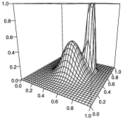
It is a smooth bimodal spatial surface on a $30\times 30$ regular lattice as shown in Figure 2(a). One hundred data sets were simulated and we use the mean squared probability error (MSPE),

$$\mathrm{MSPE}=\frac{1}{n}\sum_{i=1}^{n}\{p(\mathbf{x}_{i})-\hat{p}(\mathbf{x}_{i})\}^{2},$$

to measure performance, where $\hat{p}(\cdot)$ is the estimated probability function.

The estimates obtained using our Bayesian nonparametric binary regression model are compared to those obtained using the fast adaptive penalized splines (FAPS) model in Krivobokova, Crainiceanu and Kauermann (2008). The FAPS approach models the regression function as a penalized spline with a smoothly varying smoothing parameter function which is also modeled as a penalized spline. Their method handles local smoothing of binary data as a special case. The authors showed that the FAPS estimator outperformed the penalized spline estimators in Crainiceanu et al. (2007) and Ruppert and Carroll (2000). The model can be fit using the AdaptFit R package.

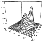
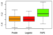
Panels (b) and (c) in Figure 2 show typical fits for the bimodal function using our method and FAPS method, respectively. It appears that the FAPS model has difficulty capturing the sharp peak and undersmoothes the flat portion as well. Figure 2(d) shows the distributions of the MSPE produced by those two methods, where the FAPS estimator is apparently outperformed. Also, in our method the two link functions yield similar performances in terms of MSPE. This is because nonparametric modeling of $\mathbf{z}$ makes the model robust against the choice of the link function. We believe that the underperformance of FAPS stems from using slowly varying functions to model local smoothing parameters. Although they provide computational efficiency, such low-rank basis functions are unable to capture sharp changes in the function. Yue and Speckman (2010) presented similar results for normal response variables. Note that the robustification procedure is not required in this simulation study.

Figure 3: (A) The probability map used to generate random activation peaks; (B) One set of simulated activation peaks.

3.2 Simulation II

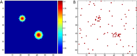
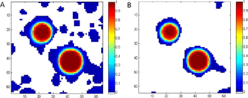
In the second simulation study we began by constructing a $64\times 64$ probability map, denoted $p(x,y)$, where the value at each voxel location $(x,y)$ represents the probability that it be recorded as a “peak coordinate” in a neuroimaging study. The probability map consisted of two circular regions of heightened probability (see Figure 3A), where the maximum probability is roughly $0.4$. Voxels lying outside these two regions were set to have a constant background probability of $0.01$, thus allowing for the possibility of “false positives” outside the two centers of activation. Next, the probability map was used to generate random activation peaks. The voxel at coordinate $(x,y)$ was considered a reported peak according to a binomial distribution with probability of activation $p(x,y)$. This process was repeated $100$ times and each time gives rise to simulated meta-analysis data. Figure 3B shows the data for one repetition. The data shows clear clustering around the two regions of activation, while still allowing for spurious activations in the rest of the image. This corresponds with the behavior of standard meta-analysis data (see, e.g., Figure 1).

Figure 4: Proportion of times each voxel was deemed significant at the $5\%$ level (A) and the $1\%$ level (B) using the ALE method.

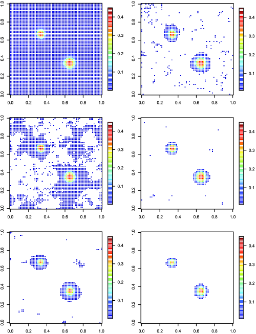
Each of the $100$ repetitions were analyzed using the kernel-based ALE method as well as our Bayesian nonparametric binary regression model. In the former, a kernel with bandwidth $10\mbox{ mm}$ full width at half maximum (FWHM) was used, as this is the standard in the field. A Monte Carlo procedure was used to determine the appropriate threshold to test the null hypothesis that the reported peak coordinates are uniformly distributed throughout the grey matter. A permutation distribution is computed by repeatedly generating peaks at random locations and performing the smoothing operation to obtain a series of statistical maps under the null hypothesis that can be used to determine which voxels had $p$-values below $\alpha$, where $\alpha$ was set to $0.05$ and $0.01$. Regarding our Bayesian method, the robustification procedure described in Section 2.3 is implemented since we use the background probability of 0.01 to produce the false positives. To see how sensitive the results are to the use of robustification, we fit the model with prior miscoding probability $r=0$ (no robustification), $r=0.01$ and $r=0.05$. Figures 4A and B show the proportion of times each voxel was deemed significant at the $5\%$ level and the $1\%$ level, respectively, in the $100$ repetitions, when the ALE method was used. It is clear that the kernel smoother does a very good job of finding true positives, but tends to have a large number of false positives in the area immediately surrounding the activated regions. Figure 5 shows the average probability of activation in each voxel obtained using our method. The maps in the left column are not thresholded, while those in the right column are thresholded at 0.01. Apparently, our estimates are closer to the simulated probability map and produce much fewer false positives than the kernel estimates. Furthermore, our method yields fewer false positives as the value of $r$, the prior miscoding probability, increases, that is, the fit becomes more robust. The spatial extent of the activation region, however, is not significantly shrunk, making a strong case for the use of adaptive smoothing.

Figure 5: Average probability of activation in each voxel obtained using the adaptive GMRF method combined with the robustification procedure under different prior miscoding probabilities: $r=0$ (top row), $r=0.01$ (middle row) and $r=0.05$ (bottom row); The maps in the left column are not thresholded, while those in the right column are thresholded at 0.01.

Figure 6: Assessment of MCMC convergence for Simulation I. The top (bottom) two rows contain the typical trace plots and autocorrelation functions of the samples of variables $z$, $\gamma$ and $w$ from fitting a probit (logistic) model.

3.3 Computational performance and MCMC diagnostics

Thanks to the sparse structure of the adaptive GMRF prior used, the proposed models provide fast MCMC computation for nonparametric binary regression. To complete 5000 iterations on a 3.06 GHz Intel iMac desktop with 4GB memory, it took the probit model 9.23, 46.06 and 11.17 seconds at sample size $n=30\times 30$, $60\times 60$ and $90\times 90$, respectively, for estimating the bimodal function in Simulation I. The logistic model is a little slower, taking 11.89, 55.83 and 138.69 seconds to finish the same amount of computations. The computing times of both models increase with sample sizes at order $n$, roughly. The programs were written in the FORTRAN language, making use of the LAPACK and BLAS packages.

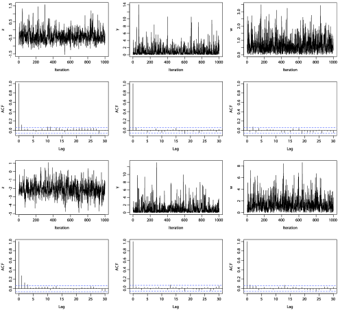
It is well known that the GMRF $\mathbf{z}$ are strongly dependent on each other as well as on the auxiliary variable $\mathbf{w}$ [see, e.g., Rue and Held (2005); Holmes and Held (2006)]. Those posterior correlations are likely to cause slow mixing in the Markov chain. To combat this issue, we sampled $\mathbf{z}$ as a block and employed the joint updating tricks as used in Holmes and Held (2006) (see the Appendix for details). Since the computation is fast, we also suggest running a relatively large number of MCMC iterations and applying a thinning factor of $\ell$ by collecting samples after every $\ell$ iterations. In Simulation I, for instance, we found that it is sufficient to run 15,000 MCMC iterations (5000 burn-in and 10,000 sampling) with a thinning factor of 10 to obtain reliable estimates. Figure 6 shows typical trace plots and autocorrelation functions of the samples of different variables for Simulation I. As we can see, the mixing of the chain is satisfactory for both probit and logistic models.

Figure 7: Assessment of MCMC convergence for the data analysis. The top row contains the typical trace plots of the samples of variables $z$, $\gamma$ and $w$; the bottom row contains the corresponding autocorrelation functions.

4 Data analysis

We describe here the results of our meta-analysis of the fMRI data. As mentioned before, the data consists of the coordinates of $2478$ peaks representing the locations of voxel activations, collected from 162 neuroimaging studies. The raw data consists of a three-dimensional image with dimensions $91\times 109\times 91$ whose elements took the value $1$ if an activation had been reported at that voxel and $0$ otherwise. Figure 1 shows the raw data for a representative slice of the brain with fixed $x$, $y$ and $z$ directions, respectively.

The binary nature of the meta-analysis data makes it an ideal candidate for our Bayesian nonparametric binary regression method. As our method is currently only implemented in two dimensions, we fit our method slice-wise across the brain for each orientation (i.e., for the fixed $x$, $y$ and $z$ direction). Prior to performing our method on a slice, we applied smoothing in the fixed direction by including all activations located within $10$ mm of the slice of interest.

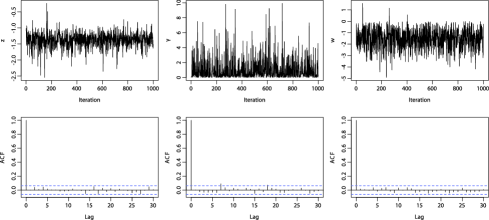
In our simulation studies (Section 3), we found that the binary regression model is not sensitive to the choice of link function. We therefore fit a probit model to the data for computational efficiency. To make our estimation robust against false positives, we incorporated the robustification procedure (Section 4) in the model with prior miscoding probability $r=0.01$ for every voxel. Due to the high dimension of the data, the MCMC was run for 60,000 iterations with 10,000 burn-in and a thinning factor of 50 iterations, resulting in posterior samples of size 1000. The Markov chains mix well as shown in Figure 7.

Figure 8: Thresholded posterior probability maps are shown for the sagittal, coronal and axial slice of the brain depicted in Figure 1. Regions with posterior probability of observing a peak activation higher than $0.30$ are color-coded.

Figure 9: Miscoding probabilities are shown for the sagittal, coronal and axial slice of the brain depicted in Figure 1. Points with posterior miscoding probability higher than $0.10$ are color-coded.

Once the Bayesian binary regression model was fit, posterior probability maps were obtained indicating the probability of being a location of peak activation across the brain. Regions with probability values higher than $0.3$ were color-coded and superimposed onto an anatomical reference image. The relatively low threshold is indicative of the dispersion of foci locations in the data. Figure 8 shows results for the three slices described above. Key regions of activation observed in the figure include the thalamus (8A), amygdala (8B) and the ventral striatum (8C). These regions are known to be associated with emotion, and were also indicated as active when using kernel-based methods [see Kober et al. (2008)]. It should be noted we obtain the same regions of activation as Kober et al. (2008), but with significantly smaller spatial extent. This is consistent with our simulation study, which shows how the kernel-based methods tend to overestimate the extent of activation. Finally, Figure 9 shows the posterior miscoding probabilities (thresholded at 0.10) for the same three slices. High miscoding probabilities indicate points that were deemed to be spurious activations and therefore given lower weights when calculating the posterior activation probabilities. Based on their locations, it appears that our method is providing an effective means of downweighting false activations.

To see if the adaptive smoothing is preferred to the ordinary smoothing in this neuroimaging example, we conducted a test on $H_{0}\dvtx\gamma_{jk}=1$ using the deviance information criterion (DIC) introduced by Spiegelhalter et al. (2002). More specifically, we first fitted to our imaging data the proposed adaptive GMRF model and a (nonadaptive) Bayesian thin-plate spline model (by fixing all $\gamma_{jk}$ to be 1), and saved the MCMC posterior samples of both models. Then, we define the deviance as $D(\bm{\phi})=-2\log(p(\mathbf{y}|\bm{\phi}))$, where $p(\mathbf{y}|\bm{\phi})$ is the likelihood function and $\bm{\phi}$ are unknown parameters of the model. The DIC score is finally estimated using $\mathit{DIC}=2\bar{D}-D(\bar{\bm{\phi}})$, where $\bar{D}$ is calculated as the average of $D(\bm{\phi})$ over the samples of $\bm{\phi}$, and $D(\bar{\bm{\phi}})$ as the value of $D$ evaluated at the average of the samples of $\bm{\phi}$. The model with smaller DIC should be in favor. Table 1 shows the DIC scores of the two models for the fixed $x$, $y$ and $z$ orientations, where the adaptive model is preferred in every scenario.

=217pt Orientation x y z Adaptive 0,9918.372 8216.255 9917.209 Nonadaptive 10,090.460 9512.016 9947.377

Table 1: DIC scores of both adaptive and nonadaptive models for the fixed $x$, $y$ and $z$ orientation.

5 Discussion

We developed a fully Bayesian method for nonparametric binary regression and, together with a robustification procedure, applied it to meta-analysis in fMRI studies. Our analysis identified activated regions of the brain that are known to be associated with emotion. While similar regions were also identified in other meta-analyses such as Kober et al. (2008) that use kernel-based methods, our method has several advantages over such approaches as follows. The adaptive GMRF used in our model better matches the natural spatial resolution of the data across the brain compared to using an arbitrary chosen fixed kernel size. This allows us to avoid the problem of overestimating regions of activation apparent in kernel-based methods. The Bayesian nature of our method allows for the construction of posterior probability maps indicating the probability of observing a peak activation in response to the paradigm across the brain. This is in contrast to kernel methods which simply state that more peaks lie near the voxel than expected by chance. It should be noted that recently a Bayesian spatial hierarchical model using a marked independent cluster process [Kang et al. (2011)] was introduced for dealing with neuroimaging meta-analysis. In future work we will look at comparing this method with the nonparametric binary regression approach suggested in this paper. Finally, our procedure provides estimates of miscoding probabilities which can help to identify regions that may have been incorrectly tagged as being activated. This is another feature not provided by kernel-based methods.

It is important to note that in this work the model setup assumes that the input data is two dimensional. Such 2D smoothing serves a useful purpose, as fMRI data are often analyzed either slice-wise or using cortical surface-based techniques [Dale, Fischl and Sereno (1999); Fischl, Sereno and Dale (1999)]. In reality, however, fMRI data are three dimensional in space. Therefore, it may ultimately be more appropriate to smooth the three spatial dimensions directly. We are actually working on such an extension of our current approach. The main computational constraint stems from inverting a large precision matrix, which is of $91\times 109\times 91=902{,}629$ dimensions in our neuroimaging example. We thus need a practical 3D GMRF, but the construction is nontrivial. One possible solution is to obtain a highly sparse precision matrix by discretizing a 3D Laplacian operator with proper boundary conditions as we did in the 2D case. To achieve more computational efficiency, we may use a novel Bayesian inference tool similar to that introduced in Rue, Martino and Chopin (2009) rather than MCMC.

As shown in the simulation studies, the results obtained by our method are somewhat sensitive to the prior miscoding probability $r$ in the robustification procedure. A large $r$ may underestimate the activation clusters, while a small $r$ tends to allow more false positives. The choice of $r$ is often subjective. One may use information from, say, previous studies, to find an appropriate $r$ in order to balance this trade-off. If no prior information is available, Choudhuri, Ghosal and Roy (2007) proposed letting $r$ be a small number between 0.01 and 0.1. In practice, we suggest experimenting with several $r$ values and choosing the one that gives the best results.

Appendix: MCMC algorithms for posterior inference

.1 Probit link

Let $\mathbf{y}=(y_{1},\ldots,y_{n})^{T}$ be the random vector of binary observations measured and $\mathbf{x}=(x_{1},\ldots,x_{n})^{T}$ the corresponding covariate values, where each $x_{i}$ has one or two component variables. Let $\mathbf{w}=(w_{1},\ldots,\allowbreak w_{n})^{T}$ be some unobservable latent variable. Following Holmes and Held (2006), the probit model can be written as

$$y_{i} = \cases{\displaystyle 1,&\quad if $w_{i}>0$,\cr\displaystyle 0,&\quad if $w_{i}\leq 0$,}$$

$$w_{i} = z_{i}+\varepsilon_{i},\qquad\varepsilon_{i}\stackrel{{\scriptstyle\mathrm{i.i.d.}}}{{\sim}}\mathrm{N}(0,1),$$

where $\mathbf{z}=(z_{1},\ldots,z_{n})^{T}$ is the adaptive GMRF described in Section 2.1. Since $y_{i}$ are now deterministic conditional on the sign of the $w_{i}$, we have $P(y_{i}=0|z_{i})=P(w_{i}\leq 0|z_{i})=\Phi(-z_{i})$, where $\Phi$ is the standard Gaussian c.d.f.

As mentioned earlier, the half-$t$ prior on $\delta$ can be written as $\delta\stackrel{{\scriptstyle\mathcal{D}}}{{=}}|\xi|\theta$, where $\xi\sim\mathrm{N}(0,1)$ and $\theta^{2}\sim\operatorname{IG}(\rho/2,\rho S^{2}/2)$. A redundant multiplicative reparameterization can be applied to model (.1):

$$y_{i} = \cases{\displaystyle 1,&\quad if $w_{i}>0$,\cr\displaystyle 0,&\quad if $w_{i}\leq 0$,}$$

$$w_{i} = \xi\eta_{i}+\varepsilon_{i},\qquad\varepsilon_{i}\stackrel{{\scriptstyle\mathrm{i.i.d.}}}{{\sim}}\mathrm{N}(0,1),$$

where $\bm{\eta}=(\eta_{1},\ldots,\eta_{n})^{T}$ has a GMRF prior density

$$[\bm{\eta}|\theta^{2},\bm{\gamma}]\propto|\theta^{-2}\mathbf{A}_{\gamma}|^{1/2}_{+}\exp\biggl{(}-\frac{1}{2\theta^{2}}\bm{\eta}^{T}\mathbf{A}_{\gamma}\bm{\eta}\biggr{)},$$

with $\mathbf{A}_{\gamma}=\mathbf{B}_{m}^{\prime}\operatorname{diag}(\bm{\gamma})\mathbf{B}_{m}$ for $m=1,2$. This expanded model form allows conditionally conjugate prior distributions for both $\xi$ and $\theta$, and these parameters are independent in the conditional posterior distribution [Gelman (2006); Gelman et al. (2008)]. Letting $d$ be the dimension of the null space of $\mathbf{A}_{\gamma}$, the full conditional distributions are listed below:

• $(\bm{\eta}|\theta^{2},\xi,\bm{\gamma},\mathbf{w})\sim\mathrm{N}_{n}(\bm{\mu}_{\eta},\bm{\Sigma}_{\eta})$, where $\bm{\mu}_{\eta}=\xi\bm{\Sigma}_{\eta}\mathbf{w}$ and $\bm{\Sigma}_{\eta}=(\xi^{2}\mathbf{I}_{n}+\break\mathbf{A}_{\gamma}/\theta^{2})^{-1}$;

• $(\xi|\bm{\eta},\mathbf{w})\sim\mathrm{N}(\mu_{\xi},\sigma_{\xi}^{2})$, where $\mu_{\xi}=\sigma_{\xi}^{2}\bm{\eta}^{\prime}\mathbf{w}$ and $\sigma_{\xi}^{2}=(1+\bm{\eta}^{\prime}\bm{\eta})^{-1}$;

• $(w_{i}|\xi,\bm{\eta},\mathbf{y})\sim\cases{\displaystyle N(\xi\eta_{i},1)I(w_{i}>0),&\quad if $y_{i}=1$,\cr\displaystyle N(\xi\eta_{i},1)I(w_{i}\leq 0),&\quad if $y_{i}=0$;}$

• $(\gamma_{j}|\theta^{2},\bm{\eta})\sim\operatorname{IG}(\frac{\nu+1}{2},\frac{1}{2\theta^{2}}\tilde{\eta}_{j}^{2}+\frac{1}{2})$, where $\tilde{\bm{\eta}}=\mathbf{B}_{m}\bm{\eta}$ $(m=1,2)$;

• $(\theta^{2}|\bm{\eta},\bm{\gamma})\sim\operatorname{IG}(\frac{n-d}{2}+\frac{\rho}{2},\frac{1}{2}\bm{\eta}^{\prime}\mathbf{A}_{\gamma}\bm{\eta}+\frac{\rho S^{2}}{2})$.

Note that $\bm{\Sigma}_{\eta}$ is a banded matrix and we can thus use the banded Cholesky decomposition to simulate $\bm{\eta}$ with the cost of $\mathcal{O}(n)$. The quantities $w_{i}$ have independent truncated normal distributions and are also straightforward to sample from.

.2 Logit link

Again, we use data augmentation and overparameterization to write the logistic regression model as

$$y_{i} = \cases{1,&\quad{if} $w_{i}>0$,\cr 0,&\quad{if} $w_{i}\leq 0$,}$$

$$w_{i} = \xi\eta_{i}+\varepsilon_{i},\qquad\varepsilon_{i}\sim\mathrm{N}(0,\lambda_{i}),$$ (22)

$$\lambda_{i} = (2\kappa_{i})^{2},\qquad\kappa_{i}\sim\mathrm{KS},$$

where KS denotes the Kolmogorov–Smirnov distribution [e.g., Devroye (1986)]. In this case, $\varepsilon_{i}$ has the form of a scale mixture of normals with a marginal logistic distribution.

To improve mixing of the Markov chains, we update $\{\mathbf{w},\bm{\lambda}\}$ jointly given $\{\xi,\bm{\eta}\}$,

$$[\mathbf{w},\bm{\lambda}|\xi,\bm{\eta},\mathbf{y}]=[\mathbf{w}|\xi,\bm{\eta},\mathbf{y}][\bm{\lambda}|\mathbf{w},\xi,\bm{\eta}].$$

Letting $\bm{\Lambda}=\operatorname{diag}(\lambda_{1},\ldots,\lambda_{n})$, the posterior conditional distributions are as follows:

• $(\bm{\eta}|\theta^{2},\xi,\bm{\gamma},\mathbf{w},\bm{\lambda})\sim\mathrm{N}_{n}(\bm{\mu}_{\eta},\bm{\Sigma}_{\eta})$, where $\bm{\mu}_{\eta}=\xi\bm{\Sigma}_{\eta}\bm{\Lambda}\mathbf{w}$ and $\bm{\Sigma}_{z}=(\xi^{2}\bm{\Lambda}+\break\mathbf{A}_{\gamma}/\theta^{2})^{-1}$;

• $(\xi|\bm{\eta},\mathbf{w},\bm{\lambda})\sim\mathrm{N}(\mu_{\xi},\sigma_{\xi}^{2})$, where $\mu_{\xi}=\sigma_{\xi}^{2}\bm{\eta}^{\prime}\bm{\Lambda}\mathbf{w}$ and $\sigma_{\xi}^{2}=(1+\bm{\eta}^{\prime}\bm{\Lambda}\bm{\eta})^{-1}$;

• $(w_{i}|\xi,\bm{\eta},\mathbf{y})\sim\cases{\displaystyle\operatorname{Logistic}(\xi\eta_{i},1)I(w_{i}>0),&\quad if $y_{i}=1$,\cr\displaystyle\operatorname{Logistic}(\xi\eta_{i},1)I(w_{i}\leq 0),&\quad if $y_{i}=0$;}$

• $[\lambda_{i}|w_{i},\xi,\eta_{i}]\propto\lambda_{i}^{-1}\exp\{-\frac{1}{2\lambda_{i}}(w_{i}-\xi\eta_{i})^{2}\}\operatorname{KS}(\frac{\sqrt{\lambda_{i}}}{2})$;

• $(\gamma_{j}|\theta^{2},\bm{\eta})\sim\operatorname{IG}(\frac{\nu+1}{2},\frac{1}{2\theta^{2}}\tilde{\eta}_{j}^{2}+\frac{\nu}{2})$, where $\tilde{\bm{\eta}}=\mathbf{B}_{m}\bm{\eta}$ $(m=1,2)$;

• $(\theta^{2}|\bm{\eta},\bm{\gamma})\sim\operatorname{IG}(\frac{n-d}{2}+\frac{\rho}{2},\frac{1}{2}\bm{\eta}^{\prime}\mathbf{A}_{\gamma}\bm{\eta}+\frac{\rho S^{2}}{2})$.

The $\operatorname{Logistic}(\alpha,\beta)$ denotes the density function of the logistic distribution with mean $\alpha$ and scale parameter $\beta$ [Devroye (1986), page 39]. Sampling from the truncated logistic distribution can be done efficiently by the inversion method. Although it is not a standard task, sampling $\lambda_{i}$ is simple using a rejection method as outlined in Holmes and Held (2006).

.3 Other scale mixtures of normal links

The auxiliary variable sampling scheme described above can easily be generalized to work for any link function $H$ that can be represented as scale mixtures of normal cdfs, and, hence,

$$H(t)=\int_{0}^{\infty}\Phi\biggl{(}\frac{t}{\sqrt{v}}\biggr{)}\,dG(v),$$

where $v$ follows some continuous or discrete distribution $G$ on $(0,\infty)$. A wide class of continuous, unimodal and symmetric distributions on the real line may be constructed as scale mixtures of normals. Many examples, such as discrete mixtures or contaminated normals, the Student $t$ family, logistic, Laplace or double-exponential, and the stable family, are well known; see, for example, Andrews and Mallows (1974).

Similarly, we introduce two sets of latent variables $\mathbf{w}=(w_{1},\ldots,w_{n})^{T}$ and $\mathbf{v}=(v_{1},\ldots,v_{n})^{T}$ such that $(w_{i}|\mathbf{z},\mathbf{v})\sim\mathrm{N}(z_{i},v_{i})$, $v_{i}\stackrel{{\scriptstyle\mathrm{i.i.d.}}}{{\sim}}G$, and $y_{i}=I(w_{i}>0)$. Then, conditional on $\mathbf{z}$, the $y_{i}$’s are independent Bernoulli random variables with success probability $H(z_{i})$. Suppose $G$ has a Lebesgue density or probability mass function $g$. Let $z_{i}=\xi\eta_{i}$ and $\mathbf{V}=\operatorname{diag}(v_{1},\ldots,v_{n})$. Then, the posterior conditional distributions are as follows:

• $(\bm{\eta}|\theta^{2},\xi,\bm{\gamma},\mathbf{w},\mathbf{v})\sim\mathrm{N}_{n}(\bm{\mu}_{\eta},\bm{\Sigma}_{\eta})$, where $\bm{\mu}_{\eta}=\xi\mathbf{V}\bm{\Sigma}_{\eta}\mathbf{w}$ and $\bm{\Sigma}_{\eta}=(\xi^{2}\mathbf{V}+\mathbf{A}_{\gamma}/\theta^{2})^{-1}$;

• $(\xi|\bm{\eta},\mathbf{w},\mathbf{v})\sim\mathrm{N}(\mu_{\xi},\sigma_{\xi}^{2})$, where $\mu_{\xi}=\sigma_{\xi}^{2}\bm{\eta}^{\prime}\mathbf{V}\mathbf{w}$ and $\sigma_{\xi}^{2}=(1+\bm{\eta}^{\prime}\mathbf{V}\bm{\eta})^{-1}$;

• $(w_{i}|\xi,\bm{\eta},\mathbf{v},\mathbf{y})\sim\cases{\displaystyle\mathrm{N}(\xi\eta_{i},v_{i})I(w_{i}>0),&\quad if $y_{i}=1$,\cr\displaystyle\mathrm{N}(\xi\eta_{i},v_{i})I(w_{i}\leq 0),&\quad if $y_{i}=0$;}$

• $[v_{i}|\xi,w_{i},\eta_{i}]\propto v_{i}^{-1/2}\exp\{-\frac{1}{2v_{i}}(w_{i}-\xi\eta_{i})^{2}\}g(v_{i})$;

• $(\gamma_{j}|\theta^{2},\bm{\eta})\sim\operatorname{IG}(\frac{\nu+1}{2},\frac{1}{2\theta^{2}}\tilde{\eta}_{j}^{2}+\frac{\nu}{2})$, where $\tilde{\bm{\eta}}=\mathbf{B}_{m}\bm{\eta}$ $(m=1,2)$;

• $(\theta^{2}|\bm{\eta},\bm{\gamma})\sim\operatorname{IG}(\frac{n-d}{2}+\frac{\rho}{2},\frac{1}{2}\bm{\eta}^{\prime}\mathbf{A}_{\gamma}\bm{\eta}+\frac{\rho S^{2}}{2})$.

Thus, a Gibbs sampler can be used to sample joint posterior distributions. The only difficult part is sampling $\theta_{i}$. For a Student $t$ link, the mixing distribution $G$ is an inverse gamma distribution, as is the full conditional of each $v_{i}$. For the Laplace link, the $G$ is an exponential distribution and the $v_{i}^{-1}$ follows an inverse Gaussian conditional distribution. Therefore, one can directly sample $v_{i}$’s for those two links. If $[v_{i}|\xi,w_{i},\eta_{i}]$ does not correspond to any regular density, the samples may be drawn via acceptance-rejection sampling.

References

- Albert and Chib (1993) {barticle}[mr] \bauthor\bsnmAlbert, \bfnmJames H.\binitsJ. H. and \bauthor\bsnmChib, \bfnmSiddhartha\binitsS. (\byear1993). \btitleBayesian analysis of binary and polychotomous response data. \bjournalJ. Amer. Statist. Assoc. \bvolume88 \bpages669–679. \bidissn=0162-1459, mr=1224394 \bptokimsref \endbibitem
- Andrews and Mallows (1974) {barticle}[mr] \bauthor\bsnmAndrews, \bfnmD. F.\binitsD. F. and \bauthor\bsnmMallows, \bfnmC. L.\binitsC. L. (\byear1974). \btitleScale mixtures of normal distributions. \bjournalJ. Roy. Statist. Soc. Ser. B \bvolume36 \bpages99–102. \bidissn=0035-9246, mr=0359122 \bptokimsref \endbibitem
- Brezger, Fahrmeir and Hennerfeind (2007) {barticle}[mr] \bauthor\bsnmBrezger, \bfnmA.\binitsA., \bauthor\bsnmFahrmeir, \bfnmL.\binitsL. and \bauthor\bsnmHennerfeind, \bfnmA.\binitsA. (\byear2007). \btitleAdaptive Gaussian Markov random fields with applications in human brain mapping. \bjournalJ. Roy. Statist. Soc. Ser. C \bvolume56 \bpages327–345. \biddoi=10.1111/j.1467-9876.2007.00580.x, issn=0035-9254, mr=2370993 \bptokimsref \endbibitem
- Carter and Kohn (1996) {barticle}[mr] \bauthor\bsnmCarter, \bfnmC. K.\binitsC. K. and \bauthor\bsnmKohn, \bfnmR.\binitsR. (\byear1996). \btitleMarkov chain Monte Carlo in conditionally Gaussian state space models. \bjournalBiometrika \bvolume83 \bpages589–601. \biddoi=10.1093/biomet/83.3.589, issn=0006-3444, mr=1423876 \bptokimsref \endbibitem
- Carvalho, Polson and Scott (2010) {barticle}[mr] \bauthor\bsnmCarvalho, \bfnmCarlos M.\binitsC. M., \bauthor\bsnmPolson, \bfnmNicholas G.\binitsN. G. and \bauthor\bsnmScott, \bfnmJames G.\binitsJ. G. (\byear2010). \btitleThe horseshoe estimator for sparse signals. \bjournalBiometrika \bvolume97 \bpages465–480. \biddoi=10.1093/biomet/asq017, issn=0006-3444, mr=2650751 \bptokimsref \endbibitem
- Choudhuri, Ghosal and Roy (2007) {barticle}[mr] \bauthor\bsnmChoudhuri, \bfnmNidhan\binitsN., \bauthor\bsnmGhosal, \bfnmSubhashis\binitsS. and \bauthor\bsnmRoy, \bfnmAnindya\binitsA. (\byear2007). \btitleNonparametric binary regression using a Gaussian process prior. \bjournalStat. Methodol. \bvolume4 \bpages227–243. \biddoi=10.1016/j.stamet.2006.07.003, issn=1572-3127, mr=2368147 \bptokimsref \endbibitem
- Crainiceanu et al. (2007) {barticle}[author] \bauthor\bsnmCrainiceanu, \bfnmC. M.\binitsC. M., \bauthor\bsnmRuppert, \bfnmD.\binitsD., \bauthor\bsnmCarroll, \bfnmR. J.\binitsR. J., \bauthor\bsnmAdarsh, \bfnmJ.\binitsJ. and \bauthor\bsnmGoodner, \bfnmB.\binitsB. (\byear2007). \btitleSpatially adaptive penalized splines with heteroscedastic errors. \bjournalJ. Comput. Graph. Statist. \bvolume16 \bpages265–288. \bptokimsref \endbibitem
- Dale, Fischl and Sereno (1999) {barticle}[pbm] \bauthor\bsnmDale, \bfnmA. M.\binitsA. M., \bauthor\bsnmFischl, \bfnmB.\binitsB. and \bauthor\bsnmSereno, \bfnmM. I.\binitsM. I. (\byear1999). \btitleCortical surface-based analysis. I. Segmentation and surface reconstruction. \bjournalNeuroimage \bvolume9 \bpages179–194. \biddoi=10.1006/nimg.1998.0395, issn=1053-8119, pii=S1053-8119(98)90395-0, pmid=9931268 \bptokimsref \endbibitem
- Devroye (1986) {bbook}[author] \bauthor\bsnmDevroye, \bfnmLuc\binitsL. (\byear1986). \btitleNon-Uniform Random Variate Generation. \bpublisherSpringer, \baddressNew York. \bptokimsref \endbibitem
- Dey, Ghosh and Mallick (2000) {bbook}[mr] \beditor\bsnmDey, \bfnmDipak K.\binitsD. K., \beditor\bsnmGhosh, \bfnmSujit K.\binitsS. K. and \beditor\bsnmMallick, \bfnmBani K.\binitsB. K., eds. (\byear2000). \btitleGeneralized Linear Models: A Bayesian Perspective. \bseriesBiostatistics \bvolume5. \bpublisherDekker, \baddressNew York. \bidmr=1893779 \bptokimsref \endbibitem
- Fischl, Sereno and Dale (1999) {barticle}[pbm] \bauthor\bsnmFischl, \bfnmB.\binitsB., \bauthor\bsnmSereno, \bfnmM. I.\binitsM. I. and \bauthor\bsnmDale, \bfnmA. M.\binitsA. M. (\byear1999). \btitleCortical surface-based analysis. II: Inflation, flattening, and a surface-based coordinate system. \bjournalNeuroimage \bvolume9 \bpages195–207. \biddoi=10.1006/nimg.1998.0396, issn=1053-8119, pii=S1053-8119(98)90396-2, pmid=9931269 \bptokimsref \endbibitem
- Gelman (2006) {barticle}[mr] \bauthor\bsnmGelman, \bfnmAndrew\binitsA. (\byear2006). \btitlePrior distributions for variance parameters in hierarchical models (comment on article by Browne and Draper). \bjournalBayesian Anal. \bvolume1 \bpages515–533 (electronic). \bidmr=2221284 \bptnotecheck related\bptokimsref \endbibitem
- Gelman et al. (2008) {barticle}[mr] \bauthor\bsnmGelman, \bfnmAndrew\binitsA., \bauthor\bparticlevan \bsnmDyk, \bfnmDavid A.\binitsD. A., \bauthor\bsnmHuang, \bfnmZaiying\binitsZ. and \bauthor\bsnmBoscardin, \bfnmW. John\binitsW. J. (\byear2008). \btitleUsing redundant parameterizations to fit hierarchical models. \bjournalJ. Comput. Graph. Statist. \bvolume17 \bpages95–122. \biddoi=10.1198/106186008X287337, issn=1061-8600, mr=2424797 \bptokimsref \endbibitem
- Gu (1990) {barticle}[mr] \bauthor\bsnmGu, \bfnmChong\binitsC. (\byear1990). \btitleAdaptive spline smoothing in non-Gaussian regression models. \bjournalJ. Amer. Statist. Assoc. \bvolume85 \bpages801–807. \bidissn=0162-1459, mr=1138360 \bptokimsref \endbibitem
- Hastie and Tibshirani (1990) {bbook}[mr] \bauthor\bsnmHastie, \bfnmT. J.\binitsT. J. and \bauthor\bsnmTibshirani, \bfnmR. J.\binitsR. J. (\byear1990). \btitleGeneralized Additive Models. \bseriesMonographs on Statistics and Applied Probability \bvolume43. \bpublisherChapman & Hall, \baddressLondon. \bidmr=1082147 \bptokimsref \endbibitem
- Holmes and Held (2006) {barticle}[mr] \bauthor\bsnmHolmes, \bfnmChris C.\binitsC. C. and \bauthor\bsnmHeld, \bfnmLeonhard\binitsL. (\byear2006). \btitleBayesian auxiliary variable models for binary and multinomial regression. \bjournalBayesian Anal. \bvolume1 \bpages145–168 (electronic). \bidmr=2227368 \bptokimsref \endbibitem
- Holmes and Mallick (2003) {barticle}[mr] \bauthor\bsnmHolmes, \bfnmC. C.\binitsC. C. and \bauthor\bsnmMallick, \bfnmB. K.\binitsB. K. (\byear2003). \btitleGeneralized nonlinear modeling with multivariate free-knot regression splines. \bjournalJ. Amer. Statist. Assoc. \bvolume98 \bpages352–368. \biddoi=10.1198/016214503000143, issn=0162-1459, mr=1995711 \bptokimsref \endbibitem
- Kang et al. (2011) {barticle}[mr] \bauthor\bsnmKang, \bfnmJian\binitsJ., \bauthor\bsnmJohnson, \bfnmTimothy D.\binitsT. D., \bauthor\bsnmNichols, \bfnmThomas E.\binitsT. E. and \bauthor\bsnmWager, \bfnmTor D.\binitsT. D. (\byear2011). \btitleMeta analysis of functional neuroimaging data via Bayesian spatial point processes. \bjournalJ. Amer. Statist. Assoc. \bvolume106 \bpages124–134. \biddoi=10.1198/jasa.2011.ap09735, issn=0162-1459, mr=2816707 \bptokimsref \endbibitem
- Kober et al. (2008) {barticle}[pbm] \bauthor\bsnmKober, \bfnmHedy\binitsH., \bauthor\bsnmBarrett, \bfnmLisa Feldman\binitsL. F., \bauthor\bsnmJoseph, \bfnmJosh\binitsJ., \bauthor\bsnmBliss-Moreau, \bfnmEliza\binitsE., \bauthor\bsnmLindquist, \bfnmKristen\binitsK. and \bauthor\bsnmWager, \bfnmTor D.\binitsT. D. (\byear2008). \btitleFunctional grouping and cortical-subcortical interactions in emotion: A meta-analysis of neuroimaging studies. \bjournalNeuroimage \bvolume42 \bpages998–1031. \biddoi=10.1016/j.neuroimage.2008.03.059, issn=1095-9572, mid=NIHMS118173, pii=S1053-8119(08)00294-2, pmcid=2752702, pmid=18579414 \bptokimsref \endbibitem
- Krivobokova, Crainiceanu and Kauermann (2008) {barticle}[mr] \bauthor\bsnmKrivobokova, \bfnmTatyana\binitsT., \bauthor\bsnmCrainiceanu, \bfnmCiprian M.\binitsC. M. and \bauthor\bsnmKauermann, \bfnmGöran\binitsG. (\byear2008). \btitleFast adaptive penalized splines. \bjournalJ. Comput. Graph. Statist. \bvolume17 \bpages1–20. \biddoi=10.1198/106186008X287328, issn=1061-8600, mr=2424792 \bptokimsref \endbibitem
- Lindquist (2008) {barticle}[mr] \bauthor\bsnmLindquist, \bfnmMartin A.\binitsM. A. (\byear2008). \btitleThe statistical analysis of fMRI data. \bjournalStatist. Sci. \bvolume23 \bpages439–464. \biddoi=10.1214/09-STS282, issn=0883-4237, mr=2530545 \bptokimsref \endbibitem
- Loader (1999) {bbook}[mr] \bauthor\bsnmLoader, \bfnmClive\binitsC. (\byear1999). \btitleLocal Regression and Likelihood. \bpublisherSpringer, \baddressNew York. \bidmr=1704236 \bptokimsref \endbibitem
- McCullagh and Nelder (1989) {bbook}[author] \bauthor\bsnmMcCullagh, \bfnmP.\binitsP. and \bauthor\bsnmNelder, \bfnmJ.\binitsJ. (\byear1989). \btitleGeneralized Linear Models, \bedition2nd ed. \bpublisherChapman & Hall/CRC, \baddressBoca Raton, FL. \bptokimsref \endbibitem
- O’Sullivan, Yandell and Raynor (1986) {barticle}[mr] \bauthor\bsnmO’Sullivan, \bfnmFinbarr\binitsF., \bauthor\bsnmYandell, \bfnmBrian S.\binitsB. S. and \bauthor\bsnmRaynor, \bfnmWilliam J.\binitsW. J. \bsuffixJr. (\byear1986). \btitleAutomatic smoothing of regression functions in generalized linear models. \bjournalJ. Amer. Statist. Assoc. \bvolume81 \bpages96–103. \bidissn=0162-1459, mr=0830570 \bptokimsref \endbibitem
- Penny, Trujillo-Barreto and Friston (2005) {barticle}[pbm] \bauthor\bsnmPenny, \bfnmWilliam D.\binitsW. D., \bauthor\bsnmTrujillo-Barreto, \bfnmNelson J.\binitsN. J. and \bauthor\bsnmFriston, \bfnmKarl J.\binitsK. J. (\byear2005). \btitleBayesian fMRI time series analysis with spatial priors. \bjournalNeuroimage \bvolume24 \bpages350–362. \biddoi=10.1016/j.neuroimage.2004.08.034, issn=1053-8119, pii=S1053-8119(04)00497-5, pmid=15627578 \bptokimsref \endbibitem
- Psarakis and Panaretos (1990) {barticle}[mr] \bauthor\bsnmPsarakis, \bfnmS.\binitsS. and \bauthor\bsnmPanaretos, \bfnmJ.\binitsJ. (\byear1990). \btitleThe folded distribution. \bjournalComm. Statist. Theory Methods \bvolume19 \bpages2717–2734. \biddoi=10.1080/03610929008830342, issn=0361-0926, mr=1086030 \bptokimsref \endbibitem
- Rue and Held (2005) {bbook}[mr] \bauthor\bsnmRue, \bfnmHåvard\binitsH. and \bauthor\bsnmHeld, \bfnmLeonhard\binitsL. (\byear2005). \btitleGaussian Markov Random Fields: Theory and Applications. \bseriesMonographs on Statistics and Applied Probability \bvolume104. \bpublisherChapman & Hall/CRC, \baddressBoca Raton, FL. \biddoi=10.1201/9780203492024, mr=2130347 \bptokimsref \endbibitem
- Rue, Martino and Chopin (2009) {barticle}[mr] \bauthor\bsnmRue, \bfnmHåvard\binitsH., \bauthor\bsnmMartino, \bfnmSara\binitsS. and \bauthor\bsnmChopin, \bfnmNicolas\binitsN. (\byear2009). \btitleApproximate Bayesian inference for latent Gaussian models by using integrated nested Laplace approximations. \bjournalJ. R. Stat. Soc. Ser. B Stat. Methodol. \bvolume71 \bpages319–392. \biddoi=10.1111/j.1467-9868.2008.00700.x, issn=1369-7412, mr=2649602 \bptnotecheck related\bptokimsref \endbibitem
- Ruppert and Carroll (2000) {barticle}[author] \bauthor\bsnmRuppert, \bfnmDavid\binitsD. and \bauthor\bsnmCarroll, \bfnmRaymond J.\binitsR. J. (\byear2000). \btitleSpatially-adaptive penalties for spline fitting. \bjournalAust. N. Z. J. Stat. \bvolume42 \bpages205–223. \bptokimsref \endbibitem
- Spiegelhalter et al. (2002) {barticle}[mr] \bauthor\bsnmSpiegelhalter, \bfnmDavid J.\binitsD. J., \bauthor\bsnmBest, \bfnmNicola G.\binitsN. G., \bauthor\bsnmCarlin, \bfnmBradley P.\binitsB. P. and \bauthor\bparticlevan der \bsnmLinde, \bfnmAngelika\binitsA. (\byear2002). \btitleBayesian measures of model complexity and fit. \bjournalJ. R. Stat. Soc. Ser. B Stat. Methodol. \bvolume64 \bpages583–639. \biddoi=10.1111/1467-9868.00353, issn=1369-7412, mr=1979380 \bptnotecheck related\bptokimsref \endbibitem
- Talairach and Tournoux (1988) {bbook}[author] \bauthor\bsnmTalairach, \bfnmJ.\binitsJ. and \bauthor\bsnmTournoux, \bfnmP.\binitsP. (\byear1988). \btitleCo-planar Stereotaxic Atlas of the Human Brain: 3-Dimensional Proportional System—an Approach to Cerebral Imaging. \bpublisherThieme Medical Publishers, \baddressNew York. \bptokimsref \endbibitem
- Tipping (2001) {barticle}[mr] \bauthor\bsnmTipping, \bfnmMichael E.\binitsM. E. (\byear2001). \btitleSparse Bayesian learning and the relevance vector machine. \bjournalJ. Mach. Learn. Res. \bvolume1 \bpages211–244. \biddoi=10.1162/15324430152748236, issn=1532-4435, mr=1875838 \bptokimsref \endbibitem
- Trippa and Muliere (2009) {barticle}[mr] \bauthor\bsnmTrippa, \bfnmLorenzo\binitsL. and \bauthor\bsnmMuliere, \bfnmPietro\binitsP. (\byear2009). \btitleBayesian nonparametric binary regression via random tessellations. \bjournalStatist. Probab. Lett. \bvolume79 \bpages2273–2280. \biddoi=10.1016/j.spl.2009.07.026, issn=0167-7152, mr=2591984 \bptokimsref \endbibitem
- Turkeltaub et al. (2002) {barticle}[author] \bauthor\bsnmTurkeltaub, \bfnmP.\binitsP., \bauthor\bsnmEden, \bfnmG.\binitsG., \bauthor\bsnmJones, \bfnmK.\binitsK. and \bauthor\bsnmZeffiro, \bfnmT. A. T.\binitsT. A. T. (\byear2002). \btitleMeta-analysis of the functional neuroanatomy of single-word reading: Method and validation. \bjournalNeuroImage \bvolume16 \bpages765–780. \bptokimsref \endbibitem
- Wager, Jonides and Reading (2004) {barticle}[pbm] \bauthor\bsnmWager, \bfnmTor D.\binitsT. D., \bauthor\bsnmJonides, \bfnmJohn\binitsJ. and \bauthor\bsnmReading, \bfnmSusan\binitsS. (\byear2004). \btitleNeuroimaging studies of shifting attention: A meta-analysis. \bjournalNeuroimage \bvolume22 \bpages1679–1693. \biddoi=10.1016/j.neuroimage.2004.03.052, issn=1053-8119, pii=S105381190400223X, pmid=15275924 \bptokimsref \endbibitem
- Wager, Lindquist and Kaplan (2007) {barticle}[author] \bauthor\bsnmWager, \bfnmTor D.\binitsT. D., \bauthor\bsnmLindquist, \bfnmMartin A.\binitsM. A. and \bauthor\bsnmKaplan, \bfnmLauren\binitsL. (\byear2007). \btitleMeta-analysis of functional neuroimaging data: Current and future directions. \bjournalSocial Cognitive and Affective Neuroscience \bvolume2 \bpages150–158. \bptokimsref \endbibitem
- Wager et al. (2008) {bmisc}[author] \bauthor\bsnmWager, \bfnmT. D.\binitsT. D., \bauthor\bsnmBarrett, \bfnmL. F.\binitsL. F., \bauthor\bsnmBliss-Moreau, \bfnmE.\binitsE., \bauthor\bsnmLindquist, \bfnmK.\binitsK., \bauthor\bsnmDuncan, \bfnmS.\binitsS., \bauthor\bsnmKober, \bfnmH.\binitsH., \bauthor\bsnmJoseph, \bfnmJ.\binitsJ., \bauthor\bsnmDavidson, \bfnmM.\binitsM. and \bauthor\bsnmMize, \bfnmJ.\binitsJ. (\byear2008). \bhowpublishedThe neuroimaging of emotion. In Handbook of Emotion (M. Lewis, ed.) 249–271. Guilford Press, New York. \bptokimsref \endbibitem
- Wager et al. (2009) {barticle}[pbm] \bauthor\bsnmWager, \bfnmTor D.\binitsT. D., \bauthor\bsnmLindquist, \bfnmMartin A.\binitsM. A., \bauthor\bsnmNichols, \bfnmThomas E.\binitsT. E., \bauthor\bsnmKober, \bfnmHedy\binitsH. and \bauthor\bsnmVan Snellenberg, \bfnmJared X.\binitsJ. X. (\byear2009). \btitleEvaluating the consistency and specificity of neuroimaging data using meta-analysis. \bjournalNeuroimage \bvolume45 \bpagesS210–S221. \biddoi=10.1016/j.neuroimage.2008.10.061, issn=1095-9572, pii=S1053-8119(08)01211-1, pmid=19063980 \bptokimsref \endbibitem
- Wahba et al. (1995) {barticle}[mr] \bauthor\bsnmWahba, \bfnmGrace\binitsG., \bauthor\bsnmWang, \bfnmYuedong\binitsY., \bauthor\bsnmGu, \bfnmChong\binitsC., \bauthor\bsnmKlein, \bfnmRonald\binitsR. and \bauthor\bsnmKlein, \bfnmBarbara\binitsB. (\byear1995). \btitleSmoothing spline ANOVA for exponential families, with application to the Wisconsin Epidemiological Study of Diabetic Retinopathy. \bjournalAnn. Statist. \bvolume23 \bpages1865–1895. \biddoi=10.1214/aos/1034713638, issn=0090-5364, mr=1389856 \bptnotecheck year\bptokimsref \endbibitem
- Wiper, Girón and Pewsey (2008) {barticle}[mr] \bauthor\bsnmWiper, \bfnmM. P.\binitsM. P., \bauthor\bsnmGirón, \bfnmF. J.\binitsF. J. and \bauthor\bsnmPewsey, \bfnmArthur\binitsA. (\byear2008). \btitleObjective Bayesian inference for the half-normal and half- distributions. \bjournalComm. Statist. Theory Methods \bvolume37 \bpages3165–3185. \biddoi=10.1080/03610920802105184, issn=0361-0926, mr=2467759 \bptokimsref \endbibitem
- Wood and Kohn (1998) {barticle}[author] \bauthor\bsnmWood, \bfnmSally A.\binitsS. A. and \bauthor\bsnmKohn, \bfnmRobert\binitsR. (\byear1998). \btitleA Bayesian approach to robust binary nonparametric regression. \bjournalJ. Amer. Statist. Assoc. \bvolume93 \bpages203–213. \bptokimsref \endbibitem
- Wood et al. (2008) {barticle}[mr] \bauthor\bsnmWood, \bfnmSally A.\binitsS. A., \bauthor\bsnmKohn, \bfnmRobert\binitsR., \bauthor\bsnmCottet, \bfnmRemy\binitsR., \bauthor\bsnmJiang, \bfnmWenxin\binitsW. and \bauthor\bsnmTanner, \bfnmMartin\binitsM. (\byear2008). \btitleLocally adaptive nonparametric binary regression. \bjournalJ. Comput. Graph. Statist. \bvolume17 \bpages352–372. \biddoi=10.1198/106186008X318576, issn=1061-8600, mr=2439964 \bptokimsref \endbibitem
- Yue, Loh and Lindquist (2010) {barticle}[mr] \bauthor\bsnmYue, \bfnmYu\binitsY., \bauthor\bsnmLoh, \bfnmJi Meng\binitsJ. M. and \bauthor\bsnmLindquist, \bfnmMartin A.\binitsM. A. (\byear2010). \btitleAdaptive spatial smoothing of fMRI images. \bjournalStat. Interface \bvolume3 \bpages3–13. \bidissn=1938-7989, mr=2609707 \bptokimsref \endbibitem
- Yue and Loh (2011) {barticle}[pbm] \bauthor\bsnmYue, \bfnmYu Ryan\binitsY. R. and \bauthor\bsnmLoh, \bfnmJi Meng\binitsJ. M. (\byear2011). \btitleBayesian semiparametric intensity estimation for inhomogeneous spatial point processes. \bjournalBiometrics \bvolume67 \bpages937–946. \biddoi=10.1111/j.1541-0420.2010.01531.x, issn=1541-0420, pmid=21175553 \bptnotecheck year\bptokimsref \endbibitem
- Yue and Speckman (2010) {barticle}[mr] \bauthor\bsnmYue, \bfnmYu\binitsY. and \bauthor\bsnmSpeckman, \bfnmPaul L.\binitsP. L. (\byear2010). \btitleNonstationary spatial Gaussian Markov random fields. \bjournalJ. Comput. Graph. Statist. \bvolume19 \bpages96–116. \biddoi=10.1198/jcgs.2009.08124, issn=1061-8600, mr=2654402 \bptokimsref \endbibitem