Analyzing establishment nonresponse using an interpretable regression tree model with linked administrative data

Abstract

To gain insight into how characteristics of an establishment are associated with nonresponse, a recursive partitioning algorithm is applied to the Occupational Employment Statistics May 2006 survey data to build a regression tree. The tree models an establishment’s propensity to respond to the survey given certain establishment characteristics. It provides mutually exclusive cells based on the characteristics with homogeneous response propensities. This makes it easy to identify interpretable associations between the characteristic variables and an establishment’s propensity to respond, something not easily done using a logistic regression propensity model. We test the model obtained using the May data against data from the November 2006 Occupational Employment Statistics survey. Testing the model on a disjoint set of establishment data with a very large sample size $(n=179\mbox{,}360)$ offers evidence that the regression tree model accurately describes the association between the establishment characteristics and the response propensity for the OES survey. The accuracy of this modeling approach is compared to that of logistic regression through simulation. This representation is then used along with frame-level administrative wage data linked to sample data to investigate the possibility of nonresponse bias. We show that without proper adjustments the nonresponse does pose a risk of bias and is possibly nonignorable.

copyrightownerIn the Public Domain

and

1 Introduction

Survey nonresponse and associated risks of nonresponse bias are major concerns for government agencies and other organizations conducting the establishment surveys that produce a nation’s economic statistics. Survey methodologists, as well as survey programs and sponsors, consider response rates an important measure of data quality. While establishment surveys have not shown a consistent downward trend in response rates, achieving and maintaining a high response rate has become more difficult over time [Petroni et al. (2004)]. Increased efforts on the part of agencies and organizations have stemmed response rate declines in many cases. For example, most Bureau of Labor Statistics (BLS) establishment surveys have dedicated resources to maintain their response rates through either design changes or increased collection efforts over the past decade. Determining exactly where to focus these efforts is a subject of this paper.

Lower response rates also may be associated with nonresponse bias, if respondents and nonrespondents differ on survey outcomes. Further, adjusting for large amounts of nonresponse may induce more variance in the estimator [Little and Vartivarian (2005)], as well as a loss of confidence in the data by the stake-holders. Investigation of differences in characteristics of respondents and nonrespondents is an important survey data quality procedure. These differences in characteristics can be used to decide where to direct additional resources and efforts in the data collection process and in adjusting the estimates after the data is collected. However, there are few studies in the literature that examine the association between establishment characteristics and survey response. In addition, analysis of whether respondent differences are systematically related to survey outcomes is critical to developing post-survey adjustments to account for nonresponse bias.

The BLS Occupational Employment Statistics survey (OES) is a semi-annual establishment survey measuring occupational employment and wage rates for wage and salary workers by industry for the U.S., states, certain U.S. territories, and metropolitan statistical areas. This voluntary survey of establishments with one or more employees is primarily conducted by mail. The OES attains one of the highest response rates of all BLS establishment surveys, approximately 78 percent. Even with a high response rate, Phipps and Jones (2007) indicate that a number of important variables related to establishment characteristics are associated with the likelihood to respond to the OES. The authors find that establishment characteristics have a greater association with the probability of OES response compared to characteristics of the survey administration. Characteristics of establishments thought likely to be associated with survey response propensity include the following: the size of the establishment, measured by the number of employees; the industry classification of the establishment; whether an establishment is part of a larger firm; and the population size of the metropolitan area in which the establishment is located, among others [Tomaskovic-Devey, Leiter and Thompson (1994)]. These variables are usually available on government and private sampling frames. Since many of these characteristics can also be associated with an establishment’s wages, an important OES outcome variable, nonresponse bias is a potential concern.

The primary goal of this work is to identify a set of characteristics that partition the establishments into groups of establishments with similar response rates. For example, we wish to accurately describe the propensity for a given establishment to respond to the OES survey based on its class membership. Classes are defined by certain characteristics known for all sampled establishments. This would allow for the easy identification of establishments that are more likely to be OES nonrespondents and may warrant additional collection effort.

To analyze OES survey response, we use the following inferential framework. Suppose a sample is drawn from a finite population $\{(Y_{1},\mathbf{X}_{1}),\ldots,\break(Y_{N},\mathbf{X}_{N})\}$ indexed by the set $U.$ Let $S\subset U$ be the set of sampled elements. For each $i\in U,$ let $R_{i}=1$ if unit $i$ responds to the OES survey, if selected in the sample, and zero otherwise. Note that the value of $R_{i}$ is only known for those $i$ selected in the sample. We assume that each $R_{i}$ is an independent Bernoulli random variable with

$$P(R_{i}=1|\mathbf{x}=\mathbf{x}_{i})=p(\mathbf{x}_{i}).$$ (1)

The function $p(\mathbf{x}_{i})$ is called the response propensity of unit $i.$ Since $R_{i}$ is a Bernoulli random variable, the response propensity, equation (1), can be modeled by estimating the conditional mean using the equality $p(\mathbf{x}_{i})=E(R_{i}|\mathbf{x}_{i}).$

A common tool used to model the response propensity is the parametric logistic regression model [see Little and Vartivarian (2005); Little (1986); Rosenbaum and Rubin (1983)]. The response propensity for unit $i$, given characteristic variables $\mathbf{x}_{i},$ is modeled by

$$p(\mathbf{x}_{i})=(1+\exp\{-z_{i}\})^{-1},$$ (2)

where $z_{i}=\beta\mathbf{x}_{i}=\beta_{0}+\beta_{1}x_{i1}+\cdots+\beta_{p}x_{ip}.$ Mutually exclusive response cells are defined for which the propensity is approximately equal according to the modeled quantiles; these cells are used in adjusting estimates for nonresponse bias [Vartivarian and Little (2002)]. This is the case when either weighting or calibration is used to adjust for nonresponse [see Little (1982); Kott and Chang (2010)].

The identification of interpretable response cells is often challenging using this model based method [Eltinge and Yansaneh (1997); Kim and Kim (2007)]. Establishments in the same response cell often have very different establishment characteristics. This becomes a major difficulty when variables are continuous and their association with the response rate is not monotonic or includes interaction effects. In the case of the OES, the response rate will be shown to be especially low for establishments in a small number of industries, but this difference depends on the size of the establishment, among other characteristics. The response model produced from the logistic regression method using OES data included many significant interaction effects; see equation (3.1).

In addition to being difficult to interpret, the logistic regression model may encounter problems with adequacy of fit for the specified model,

$$\operatorname{logit}(\mathbf{x})=\beta\mathbf{x}.$$ (3)

For example, the specified vector $\mathbf{x}$ may fail to include predictors that fully account for curvature or interactions that may be important for some of the types of nonresponse, and thus suffer from lack of fit (see Figure 5).

In contrast, regression trees are a nonparametric approach that results in mutually exclusive response cells, $C_{1},\ldots,C_{k+1},$ based on similar establishment characteristics containing units with homogeneous propensity scores. To estimate $p(\mathbf{x})$, the regression tree estimates the mean value $p(\mathbf{x})$ for each category, $C_{j},$ separately, by

$$\biggl{(}\sum_{i\in S}{\mathbh{1}_{\{\mathbf{x}_{i}\in C_{j}\}}}\biggr{)}^{-1}\sum_{i\in S}{R_{i}\mathbh{1}_{\{\mathbf{x}_{i}\in C_{j}\}}}.$$ (4)

See Schouten and de Nooij (2005) and Göksel, Judkins and Mosher (1992) for examples of the use of recursive partitioning algorithms for producing response cells. In this way, previous works use regression trees as a substitute for logistic regression to conduct nonresponse adjustment. Here, we use the interpretability of the regression tree structure to examine the association between establishment characteristics and survey response.

The resulting tree model is easily cast as a linear regression of the form

$$p(x)=\beta_{0}+\beta_{1}S_{1}(x)+\cdots+\beta_{k}S_{k}(x),$$ (5)

where $S_{i}$ for $i=1,\ldots,k$ are the indicator functions of whether the establishment has the defined characteristic or not [see Toth and Eltinge (2008) or LeBlanc and Tibshirani (1998)]. These indicator functions define the splits in formation of the trees. In this form, the coefficients are easy to interpret as the association between a specific characteristic with the establishment’s propensity to respond to the OES survey.

It is clear that the resulting tree model partitions the establishments into one of $k+1$ classes defined by which splits the establishment’s characteristics satisfy. The response propensity for a given establishment is then simply the base propensity $\beta_{0},$ plus the sum of all the coefficients $\beta_{i}$ for which the establishment’s characteristics satisfy split $S_{i}$. Equation (5) can be written as

$$p(\mathbf{x})=\mu_{1}C_{1}(\mathbf{x})+\cdots+\mu_{k+1}C_{k+1}(\mathbf{x}),$$ (6)

where $C_{i}$ is the indicator function of whether a given establishment’s characteristics designate membership to class $i.$ For example, if class $C_{i}$ is defined as satisfying the first $j$ splits and not satisfying the rest, then the estimated response propensity of establishments in that class is given by

$$\mu_{i}=\beta_{0}+\cdots+\beta_{j}.$$

This form allows us to easily define nonresponse adjustment groups based on known establishment characteristics and identify groups of establishments that may require extra collection effort for the OES survey.

To build the nonparametric regression tree model, we use a recursive partitioning algorithm which minimizes the estimated squared error of the estimator defined by equation (6) [see Gordon and Olshen (1978, 1980)]. The splits, and therefore the variables for our model, are chosen using a method based on cross-validation estimates of the variance. A test of the model obtained using the May 2006 sample is performed by estimating the response rates [the parameters in equations (5) and (6)] on the November 2006 sample. The OES samples are selected so that the set of establishments in the November sample represent a disjoint set of establishments from the May sample (the data on which the model was obtained). This procedure is more fully explained next in Section 2.

Section 3 describes the OES sample frame, survey, and data, and analyzes the response patterns of establishments using regression trees. Section 4 explores possible nonresponse bias. A discussion of the results is contained in Section 5. An evaluation of the performance of the nonparametric regression tree relative to the parametric logistic regression using several different response mechanisms is given in the Appendix.

2 Description of the recursive partitioning algorithm

A recursive partitioning algorithm is used to build a binary tree that describes the association between an establishment’s characteristic variables and its propensity to respond to the OES. A recursive partitioning algorithm begins by splitting the entire sample, $\mathcal{S}$, into two subsets, $\mathcal{S}_{1}$ and $\mathcal{S}_{2}$, according to one of the characteristic variables. For example, the partitioning algorithm could divide the sample of establishments in the OES into establishments that have more than 20 employees and those that do not. The desired value (in this case the proportion of respondents) is then estimated for each subset separately. This procedure is repeated on each subset (recursively) until the resulting subsets obtain a predefined number of elements. At each step, the split that results in the largest decrease in the estimated mean squared error for the estimator is chosen, from among all possible splits on the auxiliary variables. This is the same criteria used in the classification and regression tree (CART) procedure explained in Breiman et al. (1984). This results in a tree model $p(x)$ of the forms (5) and (6).

In a series of papers by Gordon and Olshen (1978, 1980) for the simple random sample case, and Toth and Eltinge (2011) for the complex sample case, asymptotic consistency was established for the mean estimator based on a recursive partitioning algorithm. The consistency proofs require that the resulting subsets all have at least a minimum number of sample elements, and, as sample size increases, the minimum size also increases. The minimum size must increase at a rate faster than $\sqrt{n}.$ Thus, we required a minimum sample size of $n^{5/8}$ in each subset.

In order to obtain a more parsimonious model, we retained only the first $k$ splits. We choose $k$ using a procedure based on the 10-fold cross-validation. This is done by first dividing the sample $\mathcal{S}$ of size $n$ into 10 groups, $G_{1},G_{2},\ldots,G_{10},$ each of size $n/10$ by simple random sampling. For a given $k,$ estimate a regression tree model $p_{j}$ with $k$ splits using the sample data, excluding the set $G_{j}.$ To estimate the mean squared prediction error of the tree model on the set $G_{j}$, we compute

$$e_{j}=10n^{-1}\sum_{i\in G_{j}}{\{R_{i}-p_{j}(\mathbf{x}_{i})\}^{2}}.$$

For a tree with $k$ splits, the expectation of the overall mean squared prediction error,

$$E[\{R_{i}-p(\mathbf{x}_{i})\}^{2}],$$

is then estimated by

$$\varepsilon^{2}_{k}=10^{-1}\sum_{j=1}^{10}{e_{j}}.$$

Let $\bar{R}=n^{-1}\sum_{i\in\mathcal{S}}R_{i}$ be the estimated overall response rate. Defining

$$\alpha^{2}_{0}=n^{-1}\sum_{i\in\mathcal{S}}(R_{i}-\bar{R})^{2},$$

we estimate the relative mean prediction error of the tree model with $k$ splits by $r^{2}_{k}=\varepsilon^{2}_{k}/\alpha^{2}_{0}.$ The variance of $r_{k}$ is estimated by

$$\sigma^{2}_{k}=(9\alpha^{2}_{0})^{-1}\sum_{j=1}^{10}{(e_{j}-\varepsilon_{k})^{2}}.$$

Both $r_{k}$ and $\sigma_{k}$ are calculated for increasing values of $k$ until the model with $k+1$ fails to reduce the estimated relative overall prediction error, $r_{k+1},$ by more than one times its estimated standard deviation $\sigma_{k+1}$,

$$|r_{k+1}-r_{k}|\geq\sigma_{k+1}\qquad\mbox{where }k=0,1,2,\ldots.$$

Note that this procedure represents a more conservative approach (fewer splits) than the one advocated by Breiman et al. (1984) in the CART procedure, which leads to a model with a larger number of splits.

We emphasize that the main objective is to identify and understand the characteristics of an establishment that are most strongly associated with the propensity to respond to the OES survey and not to adjust the estimator for nonresponse bias. With this goal in mind, the following course of action seems reasonable. First, adopt this more conservative approach to modeling over getting the most accurate propensity prediction. Second, build the regression tree model ignoring the sampling design.

The conservative approach to modeling should help insure against overfitting. That is, only features that are strongly associated with response are likely to be identified by the model. Using only characteristics with a relatively large association with the response rate leads to more stable estimators of those effects. It also produces a smaller number of possible categories, making it easier to explain which establishments are likely to require additional nonresponse follow-up effort. Likely one can refine the classification further by taking a more aggressive modeling approach at the risk of obtaining a less stable model.

Whether to account for the sample design by using weights in the modeling of nonresponse depends on the intended use of the model and is the subject of ongoing research. Ignoring the sampling design in this case makes sense when we consider that our population of inference is not the sampled population but future samples of the OES selected with this same design.

We would like to point out that this procedure could be adopted for a repeated survey like the OES, or for nonrepeated surveys or surveys in which the sample design changes. In these situations, the population of inference is the target population and not just the sampled ones, and the design is relevant. Incorporating the sample design information in this method can be done by building a consistent regression tree estimator using a weighted estimator described in Toth and Eltinge (2011). This estimator is proven to be consistent, assuming the sample design satisfies certain conditions. The cross-validation can then be done using the weighted cross-validation procedure proposed by Opsomer and Miller (2005).

Recursive partitioning algorithms represent a nonparametric approach to modeling a relationship between a response variable and a set of characteristic variables. However, to test the accuracy of the model, we use the parametric forms given by equations (5) and (6) of the resulting regression model. This is done by re-estimating the linear coefficients using the November OES sample, where all the establishments in this new sample are disjoint from the May OES sample used to build the model.

This test was possible because establishments for the OES are selected in panels of separate establishments. That is, the set of establishments in the November 2006 OES sample is not in the May 2006 OES sample. Therefore, the data used to test the model are completely disjoint from the data from which the splits were obtained. By comparing the May and November estimated coefficients of equation (5), we can assess how well the model quantifies the association of each split with the establishment’s response propensity. In addition, comparing the coefficients of equation (6) for May and November, we can check the accuracy of the model in predicting the establishment’s response propensity.

3 Analysis of nonresponse in the OES using regression trees

The semi-annual OES survey is conducted by state employment workforce agencies in cooperation with the BLS. For survey administration purposes, the state OES offices are grouped into six regions. Each region has a BLS office, and BLS personnel guide, monitor, and assist the state offices. The OES is primarily a mail survey; the initial mailing is done by a central mail facility, with three follow-up mailings sent to nonrespondents. Additionally, state OES offices follow up with nonrespondents by telephone. In 2006, approximately 72% of establishments responding to the survey provided data by mail, 12% by telephone, 7% by email, 4% by fax, and the remainder provided data in other electronic forms. Regional office personnel directly collect a small proportion of OES data through special arrangements maintained with multi-establishment firms (referred to as central collection). These establishments represented 8% of total employment in May 2006. Firms using this arrangement usually provide data for their sampled establishments in an electronic format.

The survey is conducted over a rolling 6-panel semi-annual (or 3-year) cycle. Each panel’s sample contains approximately 200,000 selected establishments. Over the course of a 6-panel cycle, approximately 1.2 million establishments are sampled. The sample is drawn from a universe of about 6.5 million establishments across all nonfarm industries and is stratified by geography, industry, and employment size. The sample frame comes from administrative records: quarterly state unemployment insurance (UI) tax reports filed by almost all establishments.

The data used for the recursive partitioning algorithm are the May 2006 OES semi-annual sample of 187,115 establishments in the 50 states and District of Columbia. The data include variables measuring establishment characteristics for all sample members, including those that did not respond to the survey. These variables, described in detail in Table 1, are as follows: employment size ($\mathit{EMPL}$), industry supersector ($\mathit{IND}$), metropolitan statistical area population ($\mathit{MSA}$), age of the establishment in years ($\mathit{AGE}$), the number of establishments with the same national employer identification number ($\mathit{MULTI}$), and whether the establishment provides support services to other establishments within a firm ($\mathit{AUX}$). All of these variables exist or were constructed from the BLS Quarterly Census of Employment (QCEW) establishment frame, which derives its data from the quarterly state UI administrative tax records.

Table 1: Variables used along with type and values

Variable name	Value
$\mathit{EMPL}$	Integer number of employees
$\mathit{IND}$	11 supersector categories following NAICS
	(1) natural resources and mining, (2) construction, (3) manufacturing
	(4) trade/transportation/utilities, (5) information, (6) finance
	(7) professional and business services, (8) education and health
	(9) leisure and hospitality, (10) other services, (11) local government
$\mathit{MSA}$	6 categories based on area population size
	(1) non-MSA, (2) 50-149,999, (3) 150-249,999 , (4) 250-499,999
	(5) 500-999,999, (6) 1,000,000$+$
$\mathit{AGE}$	Real number of age in years calculated from the first Unemployment
	Insurance liability date
$\mathit{MULTI}$	Integer number of multi-establishments with same national employer
	identification number
$\mathit{AUX}$	Indicator whether establishment provides support services to other
	establishments in the firm
$\mathit{MANDATORY}$	Indicator whether the establishment is located in one of three states
	that makes completion of the survey mandatory by law: OK, NC, SC
$\mathit{REGION}$	6 categories
	denotes one of six BLS regional offices that assist the state office
	responsible for collecting the establishment’s data
$\mathit{CC}$	Indicator whether a regional office attempted to collect the data
	directly

In addition, Table 1 includes three variables of interest available in the data for each establishment, $\mathit{MANDATORY}$, $\mathit{REGION}$, and $\mathit{CC}$, that are characteristics of the survey administration, not the establishment. The variable $\mathit{MANDATORY}$ indicates whether the establishment is located in one of three states that make completion of the survey mandatory by law. The variable $\mathit{REGION}$ denotes one of six BLS regional offices that assist the state office that is responsible for collecting the establishment’s data. The variable $\mathit{CC}$ indicates whether the data were centrally collected or not, that is, whether the data collection method was through a regional office attempting to collect the data directly through their special arrangements with some multi-establishment firms, or whether a mailed survey form was used (most establishments).

We first performed the recursive partitioning on the data with all the described variables. The estimated response rates and establishment characteristics associated with response rates depended on whether or not the data were centrally collected. This is not surprising, as these firms have made the effort to request that the BLS contact a single representative for all establishments in the firm that are selected into the OES sample. The BLS regional office then coordinates the data collection for these firms, and they are considered a select group of firms.

Because of this interaction, and since our interest is to classify characteristics of an establishment that are strongly associated with the propensity to respond to a specific method of data collection, subsequent analyses were carried out separately for the survey- and centrally collected establishments.

3.1 Survey-collected establishments

Of the 187,115 establishments in the sample, the vast majority, 179,000, were not centrally collected. These establishments were mailed a survey to be completed and returned with the requested data. In order to identify sets of establishments with homogeneous response propensities for the survey based on the establishment characteristics, we recursively partitioned the data using the algorithm described above on the characteristic variables: $\mathit{EMPL}$, $\mathit{IND}$, $\mathit{AGE}$, $\mathit{MULTI}$, $\mathit{AUX}$, $\mathit{MSA}$, $\mathit{REGION}$, and $\mathit{MANDATORY}$.

=160pt Split Estimate Standard error 0 1.0000035 0.002957722 1 0.9635960 0.002878444 2 0.9557780 0.002895847 3 0.9490003 0.002861895 4 0.9448612 0.002879159 5 0.9411233 0.002881512 6 0.9377399 0.002861368 7 0.9354613 0.002863227 9 0.9345158 0.002864500 10 0.9327541 0.002864051 11 0.9319742 0.002867013 12 0.9303069 0.002870322

Table 2: Relative estimated error by number of splits, survey-collected establishments, May 2006

Figure 1: This displays the regression tree estimating an establishment’s propensity to respond to the OES for a given set of characteristics. This model was estimated using the procedure outlined in Section 2 with May 2006 OES data. The top value in the box is the estimated response rate for the May 2006 data used to build the regression tree model. The bottom value is the realized response rate for the November 2006 OES sample, for each class of establishments determined by the tree model using the May 2006 data.

Table 2 shows the estimated mean squared error of the given tree by each successive split. The relative prediction error is estimated using leave-out-$n/10$ cross-validation as described in Section 2 [see Hastie, Tibshirani and Friedman (2001); Shao (1993) for theory behind cross-validation]. For example, the first row gives the mean of the 10 cross-validation estimates for the mean squared error divided by the mean squared error estimated from the entire data set, and the standard deviation of those 10 estimates for the tree with no splits. The second row gives the same information for the tree with the one split and so on.

The model was selected using the algorithm explained in Section 2. We can see from Table 2 that split 7 is the first split for which the absolute difference between its estimated mean squared error (0.9354613) and the estimated mean squared error of split 6 (0.9377399) is less than the estimator’s estimated standard error (0.00286). Therefore, the resulting tree is the one comprised of the first six splits. The above mean squared errors calculations are based on the unweighted Bernoulli response model in equation (1).

The resulting tree model is shown in Figure 1. The tree gives the response rates for seven sets of establishments defined by the splits on establishment characteristics. In the model we use the term white-collar service sector, denoted $\mathbf{WCS},$ to identify the establishments in the three industry super-sectors: (1) Information, (2) Finance, and (3) Professional and Business Services. White-collar service sector industries as a group differed in response rates to the OES compared to other industries. This group was chosen automatically by the recursive partitioning algorithm, as are all the splits in the model.

The model identifies the variables $\mathit{EMPL}$, $\mathit{IND}$, $\mathit{MULTI}$, and $\mathit{MSA}$ as having a significant impact on the propensity to respond for an establishment. Among small establishments, organizational complexity drives the response rate. Small, single unit establishments are most likely to respond to the OES, in comparison to those that are part of multi-unit firms. In general, establishments with larger employment have lower response rates. Specifically, for large establishments, the industry and the population size of the metropolitan area are important. White-collar service establishments with a larger number of multi-units have the lowest response rates. In all other industries, being located in a MSA with a population of one million or more is associated with lower response rates.

In contrast, the logistic regression model,

$$\operatorname{logit}(p(x)) = \beta_{0}+\beta_{1}\log(\mathit{EMPL})+\beta_{2}\mathit{IND}+\beta_{3}\mathit{MSA}+\beta_{4}\mathit{MULTI}$$

$${}+\beta_{5}\log(\mathit{EMPL})*\mathit{IND}+\beta_{6}\log(\mathit{EMPL})*\mathit{MSA}$$

$${}+\beta_{7}\mathit{IND}*\mathit{MSA}+\beta_{8}\mathit{IND}*\mathit{MULTI}$$

$${}+\beta_{9}\log(\mathit{EMPL})*\mathit{IND}*\mathit{MSA},$$

is difficult to interpret. Deciding on a logistic model in this situation, where there are a number of continuous and categorical variables and the dependent variable is associated with a number of interactions between the variables, is nontrivial. Even the best fitting logistic model [equation (3.1)], obtained using the stepwise model selection procedure, does not seem to fit the data particularly well. To see this, we consider establishments in the professional and business services industry category located in an MSA with over a million people. Then, separately for establishments with $\mathit{MULTI}=1,$ $\mathit{MULTI}=2,$ and $\mathit{MULTI}\geq 3,$ we used a locally weighted smoother (LOESS) to fit the response rate with respect to $\log(\mathit{EMPL})$ (see Figure 5). According to equation (3.1), the two curves representing establishments with $\mathit{MULTI}=1$ and $\mathit{MULTI}=2$ should be linear with respect to $\log(\mathit{EMPL}).$ Looking at Figure 5, the assumption of linearity seems fairly plausible for establishments with $\mathit{MULTI}=1,$ but for establishments with $\mathit{MULTI}=2,$ the assumption seems invalid. It should be noted that Figure 5 seems to imply that the model would be improved by a quadratic term. Any attempts to add this to the model, as well as additional attempts at transforming variables, led to a model that overfit the data.

To check the resulting tree model, we estimate the coefficients of its simple function form twice, once using the OES data from May 2006, and the second time using the OES data from November 2006. Because an establishment has probability zero of being selected for the November survey if it was a sampled unit in the May survey, the two data sets are mutually exclusive. Estimated coefficients using the November data that are close to those estimated from the May data would indicate that the splits of the selected model accurately represent the effects that certain establishment characteristics are likely to have on an establishment’s propensity to respond to future OES surveys.

Table 3: Results from the recursive partitioning of the OES mail survey data. Column 1 displays coefficients for the set of splits estimating response propensity for May 2006. Column 2 displays November 2006 response coefficients, based on the May tree model. Column 3 displays coefficients for the tree model to estimate May 2006 average wage per employee

	May response	Nov. response	May wage
Split	coefficient	coefficient	coefficient
$1$	$0.8883$	$0.8933$	$8261$
$\mathit{EMPL}>20$	$-0.1411$	$-0.1556$	$-970$
$\mathit{EMPL}>20$ and $\mathit{IND}\in\mathrm{WCS}$	$-0.1036$	$-0.1037$	$4818$
$\mathit{EMPL}>20$ and $\mathit{IND}\in\mathrm{WCS}$ and $\mathit{MULTI}>1$	$-0.1691$	$-0.1529$	$1298$
$\mathit{EMPL}>20$ and $\mathit{IND}\notin\mathrm{WCS}$ and $\mathit{MSA}=6$	$-0.0810$	$-0.0648$	$1706$
$\mathit{EMPL}\leq 20$ and $\mathit{MULTI}>1$	$-0.1579$	$-0.1722$	$3394$
$\mathit{EMPL}\leq 20$ and $\mathit{MULTI}=1$ and $\mathit{EMPL}\geq 10$	$-0.0707$	$-0.0720$	$-559$

The coefficients of the binary tree model given by equation (5) are shown in Table 3.1. The first three columns of the table show the splits with the corresponding coefficients estimating the propensity to respond using the May and November data, respectively. Comparing the two sets of estimated coefficients in this table, we see the two estimates are quite close. Indeed, comparing the estimated response rates to the rates obtained in the November survey, shown in Figure 1, we see that the model predicted within 1 percentage point of the realized response rate for every group. Since the November data set represents a completely disjoint set of sampled units using the same sample design as the data used to build the model, and considering the very large sample size ($n=179\mbox{,}360$), this test provides evidence that the regression tree model accurately describes the association between the establishment characteristics and the response propensity for the OES survey. Note that, due to the large sample size in each panel of the survey, all of the coefficients estimated are highly significant ($p$-value $\ll 0.001$). Likewise, estimates for the standard errors of the coefficients are all so small that they do not add much information and are therefore not reported.

3.2 Centrally collected establishments

Next, we applied the same procedure as above to analyze the response pattern of establishments that were centrally collected. We recursively partitioned the data of 8115 establishments included in the May 2006 OES data using the same set of characteristic variables as the survey-collected data. The estimated mean squared error of the given tree by each successive split is summarized in Table 4.

=163pt Split Estimate Standard error 0 1.0002935 0.03239150 1 0.9634402 0.03024989 2 0.9441707 0.02935236 3 0.9385307 0.02916412 4 0.9263617 0.02840939 5 0.9257025 0.02833990 6 0.9258469 0.02834133

Table 4: Relative estimated error by number of splits, centrally collected establishments, May 2006

Table 5: Results from the recursive partitioning of the OES centrally collected survey data. Column 1 displays coefficients for the set of splits estimating response propensity for May 2006. Column 2 displays November 2006 response coefficients, based on the May tree model. Column 3 displays coefficients for the tree model to estimate May 2006 average wage per employee

	May response	Nov. response	May wage
Split	coefficient	coefficient	coefficient
$1$	$-$0.9590	$-$0.9538	8022
$\mathit{MULTI}\leq 87$	$-$0.1110	$-$0.0855	1959

The same model selection procedure resulted in the tree with one split being selected. The linear representation of the selected model is shown in Table 5. The estimated coefficients using both May and November centrally collected data are given in the first two columns. Both models, the original using May data and the model using November data to estimate coefficients, are shown in Figure 2. Response rates are high for the central-collection mode. Given the existing relationship that these firms have with BLS regional offices to coordinate with one single representative, it may be that centrally collected firms have a more comprehensive, centralized record systems. In addition, respondent motivation in pursuing a central-collection agreement, and the existing relationship with an economist in the BLS regional office are likely to factor into the high response rate. Yet, comparing the coefficients, it is clear that the model is consistently predicting a lower response rate for establishments that are part of firms with a smaller number of establishments. This is in contrast with mail survey-collected establishments, where establishments that are part of more complex firms have a lower response rate.

Figure 2: Regression tree estimating an establishment’s propensity to respond to the OES for centrally collected units. The top value in the box is the estimated response rate for the May 2006 data used to build the regression tree model. The bottom value is the realized response rate for the November 2006 OES sample, for each class of establishments determined by the tree model using the May 2006 data.

4 Indication of wage bias

One of the main objectives of the OES is to estimate wages for different occupations and occupational groups. When respondents to a survey differ in the outcomes being measured compared to nonrespondents, the survey results are likely to be biased. In the last section, establishment characteristics were identified as being strongly associated with the propensity to respond to the OES. In this section, we investigate the possibility that these establishment characteristics are also associated with wages. If true, this would lead us to conclude that nonresponse is a potential source of bias in the OES wage estimates.

One difficulty in conducting nonresponse analyses is that outcome data are unavailable for survey nonrespondents. Therefore, we use 2005 second quarter administrative payroll data for each establishment in the May 2006 OES sample as provided to the BLS QCEW as a proxy. Because the May 2006 establishment sample frame was derived from the second quarter QCEW data in 2005, these data provide the total number of employees and the total amount of payroll wages paid for every establishment selected into the May 2006 OES sample. Since QCEW is a census, these administrative wage data are available for both respondents and nonrespondents of the OES survey. We consider the average wages paid per employee in the second quarter for each establishment, by dividing the reported total quarterly wages paid by the number of employees. These data do not provide wages by occupation, nor account for the number of hours worked as does the OES. However, the reported amount should be associated with wages as measured by OES, providing a good proxy.

Analysis of the wage data provides substantial evidence that nonresponse could bias unadjusted wage estimates. For example, the average wage paid per employee is $8338 at survey-collected establishments that responded to the May 2006 OES, compared to an average of $10,479 at establishments that did not respond. The last column of Table 3.1 and Table 5 gives the coefficients used to estimate the average wage per employee for survey- and central-collection modes, respectively. These tables indicate that nonresponse (negative coefficients for the response model) tends to coincide with higher pay (positive coefficients for the wage model). In addition, we fit the same regression tree models of establishment characteristics used to model nonresponse to the wage data for respondents and for nonrespondents separately. The fitted models are shown in Figure 3, with the average wage per employee of respondents in the top box and nonrespondents below.

The fitted model suggests that the interactions of establishment characteristics associated with response propensity are also associated with the average wage paid per employee. Considering either the respondents or the nonrespondents separately, the model tells a similar story. Of the seven survey-collected establishment categories identified by the tree model, the one with the lowest response rate, large white-collar service establishments that are part of a multi-establishment firm, has an above average wage per employee. The two categories with the highest response rates, establishments with no more than 20 employees that are not part of multi-establishment firms, have below average wages per employee.

Figure 3: Average quarterly wage per employee for the establishment groups defined by the regression tree model used to predict the response rates. The top estimate is the average quarterly wage per employee at sampled establishments that responded to the OES survey, and the bottom estimate is for establishments that did not respond to the OES survey. The averages were calculated using the QCEW payroll data for the second quarter of 2005. This is the same administrative record data used as the frame to draw the May 2006 sample.

Analyzing the differences in wages per employee between respondents and nonrespondents within categories suggests that there may be residual negative bias, even if the wage estimates are adjusted. If this difference persists for more refined models, the nonresponse would be nonignorable. Therefore, an effort to increase the response rate in certain categories may be warranted. For example, the model confirms that large, white-collar service establishments are a potential source of nonresponse bias. The difference in the average wage between respondents and nonrespondents in this group is over $2000, suggesting that more attention should be addressed to these types of establishments. However, large establishments outside of white-collar services may not be as big a concern, despite their rather low response rates, as the average wages of respondents and nonrespondents show much less of a difference. On the other hand, despite the modestly low response rate of multi-establishments with twenty employees or less, the large difference in the wage per employee between respondents and nonrespondents makes this a category deserving of more attention. Figure 6 displays this difference in wages for survey-collected respondents and nonrespondents for the seven categories by response rate. The difference is represented by a line between the two averages for each category. Three categories with below average response rates and relatively large differences are evident in this graph: large multi- and single-unit establishments in white-collar service industries, and small multi-unit establishments.

5 Discussion

Modeling establishment response rates using a regression tree model allowed us to identify important classes of establishments that have higher nonresponse rates and pose a potential risk for nonresponse bias in the OES survey. Unlike the groups formed from propensity score quantiles, these interpretable groups are relevant for testing theories on establishment nonresponse and forming future adaptive data collection procedures.

Classes that pose the biggest risk have below average response rates with relatively large differences in average wages per employee between respondents and nonrespondents. They include large (more than twenty employees) establishments in white-collar service industries and small (no more than twenty employees) establishments that are part of a multi-establishment company.

Modeling the response rates for the two different modes of collection shows that characteristics affecting establishment response are different for the mail survey compared to the centrally collected establishments. Given the higher response rate of centrally collected establishments, arranging to have more data collected using this method could increase the response rate. This suggests a potential remedy for dealing with the risk posed by the most problematic category of establishments, those belonging to multi-establishment firms. However, the large wage difference for respondents and nonresponders in centrally collected establishments may limit the impact of this solution on nonresponse bias (see Figure 4). This is particularly the case for multi-unit firms with a larger number of establishments.

Figure 4: Average quarterly wage per employee for centrally collected establishments using the payroll data for the second quarter of 2005. The estimates are for the same tree model produced by the May 2006 OES data for estimating response rates of centrally collected establishments. The top estimate is the average quarterly wage per employee at sampled establishments that responded to the OES survey, and the bottom estimate is for establishments that did not respond to the OES survey.

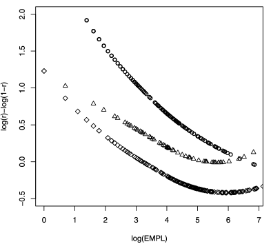
Figure 5: The logit function $\operatorname{logit}(p(x))=\log(p(x))-\log(1-p(x))$ for the smoothed response rates $r$ by the $\log$ transformed establishment size. This is displayed for establishments in the professional and business services industry category located in an MSA with over a million people. The circles represent the log-odds ratio by log size for establishments with $\mathit{MULTI}=1,$ the triangles are establishments with $\mathit{MULTI}=2,$ and the diamonds are establishments with $\mathit{MULTI}\geq 3.$ The response rate by transformed establishment size is estimated by a loess smoother.

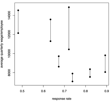
Figure 6: For the seven categories of mail survey-collected establishments defined by the regression tree model, the average wage is plotted by response rate. The average wage per employee is given for responding establishments (bottom) and nonresponding establishments (top). The line between the two estimates gives a visual representation of the difference between responding and nonresponding establishments within each category. All wage estimates are for the second quarter of 2005 and are produced from the QCEW records.

The fact that the differences in average wage per employee between respondents and nonresponders persist across categories, even among centrally collected units, gives cause for concern that the nonresponse bias could be nonignorable. If so, adjusting for nonresponse using the administrative wage data as well as the establishment characteristics may help to reduce nonresponse bias. Research on whether nonignorable nonresponse is a serious threat to the OES wage data, as well as potential adjustment, is currently underway.

The study findings are strong and have many possible implications for the OES survey program. Nonresponse has distinct patterns in the OES, based on employment size, industry, multi-establishment status, and metropolitan location. The OES program may want to consider survey design changes, such as focused contact or nonresponse follow-up for establishment groups with low response propensity and high wage differentials. These types of changes could be integrated into a responsive design, which OES is well set up to implement, given its multiple mailings. In addition, exploration of the QCEW average wage as an auxiliary variable in nonresponse bias adjustments may be a promising option.

OES may consider collecting more data via the central-collection mode as a way to improve response rates in multi-establishment firms. However, there are reasons for caution. First, establishment respondents have made a special request to provide data via a central collection arrangement. Given the respondent self-selection involved, it is unclear whether central collection could be implemented on a larger scale. Second, because of the relatively large difference in wages for responding and nonresponding centrally collected establishments, changing to this mode of collection is likely to have a small impact on bias reduction if this difference persists after the change. Before attempting to expand this type of collection, a serious assessment of how to reduce nonresponse among large firms reporting by this mode would need to be undertaken, as well as a test of the viability of the data collection mode for other multi-establishment firms.

Appendix: Simulations to compare regression tree and logistic regression modeling procedures

In this section we compare the performance of the regression tree modeling to the more common logistic regression. Specifically, we compare the nonparametric regression tree model to a parametric model obtained using stepwise logistic regression in R.

To compare the two approaches, we consider the accuracy of a given modeling procedure for predicting an establishment’s response propensity when the response propensity $p(\mathbf{x})$ is a function of the given values $\mathbf{x}.$ We test the two methods on five different functions for $p.$ For all five models we used randomly generated data containing six independent variables $\mathbf{x}=(x_{1},x_{2},x_{3},x_{4},c_{1},c_{2}).$ Four variables, $x_{1}$, $x_{2}$, $x_{3}$, and $x_{4},$ are integers uniformly distributed between 0 and 100 and two variables, $c1$ and $c2$, are categorical variables. The variable $c1$ has a binomial distribution with $n=4$ and $p=0.2$ and $c_{2}$ is Bernoulli with $p=0.3.$ The random variable $\mathbf{R}_{i}=(R_{i1},R_{i2},R_{i3},R_{i4},R_{i5})$ was then generated as independent Bernoulli random variables with $p=p(\mathbf{x})$ using the five models for $p(\mathbf{x})$ described below. Each generated data set had one hundred randomly generated points $(\mathbf{R}_{i},\mathbf{x}_{i})$ using the above distribution.

The first of the five models for $p(\mathbf{x})$ used to compare modeling procedures was the simple logistic model with no interactions

$$p_{1}(\mathbf{x})=\bigl{(}1+\exp\{-0.003(1+3x_{1}-2x_{2}+3x_{3})\}\bigr{)}^{-1}.$$

The second model was also a logistic model with one quadratic term and interactions among the variables. The logistic model used was

$$p_{2}(\mathbf{x})=\bigl{(}1+\exp\{-0.0001(x_{1}+2x_{2}-3x_{3}-x_{1}x_{2}+2x_{1}x_{3}+x_{3}^{2})\}\bigr{)}^{-1}.$$

The third model

$$p_{3}(\mathbf{x})=\bigl{(}1+\exp\{-0.0001(c_{1}x_{2}x_{3}-x_{1}x_{2}+2x_{1}x_{3}+c_{2}x_{3}^{2})\}\bigr{)}^{-1}$$

is logistic with higher order interactions among the variables. The fourth is the simple logistic model

$$p_{4}(\mathbf{x})=\bigl{(}1+\exp\{-0.01(x_{1}-x_{2})\}\bigr{)}^{-1}$$

for values of $\mathbf{x}$ with $x_{1}>35$ and with

$$p_{4}(\mathbf{x})=\bigl{(}1+\exp\{-0.01(2x_{1}+x_{2})\}\bigr{)}^{-1}$$

otherwise. The fifth modeled $p(\mathbf{x})$ using the tree model

For each simulated data set, we estimate the logistic model $\hat{p}_{L}$ and the regression tree model $\hat{p}_{T},$ for the response propensity for each of the five models of $p(x).$ A summary of the values of $p(\mathbf{x})$ produced by the five models is given in Table 6. Then for each model, we compare the predicted values $\hat{p}_{L}(\mathbf{x})$ and $\hat{p}_{T}(\mathbf{x})$ to the true model $p(\mathbf{x}).$ For the five models, using 100 data sets of $n=500,$ boxplots of the differences $\hat{p}_{L}(\mathbf{x})-p(\mathbf{x})$ and $\hat{p}_{T}(\mathbf{x})-p(\mathbf{x})$ are given for each quantile of $p(\mathbf{x})$ in Figure 7.

Table 6: Summary of values for $p(\mathbf{x})$, for the five models used in the simulation

Model	Min.	1st Qu.	Median	Mean	3rd Qu.	Max.
1	0.36	0.58	0.65	0.64	0.71	0.86
2	0.28	0.52	0.61	0.63	0.73	0.95
3	0.27	0.48	0.53	0.55	0.61	0.97
4	0.35	0.52	0.60	0.60	0.68	0.85
5	0.21	0.51	0.65	0.65	0.90	0.90

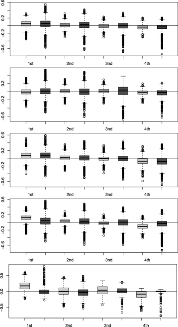
Figure 7: Boxplots of the differences between the true value of $p(\mathbf{x})$ and the predicted value for the log-linear model (light gray) and the tree predictor (dark gray) for each of the four quartiles of $p(\mathbf{x}).$ The whiskers are drawn at the most extreme data points that are within 1.5 times the inter-quartile range. Outliers are defined as any point beyond the whiskers and are drawn on the graph as circles. The black horizontal line was drawn at zero to help see the skewness of the errors for the different estimators.

The results show that both methods of modeling worked reasonably well on all the data sets. The logistic modeling performed slightly better when $p(\mathbf{x})$ fit a log linear model but worse than the tree model, as the $p(\mathbf{x})$ had discontinuities. When using stepwise regression to find the best logistic model, we searched over all models using the six variables, one-way interactions, and quadratic terms. Note that this was sufficient to fit model 1 and model 2 perfectly. This would not be known in practice, and it is not clear how to choose the number of interactions to include. When too many interactions were included in the possible models, the procedure performed less efficiently.

Acknowledgments

The views expressed on statistical, methodological, technical, and operational issues are those of the authors and not necessarily those of the U.S. Bureau of Labor Statistics. The authors thank the Editors and referees for their helpful comments, as well as John L. Eltinge and Jean Opsomer for comments and discussions that improved this article.

References

- Breiman et al. (1984) {bbook}[mr] \bauthor\bsnmBreiman, \bfnmLeo\binitsL., \bauthor\bsnmFriedman, \bfnmJerome H.\binitsJ. H., \bauthor\bsnmOlshen, \bfnmRichard A.\binitsR. A. and \bauthor\bsnmStone, \bfnmCharles J.\binitsC. J. (\byear1984). \btitleClassification and Regression Trees. \bpublisherWadsworth Advanced Books and Software, \baddressBelmont, CA. \bidmr=0726392 \bptokimsref \endbibitem
- Eltinge and Yansaneh (1997) {barticle}[auto:STB—2012/01/18—07:48:53] \bauthor\bsnmEltinge, \bfnmJ.\binitsJ. and \bauthor\bsnmYansaneh, \bfnmI.\binitsI. (\byear1997). \btitleDiagnostics for formation of nonresponse adjustment cells, with an application to income nonresponse in the U.S. Consumer Expenditure Survey. \bjournalSurvey Methodology \bvolume23 \bpages33–40. \bptokimsref \endbibitem
- Göksel, Judkins and Mosher (1992) {barticle}[auto:STB—2012/01/18—07:48:53] \bauthor\bsnmGöksel, \bfnmH.\binitsH., \bauthor\bsnmJudkins, \bfnmD.\binitsD. and \bauthor\bsnmMosher, \bfnmW.\binitsW. (\byear1992). \btitleNonresponse adjustment for a telephone follow-up to a national in-person survey. \bjournalJournal of Official Statistics \bvolume8 \bpages417–431. \bptokimsref \endbibitem
- Gordon and Olshen (1978) {barticle}[mr] \bauthor\bsnmGordon, \bfnmLouis\binitsL. and \bauthor\bsnmOlshen, \bfnmRichard A.\binitsR. A. (\byear1978). \btitleAsymptotically efficient solutions to the classification problem. \bjournalAnn. Statist. \bvolume6 \bpages515–533. \bidissn=0090-5364, mr=0468035 \bptokimsref \endbibitem
- Gordon and Olshen (1980) {barticle}[mr] \bauthor\bsnmGordon, \bfnmLouis\binitsL. and \bauthor\bsnmOlshen, \bfnmRichard A.\binitsR. A. (\byear1980). \btitleConsistent nonparametric regression from recursive partitioning schemes. \bjournalJ. Multivariate Anal. \bvolume10 \bpages611–627. \biddoi=10.1016/0047-259X(80)90074-3, issn=0047-259X, mr=0599694 \bptokimsref \endbibitem
- Hastie, Tibshirani and Friedman (2001) {bbook}[mr] \bauthor\bsnmHastie, \bfnmTrevor\binitsT., \bauthor\bsnmTibshirani, \bfnmRobert\binitsR. and \bauthor\bsnmFriedman, \bfnmJerome\binitsJ. (\byear2001). \btitleThe Elements of Statistical Learning: Data Mining, Inference, and Prediction. \bpublisherSpringer, \baddressNew York. \bidmr=1851606 \bptokimsref \endbibitem
- Kim and Kim (2007) {barticle}[mr] \bauthor\bsnmKim, \bfnmJae Kwang\binitsJ. K. and \bauthor\bsnmKim, \bfnmJay J.\binitsJ. J. (\byear2007). \btitleNonresponse weighting adjustment using estimated response probability. \bjournalCanad. J. Statist. \bvolume35 \bpages501–514. \biddoi=10.1002/cjs.5550350403, issn=0319-5724, mr=2381396 \bptokimsref \endbibitem
- Kott and Chang (2010) {barticle}[mr] \bauthor\bsnmKott, \bfnmPhillip S.\binitsP. S. and \bauthor\bsnmChang, \bfnmTed\binitsT. (\byear2010). \btitleUsing calibration weighting to adjust for nonignorable unit nonresponse. \bjournalJ. Amer. Statist. Assoc. \bvolume105 \bpages1265–1275. \biddoi=10.1198/jasa.2010.tm09016, issn=0162-1459, mr=2752620 \bptokimsref \endbibitem
- LeBlanc and Tibshirani (1998) {barticle}[auto:STB—2012/01/18—07:48:53] \bauthor\bsnmLeBlanc, \bfnmM.\binitsM. and \bauthor\bsnmTibshirani, \bfnmR.\binitsR. (\byear1998). \btitleMonotone shrinkage of trees. \bjournalJ. Comput. Graph. Statist. \bvolume7 \bpages417–433. \bptokimsref \endbibitem
- Little (1982) {barticle}[mr] \bauthor\bsnmLittle, \bfnmRoderick J. A.\binitsR. J. A. (\byear1982). \btitleModels for nonresponse in sample surveys. \bjournalJ. Amer. Statist. Assoc. \bvolume77 \bpages237–250. \bidissn=0162-1459, mr=0664675 \bptokimsref \endbibitem
- Little (1986) {barticle}[auto:STB—2012/01/18—07:48:53] \bauthor\bsnmLittle, \bfnmR.\binitsR. (\byear1986). \btitleSurvey nonresponse adjustments for estimates of means. \bjournalInternational Statistical Review \bvolume2 \bpages139–157. \bptokimsref \endbibitem
- Little and Vartivarian (2005) {barticle}[auto:STB—2012/01/18—07:48:53] \bauthor\bsnmLittle, \bfnmR.\binitsR. and \bauthor\bsnmVartivarian, \bfnmS.\binitsS. (\byear2005). \btitleDoes weighting for nonresponse increase the variance of survey means? \bjournalSurvey Methodology \bvolume31 \bpages161–168. \bptokimsref \endbibitem
- Opsomer and Miller (2005) {barticle}[mr] \bauthor\bsnmOpsomer, \bfnmJ. D.\binitsJ. D. and \bauthor\bsnmMiller, \bfnmC. P.\binitsC. P. (\byear2005). \btitleSelecting the amount of smoothing in nonparametric regression estimation for complex surveys. \bjournalJ. Nonparametr. Stat. \bvolume17 \bpages593–611. \biddoi=10.1080/10485250500054642, issn=1048-5252, mr=2141364 \bptokimsref \endbibitem
- Petroni et al. (2004) {bmisc}[auto:STB—2012/01/18—07:48:53] \bauthor\bsnmPetroni, \bfnmR.\binitsR., \bauthor\bsnmSigman, \bfnmR.\binitsR., \bauthor\bsnmWillimack, \bfnmD.\binitsD., \bauthor\bsnmCohen, \bfnmS.\binitsS. and \bauthor\bsnmTucker, \bfnmC.\binitsC. (\byear2004). \bhowpublishedResponse rates and nonresponse in establishment surveys–BLS and Census Bureau. In Federal Economic Statistics Advisory Committee Meeting (December). Available at http:// www.bea.gov/about/pdf/ResponseratesnonresponseinestablishmentsurveysFESAC121404. pdf. \bptokimsref \endbibitem
- Phipps and Jones (2007) {bmisc}[auto:STB—2012/01/18—07:48:53] \bauthor\bsnmPhipps, \bfnmP.\binitsP. and \bauthor\bsnmJones, \bfnmC.\binitsC. (\byear2007). \bhowpublishedFactors affecting response to the occupational employment statistics survey. In Proceedings of the 2007 Federal Committee on Statistical Methodology Research Conference. Available at http://www.fcsm.gov/07papers/ Phipps.II-A.pdf. \bptokimsref \endbibitem
- Rosenbaum and Rubin (1983) {barticle}[mr] \bauthor\bsnmRosenbaum, \bfnmPaul R.\binitsP. R. and \bauthor\bsnmRubin, \bfnmDonald B.\binitsD. B. (\byear1983). \btitleThe central role of the propensity score in observational studies for causal effects. \bjournalBiometrika \bvolume70 \bpages41–55. \biddoi=10.1093/biomet/70.1.41, issn=0006-3444, mr=0742974 \bptokimsref \endbibitem
- Schouten and de Nooij (2005) {bmisc}[auto:STB—2012/01/18—07:48:53] \bauthor\bsnmSchouten, \bfnmB.\binitsB. and \bauthor\bparticlede \bsnmNooij, \bfnmG.\binitsG. (\byear2005). \bhowpublishedNonresponse adjustment using classification trees. Discussion Paper 05001, Statistics Netherlands. Available at http://www.cbs. nl/NR/rdonlyres/1245916E-80D5-40EB-B047-CC45E728B2A3/0/200501x10pub.pdf. \bptokimsref \endbibitem
- Shao (1993) {barticle}[mr] \bauthor\bsnmShao, \bfnmJun\binitsJ. (\byear1993). \btitleLinear model selection by cross-validation. \bjournalJ. Amer. Statist. Assoc. \bvolume88 \bpages486–494. \bidissn=0162-1459, mr=1224373 \bptokimsref \endbibitem
- Tomaskovic-Devey, Leiter and Thompson (1994) {barticle}[auto:STB—2012/01/18—07:48:53] \bauthor\bsnmTomaskovic-Devey, \bfnmD.\binitsD., \bauthor\bsnmLeiter, \bfnmJ.\binitsJ. and \bauthor\bsnmThompson, \bfnmS.\binitsS. (\byear1994). \btitleOrganizational survey nonresponse. \bjournalAdministrative Science Quarterly \bvolume39 \bpages439–457. \bptokimsref \endbibitem
- Toth and Eltinge (2011) {barticle}[auto:STB—2012/01/18—07:48:53] \bauthor\bsnmToth, \bfnmD.\binitsD. and \bauthor\bsnmEltinge, \bfnmJ.\binitsJ. (\byear2011). \btitleBuilding consistent regression trees from complex sample data. \bjournalJ. Amer. Statist. Assoc. \bvolume106 \bpages1626–1636. \bptokimsref \endbibitem
- Toth and Eltinge (2008) {bmisc}[auto:STB—2012/01/18—07:48:53] \bauthor\bsnmToth, \bfnmD.\binitsD. and \bauthor\bsnmEltinge, \bfnmJ.\binitsJ. (\byear2008). \bhowpublishedSimple function representation of regression trees. Bureau of Labor Statistics Technical Report. \bptokimsref \endbibitem
- Vartivarian and Little (2002) {bmisc}[auto:STB—2012/01/18—07:48:53] \bauthor\bsnmVartivarian, \bfnmS.\binitsS. and \bauthor\bsnmLittle, \bfnmR.\binitsR. (\byear2002). \bhowpublishedOn the formation of weighting adjustment cells for unit nonresponse. In Proceedings of the Survey Research Methods Section 3553–3558. Amer. Statist. Assoc., Alexandria, VA. \bptokimsref \endbibitem