Estimation and testing for spatially indexed curves with application to ionospheric and magnetic field trends

Abstract

We develop methodology for the estimation of the functional mean and the functional principal components when the functions form a spatial process. The data consist of curves $X(\mathbf{s}_{k};t),t\in[0,T],$ observed at spatial locations $\mathbf{s}_{1},\mathbf{s}_{2},\ldots,\mathbf{s}_{N}$. We propose several methods, and evaluate them by means of a simulation study. Next, we develop a significance test for the correlation of two such functional spatial fields. After validating the finite sample performance of this test by means of a simulation study, we apply it to determine if there is correlation between long-term trends in the so-called critical ionospheric frequency and decadal changes in the direction of the internal magnetic field of the Earth. The test provides conclusive evidence for correlation, thus solving a long-standing space physics conjecture. This conclusion is not apparent if the spatial dependence of the curves is neglected.

T1Supported in part by NSF Grants DMS-08-04165 and DMS-09-31948.

, , and

1 Introduction

The contribution of this paper to statistics is two-fold: (1) we develop estimation methodology for the functional mean and the functional principal components (FPCs) when the functions form a spatial field; (2) we propose a significance test to determine if two families of curves observed at the same spatial locations are uncorrelated. The contribution to space physics consists in solving a controversy regarding the impact of long-term changes in the internal magnetic field of the Earth on long-term ionospheric trends. The required physics background is provided later in this section, and in Section 8.

The data is modeled as curves $X(\mathbf{s}_{k};t),t\in[0,T],$ observed at spatial locations $\mathbf{s}_{1},\mathbf{s}_{2},\ldots,\mathbf{s}_{N}$. Such functional data structures are quite common, but typically the spatial dependence and the spatial distribution of the points $\mathbf{s}_{k}$ are not taken into account. A fundamental question is how to estimate the mean function of curves indexed by spatial locations. Clearly, curves located at close-by points look similar and must be given smaller weights than curves at points far apart. In addition to the mean function, FPCs play a fundamental role in functional data analysis. Good estimators of FPCs are needed to construct reliable testing and classification procedures, but such issues have been addressed only in the contexts of independent curves, with focus on sparsity and measurement error. The geophysical data that motivate this research are available at fine temporal grids and are measured with errors that are negligible relative to the objectives of the statistical analysis. A focus of recent geophysical research is on the detection and estimation of global and/or regional long-term trends (the global warming paradigm), so before a statistical analysis is undertaken, the data are typically smoothed to remove daily or even annual periodicity. The question we address is how to combine the temporal trajectories available at many spatial locations to obtain meaningful summary trends. We argue that one can do better than using simple averaging. The focus of this paper is thus on combining information from spatially dependent curves, which are smooth and available at all time points.

Figure 1: F2-layer critical frequency curves at three locations. Top to bottom (latitude in parentheses): Yakutsk (62.0), Yamagawa (31.2), Manila (14.7). The functions exhibit a latitudinal trend in amplitude.

Figure 2: Locations of 218 ionosonde stations. Circles represent the 32 stations with the longest complete records.

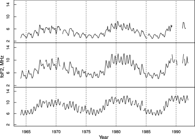
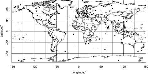
Many environmental and geophysical data sets fall into the framework considered in this paper. The data set that motivated this research consists of the curves of the ionospheric F2-layer critical frequency, foF2. Three such curves are shown in Figure 1. In principle, foF2 curves are available at over 200 locations throughout the globe (see Figure 2), but sufficiently complete data are available at only 30–40 locations which are very unevenly spread; for example, there is a dense network of observatories over Europe and practically no data over the oceans. The study of this data set has been motivated by the hypothesis of Roble and Dickinson (1989), who suggested that the increasing amounts of (radiative) greenhouse gases should lead to global cooling in mesosphere and thermosphere, as opposed to the global warming in lower troposphere; cf. Figure 3. Rishbeth (1990) pointed out that such cooling would result in a thermal contraction and the global lowering of the ionospheric peak densities, which can be computed from the critical frequency foF2. The last twenty years have seen very extensive research in this area; see Laštovička et al. (2008) for a partial overview. One of the difficulties in determining a global trend is that the foF2 curves appear to exhibit trends in opposing directions over various regions. A possible explanation suggests that these trends are caused by long-term trends in the magnetic field of the Earth. There is, however, currently not agreement in the space physics community if this is indeed the case. In general, to make any trends believable, a suitable statistical modeling and a proper treatment of “errors and uncertainties” is called for [Ulich, Clilverd and Rishbeth (2003)]. This paper makes a contribution in this direction. Space physics data measured at terrestrial observatories always come in the form of temporal curves at fixed spatial locations. In Maslova et al. (2009), Maslova et al. (2010a) and Maslova et al. (2010b) the tools of functional data analysis were used to study such data, but the spatial dependence of the curves was not fully exploited.

Figure 3: Typical profile of day time ionosphere. The curve shows electron density as a function of height. The right vertical axis indicates the D, E and F regions.

Spatio-temporal modeling has received a great deal of attention of late; see Part V of Gelfand et al. (2010) and Chapters 3, 4 and 6 of Finkenstaedt, Held and Isham (2007) which discuss spatio-temporal models for geostatistical data. There has, however, not been much research specifically on spatially indexed functional data; Delicado et al. (2010) review recent contributions. For geostatistical functional data, several approaches to kriging have been proposed; see Yamanishi and Tanaka (2003), Nerini, Monestiez and Manté (2010), Giraldo, Delicado and Mateu (2011a) and Bel et al. (2011).

Throughout the paper, $\{X(\mathbf{s})\}$ denotes a random field defined on a spatial domain and taking values in the Hilbert space $L^{2}=L^{2}([0,1])$ with the inner product

$$\langle f,g\rangle=\int_{0}^{1}f(t)g(t)\,dt,\qquad f,g\in L^{2}.$$

The value of the function $X(\mathbf{s})\in L^{2}$ at time $t\in[0,1]$ is denoted by $X(\mathbf{s};t)$. We postulate the model

$$X(\mathbf{s};t)=\mu(t)+\sum_{i=1}^{\infty}\xi_{i}(\mathbf{s})e_{i}(t),\qquad\xi_{i}(\mathbf{s})=\langle X(\mathbf{s})-\mu,e_{i}\rangle,$$ (1)

where the $e_{i}$ form a complete orthonormal system. Note that the mean function $\mu$ and the FPCs $e_{i}$ do not depend on $\mathbf{s}$. A sufficient condition for this is that the distribution in $L^{2}$ of the function $X(\mathbf{s})$ does not depend on the location $\mathbf{s}$. A stronger sufficient condition is the strict stationarity of the field $\{X(\mathbf{s})\}$.

For the applications we have in mind, it is enough to assume that the spatial domain is a subset of the plane or a two-dimensional sphere. On the plane, the distance between points is the usual Euclidean distance; on the sphere, we use the chordal distance defined as the Euclidean distance in the three-dimensional space. The reason for using the chordal distance is that any spatial covariance functions in $\mathbb{R}^{3}$ restricted to the unit sphere is then also a covariance function on the sphere. Denoting the latitude by $L$ and the longitude by $l$, the chordal distance, $0\leq d_{k,\ell}\leq 2$, between two points, $\mathbf{s}_{k},\mathbf{s}_{\ell}$, on the unit sphere is given by

$$\qquad d_{k,\ell}=2\biggl{[}\sin^{2}\biggl{(}\frac{L_{k}-L_{\ell}}{2}\biggr{)}+\cos{L_{k}}\cos{L_{\ell}}\sin^{2}\biggl{(}\frac{l_{k}-l_{\ell}}{2}\biggr{)}\biggr{]}^{1/2}.$$ (2)

For arbitrary (not necessarily spatially indexed) functions, $X_{1},X_{2},\ldots,X_{N}$, the sample mean is defined as $\bar{X}_{N}=N^{-1}\sum_{n=1}^{N}X_{n},$ and the sample covariance operator as

$$\widehat{C}(x)=N^{-1}\sum_{n=1}^{N}[\langle(X_{n}-\bar{X}_{N}),x\rangle(X_{n}-\bar{X}_{N})],\qquad x\in L^{2}.$$

The sample FPCs are computed as the eigenfunctions of $\widehat{C}$. These are the estimates produced by several software packages, including the popular R package fda; see Ramsay, Hooker and Graves (2009). The consistency of the sample mean and the sample FPCs relies on the assumption that the functional observations form a simple random sample. If the functions $X_{k}=X(\mathbf{s}_{k})$ are spatially distributed, the sample mean and the sample FPCs need not even be consistent; see Hörman and Kokoszka (2012). This happens if the spatial dependence is strong or if there are clusters of the points $\mathbf{s}_{k}$. We will demonstrate that better estimators are available and we will use them as part of the procedure for testing the independence of two functional fields $\{X(\mathbf{s}),\mathbf{s}\in\mathbf{S}\}$ and $\{Y(\mathbf{s}),\mathbf{s}\in\mathbf{S}\}$. The procedure is based on the observed pairs of functions $(X(\mathbf{s}_{k}),Y(\mathbf{s}_{k})),1\leq k\leq N$. The test we propose is applied to ionosonde (X) and magnetic (Y) curves, and conclusively shows that the temporal evolution of these two families is strongly correlated.

The remainder of the paper is organized as follows. Sections 2 and 3 focus, respectively, on the estimation of the mean function and the FPCs in a spatial setting. Section 4 demonstrates by means of a simulation study that the methods we propose improve on the standard approach, and discusses their relative performance and computational cost. In Section 5 we develop a test for the correlation of two functional spatial fields. This test requires estimation of a covariance tensor. After addressing this issue in Section 6, we study in Section 7 the finite sample properties of several implementations of the test. Finally, in Section 8 we apply the methodology developed in the previous section to test for the correlation between the ionospheric critical frequency and magnetic curves.

2 Estimation of the mean function

We propose three methods of estimating the mean function $\mu$, which we call M1, M2, M3. As will become apparent in this section, several further variants, not discussed here, are conceivable. But the results of Section 4 show that while all these methods offer an improvement over the simple sample mean, their performance is comparable. We represent the observed functions as

$$X(\mathbf{s}_{k};t)=\mu(t)+{\varepsilon}(\mathbf{s}_{k};t),\qquad k=1,2,\ldots,N,$$ (3)

where ${\varepsilon}$ is an unobservable field with $E{\varepsilon}(\mathbf{s};t)=0$. All methods assume that the function valued field ${\varepsilon}(\cdot)$ is strictly stationary and isotropic, even though weaker, more technical assumptions could be made for the specific methods. Methods M1 and M2 are akin to the kriging technique advocated by Giraldo, Delicado and Mateu (2011a) in that they treat the curves as single entities and seek to minimize the integrated mean squared error. Method M3 is similar in spirit to the approach to functional kriging developed by Nerini, Monestiez and Manté (2010) and Giraldo, Delicado and Mateu (2011b) who use cokriging of basis coefficients.

Methods M1 and M2 estimate $\mu$ by the weighted average

$$\hat{\mu}_{N}=\sum_{n=1}^{N}w_{n}X(\mathbf{s}_{n}).$$ (4)

The optimal weights $w_{k}$ are defined to minimize $E\|\sum_{n=1}^{N}w_{n}X(\mathbf{s}_{n})-\mu\|^{2}$ subject to the condition $\sum_{n=1}^{N}w_{n}=1$ ($\|x\|^{2}=\int_{0}^{1}x^{2}(t)\,dt$). Using the method of the Lagrange multiplier, we see that the unknowns $w_{1},w_{2},\ldots,w_{N},r$ are solutions to the system of $N+1$ equations

$$\sum_{n=1}^{N}w_{n}=1,\qquad\sum_{k=1}^{N}w_{k}C_{kn}-r=0,\qquad n=1,2,\ldots,N,$$ (5)

where

$$C_{k\ell}=E[\langle{\varepsilon}(\mathbf{s}_{k}),{\varepsilon}(\mathbf{s}_{\ell})\rangle].$$ (6)

Set $\mathbf{w}=(w_{1},\ldots,w_{N})^{T}$. An easy way to solve the equations in (5) is to compute $\mathbf{v}=\mathbf{C}^{-1}{\mathbf{1}}$, where $\mathbf{C}=[C_{k\ell},1\leq k,\ell\leq N]$, and then set $\mathbf{w}=a\mathbf{v}$, where $a$ is a constant such that ${\mathbf{1}}^{T}\mathbf{w}=1$.

Method M1. At each time point $t_{j}$, we fit a parametric spatial model to the scalar field $X(\mathbf{s};t_{j})$. To focus attention, we provide formulas for the exponential model

$${\operatorname{Cov}}(X(\mathbf{s}_{k};t_{j}),X(\mathbf{s}_{\ell};t_{j}))={\sigma}^{2}(t_{j})\exp\biggl{\{}-\frac{d(\mathbf{s}_{k},\mathbf{s}_{\ell})}{\rho(t_{j})}\biggr{\}}.$$ (7)

It is clear how they can be modified for other popular models.

Observe that under model (7),

$$C_{k\ell} = E\int\bigl{(}X(\mathbf{s}_{k};t)-\mu(t)\bigr{)}\bigl{(}X(\mathbf{s}_{\ell};t)-\mu(t)\bigr{)}\,dt$$

$$= \int{\operatorname{Cov}}(X(\mathbf{s}_{k};t_{j}),X(\mathbf{s}_{\ell};t_{j}))\,dt$$

$$= \int{\sigma}^{2}(t)\exp\biggl{\{}-\frac{d(\mathbf{s}_{k},\mathbf{s}_{\ell})}{\rho(t)}\biggr{\}}\,dt.$$

One way to estimate $C_{k\ell}$ is to set

$$\widehat{C}_{k\ell}=\int\hat{\sigma}^{2}(t)\exp\biggl{\{}-\frac{d(\mathbf{s}_{k},\mathbf{s}_{\ell})}{\hat{\rho}(t)}\biggr{\}}\,dt,$$ (8)

with the estimates $\hat{\sigma}^{2}(t_{j})$ and $\hat{\rho}(t_{j})$ obtained using some version of empirical variogram, (29) or (30) in this study.

Another way to proceed is to replace the $\hat{\rho}(t_{j})$ by their average $\hat{\rho}=m^{-1}\*\sum_{j=1}^{m}\hat{\rho}(t_{j}),$ where $m$ is the count of the $t_{j}$ at which the variogram is estimated successfully. Then, the $C_{k\ell}$ are approximated by

$$\widehat{C}_{k\ell}=\biggl{(}\int\hat{\sigma}^{2}(t)\,dt\biggr{)}\exp\biggl{\{}-\frac{d(\mathbf{s}_{k},\mathbf{s}_{\ell})}{\hat{\rho}}\biggr{\}}.$$

As explained above, in order to compute the weights $w_{j}$ in (5), it is enough to know the matrix $\mathbf{C}$ only up to a multiplicative constant. Thus, we may set

$$\widehat{C}_{k\ell}=\exp\biggl{\{}-\frac{d(\mathbf{s}_{k},\mathbf{s}_{\ell})}{\hat{\rho}}\biggr{\}}.$$ (9)

Once the matrix $\mathbf{C}$ has been estimated, we compute the weights $w_{j}$, and estimate the mean via (4).

If (8) is used, we refer to this method as M1a; if (9) is used, we call it M1b.

Method M1 relies on the estimation of the variograms at every point $t_{j}$. Method M2, described below, requires only one optimization, so it is much faster than M1.

Method M2. We define the functional variogram

$$2\gamma(\mathbf{s}_{k},\mathbf{s}_{\ell}) = E\|X(\mathbf{s}_{k})-X(\mathbf{s}_{\ell})\|^{2}$$

$$= 2E\|X(\mathbf{s}_{k})-\mu\|^{2}-2E[\langle X(\mathbf{s}_{k})-\mu,X(\mathbf{s}_{\ell})-\mu\rangle]$$

$$= 2E\|X(\mathbf{s})-\mu\|^{2}-2C_{k\ell}.$$

The variogram (2) can be estimated by its empirical counterparts, like (29) or (30), with the $|X(\mathbf{s}_{k})-X(\mathbf{s}_{\ell})|$ replaced by

$$\|X(\mathbf{s}_{k})-X(\mathbf{s}_{\ell})\|=\biggl{\{}\int\bigl{(}X(\mathbf{s}_{k};t)-X(\mathbf{s}_{\ell};t)\bigr{)}^{2}\,dt\biggr{\}}^{1/2}.$$

Next, we fit a parametric model, for example, we postulate that

$$\gamma(\mathbf{s}_{k},\mathbf{s}_{\ell})={\sigma}_{f}^{2}\biggl{(}1-\exp\biggl{\{}-\frac{d(\mathbf{s}_{k},\mathbf{s}_{\ell})}{\rho_{f}}\biggr{\}}\biggr{)}.$$ (11)

The subscript $f$ is used to emphasize the functional variogram. Denoting by $\hat{\rho}_{f}$ the resulting NLS estimate, we estimate the $C_{kl}$ by (9) with $\hat{\rho}$ replaced by $\hat{\rho}_{f}$.

Method M3. This method uses a basis expansion of the functional data, it does not use the weighted sum (4). Suppose $B_{j},1\leq j\leq K,$ are elements of a functional basis with $K$ so large that for each $k$

$$X(\mathbf{s}_{k})\approx\sum_{j\leq K}\langle B_{j},X(\mathbf{s}_{k})\rangle B_{j}$$ (12)

to a good approximation. By (3), we obtain for every $j$

$$\langle B_{j},X(\mathbf{s}_{k})\rangle=\langle B_{j},\mu\rangle+\langle B_{j},{\varepsilon}(\mathbf{s}_{k})\rangle,\qquad k=1,2,\ldots,N.$$ (13)

For every fixed $j$, the $\langle B_{j},X(\mathbf{s}_{k})\rangle$ form a stationary and isotropic scalar spatial field with a constant unknown mean $\langle B_{j},\mu\rangle$. This mean can be estimated by postulating a covariance structure for each $\langle B_{j},X(\mathbf{s}_{k})\rangle$, for example,

$${\operatorname{Cov}}(\langle B_{j},X(\mathbf{s}_{k})\rangle,\langle B_{j},X(\mathbf{s}_{\ell})\rangle)={\sigma}_{j}^{2}\exp\biggl{\{}-\frac{d(\mathbf{s}_{k},\mathbf{s}_{\ell})}{\rho_{j}}\biggr{\}}.$$

The mean $\langle B_{j},\mu\rangle$ is estimated by a weighted average of the $\langle B_{j},X(\mathbf{s}_{k})\rangle$ (the weights depend on $j$). Denote the resulting estimate by $\hat{\mu}_{j}$. The mean function $\mu$ is then estimated by $\hat{\mu}(t)=\sum_{j\leq K}\hat{\mu}_{j}B_{j}(t)$.

3 Estimation of the principal components

Assume now that the mean function $\mu$ has been estimated, and this estimate is subtracted from the data. To simplify the formulas, in the following we thus assume that $EX(\mathbf{s})=0$.

We consider analogs of methods M2 and M3. Extending Method M1 is possible, but presents a computational challenge because a parametric spatial model would need to be estimated for every pair $(t_{i},t_{j})$. For the ionosonde data studied in Section 8, there are 336 points $t_{j}$. Estimation on a single data set would be feasible, but not a simulation study based on thousands of replications.

In both approaches, which we term CM2 and CM3, the FPCs are estimated by expansions of the form

$$v_{j}(t)=\sum_{{\alpha}=1}^{K}x_{\alpha}^{(j)}B_{\alpha}(t),$$ (14)

where the $B_{\alpha}$ are elements of an orthonormal basis. We first describe an analog of method M3, which is conceptually and computationally simpler.

Method CM3. The starting point is the expansion

$$X(\mathbf{s};t)=\sum_{j=1}^{\infty}\xi_{j}(\mathbf{s})B_{j}(t),$$

where, by the orthonormality of the $B_{j}$, the $\xi_{j}(\mathbf{s})$ form an observable field $\xi_{j}(\mathbf{s}_{k})=\langle B_{j},X(\mathbf{s}_{k})\rangle$. Using the orthonormality of the $B_{j}$ again, we obtain

$$C(B_{j}) = E\Biggl{[}\Biggl{\langle}\sum_{{\alpha}=1}^{\infty}\xi_{\alpha}(\mathbf{s})B_{\alpha},B_{j}\Biggr{\rangle}\sum_{i=1}^{\infty}\xi_{i}(\mathbf{s})B_{i}\Biggr{]}$$

$$= E\Biggl{[}\xi_{j}(\mathbf{s})\sum_{i=1}^{\infty}\xi_{i}(\mathbf{s})B_{i}\Biggr{]}$$

$$= \sum_{i=1}^{\infty}E[\xi_{i}(\mathbf{s})\xi_{j}(\mathbf{s})]B_{i}.$$

Thus, to estimate $C$, we must estimate the means $E[\xi_{i}(\mathbf{s})\xi_{j}(\mathbf{s})]$.

Fix $i$ and $j$, and define the scalar field $z$ by $z(\mathbf{s})=\xi_{i}(\mathbf{s})\xi_{j}(\mathbf{s}).$ We can postulate a parametric model for the covariance structure of the field $z(\cdot)$, and use an empirical variogram to estimate $\mu_{z}=Ez(\mathbf{s})$ as a weighted average of the $z(\mathbf{s}_{k})$. Denote the resulting estimate by $\hat{r}_{ij}$.

The empirical version of (3) is then

$$\widehat{C}(B_{j})=\sum_{i=1}^{K}\hat{r}_{ij}B_{i}.$$ (16)

Relation (16) defines the estimator $\widehat{C}$ which acts on the span of $B_{j}$, $1\leq j\leq K$.

Its eigenfunctions are of the form $x=\sum_{1\leq{\alpha}\leq K}x_{\alpha}B_{\alpha}$. Observe that

$$\widehat{C}(x)=\sum_{\alpha}x_{\alpha}\sum_{i}\hat{r}_{i{\alpha}}B_{i}=\sum_{i}\biggl{(}\sum_{\alpha}\hat{r}_{i{\alpha}}x_{\alpha}\biggr{)}B_{i}.$$

On the other hand,

$${\lambda}x=\sum_{i}{\lambda}x_{i}B_{i}.$$

Since the $B_{i}$ form an orthonormal basis, we obtain

$$\sum_{\alpha}\hat{r}_{i{\alpha}}x_{\alpha}={\lambda}x_{i}.$$

Setting

$$\mathbf{x}=[x_{1},x_{2},\ldots,x_{K}]^{T},\qquad\widehat{\mathbf{R}}=[\hat{r}_{ij},1\leq i,j\leq K],$$

we can write the above as a matrix equation

$$\widehat{\mathbf{R}}\mathbf{x}={\lambda}\mathbf{x}.$$ (17)

Denote the solutions to (17) by

$$\hat{\mathbf{x}}^{(j)}=\bigl{[}\hat{x}^{(j)}_{1},\hat{x}^{(j)}_{2},\ldots,\hat{x}^{(j)}_{k}\bigr{]}^{T},\qquad{\hat{\lambda}}_{j},\qquad 1\leq j\leq K.$$ (18)

The $\hat{\mathbf{x}}^{(j)}$ satisfy $\sum_{{\alpha}=1}^{K}\hat{x}^{(j)}_{\alpha}\hat{x}^{(i)}_{\alpha}={\delta}_{ij}$. Therefore, the ${\hat{v}}_{j}$ defined by

$${\hat{v}}_{j}=\sum_{{\alpha}=1}^{K}\hat{x}^{(j)}_{\alpha}B_{\alpha}$$ (19)

are also orthonormal (because the $B_{j}$ are orthonormal). The ${\hat{v}}_{j}$ given by (19) are the estimators of the FPCs, and the ${\hat{\lambda}}_{j}$ in (18) of the corresponding eigenvalues.

As in method M3, the value of $K$ can be taken to the number of basis functions used to create the functional objects in R, so it can be a relatively large number, for example, $K=49$. Even though the range of $j$ in (18) and (19) runs up to $K$, only the first few estimated FPCs ${\hat{v}}_{j}$ would be used in further work.

Method CM2. Recall that under the assumption of zero mean function, the covariance operator is defined by $C(x)=E[\langle X(\mathbf{s}),x\rangle X(\mathbf{s})].$ It can be estimated by the simple average

$$\frac{1}{N}\sum_{n=1}^{N}\langle X(\mathbf{s}_{n}),\cdot\rangle X(\mathbf{s}_{n})=\frac{1}{N}\sum_{n=1}^{N}C_{k},$$ (20)

where $C_{k}$ is the operator defined by

$$C_{k}(x)=\langle X(\mathbf{s}_{k}),x\rangle X(\mathbf{s}_{k}).$$

As for the mean, more precise estimates can be obtained by using the weighted average

$$\widehat{C}=\sum_{k=1}^{N}w_{k}C_{k}.$$ (21)

Before discussing the estimation of the weights $w_{k}$, we comment that the FPCs $v_{j}$ and their eigenvalues ${\lambda}_{j}$ can be estimated using (21) and the representation (14). As in method CM3, set $x=\sum_{1\leq{\alpha}\leq K}x_{\alpha}B_{\alpha}$, and observe that

$$\widehat{C}(x)=\sum_{j=1}^{K}\Biggl{(}\sum_{{\alpha}=1}^{K}s_{j{\alpha}}x_{\alpha}\Biggr{)}B_{j},$$

where

$$s_{j{\alpha}}=\sum_{k=1}^{N}w_{k}\langle X_{k},B_{j}\rangle\langle X_{k},B_{\alpha}\rangle.$$

Thus, analogously to (17), we obtain a matrix equation $\mathbf{S}\mathbf{x}={\lambda}\mathbf{x}$, from which the estimates of the $v_{j},{\lambda}_{j}$ can be found as in (18) and (19).

We now return to the estimation of the weights $w_{k}$ in (21). One way to define the optimal weights is to require that they minimize the expected Hilbert–Schmidt norm of $\widehat{C}-C$. Recall that the Hilbert–Schmidt norm of an operator $K$ is defined by

$$\|K\|_{{\mathcal{S}}}^{2}=\sum_{i=1}^{\infty}\|K(e_{i})\|^{2}=\sum_{i=1}^{\infty}\int|K(e_{i})(t)|^{2}\,dt,$$

where $\{e_{i},i\geq 1\}$ is any orthonormal basis in $L^{2}$. Since $\|\cdot\|_{{\mathcal{S}}}$ is a norm in the the Hilbert space ${\mathcal{S}}$ of the Hilbert–Schmidt operators with the inner product

$$\langle K_{1},K_{2}\rangle_{{\mathcal{S}}}=\sum_{i=1}^{\infty}\langle K_{1}(e_{i}),K_{2}(e_{i})\rangle,$$

we can repeat all algebraic manipulations needed to obtain the weight $w_{i}$ in (4). The optimal weights in (21) thus satisfy

$$\sum_{n=1}^{N}w_{n}=1,\qquad\sum_{k=1}^{N}w_{k}{\kappa}_{kn}-r=0,\qquad n=1,2,\ldots,N,$$ (22)

where

$${\kappa}_{k\ell}=E[\langle C_{k}-C,C_{\ell}-C\rangle_{{\mathcal{S}}}].$$

Finding the weights thus reduces to estimating the expected inner products ${\kappa}_{k\ell}$.

Since method M2 of Section 2 relies only on estimating inner product in the Hilbert space $L^{2}$, it can be extended to the Hilbert space ${\mathcal{S}}$. First observe that, analogously to (2),

$$E\|C_{k}-C_{\ell}\|_{{\mathcal{S}}}^{2}=2E\|C_{k}-C\|_{{\mathcal{S}}}^{2}-2{\kappa}_{k\ell}.$$

We can estimate the variogram

$${\gamma}_{C}(d)=E\|\langle X(\mathbf{s}),\cdot\rangle X(\mathbf{s})-\langle X(\mathbf{s}+\mathbf{d}),\cdot\rangle X(\mathbf{s}+\mathbf{d})\|_{{\mathcal{S}}}^{2},\qquad d=\|\mathbf{d}\|$$

by fitting a parametric model. In formulas (29) and (30), the squared distances $(X(\mathbf{s}_{k})-X(\mathbf{s}_{\ell}))^{2}$ must be replaced by the squared norms $\|C_{k}-C_{\ell}\|_{{\mathcal{S}}}^{2}$. These norms are equal to

$$\|C_{k}-C_{\ell}\|_{{\mathcal{S}}}^{2}=\sum_{i=1}^{\infty}\int\bigl{(}f_{ik}X_{k}(t)-f_{i\ell}X_{\ell}(t)\bigr{)}^{2}\,dt,$$

where

$$f_{ik}=\int X_{k}(t)e_{i}(t)\,dt.$$

The inner products $f_{ik}$ can be computed using the R package fda.

4 Finite sample performance of the estimators

In this section we report the results of a simulation study designed to compare the performance of the methods proposed in Sections 2 and 3 in a realistic setting motivated by the ionosonde data. It is difficult to design an exhaustive simulation study due to the number of possible combinations of the point distributions, dependence structures, shapes of mean functions and the FPCs and ways of implementing the methods (choice of spatial models, variogram estimation etc.). We do, however, think that our study provides useful information and guidance for practical application of the proposed methodology.

Data generating processes. We generate functional data at location $\mathbf{s}_{k}$ as

$$X(\mathbf{s}_{k};t)=\mu(t)+\sum_{i=1}^{p}\xi_{i}(\mathbf{s}_{k})e_{i}(t),$$ (23)

where the $e_{i}$ are orthonormal functions; cf. model (1).

To evaluate the estimators of the mean, we use $p=2$ and

$$e_{1}(t)=\sqrt{2}\sin(2\pi t\cdot 6),\qquad e_{2}(t)=\sqrt{2}\sin(2\pi t/2).$$ (24)

We use two mean functions

$$\mu(t)=a\sqrt{2}\sin(2\pi t\cdot 3),\qquad a=2,$$ (25)

and

$$\mu(t)=a\sqrt{t}\sin(2\pi t\cdot 3),\qquad a=1.$$ (26)

The mean function (25) resembles the mean shape for the ionosonde data. It is, however, a member of the Fourier basis, and can be isolated using only one basis function, what could possibly artificially enhance the performance of method M3. We therefore also consider the mean function (26). Combining the mean function (25) and the FPCs (24), we obtain functions which very closely resemble the shapes of the ionosonde curves. In the above formulas, time is rescaled so that $t\in[0,1]$.

To evaluate the estimators of the FPCs, we use $p=3$ and

$$X(\mathbf{s}_{k};t)=\xi_{1}(\mathbf{s}_{k})\frac{e_{1}(t)+e_{2}(t)}{\sqrt{2}}+\xi_{2}(\mathbf{s}_{k})e_{3}(t),$$ (27)

where $e_{1}(t)=\sqrt{2}\sin(2\pi t\cdot 7)$, $e_{2}(t)=\sqrt{2}\sin(2\pi t\cdot 2)$, $e_{3}(t)=\sqrt{2}\sin(3\pi t\cdot 3)$. Direct verification, which uses the independence of the fields $\xi_{1}$ and $\xi_{2}$, shows that the FPCs are $v_{1}=2^{-1/2}(e_{1}+e_{2})$ and $v_{2}=2_{3}$ (for the parameters of the $\xi_{i}$ specified below).

To complete the description of the data generating processes, we must specify the dependence structure of the scalar spatial fields $\xi_{1}$ and $\xi_{2}$. A common assumption for the Karhunen–Loéve expansions used in statistical inference is that the score processes $\xi_{i}$ are independent, and this is what we assume. We use the exponential and Gaussian models (8) with chordal distances (2) between the locations described below. To make simulated data look similar to the real foF2 data, we chose ${\sigma}_{1}=1$, $\rho_{1}=\pi/6$ for $\xi_{1}(\mathbf{s})$ field and ${\sigma}_{2}=0.1$, $\rho_{2}=\pi/4$ for $\xi_{2}(\mathbf{s})$ field.

The locations $\mathbf{s}_{k}$ are selected to match the locations of the real ionosonde stations. For the sample size $218$ we use all available locations, as shown in Figure 2. Size 32 corresponds to the ionosondes with the longest record history. We also consider a sample of size 100; the 100 stations were selected randomly out of the 218 stations.

Details of implementation. All methods require the specification of a parametric spatial model for the variogram. Even though for some methods the variograms are defined for $L^{2}$- or ${\mathcal{S}}$-valued objects, only a scalar model is required. In this simulation study we use the exponential and Gaussian models.

Methods M3, CM2 and CM3 require the specification of a basis $\{B_{j}\}$ and the number $K$ of the basis functions. We use the Fourier basis and $K=1+4[\sqrt{\#\{t_{j}\}}]$, where $\#\{t_{j}\}$ is the count of the points at which the curves are observed. For our real and simulated data $K=1+4[\sqrt{336}]=73$, a number that falls between the recommended values of 49 and 99 for the number of basis functions. Specifically, the basis functions $B_{j}$ are

$$\bigl{\{}1,\sqrt{2}\sin(2\pi t\cdot i),\sqrt{2}\cos(2\pi t\cdot i);i=1,2,\ldots,36\bigr{\}}.$$ (28)

All methods require the estimation of a parametric model on an empirical variogram. There are several versions of the empirical variogram for scalar fields. The classical estimator proposed by Matheron is given by

$$\hat{\gamma}(d)=\frac{1}{|N(d)|}\sum_{N(d)}\bigl{(}X(\mathbf{s}_{k})-X(\mathbf{s}_{l})\bigr{)}^{2},$$ (29)

where $N(d)=\{(\mathbf{s}_{i},\mathbf{s}_{j})\dvtx d_{\mathbf{s}_{i},\mathbf{s}_{j}}=d;i,j=1,\ldots,N\}$ and $|N(d)|$ is the number of distinct pairs in $N(d)$. A robust estimator proposed by Cressie and Hawkins is defined as

$$\hat{\gamma}(d)=\biggl{(}\frac{1}{|N(d)|}\sum_{N(d)}|X(\mathbf{s}_{k})-X(\mathbf{s}_{l})|^{1/2}\biggr{)}^{4}\bigg{/}\biggl{(}0.457+\frac{0.494}{|N(d)|}\biggr{)}.$$ (30)

For details, we refer to Section 4.4 of Schabenberger and Gotway (2005), where other ways of variogram estimation are also discussed. In our study we use only estimators (29) and (30), and refer to them, respectively, as MT and CH.

Results of the simulation study. For comparison of different methods we introduce the quantity $L$ which is the average of the integrated absolute differences between real and estimated mean functions or FPCs. For the mean function, $L$ is defined by

$$L=\frac{1}{R}\sum_{r=1}^{R}\int|\hat{\mu}_{r}(t)-\mu(t)|\,dt,$$ (31)

where $R$ is the number of replications; we use $R=10^{3}$. For the FPCs the definition is fully analogous. We also compute the standard deviation for $L$, based on the normal approximation for $R$ independent runs.

Figure 4: Errors in the estimation of the mean function for sample sizes: $32$, $100$, $218$. The dashed boxes are estimates using the CH variogram, empty are for the MT variogram. The rightmost box for each $N$ corresponds to the simple average. The bold line inside each box plot represents the average value of $L$ (31). The upper and lower sides of rectangles show one standard deviation, and horizontal lines show two standard deviations. The rightmost boxes correspond to the standard method.

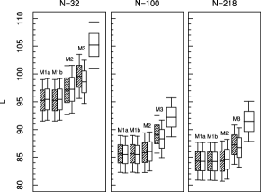
The results of the simulations for the mean function (26) are shown in Figure 4. The data generating processes have exponential covariance functions. If the $\xi_{i}$ in (23) have Gaussian covariances, the results are not visually distinguishable. The errors values for mean (25) are slightly different, but the relative position of the box plots practically does not change. All methods M1, M2 and M3 are significantly better than the sample average. Method M2 strikes the best balance between the computational cost and the precision of estimation. Note that methods M1 and M2 were designed to minimizes the expected $L^{2}$ distance, and all three methods are compared using the $L^{1}$ distance, so this comparison does not a priori favor them. In the context of forecasting, using different loss functions to evaluate the forecasts than to design them can lead to spurious conclusions; see Gneiting (2011). In our context, if the $L^{2}$ distance is used to compare the methods, the ranking and conclusions are the same.

Figure 5: Errors in the estimation of the FPCs for sample sizes: $32$, $100$, $218$. The bold line inside each box plot represents the average value of $L$. The upper and lower sides of rectangles show one standard deviation, and horizontal lines show two standard deviations. The rightmost boxes correspond to the standard method.

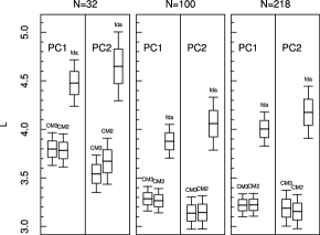
Errors in the estimation of the FPCs in model (27) are shown in Figure 5. The displayed errors are those for the $\xi_{i}$ with exponential covariances and the CH variogram. The results for Gaussian covariances and the MT variogram are practically the same. The performance of methods CM2 and CM3 is comparable, and they are both much better than using the eigenfunctions of the empirical covariance operator (20), which is the standard method implemented in the fda package. The computational complexity of methods CM2 and CM3 is the same.

Conclusions. For simulated data generated to resemble the ionosonde data, all methods introduced in Sections 2 and 3 have integrated absolute deviations (away from a true curve) statistically significantly smaller than the standard methods designed for i.i.d. curves. Methods M2 and CM2, based on weighted averages estimated using functional variograms, offer a computationally efficient and unified approach to the estimation of the mean function and of the FPCs in this spatial setting.

5 Testing for correlation of two spatial fields

Motivated by the problem of testing for correlation between foF2 and magnetic curves, described in detail in Section 8, we now propose a relevant statistical significance test.

There are $N$ spatial locations: $\mathbf{s}_{1},\mathbf{s}_{2},\ldots,\mathbf{s}_{N}$. At location $\mathbf{s}_{k}$, we have two curves:

$$X_{k}=X(\mathbf{s}_{k})=X(\mathbf{s}_{k};t),\qquad t\in[0,1],$$

and

$$Y_{k}=Y(\mathbf{s}_{k})=Y(\mathbf{s}_{k};t),\qquad t\in[0,1].$$

We want to test the null hypothesis that the collections of curves $\{X_{k},1\leq k\leq N\}$ and $\{Y_{k},1\leq k\leq N\}$ are uncorrelated in a sense defined below. The null distribution is derived assuming a stronger condition that these two families are independent. Székely, Rizzo and Bakirov (2007) and Székely and Rizzo (2009) introduced measures of dependence based on the distance of characteristic functions which allow to test independence (rather than just lack of correlation) of random variables $X$ and $Y$ given a sample of i.i.d. observations $(X_{k},Y_{k})$. The extension of their theory to the case of spatially dependent observations $(X_{k},Y_{k})$ is not obvious, so we consider only a test for linear dependence.

The idea of the test is as follows. To lighten the notation, assume that

$$EX_{k}(t)=0\quad\mbox{and}\quad EY_{n}(t)=0.$$

The mean functions will be estimated and subtracted using one of the methods of Section 2. We approximate the curves $X_{n}$ and $Y_{n}$ by the expansions

$$X_{n}(t)\approx\sum_{i=1}^{p}\langle X_{n},v_{i}\rangle v_{i}(t),\qquad Y_{n}(t)\approx\sum_{j=1}^{q}\langle Y_{n},u_{j}\rangle u_{j}(t),$$

where the $v_{i}$ and the $u_{j}$ are the corresponding FPCs. At this point, the functions $v_{i},1\leq i\leq p$ and $u_{j},1\leq j\leq q$ are deterministic, so the independence of the curves $X_{n}$ of the curves $Y_{n}$ implies the independence of the vectors

$$[\langle X_{n},v_{1}\rangle,\langle X_{n},v_{2}\rangle,\ldots,\langle X_{n},v_{p}\rangle]^{T},\qquad 1\leq n\leq N$$

and

$$[\langle Y_{n},u_{1}\rangle,\langle Y_{n},u_{2}\rangle,\ldots,\langle Y_{n},u_{q}\rangle]^{T},\qquad 1\leq n\leq N.$$

Then, under $H_{0}$, the expected value of the sample covariances

$$A_{N}(i,j)=\frac{1}{N}\sum_{n=1}^{N}\langle X_{n},{v}_{i}\rangle\langle Y_{n},{u}_{j}\rangle$$ (32)

is zero. If their estimated versions are large as a group, that is, if some of the estimated $A_{N}(i,j)$ are too large, we reject the null hypothesis.

To construct a test statistic, we introduce the quantities

$$V_{k\ell}(i,{i^{\prime}})=E[\langle v_{i},X_{k}\rangle\langle v_{i^{\prime}},X_{\ell}\rangle],\qquad U_{k\ell}(j,j^{\prime})=E[\langle u_{j},Y_{k}\rangle\langle u_{j}^{\prime},Y_{\ell}\rangle].$$

Note that $V_{k\ell}(i,{i^{\prime}})=0$ and $U_{k\ell}(j,j^{\prime})=0$, if the observations in each sample are independent (and have mean zero). Thus, the $V_{k\ell}(i,{i^{\prime}})$ and the $U_{k\ell}(j,j^{\prime})$ are specific to dependent data, they do not occur in the currently available testing procedures developed for independent curves. Setting $X_{ik}=\langle v_{i},X_{k}\rangle,Y_{jk}=\langle u_{j},Y_{k}\rangle,$ observe that if the $X_{ik}$ are uncorrelated with the $Y_{jk}$, then

$$E\bigl{[}\sqrt{N}A_{N}(i,j)\sqrt{N}A_{N}({i^{\prime}},j^{\prime})\bigr{]} = \frac{1}{N}E\Biggl{[}\sum_{k=1}^{N}X_{ik}Y_{jk}\sum_{\ell=1}^{N}X_{{i^{\prime}}\ell}Y_{j^{\prime}\ell}\Biggr{]}$$

$$= \frac{1}{N}\sum_{k=1}^{N}\sum_{\ell=1}^{N}E[X_{ik}X_{{i^{\prime}}\ell}]E[Y_{jk}Y_{j^{\prime}\ell}]$$

$$= \frac{1}{N}\sum_{k=1}^{N}\sum_{\ell=1}^{N}V_{k\ell}(i,{i^{\prime}})U_{k\ell}(j,j^{\prime}).$$

The normalized covariance tensor of the $\sqrt{N}A_{N}(i,j)$ thus has entries

$${\sigma}_{N}(i,j;{i^{\prime}},j^{\prime})=\frac{1}{N}\sum_{k,\ell=1}^{N}V_{k\ell}(i,{i^{\prime}})U_{k\ell}(j,j^{\prime}).$$ (33)

The idea of the test is to approximate the distribution of the matrix

$$\mathbf{A}_{N}=[A_{N}(i,j),1\leq i\leq p,1\leq j\leq q]$$

via $\sqrt{N}\mathbf{A}_{N}\approx\mathbf{Z},$ where $\mathbf{Z}$ is a $p\times q$ Gaussian matrix whose elements have covariances $E[Z(i,j)Z({i^{\prime}},j^{\prime})]={\sigma}_{N}(i,j;{i^{\prime}},j^{\prime}).$

We now explain how to implement this idea. Denote by $\hat{\lambda}_{i},\hat{\gamma}_{j}$ and ${\hat{v}}_{i},{\hat{u}}_{j}$ the eigenvalues and the eigenfunctions estimated either by method CM2 or CM3. The covariances $A_{N}(i,j)$ are then estimated by

$$\hat{A}_{N}(i,j)=\frac{1}{N}\sum_{n=1}^{N}\langle X_{n},{\hat{v}}_{i}\rangle\langle Y_{n},{\hat{u}}_{j}\rangle.$$

If the observations within each sample are independent, an appropriate test statistic is

$$N\sum_{i=1}^{p}\sum_{j=1}^{q}{\hat{\lambda}_{i}}^{-1}{\hat{\gamma}_{j}}^{-1}\hat{A}_{N}^{2}(i,j).$$

Since ${\lambda}_{i}=E[\langle v_{i},X\rangle^{2}]$, this is essentially the sum of all correlations, and it tends to a chi-squared distribution with $pq$ degrees of freedom, as shown in Kokoszka et al. (2008). This is, however, not that case for dependent data. To explain, set

$$\mathbf{a}_{N}=\operatorname{vec}(\mathbf{A}_{N}),$$

that is, $\mathbf{a}_{N}$ is a column vector of length $pq$ consisting of the columns of $\mathbf{A}_{N}$ stacked on top of each other, starting with the first column. Then $\sqrt{N}\mathbf{a}_{N}$ is approximated by a Gaussian vector $\mathbf{z}$ with covariance matrix ${\bm{\Sigma}}$ constructed from the entries (33). It follows that

$$\hat{S}_{N}=N{\hat{\mathbf{a}}_{N}}^{T}{\hat{\bm{\Sigma}}}^{-1}{\hat{\mathbf{a}}_{N}}\approx\chi^{2}_{pq},$$ (34)

where $\hat{\mathbf{a}}_{N}=\operatorname{vec}(\hat{\mathbf{A}}_{N})$. The entries of the matrix $\hat{\bm{\Sigma}}$ are

$$\hat{\sigma}_{N}(i,j;{i^{\prime}},j^{\prime})=\frac{1}{N}\sum_{k,\ell=1}^{N}{\hat{V}}_{k\ell}(i,{i^{\prime}}){\hat{U}}_{k\ell}(j,j^{\prime}),$$ (35)

where ${\hat{V}}_{k\ell}(i,{i^{\prime}})$ and ${\hat{U}}_{k\ell}(j,j^{\prime})$ are estimators of ${V}_{k\ell}(i,{i^{\prime}})$ and ${U}_{k\ell}(j,j^{\prime})$, respectively. The test rejects $H_{0}$ if $\hat{S}_{N}>\chi^{2}_{pq}(1-{\alpha})$, where $\chi^{2}_{pq}(1-{\alpha})$ is the 100$(1-{\alpha})$th percentile of the chi-squared distribution with $pq$ degrees of freedom. One can use Monte Carlo versions of the above test, for example, the test is based on the approximation

$$\hat{T}_{N}:=N{\hat{\mathbf{a}}_{N}}^{T}{\hat{\mathbf{a}}_{N}}\approx\mathbf{w}^{T}{\hat{\bm{\Sigma}}}\mathbf{w},$$ (36)

where the components of $\mathbf{w}$ are i.i.d. standard normal.

The test procedure can be summarized as follows: [(3)]

Subtract the mean functions, estimated by one of the methods of Section 2, from both samples.

Estimate the FPCs by method CM2 or CM3.

Using a model for the covariance tensor (35) (see Section 6), compute the test statistic $\hat{S}_{N}$. (This tensor is not needed to compute $\hat{T}_{N}$, but it is needed to find its Monte Carlo distribution.)

Find the $P$-value using either a Monte Carlo distribution or the $\chi^{2}$ approximation.

We now turn to the important issue of modeling and estimation of the matrix ${\bm{\Sigma}}$.

6 Modeling and estimation of the covariance tensor

The estimation of the $V_{k\ell}(i,{i^{\prime}})$ involves only the $X_{n}$, and the estimation of the $U_{k\ell}(j,j^{\prime})$ only the $Y_{n}$, so we describe only the procedure for the $V_{k\ell}(i,{i^{\prime}})$. We assume that the mean has been estimated and subtracted, so that we can define

$$C_{h}(x)=E[\langle X(\mathbf{s}),x\rangle X(\mathbf{s}+\mathbf{h})],\qquad h=\|\mathbf{h}\|.$$ (37)

The estimation of the $V_{k\ell}(i,{i^{\prime}})$ relies on the identity

$$V_{k\ell}(i,{i^{\prime}})=\langle C_{h}(v_{i}),v_{{i^{\prime}}}\rangle,\qquad h=d(\mathbf{s}_{k},\mathbf{s}_{\ell}).$$

To propose a practical approach to the estimation of ${\bm{\Sigma}}$, we consider an extension of the multivariate intrinsic model; see, for example, Chapter 22 of Wackernagel (2003). A most direct extension is to assume that

$$C_{h}=Cr(h),$$ (38)

where $C$ is a covariance operator, that is, a symmetric positive definite operator with summable eigenvalues, and $r(h)$ is a correlation function of a scalar random field. Since $r(0)=1$, we have $C=C_{0}$, so $C$ in (38) must be the covariance operator of each $X(\mathbf{s})$. If we assume the intrinsic model (38), then

$$V_{k\ell}(i,j)=\langle r(h)C(v_{i}),v_{j}\rangle={\lambda}_{i}{\delta}_{ij}r(d(\mathbf{s}_{k},\mathbf{s}_{l})).$$ (39)

To allow more modeling flexibility, we postulate that

$$V_{k\ell}(i,j)={\lambda}_{i}{\delta}_{ij}r_{i}(d(\mathbf{s}_{k},\mathbf{s}_{l})).$$ (40)

Under (39) [equivalently, under (38)], each scalar field $\langle X(\mathbf{s}),v_{i}\rangle$ has the same correlation function, only their variances are different. Under (40), the fields $\langle X(\mathbf{s}),v_{i}\rangle$ can have different correlation functions. As will be seen below, model (40) also leads to a valid covariance matrix.

The correlations $r_{i}(d(\mathbf{s}_{k},\mathbf{s}_{l}))$ and the variances ${\lambda}_{i}$ can be estimated using a parametric model for the scalar field $\xi_{i}(\mathbf{s})=\langle X(\mathbf{s}),v_{i}\rangle$. The resulting estimates $\hat{r}_{i}(d(\mathbf{s}_{k},\mathbf{s}_{l}))$ and ${\hat{\lambda}}_{i}$ lead to the estimates $\hat{V}_{k\ell}(i,j)$ via (40). Analogous estimates of the functional field $Y$ are $\hat{\gamma}_{j}(d(\mathbf{s}_{k},\mathbf{s}_{l})),\hat{\tau}_{j}$ and $\hat{U}_{k\ell}(i,j)$.

For ease of reference, we note that under model (40) and $H_{0}$, the covariance tensor,

$$\Biggl{[}\frac{1}{N}\sum_{k=1}^{N}\sum_{\ell=1}^{N}\hat{V}_{k\ell}(i,i^{\prime})\hat{U}_{k\ell}(j,j^{\prime}),1\leq i,i^{\prime}\leq p,1\leq j,j^{\prime}\leq q\Biggr{]},$$

has the following matrix representation:

$$\hat{{\bm{\Sigma}}}=\operatorname{diag}\Biggl{(}\sum_{k=1}^{N}\sum_{\ell=1}^{N}\hat{{\bm{\Sigma}}}_{\xi_{1}}(k,\ell)\hat{{\bm{\Sigma}}}_{\eta_{1}}(k,\ell),\ldots,\sum_{k=1}^{N}\sum_{\ell=1}^{N}\hat{{\bm{\Sigma}}}_{\xi_{p}}(k,\ell)\hat{{\bm{\Sigma}}}_{\eta_{q}}(k,\ell)\Biggr{)},$$ (41)

where

$$\hat{{\bm{\Sigma}}}_{\xi_{i}}(k,\ell)=\frac{1}{\sqrt{N}}\hat{\lambda}_{i}\hat{r}_{i}(d(\mathbf{s}_{k},\mathbf{s}_{\ell}))$$

and

$$\hat{{\bm{\Sigma}}}_{\eta_{j}}(k,\ell)=\frac{1}{\sqrt{N}}\hat{\gamma}_{j}\hat{\tau}_{j}(d(\mathbf{s}_{k},\mathbf{s}_{\ell})).$$

This form is used to construct the Monte Carlo tests discussed in Section 7.

The matrices ${\bm{\Sigma}}$ and $\widehat{\bm{\Sigma}}$ are positive definite; see Horváth and Kokoszka (2012) for the verification.

7 Size and power of the correlation test

As in Section 4, our objective is to evaluate the finite sample performance of the test introduced in Section 5 in a realistic setting geared toward the application presented in Section 8.

Table 1: Models and estimated covariance parameters for the transformed foF2 curves and the magnetic curves

		Parameters
Spatial
field	Model	$\bm{c_{0}}$	$\bm{\sigma^{2}}$	$\bm{\rho}$
$\bm{\eta}$	Gaussian	–	$5.99\pm 0.48$	$0.32\pm 0.04$
$\bm{\xi}_{1}$	Gaussian	–	$20.05\pm 2.20$	$0.12\pm 0.03$
$\bm{\xi}_{2}$	–	–	$3.30\pm 0.43$	–
$\bm{\xi}_{3}$	Exponential	–	$2.63\pm 0.52$	$0.16\pm 0.07$
$\bm{\xi}_{4}$	Gaussian	–	$2.66\pm 0.39$	$0.18\pm 0.05$
$\bm{\xi}_{5}$	–	–	$2.74\pm 0.32$	–
$\bm{\xi}_{6}$	Gaussian	$0.16\pm 0.02$	$0.85\pm 0.24$	$0.17\pm 0.06$
$\bm{\xi}_{7}$	–	–	$1.22\pm 0.18$	–

Data generating processes. We generate samples of zero mean Gaussian processes

$$X(\mathbf{s};t)=\sum_{i=1}^{p}\xi_{i}(\mathbf{s})v_{i}(t);\qquad Y(\mathbf{s};t)=\sum_{j=1}^{q}\eta_{j}(\mathbf{s})u_{j}(t).$$ (42)

The process $X$ is designed to resemble in distribution appropriately transformed and centered foF2 curves; the process $Y$ the centered magnetic curves. Following the derivation presented in Section 8, we use $p=7$ and $q=1$. The curves $v_{i}$ and $u_{1}$ are the estimated FPCs of the real data. The scalar Gaussian spatial fields $\xi_{i}$ and $\eta_{1}$ follow parametric models estimated for real data; details of the models are presented in Table 1. The $\xi_{i}$ are independent. Under $H_{0}$, the $\xi_{i}$ are independent of $\eta_{1}$. The dependence under $H_{A}$ can be generated in many ways. We considered the following scenarios: $\xi_{1}$ and $\eta_{1}$ are dependent, $\xi_{i}$ and $\eta_{1}$ are independent for $i\neq 1$, then $\xi_{2}$ and $\eta_{1}$ are dependent, $\xi_{i}$ and $\eta_{1}$ are independent for $i\neq 2$, etc. To produce two dependent spatial fields $\xi_{i}$ and $\eta$, we generated $N$ i.i.d. pairs $\mathbf{x}_{i}=[x_{1i},x_{2i}]^{T}$, $1\leq i\leq N$, where

$$\mathbf{x}_{i}\sim N\left(\mathbf{0},\pmatrix{1&\rho\cr\rho&1}\right).$$

Then we merged all $x_{1i}$ into vector $\mathbf{y}_{1}=[x_{11},\ldots,x_{1N}]^{T}$ and all $x_{2i}$ into vector $\mathbf{y}_{2}=[x_{21},\ldots,x_{2N}]^{T}$. Performing the Cholesky rotation, we obtain correlated spatial vectors:

$$\bm{\xi}_{i}=\mathbf{V}\mathbf{y}_{1},\qquad({\bm{\Sigma}}_{\xi_{i}}=\mathbf{V}\mathbf{V}^{T}),\qquad\bm{\eta}=\mathbf{U}\mathbf{y}_{2},\qquad({\bm{\Sigma}}_{\eta}=\mathbf{U}\mathbf{U}^{T}).$$

We used sample sizes $N=32$ and $N=100$ corresponding to the locations determined as in Section 4.

Testing procedures. We studied the finite sample behavior of three methods, which we call S, SM and T. Method S rejects $H_{0}$ if the statistic $\hat{S}_{N}$ (34) exceeds a chi-square critical value. Method SM uses a Monte Carlo distribution of the statistic $\hat{S}_{N}$: after estimating all parameters from the data and assuming the Gaussian distribution of the fields $\xi_{i}$ and $\eta_{1}$, we can replicate the values of the statistic $\hat{S}_{N}$ under $H_{0}$ using the covariance matrix (41). Method T uses the statistics $\hat{T}_{N}$ (36), and approximates its distribution by the Monte Carlo distribution of $\mathbf{w}^{T}\hat{\bm{\Sigma}}\mathbf{w}$, as explained in Section 5. For determining the critical values in methods SM and T, we used $10^{7}$ Monte Carlo replications. The empirical size and power are based on $10^{5}$ independent runs.

Figure 6: Size of the correlation test as a function of $p$. Solid disks represent method S (based on $\chi^{2}$ distribution). Circles represent method SM (based on the Monte Carlo distribution).

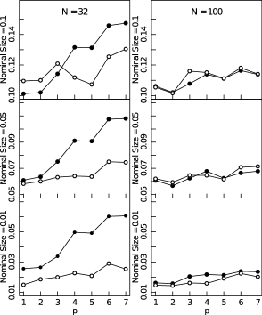
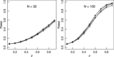
Conclusions. As Figure 6 shows, the empirical size is higher than the nominal size, and it tends to increase with the number $p$ of principal components used to construct the test, especially for $N=32$. The usual recommendation is to use $p$, which explains about 85% of the variance. For the foF2 data with $N=32$, this corresponds to $p=4$. Applied to real data in Section 8, all tests (S, SM and T) lead to extremely strong rejections, so the inflated empirical size is not a problem. Figure 6 also shows that the Monte Carlo approximation is useful for $N=32$, this is the sample size we must use in Section 8. The size of test T is practically indistinguishable from that of test SM. Figure 7 shows the power of method SM; power curves for method T are practically the same, method S has higher power. The simulation study shows that a strong rejection when the test is applied to real data can be viewed as reliable evidence of dependence.

8 Application to critical ionospheric frequency and magnetic curves

In this section we apply the correlation test, which uses the estimation methodology of Sections 2 and 3, to foF2 and magnetic curves.

Figure 7: Power of the correlation test SM as a function of the population correlation $\rho$. Each line represents one of the four possible correlated spatial fields: $\bm{\xi}_{1}-\bm{\eta}$, $\bm{\xi}_{2}-\bm{\eta}$, $\bm{\xi}_{3}-\bm{\eta}$, $\bm{\xi}_{4}-\bm{\eta}$. The test was performed using $p=4$, which explains about $85\%$ of variance of the foF2 curves. Since all curves in the graphs are practically the same, we do not specify which curve represents a particular dependent pair $\bm{\xi}_{i}-\bm{\eta}$.

Description of the data. The F2 layer of the ionosphere is the upper part of the F layer shown in Figure 3. The F2 layer electron critical frequency, foF2, is measured using an instrument called the ionosonde, a type of radar. The foF2 frequency is used to estimate the location of the peak electron density, so an foF2 trend corresponds to a trend in the average height of the ionosphere over a spatial location. The foF2 data have therefore been used to test the hypothesis of ionospheric global cooling discussed in the Introduction. Hourly values of foF2 are available from the SPIDR database http://spidr.ngdc.noaa.gov/spidr/ for more than 200 ionosondes. We use monthly averages for 32 selected ionosondes, with sufficiently complete records, for the period 1964–1992. Their locations are shown in Figure 2. Three typical foF2 curves are shown in Figure 1. We omit the details of the procedure for obtaining curves like those shown in Figure 1, but we emphasize that it requires a great deal of work. In particular, the SPIDR data suffer from two problems. First, for some data, the amplitude is artificially magnified ten times, and needs to be converted into standard units (MHz). Second, in many cases, missing observations are not replaced by the standard notation $9999$, but rather just skipped. Thus, if one wants to use equally-spaced time series, skipped data must be found and replaced by missing values. For filling in missing values, we perform linear interpolation. We developed a customized C++ code to handle these issues. We emphasize that one of the reasons why this global data set has not been analyzed so far is that useable data have been derived only over relatively small regions, for example, Western Europe, and more often for a single location.

Figure 8: Dots represent the scaling function $G_{L}(\mathbf{s}_{i})$ in the magnetic coordinate system and crosses are the same in the geographic coordinate system. Line is the best fit for $G_{L}$ in the magnetic coordinate system.

As explained in Section 1, the foF2 data are used to test hypotheses on long-term ionospheric trends. We thus removed annual and higher frequency variations using $16$ month averaging with MODWT filter; see Chapter 5 of Percival and Walden (2000). This leads to 32 time series at different locations, each containing $336$ equally-spaced temporal observations. The amplitude of the foF2 curves exhibits a nonlinear latitudinal trend; it decreases as the latitude increases; see Figure 1. To remove this trend, which may potentially bias the test, we assume that the foF2 signal, $F(\mathbf{s};t)$, at location $\mathbf{s}$ follows the model

$$F(\mathbf{s};t)=G(L(\mathbf{s}))X(\mathbf{s};t),$$ (43)

where $X(\mathbf{s};t)$ is a constant amplitude field, and $G(\cdot)$ is a scaling function which depends only on the magnetic latitude $L$ (in radians). Since the trend in the amplitude of $F(\mathbf{s};t)$ is caused by the solar radiation which is nonlinearly proportional to the zenith angle, we postulate that the function $G(\cdot)$ has the form

$$G(L)=a+b\cos^{c}(L).$$ (44)

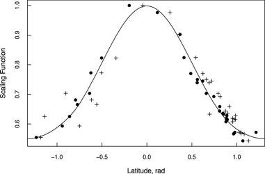
The parameters $a,b,c$ are estimated as follows. Let $\mathbf{s}_{0}$ be the position of the ionosonde closest to the magnetic equator. For identifiability, we set $G(L(\mathbf{s}_{0}))=1$. For the remaining locations $\mathbf{s}_{k}$, we compute $\hat{G}(L(\mathbf{s}_{k}))$ as the average, over all 336 time points $t_{j}$ of the ratio $F(\mathbf{s}_{k};t_{j})/F(\mathbf{s}_{0};t_{j})$. Figure 8 shows these ratios as a function of the magnetic and geographic latitude. The ratios in the magnetic latitude show much less spread, and this is another reason why we work with the magnetic latitude. The curve $G(L)$ (44) is fitted to the $\hat{G}(L(\mathbf{s}_{k}))$ in magnetic latitude by nonlinear least squares. The fitted values are $a=0.5495$, $b=0.4488$, $c=4.2631$.

We now describe how we construct the curves that reflect the relevant long-term changes in the internal magnetic field of the earth. The height of the F2 layer (and so the foF2 frequency) can be affected by a vertical plasma drift which responds to the magnetic field. The vertical plasma drift is due to the wind effect, and is given by [we use the same notation as in Mikhailov and Marin (2001)]

$$W=(V_{nx}\cos D-V_{ny}\sin D)\sin I\cos I+V_{nz}\sin^{2}I.$$

In the above formula, $V_{nx}$, $V_{ny}$ and $V_{nz}$ are, respectively, meridional (parallel to constant longitude lines), zonal (parallel to constant latitude lines) and vertical components of the thermospheric neutral wind; $I$ and $D$ are inclination and declination of the earth magnetic field. Detailed figures are provided in Chapter 13 of Kivelson and Russell (1997). Usually $V_{nz}\ll V_{nx},V_{ny},$ and assuming that the difference between magnetic and geographic coordinates, $D$, is small (at least for low- and mid-latitude regions), we can simplify the above formula to $W=V_{nx}\sin I\cos I.$ Thus, only the meridional thermospheric wind is significant. Measuring neutral wind components ($V_{nx}$, $V_{ny}$, $V_{nz}$) is difficult, and long-term wind records are not available. We therefore replace $V_{nx}$ by its average. For the test of correlation, the specific value of this average plays no role, so we define the magnetic curves as

$$Y(\mathbf{s};t)=\sin I(\mathbf{s};t)\cos I(\mathbf{s};t).$$ (45)

The curves $I(\mathbf{s};t)$ are computed using the international geomagnetic reference field (IGRF); the software is available at http://www.ngdc.noaa.gov/ IAGA/vmod/.

The test is applied to the curves $X(\mathbf{s}_{k};t)$ defined by (43) and (44), and to the curves $Y(\mathbf{s}_{k};t)$ defined by (45).

Application of the correlation test. We first estimate and subtract the mean functions of the fields $X(\mathbf{s}_{k})$ and $Y(\mathbf{s}_{k})$ using method M2 (the other spatial methods give practically the same estimates). The principal components $v_{i}$ and $u_{i}$ are estimated using method CM2 (method CM3 gives practically the same curves).

Figure 9: Transformed and centered foF2 curves (continuous) and centered magnetic curves (dashed) at 32 locations denoted with circles in Figure 2. The scales for the two families of curves are different. The foF2 curves have the same scale, it is shown on the right vertical axes in MHz. The scale of the magnetic curves changes, it is shown on the right vertical axes in each box (unitless).

Table 2: $P$-values of the correlation tests applied to the transformed foF2 data. The first column shows the number of FPCs, the second column shows cumulative variances computed as the ratios of the eigenvalues estimated using method CM2. Testing procedures S, SM and T are defined in Section 7. The “simple” procedure neglects the spatial dependence of the curves

		Spatial
$\bm{p}$	CV, $\bm{\%}$	S	SM	T	Simple
1	47.88	$6.22\cdot 10^{-5}$1	$3.05\cdot 10^{-4}$	$3.05\cdot 10^{-4}$	$0.035$
2	62.59	$3.26\cdot 10^{-6}$1	$2.91\cdot 10^{-4}$	$2.99\cdot 10^{-4}$	$0.095$
3	73.67	$4.53\cdot 10^{-8}$1	$2.43\cdot 10^{-4}$	$2.32\cdot 10^{-4}$	$0.043$
4	84.40	$1.47\cdot 10^{-26}$	$1.6\cdot 10^{-7}$0	$2.24\cdot 10^{-5}$	$0.039$
5	88.70	$4.95\cdot 10^{-26}$	$2.6\cdot 10^{-7}$0	$2.27\cdot 10^{-5}$	$0.046$
6	92.21	$6.73\cdot 10^{-27}$	$5.9\cdot 10^{-7}$0	$2.21\cdot 10^{-5}$	$0.060$
7	94.57	$2.12\cdot 10^{-32}$	$1.6\cdot 10^{-7}$0	$1.92\cdot 10^{-5}$	$0.030$

We apply the test, for all $1\leq p\leq 7$ and $q=1$. The first seven eigenvalues of the field $X$ [computed per (17) or its analog for method CM2] explain about 95% of the variance. The first eigenvalue of the field $Y$ explains about 99% of the variance. The eigenfunction $u_{1}$ is approximately equal to the linear function: $u_{1}(t)\sim t$. This means that at any location, after removing the average, the magnetic field either linearly increases or decreases, with slopes depending on the location; see Figure 9. To lighten the notation, we drop the “hats” from the estimated scores and denote the zero mean vector $[xi_{i}(\mathbf{s}_{1}),\ldots,\xi_{i}(\mathbf{s}_{N})]^{T}$ by $\bm{\xi}_{i}$, and $[\eta_{1}(\mathbf{s}_{1}),\ldots,\eta_{1}(\mathbf{s}_{N})]^{T}$ by $\bm{\eta}$. The covariances ${\bm{\Sigma}}_{\xi_{i}}$ and ${\bm{\Sigma}}_{\eta}$ are estimated using parametric spatial models determined by the inspection of the empirical variograms. In this application, it is sufficient to use two covariance models:

$$\mbox{Gaussian:}\ c(\mathbf{s}_{k},\mathbf{s}_{\ell})=c_{0}+\sigma^{2}\exp\{-d^{2}(k,\ell)/\rho^{2}\},$$

(46)

$$\mbox{Exponential:}\ c(\mathbf{s}_{k},\mathbf{s}_{\ell})=c_{0}+\sigma^{2}\exp\{-d(k,\ell)/\rho\}.$$

When the scores do not have a spatial structure, we use the sample variance (flat variogram). The estimated models and their parameters are listed in Table 1.

The $P$-values for different numbers of FPCs $1\leq p\leq 7$ are summarized in Table 2. Independent of $p$ and a specific implementation of the test, all $P$-values are very small, and so the rejection of the null hypothesis is conclusive; we conclude that there is a statistically significant correlation between the foF2 curves $X(\mathbf{s}_{k})$ and the magnetic curves $Y(\mathbf{s}_{k})$. We also applied a version of our test which neglects any spatial dependence, this is the test proposed by Kokoszka et al. (2008). The $P$-values hover around the 5% level, but still point toward rejection. The evidence is, however, much less clear cut. This may partially explain why this issue has been a matter of much debate in the space physics community. The correlation between the foF2 and magnetic curves is far from obvious. Figure 9 shows these pairs at all 32 locations. It is hard to conclude by eye that the direction of the magnetic field change impacts the foF2 curves.

Discussion. A very important role in our analysis is played by the transformation (44). Applying the test to the original foF2 curves, $F(\mathbf{s}_{k};t)$, gives the $P$-values 0.209 ($p=1$) and 0.011 ($p=2$) for the spatial S test, and 0.707 ($p=1$), 0.185 ($p=2$), 0.139 ($p=3$) for the “simple” test. As explained above, the amplitude of the field $F(\mathbf{s}_{k};t)$ evolves with the latitude. This invalidates the assumption of a mean function which is independent of the spatial location. Thus, even for the spatial test, the mean function confounds the first FPC. However, the spatial estimation of the mean function and of the FPCs “quickly corrects” for the violation of assumptions, and the null hypothesis is rejected for $p\geq 2$. When the spatial structure is neglected (and no latitudinal transformation is applied) no correlation between the foF2 curves and magnetic curves is found.

Figure 10: Scatter plots of the scores $\bm{\xi}_{i},i=1,2,3,4$ of the foF2 curves, vertical axes, against the scores $\bm{\eta}$ of the magnetic curves, horizontal axes.

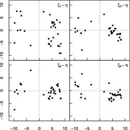
The rejection of the null hypothesis means that after adjusting the foF2 curves for the latitude and the global mean, their regional variability is correlated with the regional changes in the magnetic field. This conclusion agrees with recent space physics research [see Cnossen and Richmond (2008) and Laštovička (2009)], and can, to some extent, be visually confirmed, post-analysis, by the examination of the scatter plots shown in Figure 10. It implies that long-term magnetic trends must be considered as additional covariates in testing for long-term trends in the foF2 curves. The main covariate is the solar activity which drives the shape of the mean function, but, as explained in the Introduction, the impact of the concentration of the greenhouse gases is of particular interest; see Qian et al. (2009), among many other contributions.

A broader conclusion of the work presented in this paper is that methods of functional data analysis must be applied with care to curves obtained at spatial locations. Neglecting the spatial dependence can lead to incorrect conclusions and biased estimates. The same applies to space physics research. If trends or models are estimated separately at each spatial location, one should not rely on results obtained by some form of a simple averaging. This is, however, the prevailing approach. Interestingly, the results related to global ionospheric trends are often on the borderline of statistical significance. Standard $t$-tests lead either to rejection or acceptance, depending on a specific method used (a similar phenomenon is observed in the last column of Table 2). It is hoped that the methodology developed in this paper will be useful in addressing such issues.

References

- Bel et al. (2011) {barticle}[mr] \bauthor\bsnmBel, \bfnmLiliane\binitsL., \bauthor\bsnmBar-Hen, \bfnmAvner\binitsA., \bauthor\bsnmPetit, \bfnmRémy\binitsR. and \bauthor\bsnmCheddadi, \bfnmRachid\binitsR. (\byear2011). \btitleSpatio-temporal functional regression on paleoecological data. \bjournalJ. Appl. Stat. \bvolume38 \bpages695–704. \biddoi=10.1080/02664760903563650, issn=0266-4763, mr=2773575 \bptokimsref \endbibitem
- Cnossen and Richmond (2008) {barticle}[auto:STB—2012/01/27—08:30:54] \bauthor\bsnmCnossen, \bfnmI.\binitsI. and \bauthor\bsnmRichmond, \bfnmA. D.\binitsA. D. (\byear2008). \btitleModelling the effects of changes in the Earth’s magnetic field from 1957 to 1997 on the ionospheric hmF2 and foF2 parameters. \bjournalJournal of Atmospheric and Solar-Terrestrial Physics \bvolume70 \bpages1512–1524. \bptokimsref \endbibitem
- Delicado et al. (2010) {barticle}[mr] \bauthor\bsnmDelicado, \bfnmP.\binitsP., \bauthor\bsnmGiraldo, \bfnmR.\binitsR., \bauthor\bsnmComas, \bfnmC.\binitsC. and \bauthor\bsnmMateu, \bfnmJ.\binitsJ. (\byear2010). \btitleStatistics for spatial functional data: Some recent contributions. \bjournalEnvironmetrics \bvolume21 \bpages224–239. \bidissn=1180-4009, mr=2842240 \bptokimsref \endbibitem
- Finkenstädt, Held and Isham (2007) {bbook}[mr] \beditor\bsnmFinkenstädt, \bfnmBärbel\binitsB., \beditor\bsnmHeld, \bfnmLeonhard\binitsL. and \beditor\bsnmIsham, \bfnmValerie\binitsV., eds. (\byear2007). \btitleStatistical Methods for Spatio-Temporal Systems. \bseriesMonographs on Statistics and Applied Probability \bvolume107. \bpublisherChapman & Hall/CRC, \baddressBoca Raton, FL. \bidmr=2307967 \bptokimsref \endbibitem
- Gelfand et al. (2010) {bbook}[mr] \beditor\bsnmGelfand, \bfnmAlan E.\binitsA. E., \beditor\bsnmDiggle, \bfnmPeter J.\binitsP. J., \beditor\bsnmFuentes, \bfnmMontserrat\binitsM. and \beditor\bsnmGuttorp, \bfnmPeter\binitsP., eds. (\byear2010). \btitleHandbook of Spatial Statistics. \bpublisherCRC Press, \baddressBoca Raton, FL. \bidmr=2761512 \bptokimsref \endbibitem
- Giraldo, Delicado and Mateu (2011a) {barticle}[auto:STB—2012/01/27—08:30:54] \bauthor\bsnmGiraldo, \bfnmR.\binitsR., \bauthor\bsnmDelicado, \bfnmP.\binitsP. and \bauthor\bsnmMateu, \bfnmJ.\binitsJ. (\byear2011a). \btitleOrdinary kriging for function-valued spatial data. \bjournalEnviron. Ecol. Stat. \bvolume18 \bpages411–426. \bptokimsref \endbibitem
- Giraldo, Delicado and Mateu (2011b) {bmisc}[auto:STB—2012/01/27—08:30:54] \bauthor\bsnmGiraldo, \bfnmR.\binitsR., \bauthor\bsnmDelicado, \bfnmP.\binitsP. and \bauthor\bsnmMateu, \bfnmJ.\binitsJ. (\byear2011b). \bhowpublishedA generalization of cokriging and multivariable spatial prediction for functional data. Technical report, Univ. Politécnica de Catalunya, Barcelona. \bptokimsref \endbibitem
- Gneiting (2011) {barticle}[auto:STB—2012/01/27—08:30:54] \bauthor\bsnmGneiting, \bfnmT.\binitsT. (\byear2011). \btitleMaking and evaluating point forecasts. \bjournalJ. Amer. Statist. Assoc. \bvolume106 \bpages746–762. \bptokimsref \endbibitem
- Hörmann and Kokoszka (2012) {bmisc}[auto:STB—2012/01/27—08:30:54] \bauthor\bsnmHörmann, \bfnmS.\binitsS. and \bauthor\bsnmKokoszka, \bfnmP.\binitsP. (\byear2012). \bhowpublishedConsistency of the mean and the principal components of spatially distributed functional data. Bernoulli. To appear. \bptokimsref \endbibitem
- Horváth and Kokoszka (2012) {bbook}[auto:STB—2012/01/27—08:30:54] \bauthor\bsnmHorváth, \bfnmL.\binitsL. and \bauthor\bsnmKokoszka, \bfnmP.\binitsP. (\byear2012). \btitleInference for Functional Data with Applications. \bpublisherSpringer, \baddressBerlin. \bptokimsref \endbibitem
- Kivelson and Russell (1997) {bbook}[mr] \beditor\bsnmKivelson, \bfnmM. G.\binitsM. G. and \beditor\bsnmRussell, \bfnmC. T.\binitsC. T., eds. (\byear1997). \btitleIntroduction to Space Physics. \bpublisherCambridge Univ. Press, \baddressCambridge. \bptokimsref \endbibitem
- Kokoszka et al. (2008) {barticle}[mr] \bauthor\bsnmKokoszka, \bfnmPiotr\binitsP., \bauthor\bsnmMaslova, \bfnmInga\binitsI., \bauthor\bsnmSojka, \bfnmJan\binitsJ. and \bauthor\bsnmZhu, \bfnmLie\binitsL. (\byear2008). \btitleTesting for lack of dependence in the functional linear model. \bjournalCanad. J. Statist. \bvolume36 \bpages207–222. \biddoi=10.1002/cjs.5550360203, issn=0319-5724, mr=2431682 \bptokimsref \endbibitem
- Laštovička (2009) {barticle}[auto:STB—2012/01/27—08:30:54] \bauthor\bsnmLaštovička, \bfnmJ.\binitsJ. (\byear2009). \btitleGlobal pattern of trends in the upper atmosphere and ionosphere: Recent progress. Journal of Atmospheric and Solar-Terrestrial. \bjournalPhysics \bvolume71 \bpages1514–1528. \bptokimsref \endbibitem
- Laštovička et al. (2008) {barticle}[auto:STB—2012/01/27—08:30:54] \bauthor\bsnmLaštovička, \bfnmJ.\binitsJ., \bauthor\bsnmAkmaev, \bfnmR. A.\binitsR. A., \bauthor\bsnmBeig, \bfnmG.\binitsG., \bauthor\bsnmBremer, \bfnmJ.\binitsJ., \bauthor\bsnmEmmert, \bfnmJ. T.\binitsJ. T., \bauthor\bsnmJacobi, \bfnmC.\binitsC., \bauthor\bsnmJarvis, \bfnmJ. M.\binitsJ. M., \bauthor\bsnmNedoluha, \bfnmG.\binitsG., \bauthor\bsnmPortnyagin, \bfnmYu. I.\binitsY. I. and \bauthor\bsnmUlich, \bfnmT.\binitsT. (\byear2008). \btitleEmerging pattern of global change in the upper atmosphere and ionosphere. \bjournalAnnales Geophysicae \bvolume26 \bpages1255–1268. \bptokimsref \endbibitem
- Maslova et al. (2009) {barticle}[auto:STB—2012/01/27—08:30:54] \bauthor\bsnmMaslova, \bfnmI.\binitsI., \bauthor\bsnmKokoszka, \bfnmP.\binitsP., \bauthor\bsnmSojka, \bfnmJ.\binitsJ. and \bauthor\bsnmZhu, \bfnmL.\binitsL. (\byear2009). \btitleRemoval of nonconstant daily variation by means of wavelet and functional data analysis. \bjournalJournal of Geophysical Research \bvolume114 \bpagesA03202. \bptokimsref \endbibitem
- Maslova et al. (2010a) {barticle}[auto:STB—2012/01/27—08:30:54] \bauthor\bsnmMaslova, \bfnmI.\binitsI., \bauthor\bsnmKokoszka, \bfnmP.\binitsP., \bauthor\bsnmSojka, \bfnmJ.\binitsJ. and \bauthor\bsnmZhu, \bfnmL.\binitsL. (\byear2010a). \btitleEstimation of Sq variation by means of multiresolution and principal component analyses. \bjournalJournal of Atmospheric and Solar-Terrestial Physics \bvolume72 \bpages625–632. \bptokimsref \endbibitem
- Maslova et al. (2010b) {barticle}[auto:STB—2012/01/27—08:30:54] \bauthor\bsnmMaslova, \bfnmI.\binitsI., \bauthor\bsnmKokoszka, \bfnmP.\binitsP., \bauthor\bsnmSojka, \bfnmJ.\binitsJ. and \bauthor\bsnmZhu, \bfnmL.\binitsL. (\byear2010b). \btitleStatistical significance testing for the association of magnetometer records at high-, mid- and low latitudes during substorm days. \bjournalPlanetary and Space Science \bvolume58 \bpages437–445. \bptokimsref \endbibitem
- Mikhailov and Marin (2001) {barticle}[auto:STB—2012/01/27—08:30:54] \bauthor\bsnmMikhailov, \bfnmA. V.\binitsA. V. and \bauthor\bsnmMarin, \bfnmD.\binitsD. (\byear2001). \btitleAn interpretation of the foF2 and hmF2 long-term trends in the framework of the geomagnetic control concept. \bjournalAnnales Geophysicae \bvolume19 \bpages733–748. \bptokimsref \endbibitem
- Nerini, Monestiez and Manté (2010) {barticle}[mr] \bauthor\bsnmNerini, \bfnmDavid\binitsD., \bauthor\bsnmMonestiez, \bfnmPascal\binitsP. and \bauthor\bsnmManté, \bfnmClaude\binitsC. (\byear2010). \btitleCokriging for spatial functional data. \bjournalJ. Multivariate Anal. \bvolume101 \bpages409–418. \biddoi=10.1016/j.jmva.2009.03.005, issn=0047-259X, mr=2564350 \bptokimsref \endbibitem
- Percival and Walden (2000) {bbook}[mr] \bauthor\bsnmPercival, \bfnmDonald B.\binitsD. B. and \bauthor\bsnmWalden, \bfnmAndrew T.\binitsA. T. (\byear2000). \btitleWavelet Methods for Time Series Analysis. \bseriesCambridge Series in Statistical and Probabilistic Mathematics \bvolume4. \bpublisherCambridge Univ. Press, \baddressCambridge. \bidmr=1770693 \bptokimsref \endbibitem
- Qian et al. (2009) {barticle}[auto:STB—2012/01/27—08:30:54] \bauthor\bsnmQian, \bfnmL.\binitsL., \bauthor\bsnmBurns, \bfnmA. G.\binitsA. G., \bauthor\bsnmSolomon, \bfnmS. C.\binitsS. C. and \bauthor\bsnmRoble, \bfnmR. G.\binitsR. G. (\byear2009). \btitleThe effect of carbon dioxide cooling on trends in the F2-layer ionosphere. \bjournalJournal of Atmospheric and Solar-Terrestrial Physics \bvolume71 \bpages1592–1601. \bptokimsref \endbibitem
- Ramsay, Hooker and Graves (2009) {bbook}[auto:STB—2012/01/27—08:30:54] \bauthor\bsnmRamsay, \bfnmJ.\binitsJ., \bauthor\bsnmHooker, \bfnmG.\binitsG. and \bauthor\bsnmGraves, \bfnmS.\binitsS. (\byear2009). \btitleFunctional Data Analysis with R and MATLAB. \bpublisherSpringer, \baddressNew York. \bptokimsref \endbibitem
- Rishbeth (1990) {barticle}[auto:STB—2012/01/27—08:30:54] \bauthor\bsnmRishbeth, \bfnmH.\binitsH. (\byear1990). \btitleA greenhouse effect in the ionosphere? \bjournalPlanetary and Space Science \bvolume38 \bpages945–948. \bptokimsref \endbibitem
- Roble and Dickinson (1989) {barticle}[auto:STB—2012/01/27—08:30:54] \bauthor\bsnmRoble, \bfnmR. G.\binitsR. G. and \bauthor\bsnmDickinson, \bfnmR. E.\binitsR. E. (\byear1989). \btitleHow will changes in carbon dioxide and methane modify the mean structure of the mesosphere and thermosphere? \bjournalGeophysical Research Letters \bvolume16 \bpages1441–1444. \bptokimsref \endbibitem
- Schabenberger and Gotway (2005) {bbook}[mr] \bauthor\bsnmSchabenberger, \bfnmOliver\binitsO. and \bauthor\bsnmGotway, \bfnmCarol A.\binitsC. A. (\byear2005). \btitleStatistical Methods for Spatial Data Analysis. \bpublisherChapman & Hall/CRC, \baddressBoca Raton, FL. \bidmr=2134116 \bptokimsref \endbibitem
- Székely, Rizzo and Bakirov (2007) {barticle}[mr] \bauthor\bsnmSzékely, \bfnmGábor J.\binitsG. J., \bauthor\bsnmRizzo, \bfnmMaria L.\binitsM. L. and \bauthor\bsnmBakirov, \bfnmNail K.\binitsN. K. (\byear2007). \btitleMeasuring and testing dependence by correlation of distances. \bjournalAnn. Statist. \bvolume35 \bpages2769–2794. \biddoi=10.1214/009053607000000505, issn=0090-5364, mr=2382665 \bptokimsref \endbibitem
- Székely and Rizzo (2009) {barticle}[mr] \bauthor\bsnmSzékely, \bfnmGábor J.\binitsG. J. and \bauthor\bsnmRizzo, \bfnmMaria L.\binitsM. L. (\byear2009). \btitleBrownian distance covariance. \bjournalAnn. Appl. Stat. \bvolume3 \bpages1236–1265. \biddoi=10.1214/09-AOAS312, issn=1932-6157, mr=2752127 \bptokimsref \endbibitem
- Ulich, Clilverd and Rishbeth (2003) {barticle}[auto:STB—2012/01/27—08:30:54] \bauthor\bsnmUlich, \bfnmT.\binitsT., \bauthor\bsnmClilverd, \bfnmM. A.\binitsM. A. and \bauthor\bsnmRishbeth, \bfnmH.\binitsH. (\byear2003). \btitleDetermining long-term change in the ionosphere. \bjournalEos, Transactions American Geophysical Union \bvolume84 \bpages581–585. \bptokimsref \endbibitem
- Wackernagel (2003) {bbook}[auto:STB—2012/01/27—08:30:54] \bauthor\bsnmWackernagel, \bfnmH.\binitsH. (\byear2003). \btitleMultivariate Geostatistics, \bedition3rd ed. \bpublisherSpringer, \baddressNew York. \bptokimsref \endbibitem
- Yamanishi and Tanaka (2003) {barticle}[mr] \bauthor\bsnmYamanishi, \bfnmYoshihiro\binitsY. and \bauthor\bsnmTanaka, \bfnmYutaka\binitsY. (\byear2003). \btitleGeographically weighted functional multiple regression analysis: A numerical investigation. \bjournalJ. Japanese Soc. Comput. Statist. \bvolume15 \bpages307–317. \bidissn=0915-2350, mr=2027947 \bptokimsref \endbibitem