LHC and dark matter signals of bosons
Abstract
We customize the simulation code FEWZ (Fully Exclusive W, Z Production) to study production at the LHC for both TeV and 14 TeV. Using the results of our simulation for several standard benchmark models, we derive a semi-empirical expression for the differential cross section, that permits the determination of couplings in a model-independent manner. We evaluate cross sections and other observables for large classes of models, including the common , left-right and models, as a function of model parameters. We also consider a hidden sector that couples to standard model fermions via kinetic and mass mixing and serves as a mediator of isospin-violating interactions with dark matter. We combine the results of LHC searches and dark matter direct detection experiments with global electroweak data to obtain mass-dependent constraints on the model parameters.
I Introduction
A simple extension of the Standard Model (SM) is the addition of an extra gauge symmetry, with associated neutral gauge boson. Extra symmetries are a necessary part of many interesting new physics scenarios, including several Grand Unified Theories and string-inspired model constructions. Generic models can have many new physics features, including generation-dependent couplings, mixing, and new fermions; see e.g., Refs. Langacker:2008yv ; Carena:2004xs ; Leike:1998wr ; Hewett:1988xc ; London:1986dk . We first study the simplest models with generation-independent couplings and no mixing. There are a number of such models that are theoretically relevant, such as the GUT models and the model. In Section VI, we consider a model that includes mass and kinetic mixing between the and the Frandsen:2011cg , which has applications to isospin-violating dark matter scattering Feng:2011vu .
We expand the simulation code FEWZ 2.1 Gavin:2012kw ; Gavin:2010az to study the production and decay of bosons at the LHC through the process . FEWZ includes up to NNLO in perturbative QCD and is fully differential in the lepton phase space. This allows for the precise calculation of the cross sections and differential distributions with realistic experimental acceptances. In Sections II and III, we briefly review detection and introduce several common benchmark models that we use to demonstrate the efficacy and validity of our simulation.
In Section IV we use FEWZ to derive a semi-empirical expression for the differential cross section . We show that, with sufficient data, this formula can be used to determine the couplings of the and set limits on model parameters with good precision.
In Section V, we apply our fit to the model class and the production of two bosons. The heavier of the two mass eigenstates is often assumed to be too heavy for collider detection, but we show that it could be accessible at the LHC for a certain range of mixing angles. Throughout, we focus on masses of a few TeV, as the LHC lower limits with approximately 5 fb-1 of data fall in the vicinity of TeV for the considered models cms612 .
In Section VI we study the phenomenology of a scenario in which SM particles are uncharged under the new . In this case, SM particles interact with a new sector through kinetic and mass mixing of the with the . Such a could act as a dark matter mediator, with isospin-violating dark matter scattering arising naturally. Then, there are two complementary ways to test such a model: the production of resonances in collider experiments, and the direct detection of dark matter particles. We combine the data from LHC searches Collaboration:2011dca ; Timciuc:2011ji and the XENON100 dark matter experiment Aprile:2012nq with global electroweak data to constrain the kinetic and mass mixing angles. We find that the electroweak, collider, and dark matter data provide comparable limits.
II bosons at the LHC
If the couples to standard model quarks and leptons, it could be detected at the LHC as a resonance in the dilepton channel through the experimentally well-studied process Erler:2011ud ; Erler:2011iw ; Cvetic:1995zs ; Rizzo:2006nw ; Petriello:2008zr ; Dittmar:2003ir . We focus on the dielectron and dilmuon channels, though decays to -lepton pairs can also be useful cmstaulep . The SM background to this process is fairly small, consisting mostly of Drell-Yan (DY) events and a smaller number of and multijet events Collaboration:2011dca ; Timciuc:2011ji .
The differential cross section for the DY process is Carena:2004xs
| (1) |
The first term on the right hand side is the pure contribution, factored into two parts: a hadronic structure function containing the QCD dependence, , and the partonic cross section,
| (2) |
The interference terms with photons and the SM are given in the Appendix. For narrow resonances, which we define as , interference effects can be neglected. This is an excellent approximation near the resonance peak. In the region slightly off peak, the interference terms can significantly alter the shape of the invariant mass distribution Carena:2004xs ; Accomando:2010fz .
The partial width for decay into a massless fermion pair is given by
| (3) |
where the are the fermion couplings, which can be written in terms of the overall coupling and the fermion charges :
| (4) |
We take the masses of the quarks to be negligible compared to .
We assume for simplicity that the decays only to SM fermions. However, in models with extra fermions, the might also have non-SM decays. Thus, the total width is generally a free parameter. If the decay rate to new fermions is large, the mass limits could be significantly relaxed due to the reduced SM branching fractions Chang:2011be .
Dilepton resonances are not the only viable channel for detection. Past work has considered detection using decays to top quarks Barger:2006hm ; delAguila:2009gz ; Abazov:2011gv ; Chiang:2011kq and third generation fermions Godfrey:2008vf ; Diener:2009vq ; Diener:2010sy , weak boson pair production Eboli:2011ye , and weak charge measurements in atomic parity violation experiments Diener:2011jt ; Barger:1987xw . The latter channels are particularly useful in the case of leptophobic or non-universal models Barger:1996kr .
Other new physics, including Randall-Sundrum gravitons or sneutrinos, could also be detected via a dilepton resonance similar to a . There have been several discussions of how to differentiate such resonances from a Chiang:2011kq ; Osland:2009tn .
III Simulation
We have analyzed the characteristic features of production at the LHC using an expanded version of the simulation code FEWZ Gavin:2012kw ; Gavin:2010az (see Appendix). All calculations are done to NLO or NNLO in QCD using the MSTW2008 PDF sets Martin:2009iq . Factorization and renormalization scales are set to Gavin:2010az .
We adopt the following standard acceptance cuts in our analysis:
The first two of these cuts are the same as those applied to the muon channel by CMS and ATLAS Timciuc:2011ji ; Collaboration:2011dca . The third is used to define a forward-backward asymmetry. The intial quark direction cannot be measured directly at proton-proton colliders. However, the boost direction of the is preferentially in the direction of the quark, not the antiquark, especially for large dilepton rapidity . Valence quarks are much more likely than any other partons to carry a large fraction of the proton momentum. Thus, if the dilepton rapidity is large, the boost is preferentially in the valence quark direction. However, for small dilepton rapidities, the initial momenta of the quark and antiquark have similar magnitudes, so we cannot use the parton distributions to distinguish between them. Therefore, placing a cut on the rapidity of the final dilepton system allows for a measurement of Dittmar:2003ir .
We consider several common benchmark models. The first, the sequential standard model (SSM), has couplings identical to those of the SM . It is a common benchmark in experimental searches. Another theoretically interesting case is the , noteworthy because satisfies anomaly cancellation conditions without the presence of exotic fermions or non-universal couplings Carena:2004xs ; Barger:2008wn ; FileviezPerez:2012mj and may be a remnant of string theory Braun:2005ux ; Ovrut:2012wg ; Anchordoqui:2012wt .
A theoretically well-motivated class of models derives from breaking the gauge group via the chain Hewett:1988xc
The new factors are associated with two neutral gauge bosons, and . After symmetry breaking, they mix to form the mass eigenstates and with the mixing parameterized by an angle Barger:1986nn :
| (5) |
Since the and are assumed to be heavy compared to the SM -boson, any mixing with the is negligible and ignored here. For now, we only consider the lower-mass for the three specific cases for , for , and for . We explore and detection in this class of models in Section V.
Finally, we consider a left-right symmetric model, mohapatra2003unification . The couples to the current
| (6) |
where and Nakamura:2010zzi . We study an example with i.e., Dittmar:2003ir .
Table 1 summarizes the couplings to SM fermions for these models. The overall gauge coupling strength is a free parameter, but it is often chosen to be consistent with a grand unification scenario. We follow this approach and set Petriello:2008zr . (This factor is not included in Table 1.)
| LR |
|---|
In Table 2 we list for each model the total width, normalized by , as well as the branching fractions to leptons, quarks, and neutrinos, assuming no decays to non-SM particles. For our calculations, we use .
| Model | BF() | BF( | BF(hadrons) | BF() | |
|---|---|---|---|---|---|
| 0.005 | 0.04 | 0.12 | 0.80 | 0.07 | |
| 0.012 | 0.06 | 0.03 | 0.65 | 0.16 | |
| 0.006 | 0.04 | 0.16 | 0.87 | 0.02 | |
| 0.014 | 0.15 | 0.05 | 0.31 | 0.23 | |
| LR | 0.022 | 0.03 | 0.10 | 0.90 | 0.02 |
| SSM | 0.026 | 0.03 | 0.10 | 0.73 | 0.18 |
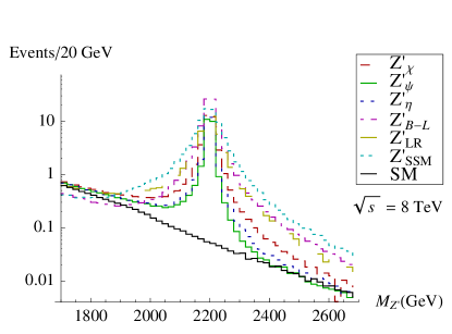
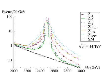
In Fig. 1 we show the shape of the dilepton mass spectrum for a variety of models with TeV at TeV (LHC8), and TeV at TeV (LHC14). The SM background is very small in the resonance mass range, so for luminosities of 20 fb-1 for TeV or 100 fb-1 for TeV, these resonance peaks should be clearly distinguishable. Distributions are calculated at next-to-next-to-leading order. We neglect detector effects such as energy resolution smearing. For ATLAS, the resolution width is about for electrons and for muons Collaboration:2011dca . For CMS, the resolutions widths are for electrons and for muons Timciuc:2011ji . As can be seen in Table 2, the resolutions are generally comparable to or larger than the decay widths for the (assuming that non-SM decay rates are not large). Therefore a precise measurement of the width will likely be difficult Accomando:2010fz . As we show later, there are observables that do not depend strongly on the decay width but still provide useful information about the properties of the .
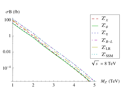
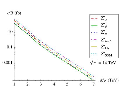
By integrating over the peak region, we can determine the cross section as a function of for each model. In Fig. 2, we show the mass dependence of the integrated peak () cross section for our six model examples at NLO. Note that the mass dependence is largely model-independent.
IV Analysis
We now present a few empirical formulas from our simulations, which allow the cross section and the differential distributions over a wide range of model parameters to be predicted. They are also useful in extracting coupling information from experimental data.
The LHC production cross section of the depends on the mass, width, and couplings. Under the assumption of generational universality, this dependence can be parameterized in the narrow width approximation by
| (7) |
The parameter is model-independent but varies with . It quantifies the fractional contribution to the cross section from up-type quark events. The dependence on the mass is contained in . We use the empirical representation Leike:1998wr ,
| (8) |
of the structure function dependence, where .
As in Refs. Petriello:2008zr ; Carena:2004xs , we define the quantities
| (9) | ||||
| (10) |
In this notation, the cross section formula takes the simple form:
| (11) |
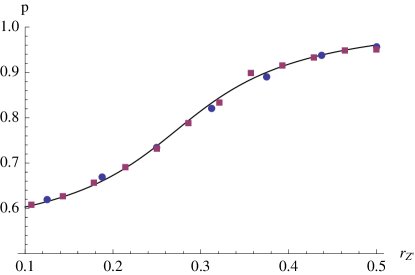
We use a NLO FEWZ simulation of the six model examples in fits of the parameters of Eqs. (7) and (8). First, we fix and fit the simulated cross sections for the six models to the form , then take . We repeat this procedure for several values of over the range, ( TeV for TeV; TeV for TeV), to determine how changes with . We find that this dependence can be approximated by the function
| (12) |
The result is shown in Fig. 3.
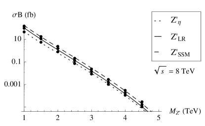
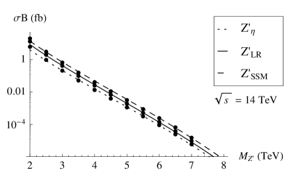
To determine , we fit the normalization to the form given in Eq. (8). Our best fit values are
| (13) |
A comparison of our fit to the simulation is plotted in Fig. 4. This fit captures the dependence on within over the entire range TeV.
After a is detected, the next step will be to measure its couplings. Measuring couplings with precision requires a large number of events, which may not be the situation for a very heavy or weakly coupled . However, with enough events, an accurate measurement of and is possible, as we demonstrate by considering a set of simulated measurements of a 2.5 TeV at TeV.
The coupling combinations and of Eq. (9) can be determined by considering the differential cross section, integrated over the resonance peak:
| (14) | ||||
The functions are normalized so that integrating over and yields Eq. (11). represents the mass dependence of the term, similar to . For TeV, its value is fb. For the same mass, we find fb.
We have already determined , , and , so all that remains is to find . In order to separate the up and down contributions to the differential cross section, we define two distinct scenarios in which the couples exclusively to one type of quark (and to leptons). Then, for each scenario we simulate two differential distributions. The first is the dilepton rapidity distribution, which allows us to determine . To determine , instead of using the total cross section, we consider the quantity , where is the number of lepton pairs scattered in the forward () direction in the Collins-Soper frame PhysRevD.16.2219 and is the number scattered in the backward direction. The resulting distributions are easily distinguishable, as can be seen in Fig. 5. In addition to the simulated NLO data, Fig. 5 shows approximate curves . The specific curves used to approximate the normalized distributions at 14 TeV are
| (15) |


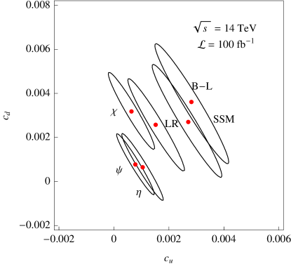
By fitting observed data to Eq. (14), one can determine the four coefficients and . To demonstrate the feasibility of this method and estimate the statistical error, we use our simulation as a pseudo-experiment. For each reference model in Section III, we generate binned distributions for and . To extract and , we fit these distributions to linear combinations of and by minimizing . To determine the boundaries of the confidence regions, we vary and and calculate the value at each point for an “average” experiment using the method described in Appendix A of deGouvea:1999wg .
Figures 6 and 7 show the 95% confidence level (C.L.) regions for our example case of a 2.5 TeV at 14 TeV. We see that 100 fb-1 allows for some model differentiation, while for 1 ab-1 of luminosity the confidence regions are narrow. In the right panel of Fig. 6, the red dashed contour shows the values of and for the models as a function of the mixing angle , from which we can see that some model differentiation should be possible. The tilt of the ellipses arises from the requirement that the up and down quark contributions are summed to give the total cross section, restricting and to lie on a line.
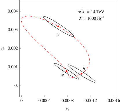
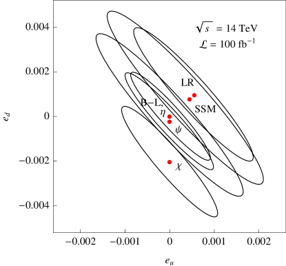
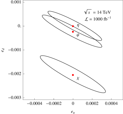
Within the model class, our fit can also be used to place limits on using the least squares method. Using Eqs. (5) and (9), we can write Eq. (14) in terms of instead of and . At the 1-sigma level, we find
| (16) | ||||
If the number of events is low, an analysis can still be done by integrating over the distributions , leading to a system of four equations in four unknowns that can be inverted Petriello:2008zr . Note that we have included only statistical errors. For information on the effect of PDF errors, see Ref. Petriello:2008zr .
From our fit, we can also determine the forward-backward asymmetry,
| (17) |
On the peak, depends solely on the couplings to fermions. Using Eq. (14), integrated over appropriate ranges of , we can write
| (18) |
where . We choose and , the rapidity cuts discussed in Section III.
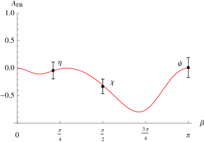
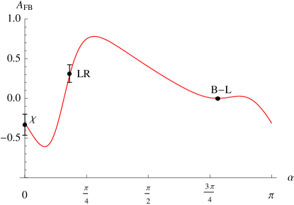
In the left panel of Fig. 8, we show the simulated values of along with statistical uncertainties for three models with 100 fb-1 of data. The red curve shows the predicted values for versus the mixing angle defined in Eq. (5). The couplings of the , , and models can also be parameterized (up to a normalization factor) by an angle with Erler:2011ud
| (19) |
This is equivalent to
| (20) |
where . As for the three models, we show versus in the right panel of Fig 8.
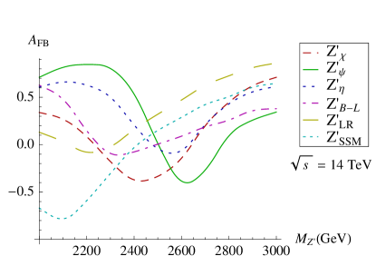
Off peak, the interference with the SM background contributes to the asymmetry, so varies significantly with dilepton mass. Figure 9 shows the effect of this interference on . Both the shape of the curve and the peak value are highly model-dependent.
V Models
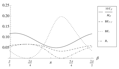
We now consider grand unification scenarios in more detail. An gauge group can be broken down into either a rank-5 or rank-6 subgroup. In the rank-5 case, this leads to one additional boson, the discussed above. In the rank-6 case, there are two additional s, corresponding to the additional and groups in Eq. (III). The mass eigenstates are and of Eq. (5). We justifiably ignore small mixings of the bosons with the SM . Often, the is assumed to be very heavy, leading to an effective rank-5 group, as was the case in the models we considered in Section III. In Fig. 10, we show the branching fractions and total width of each additional boson as a function of the mixing angle .

In the rank-6 case, the masses of the and are related by Barger:1986nn ,
| (21) |
This relation assumes that the symmetry breaking scale is much higher than the electroweak scale. Since the experimental lower bound on the mass is currently about 2 TeV for models, and there are tight limits on mixing with the SM , this is a justified assumption.
Requiring that the be heavier than the , and that both masses are positive leads to the condition
| (22) |
Notice that the , with is excluded from the range in Eq. (22). Additionally, both the and , with and , respectively, have . Therefore, we would not expect the LHC to detect a heavier mass eigenstate for the three models considered in Section III.

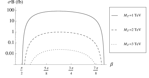
Using the empirical equations determined in Section IV, we can now calculate the cross section for the and . Both cross sections are a function of just two free parameters: and . In Fig. 11, we show the integrated peak cross section for production and decay at LHC14 versus mixing angle. In Fig. 12, we plot the same quantity for the over the allowed range of mixing angles. Here we see that if a were to be discovered in the mass range of TeV or so, the higher mass could be accessible at the LHC as well, within a certain range of mixing angles.
VI Dark Matter Interactions
There are a number of scenarios in which a boson can serve as a dark matter mediator An:2012va ; Buckley:2011mm ; Cline:2011uu ; Petraki:2011mv ; Gondolo:2011eq . These models often include mixing between the gauge bosons, leading to small effective couplings between dark matter and SM fermions Heeck:2011md ; Babu:1997st ; Frandsen:2011cg ; Chun:2010ve ; Cassel:2009pu ; Hook:2010tw ; Mambrini:2010dq . We study this possibility, paying particular attention to the possibility of isospin-violating dark matter scattering, which occurs naturally in the case of a mediator.
We now consider a model with a new and a new Dirac fermion that is charged only under – this fermion will serve as our dark matter candidate. Interactions between the dark matter and SM particles are achieved through the kinetic and mass mixing of the new boson with the SM . The Lagrangian in this case is Babu:1997st
Here and parameterize the kinetic and mass mixing between the and the . As usual, , and are the field strength tensors for , and . are the fermion fields (including the dark matter), and and are the vector and axial charges of the fermions under . For simplicity, we consider the case where all SM fermions have . This choice leads to rather weak couplings between SM fermions and the new , which avoids current LHC bounds on production. must be nonzero to allow for spin-independent scattering of dark matter on nuclei.
We define two additional parameters for convenience:
| (23) | ||||
| (24) |
where is the sine of the weak mixing angle. The couplings to DM and the shifts in the couplings are proportional to . Since is approximately proportional to for , these couplings must be small for heavy s.
The physical states , , and are obtained through two sequential transformations. First, we diagonalize the field strength tensors; then, after breaking, we diagonalize the resulting mass matrices. After these transformations, the physical states are related to the original (hatted) states by
| (25) | ||||
We can write the couplings of the physical states to fermions in terms of the oblique parameters, , , and , and the “physical” weak mixing angle Babu:1997st :
| (26) |
where
| (27) |
and
| (28) |
The contributions to and due to the are, to second order in Babu:1997st ,
| (29) |
| (30) |
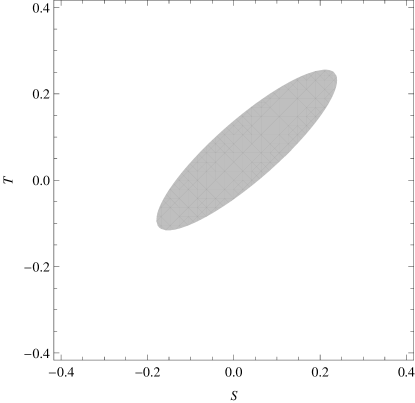
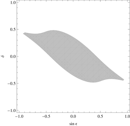
and are constrained by fits to the global electroweak data, as shown in Fig. 13 Nakamura:2010zzi . The best fit values for an assumed Higgs boson mass of GeV are
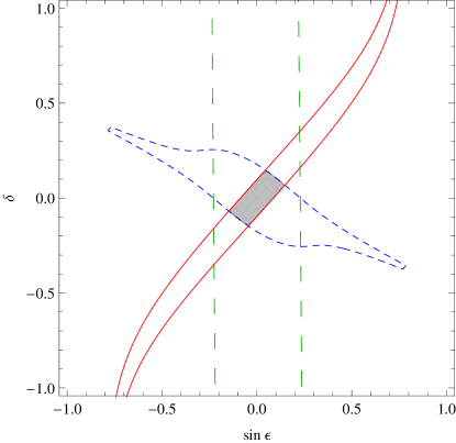
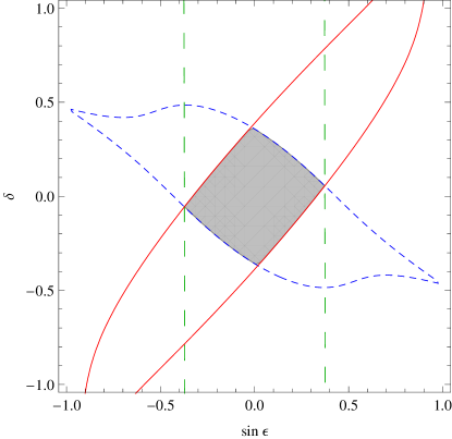
with a strong correlation of . The and values would change very little for a Higgs mass of 125 GeV, as may be suggested by recent LHC observations Chatrchyan:2012tx ; Collaboration:2012si . The constraints on and can be translated into constraints on the mixing angles (and consequently the couplings and cross sections) with a simple Monte Carlo. The result is shown in Fig. 13. Note that the kinetic mixing angle can be quite large, assuming that is small enough.
By sampling values in the region of allowed and , we can determine the range of possible values for the dark matter scattering cross section and the LHC production cross section. These can then be compared to the results of experimental searches to further restrict the mixing angles, mass, and (defined below).
For direct detection experiments, we are interested in interactions between dark matter and atomic nuclei Frandsen:2011cg . To determine this cross section, we start with an effective dark matter-quark coupling given by
| (31) |
which leads to DM-nucleon couplings of
| (32) | ||||
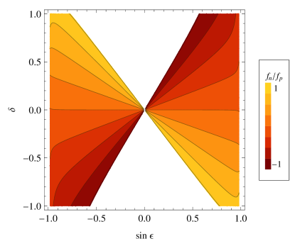
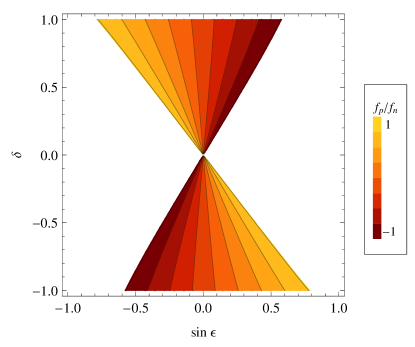
Using these expressions, we can determine as a function of , , and . Contour plots of and as functions of and are shown in Fig. 14. Comparing with Fig. 13, we see that and place no limit on the value of , though the mixing angles are more tightly constrained for some values of than others. Therefore, the limit on the dark matter scattering cross section will vary significantly as a function of .
Finally, we can write the dark matter-nucleus spin-independent scattering cross section:
| (33) |
where is the spin-independent DM-proton cross section,
| (34) |
and and are the atomic and mass numbers of the detector material, is the reduced mass of the dark matter-nucleus system, and is the reduced mass of the dark matter-proton system Feng:2011vu .
It is common to present the spin-independent cross section for a nucleus with Z protons in terms of the cross section for scattering off a single nucleon, making the assumption that . To compare a model with data, we must also account for possible isospin violation. To convert the nuclear cross section to a proton cross section , we multiply by Feng:2011vu
| (35) |
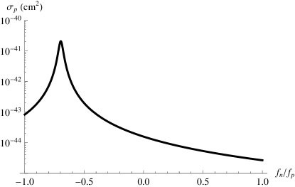
This factor is derived from Eq. (33) by summing over all stable isotopes of atomic number , weighted by their natural abundances . In Fig. 15, we show the effect of isospin violation on the xenon (Z = 54) cross section, normalized to the current limit from XENON100, cm2 at and GeV Aprile:2012nq . Isospin violation can relax the bound by several orders of magnitude, with the least stringent bound occurring around Feng:2011vu .
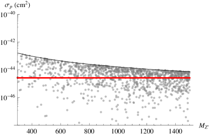
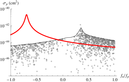
With the XENON bound generalized to all values of , we can use it to place limits on the model parameters. We start by choosing a random sample of points within the allowed region shown in Fig. 13 and then calculate the proton SI cross section for each point. In Figs. 16 and 17, we show the dependence of the cross section on and , respectively. From Fig. 17, we see that the largest cross sections occur for , while the lowest occur for , which is where the XENON bound is the most relaxed. For both figures, we have set and GeV, which in general are free parameters. However, they have no impact on the qualitative features of the distributions, as they only enter the overall normalization factor. They influence our ability to place limits on the other parameters; in particular, the dependence of the cross section means that all constraints can be evaded by choosing a small enough coupling. For GeV and GeV, the XENON bounds are evaded for all values of with .
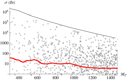
Collider searches can also help constrain the mixing angles for a dark , as the acquires small couplings to SM fermions via mixing effects Frandsen:2012rk . production and decay to leptons at the LHC depends primarily on the mixing angles and the mass, with only a small dependence on the dark matter properties through the decay width of the . Using the couplings in Eq. (VI), we can apply the analysis of Section IV to calculate the cross section for production at the LHC. We find the ATLAS predictions of the cross section for the various models given in Fig. 2 of Ref. Collaboration:2011dca are well parameterized by
| (36) |
With this equation, we can use the current ATLAS limits to restrict the parameter space. Since there are no direct couplings between the and the SM, the lower bound on the mass is much less stringent than for the models considered earlier. In Fig. 18, we show the upper bound on set by the and parameters for TeV.
Finally, we can combine the limits from XENON100 and ATLAS to constrain the model parameter space in terms of , , and . The results are shown in Fig. 19, again with GeV and . The electroweak, dark matter, and LHC data provide complimentary bounds, with and more strongly limiting the degree of mass mixing, while XENON and ATLAS provide more stringent bounds on kinetic mixing. The bounds on and relax as increases and the and decouple. Note that the experiments report their results at different confidence levels, so these regions are not confidence regions; they are simply indicative of the parameter space available.
The invisible decay width of the and the muon anomalous magnetic moment have also been used to constrain the mixing parameters and Chun:2010ve , but they are less restrictive than and for in the range GeV.
If , the invisible decay width of the must be considered. The decay width is proportional to , so the experimental 1.5 MeV bound Nakamura:2010zzi is avoided as long as .
There are also corrections to the muon anomalous magnetic moment Chun:2010ve ,
| (37) |
However, the contributions from the are very small, because of the dependence on and . The current experimental limit is Nakamura:2010zzi , which is several orders of magnitude larger than the expected contribution except for very small .
VII Summary
Our customization of the FEWZ simulation code allows for extensive studies of production and decay at the LHC at NLO and NNLO. Using the results of our simulation for representative benchmark models, we derived an empirical formula for the double differential cross section . This formula can be used to study broad classes of models easily and to determine the couplings to fermions without prior knowledge of the underlying model. In a model-dependent analysis, it can also be used to set limits on model parameters. In the case of the -derived models, without accounting for systematic uncertainties, we find that the mixing angle may be determined within 0.1 with 1 ab-1 of data for a mass of 2.5 TeV. For models we also showed that within a range of mixing angles, two extra neutral gauge bosons should be within the reach of the LHC.
Finally, we considered a more general model with kinetic and mass mixing, which has interesting implications for dark matter detection and hidden sector theories. Even if the SM is uncharged under a new hidden sector , mixing could induce couplings strong enough that the could be produced at the LHC and mediate dark matter scattering on nuclei, without violating limits from global electroweak data. In the case of a heavy () we find that the limits on the and parameters can be combined with XENON100 and LHC data to restrict the range of allowed mixing angles. For a relatively light at 500 GeV, the mass and kinetic mixing parameters and must both be less than about 0.2. For heavy s, these mixing parameters are unrestricted.
Acknowledgments
DM thanks the Galileo Galilei Institute for Theoretical Physics for its hospitality during the completion of this work. This research was supported by the DoE under Grant Nos. DE-FG02-95ER40896 and DE-FG02-04ER41308, by the NSF under Grant No. PHY-0544278, and by the Wisconsin Alumni Research Foundation.
*
Appendix A FEWZ Customization
The FEWZ code allows for an extensive analysis of the SM Drell-Yan process, including NNLO effects and the influence of phase space cuts. With a few modifications, its features can be used to study production as well. The details of the original simulation are provided in Refs. Gavin:2012kw ; Gavin:2010az .
The QCD factorization theorem allows us to write the production cross section in terms of the partonic cross section and the proton structure functions as follows:
Since the addition of a affects only the partonic cross section, and not the structure functions, we do not need to alter the Monte Carlo portion of FEWZ.
The parameters of the model are specified in the input file for each run. For each model, the user sets the mass, total width, partial width to leptons, and couplings of the . The input file also includes the SM parameters and kinematic cuts. We also include a switch to turn on and off the contribution, so that calculations of the SM background can still be done.
The parameters are read into FEWZ and used to calculate “weights” (related to the partonic cross section of various subprocesses) for the integration routine. Preserving the structure of the SM calculation, we insert additional contributions to the partonic cross section. This includes the interference terms mentioned in Eq. (1):
where . Hereafter, the Monte Carlo integration proceeds without alteration.
References
- (1) P. Langacker, “The Physics of Heavy Gauge Bosons,” Rev. Mod. Phys. 81 (2009) 1199–1228, arXiv:0801.1345 [hep-ph].
- (2) M. S. Carena, A. Daleo, B. A. Dobrescu, and T. M. P. Tait, “ gauge bosons at the Tevatron,” Phys. Rev. D70 (2004) 093009, arXiv:hep-ph/0408098.
- (3) A. Leike, “The Phenomenology of extra neutral gauge bosons,” Phys. Rept. 317 (1999) 143–250, arXiv:hep-ph/9805494.
- (4) J. L. Hewett and T. G. Rizzo, “Low-Energy Phenomenology of Superstring Inspired E(6) Models,” Phys. Rept. 183 (1989) 193.
- (5) D. London and J. L. Rosner, “Extra Gauge Bosons in ,” Phys.Rev. D34 (1986) 1530.
- (6) M. T. Frandsen, F. Kahlhoefer, S. Sarkar, and K. Schmidt-Hoberg, “Direct detection of dark matter in models with a light ,” JHEP 09 (2011) 128, arXiv:1107.2118 [hep-ph].
- (7) J. L. Feng, J. Kumar, D. Marfatia, and D. Sanford, “Isospin-Violating Dark Matter,” Phys.Lett. B703 (2011) 124–127, arXiv:1102.4331 [hep-ph].
- (8) R. Gavin, Y. Li, F. Petriello, and S. Quackenbush, “W physics at the LHC with FEWZ 2.1,” arXiv:1201.5896 [hep-ph].
- (9) R. Gavin, Y. Li, F. Petriello, and S. Quackenbush, “FEWZ 2.0: A code for hadronic production at next-to- next-to-leading order,” Comput. Phys. Commun. 182 (2011) 2388–2403, arXiv:1011.3540 [hep-ph].
- (10) CMS Collaboration, S. Chatrchyan et al., “Search for narrow resonances in dilepton mass spectra in pp collisions at sqrt(s) = 7 TeV,” arXiv:1206.1849 [hep-ex].
- (11) ATLAS Collaboration, G. Aad et al., “Search for dilepton resonances in pp collisions at = 7 TeV with the ATLAS detector,” Phys.Rev.Lett. 107 (2011) 272002, arXiv:1108.1582 [hep-ex].
- (12) CMS Collaboration, V. Timciuc, “Search for High-Mass Resonances in the Dilepton Final State with the CMS Detector,” arXiv:1111.4528 [hep-ex].
- (13) XENON100 Collaboration, E. Aprile et al., “Dark Matter Results from 225 Live Days of XENON100 Data,” Phys.Rev.Lett. 109 (2012) 181301, arXiv:1207.5988 [astro-ph.CO].
- (14) J. Erler, P. Langacker, S. Munir, and E. Rojas, “ Bosons at Colliders: a Bayesian Viewpoint,” arXiv:1103.2659 [hep-ph].
- (15) J. Erler, P. Langacker, S. Munir, and E. Rojas, “ Bosons from E(6): Collider and Electroweak Constraints,” arXiv:1108.0685 [hep-ph].
- (16) M. Cvetic and S. Godfrey, “Discovery and identification of extra gauge bosons,” arXiv:hep-ph/9504216 [hep-ph]. Summary of the Working Subgroup on Extra Gauge Bosons of the DPF long-range planning study to be published in Electro-weak Symmetry Breaking and Beyond the Standard Model, eds. T. Barklow, S. Dawson, H. Haber and J. Siegrist (World Scientific 1995).
- (17) T. G. Rizzo, “ phenomenology and the LHC,” arXiv:hep-ph/0610104 [hep-ph].
- (18) F. Petriello and S. Quackenbush, “Measuring couplings at the CERN LHC,” Phys. Rev. D77 (2008) 115004, arXiv:0801.4389 [hep-ph].
- (19) M. Dittmar, A.-S. Nicollerat, and A. Djouadi, “ studies at the LHC: An update,” Phys. Lett. B583 (2004) 111–120, arXiv:hep-ph/0307020.
- (20) CMS Collaboration, S. Chatrchyan et al., “Search for high mass resonances decaying into tau-lepton pairs in pp collisions at sqrt(s) = 7 TeV,” arXiv:1206.1725 [hep-ex].
- (21) E. Accomando, A. Belyaev, L. Fedeli, S. F. King, and C. Shepherd-Themistocleous, “Z’ physics with early LHC data,” Phys.Rev. D83 (2011) 075012, arXiv:1010.6058 [hep-ph].
- (22) C.-F. Chang, K. Cheung, and T.-C. Yuan, “Supersymmetric Decays of the Z’ Boson,” JHEP 1109 (2011) 058, arXiv:1107.1133 [hep-ph].
- (23) V. Barger, T. Han, and D. G. Walker, “Top Quark Pairs at High Invariant Mass: A Model-Independent Discriminator of New Physics at the LHC,” Phys.Rev.Lett. 100 (2008) 031801, arXiv:hep-ph/0612016 [hep-ph].
- (24) F. del Aguila, J. Aguilar-Saavedra, M. Moretti, F. Piccinini, R. Pittau, et al., “Combined analysis of and production for vector resonance searches at LHC,” Phys.Lett. B685 (2010) 302–308, arXiv:0912.3799 [hep-ph].
- (25) D0 Collaboration, V. M. Abazov et al., “Search for a Narrow Resonance in Collisions at TeV,” arXiv:1111.1271 [hep-ex].
- (26) C.-W. Chiang, N. D. Christensen, G.-J. Ding, and T. Han, “Discovery in Drell-Yan Processes at the LHC,” Phys.Rev. D85 (2012) 015023, arXiv:1107.5830 [hep-ph].
- (27) S. Godfrey and T. A. Martin, “Identification of Extra Neutral Gauge Bosons at the LHC Using b- and t-Quarks,” Phys.Rev.Lett. 101 (2008) 151803, arXiv:0807.1080 [hep-ph].
- (28) R. Diener, S. Godfrey, and T. A. Martin, “Discovery and Identification of Extra Neutral Gauge Bosons at the LHC,” arXiv:0910.1334 [hep-ph].
- (29) R. Diener, S. Godfrey, and T. A. Martin, “Unravelling an Extra Neutral Gauge Boson at the LHC using Third Generation Fermions,” Phys.Rev. D83 (2011) 115008, arXiv:1006.2845 [hep-ph].
- (30) O. Eboli, J. Gonzalez-Fraile, and M. Gonzalez-Garcia, “Present Bounds on New Neutral Vector Resonances from Electroweak Gauge Boson Pair Production at the LHC,” arXiv:1112.0316 [hep-ph].
- (31) R. Diener, S. Godfrey, and I. Turan, “Constraining Extra Neutral Gauge Bosons with Atomic Parity Violation Measurements,” arXiv:1111.4566 [hep-ph].
- (32) V. D. Barger and K. Whisnant, “Heavy Z Boson Decays to Two Bosons in E(6) Superstring Models,” Phys.Rev. D36 (1987) 3429.
- (33) V. D. Barger, K. Cheung, and P. Langacker, “Baryonic Z-prime connection of LEP R(b,c) data with Tevatron (W, Z, gamma) b anti-b events,” Phys.Lett. B381 (1996) 226–236, arXiv:hep-ph/9604298 [hep-ph].
- (34) P. Osland, A. Pankov, A. Tsytrinov, and N. Paver, “Spin and model identification of bosons at the LHC,” Phys.Rev. D79 (2009) 115021, arXiv:0904.4857 [hep-ph].
- (35) A. Martin, W. Stirling, R. Thorne, and G. Watt, “Parton distributions for the LHC,” Eur.Phys.J. C63 (2009) 189–285, arXiv:0901.0002 [hep-ph].
- (36) V. Barger, P. Fileviez Perez, and S. Spinner, “Minimal gauged U(1)(B-L) model with spontaneous R-parity violation,” Phys.Rev.Lett. 102 (2009) 181802, arXiv:0812.3661 [hep-ph].
- (37) P. Fileviez Perez and S. Spinner, “The Minimal Theory for R-parity Violation at the LHC,” arXiv:1201.5923 [hep-ph].
- (38) V. Braun, Y.-H. He, B. A. Ovrut, and T. Pantev, “A Heterotic standard model,” Phys.Lett. B618 (2005) 252–258, arXiv:hep-th/0501070 [hep-th].
- (39) B. A. Ovrut, A. Purves, and S. Spinner, “Wilson Lines and a Canonical Basis of SU(4) Heterotic Standard Models,” arXiv:1203.1325 [hep-th].
- (40) L. A. Anchordoqui, I. Antoniadis, H. Goldberg, X. Huang, D. Lust, et al., “LHC Phenomenology and Cosmology of Intersecting D-Brane Models,” arXiv:1206.2537 [hep-ph].
- (41) V. D. Barger, N. Deshpande, and K. Whisnant, “Phenomenology of Electroweak Models with Two Extra Bosons,” Phys.Rev. D35 (1987) 1005.
- (42) R. Mohapatra, Unification and Supersymmetry: The Frontiers of Quark-Lepton Physics. Graduate Texts in Contemporary Physics. Springer-Verlag, 2003. http://books.google.com/books?id=ai12StX-DNoC.
- (43) Particle Data Group Collaboration, K. Nakamura et al., “Review of particle physics,” J. Phys. G37 (2010) 075021.
- (44) J. C. Collins and D. E. Soper, “Angular distribution of dileptons in high-energy hadron collisions,” Phys. Rev. D 16 (Oct, 1977) 2219–2225. http://link.aps.org/doi/10.1103/PhysRevD.16.2219.
- (45) A. de Gouvea, A. Friedland, and H. Murayama, “Seasonal variations of the Be-7 solar neutrino flux,” Phys.Rev. D60 (1999) 093011, arXiv:hep-ph/9904399 [hep-ph].
- (46) H. An, X. Ji, and L.-T. Wang, “Light dark matter and dark force at colliders,” arXiv:1202.2894 [hep-ph].
- (47) M. R. Buckley, D. Hooper, and J. L. Rosner, “A Leptophobic Z’ And Dark Matter From Grand Unification,” Phys.Lett. B703 (2011) 343–347, arXiv:1106.3583 [hep-ph].
- (48) J. M. Cline and A. R. Frey, “Light dark matter versus astrophysical constraints,” Phys.Lett. B706 (2012) 384–388, arXiv:1109.4639 [hep-ph].
- (49) K. Petraki, M. Trodden, and R. R. Volkas, “Visible and dark matter from a first-order phase transition in a baryon-symmetric universe,” arXiv:1111.4786 [hep-ph].
- (50) P. Gondolo, P. Ko, and Y. Omura, “Light dark matter in leptophobic Z’ models,” Phys.Rev. D85 (2012) 035022, arXiv:1106.0885 [hep-ph].
- (51) J. Heeck and W. Rodejohann, “Kinetic and mass mixing with three abelian groups,” Phys.Lett. B705 (2011) 369–374, arXiv:1109.1508 [hep-ph].
- (52) K. S. Babu, C. F. Kolda, and J. March-Russell, “Implications of generalized mixing,” Phys. Rev. D57 (1998) 6788–6792, arXiv:hep-ph/9710441.
- (53) E. J. Chun, J.-C. Park, and S. Scopel, “Dark matter and a new gauge boson through kinetic mixing,” JHEP 02 (2011) 100, arXiv:1011.3300 [hep-ph].
- (54) S. Cassel, D. Ghilencea, and G. Ross, “Electroweak and Dark Matter Constraints on a Z-prime in Models with a Hidden Valley,” Nucl.Phys. B827 (2010) 256–280, arXiv:0903.1118 [hep-ph].
- (55) A. Hook, E. Izaguirre, and J. G. Wacker, “Model Independent Bounds on Kinetic Mixing,” Physical Review Letters (2010) , arXiv:1006.0973 [hep-ph].
- (56) Y. Mambrini, “The Kinetic dark-mixing in the light of CoGENT and XENON100,” JCAP 1009 (2010) 022, arXiv:1006.3318 [hep-ph].
- (57) CMS Collaboration, S. Chatrchyan et al., “Combined results of searches for the standard model Higgs boson in pp collisions at = 7 TeV,” arXiv:1202.1488 [hep-ex].
- (58) ATLAS Collaboration, “Combined search for the Standard Model Higgs boson using up to 4.9 fb-1 of pp collision data at = 7 TeV with the ATLAS detector at the LHC,” arXiv:1202.1408 [hep-ex].
- (59) M. T. Frandsen, F. Kahlhoefer, A. Preston, S. Sarkar, and K. Schmidt-Hoberg, “LHC and Tevatron Bounds on the Dark Matter Direct Detection Cross-Section for Vector Mediators,” JHEP 1207 (2012) 123, arXiv:1204.3839 [hep-ph].