Fluctuation theorems and inequalities generalizing the second law of thermodynamics off equilibrium

Abstract

We present a general framework for systems which are prepared in a non-stationary non-equilibrium state in the absence of any perturbation, and which are then further driven through the application of a time-dependent perturbation. We distinguish two different situations depending on the way the non-equilibrium state is prepared, either it is created by some driving; or it results from a relaxation following some initial non-stationary conditions. Our approach is based on a recent generalization of the Hatano-Sasa relation for non-stationary probability distributions.

We also investigate whether a form of second law holds for separate parts of the entropy production, in a way similar to the work of M. Esposito et al., Phys. Rev. Lett., 104:090601 (2010), but for a non-stationary reference process instead of a stationary one. We find that although the special structure of the theorems derived in this reference is not recovered in the general case, detailed fluctuation theorems still hold separately for parts of the entropy production in this case. These detailed fluctuation theorems lead to interesting generalizations of the second-law of thermodynamics off equilibrium.

I Introduction

In recent years, a broad number of works summarized under the name of fluctuations theorems, have lead to significant progress in our understanding of the second law of thermodynamics Jarzynski2011_vol2 ; Seifert2012_vol ; Harris2007_vol2007 . A central idea, namely the application of thermodynamics at the level of trajectories, has developed into a field of its own, called stochastic thermodynamics Seifert2012_vol ; Seifert2008_vol64 .

In a similar spirit as the Crooks relation Crooks2000_vol61 , the total entropy production can be expressed as the relative entropy between the probability distributions of trajectories associated with a forward and backward experiment Maes2003_vol110 ; Gaspard2004_vol117a ; Kawai2007_vol98 . As a consequence, the entropy production quantifies the time-symmetry breaking and reversibility which means zero entropy production, only occurs when the forward and backward experiments are undistinguishable. While this statement for the entropy production encompasses the second law after averaging over many trajectories, it also provides additional implications at the trajectory level.

This particular idea has also played a central role in recent developments of the framework of fluctuation relations for systems operating under feedback control Sagawa2010_vol104 . A generalization of the Jarzynski relation Jarzynski1997_vol78 including the transfer of information due to feedback predicted theoretically in this reference has been tested experimentally Toyabe2010_vol6 . With these concepts, it is possible to reinterpret Landauer’s principle linking information and thermodynamics Esposito2011_vol95 , and devise new experiments to test it in a particularly elegant and direct way Berut2012_vol483 . Besides providing new insights into the deep connection between thermodynamics and information, progresses in stochastic thermodynamics make it possible to address optimization problems which should be relevant for many applications Aurell2011_vol106 .

In previous work, we have analyzed some consequences of a generalized Hatano-Sasa relation, in which the stationary distribution entering the original Hatano-Sasa relation Hatano2001_vol86 is replaced by a non-stationary one. In Ref. Verley2011_vol , we have shown that this relation offers a way to construct a modified fluctuation-dissipation theorem valid near an arbitrary non-equilibrium state; and in Verley2012_vol108 , we have also derived from it an interesting generalization of the second law of thermodynamics for non-stationary states. Such generalizations of the second law of thermodynamics and of the fluctuation-dissipation theorem are useful to describe the following situations: (i) the system is driven by at least two control parameters, so even when the driving of interest $h$ is constant in time, the probability distribution remains non-stationary and (ii) the system undergoes a transient regime due to the choice of initial conditions, and before the relaxation of this transient regime is finished, the system is further driven. We note that the second situation is typical of systems with a slow relaxation time, such as aging systems, in which case the system never reaches a stationary state on any reasonable time. Therefore, it seems to us that this framework should be ideally suited to analyze aging systems.

In this paper, we provide a more detailed analysis of the results of Ref. Verley2012_vol108 , and we add some new applications. The first section contains preliminaries on fluctuation theorems. We then discuss a particular point concerning the symmetry property that the initial and final probability distributions should have for a detailed fluctuation theorem for the total entropy production to hold. Although this particular point is known in the literature Harris2007_vol2007 , it has been overlooked in many other works in the field despite its importance, and for this reason it seems to us that it was useful to provided a refreshing view about this somewhat subtle point. In the next section, we discuss extensions of the non-adiabatic and adiabatic entropy productions which were introduced in Ref. Esposito2010_vol104 for the case of a stationary reference process. We find that the special structure of the ”three theorems” derived in this reference is not recovered in the general case of a non-stationary reference process. We interpret this as being due to the contribution of a new time-symmetric contribution in the dynamical action, which takes a form similar to the traffic introduced in Ref. Maes2006_vol96 . We then discuss the second-law like inequalities which follow from the integral fluctuation theorems and which should be applicable to a broad class of non-equilibrium systems. In the last section, we present some illustrative examples of these ideas, using a two state model or a particle in an harmonic potential submitted to Langevin dynamics.

II Fluctuation theorems from general considerations of time-reversal symmetry

II.1 Stochastic modelling and definitions

We consider a system which is assumed to evolve according to a continuous-time Markovian dynamics of a pure jump type Feller1940_vol48 . Let us introduce the transition rate $w_{t}(c,c^{\prime})$ for the rate to jump from a state $c$ to a state $c^{\prime}$ at time $t$. The subscript $t$ in $w_{t}(c,c^{\prime})$ indicates that there are processes which are non-stationary even in the absence of explicit driving. The origin of such processes is arbitrary, they can result from an additional underlying driving, which is different from explicit driving and does not need to be specified. Note that if the system is submitted to an initial quench and a constant driving (explicit or not), the rates are time independent but evolution is still non stationary due to the initial quench. At time $t=0$, an arbitrary explicit driving protocol $h_{t}$ is applied to the system, and we denote by $p_{t}(c,[h_{t}])$ the probability to observe the system in the state $c$ at a time $t$ in the presence of this driving. The evolution of the system for $t>0$ is controlled by the generator $L_{t}^{h_{t}}$, which is defined by

$$L^{h_{t}}_{t}(c^{\prime},c)=w^{h_{t}}_{t}(c^{\prime},c)-\delta(c,c^{\prime})\sum_{c^{\prime\prime}}w^{h_{t}}_{t}(c^{\prime},c^{\prime\prime}),$$ (1)

where $w^{h_{t}}_{t}(c^{\prime},c)$ is a transition rate in the presence of the driving $[h_{t}]$. Then $p_{t}(c,[h_{t}])$ is the solution of

$$\frac{dp_{t}(c,[h_{t}])}{dt}=\sum_{c^{\prime}}p_{t}(c^{\prime},[h_{t}])L^{h_{t}}_{t}(c^{\prime},c).$$ (2)

The notation $p_{t}(c,[h_{t}])$ emphasizes that this probability distribution depends functionally on the whole protocol history $[h_{t}]$ up to time $t$. We assume that at $t=0$ there is no driving, so that $p_{0}(c,[h_{0}])=p_{0}(c)$. We also note that in practice, the driving $[h_{t}]$ may not start immediately at $t=0^{+}$ but may be turned on only later, after a certain time, called the waiting time in the context of aging systems.

We now introduce a different probability distribution denoted $\pi_{t}(c,h)$ which represents the probability to observe the system in the state $c$ at a time $t>0$ in the presence of a constant (time independent) driving $h$. In other words, $\pi_{t}(c,h)$ follows from $p_{t}(c,[h_{t}])$ by freezing the time dependence in the driving $[h_{t}]$. This distribution, which will play a key role in the following, obeys the master equation

$$\left(\frac{\partial\pi_{t}}{\partial t}\right)(c,h)=\sum_{c^{\prime}}\pi_{t}(c^{\prime},h)L_{t}^{h}(c^{\prime},c).$$ (3)

From the fact that $\pi_{t}(c,h)$ and $p_{t}(c,[h_{t}])$ should coincide for a constant protocol, we deduce the initial condition to be $\pi_{0}(c,h_{0})=p_{0}(c)$.

In Ref. Verley2011_vol , we have shown that one can construct with this distribution the following functional

$$\mathcal{Y}[c]=-\int_{0}^{T}\mathrm{d}\tau\dot{h}_{\tau}\partial_{h}\ln\pi_{\tau}(c_{\tau},h_{\tau}),$$ (4)

which has clear similarities with the functionals introduced by Jarzynksi Jarzynski1997_vol78 and Hatano-Sasa Hatano2001_vol86 . We find from the analysis of this paper, that the functional $\mathcal{Y}$ has the interpretation of the driving part in the total entropy production. Using a Feynman-Kac approach, which has also played a central role for the Jarzynski relation Hummer2001_vol98 , we have shown in ref. Verley2011_vol that this functional $\mathcal{Y}$ obeys a generalized Hatano-Sasa relation:

$$\langle\exp\left(-\mathcal{Y}[c]\right)\rangle=1$$ (5)

This relation qualifies for a generalization of the Hatano-Sasa relation because the stationary probability distribution $p_{st}(c,h)$ which enters in the functional $Y[c]=-\int_{0}^{T}\mathrm{d}t\,\dot{h}_{t}\partial_{h}\ln p_{st}(c_{t},h_{t})$ in the standard Hatano-Sasa relation is now replaced by the more general distribution $\pi_{t}(c,h)$. From a linear expansion of this generalized Hatano-Sasa, we have obtained modified fluctuation-dissipation theorems valid near an arbitrary non-equilibrium state Verley2011_vol ; Chetrite2009_vol80 . In the next sections, we derive this generalized Hatano-Sasa relation in a different way and we investigate other consequences not contained in such a linear expansion.

II.2 Path probability distributions and action functional

Let us consider a trajectory $[c]=(c_{0},c_{1},...,c_{N};\tau_{1},..,\tau_{N})$ where the $c_{i}$ are the states which are visited by the system and $\tau_{i}$ are the jumping times to go from $c_{i-1}$ to $c_{i}$. The total time-range of the trajectory is $[0..T]$. We denote $\mathcal{P}[c]$ the probability to observe such a trajectory $[c]$, also called path probability below :

$$\mathcal{P}[c]=p_{0}(c_{0})\left[\prod_{j=1}^{N}\exp\left(-\int_{\tau_{j-1}}^{\tau_{j}}\mathrm{d}\tau\lambda^{h_{\tau}}_{\tau}(c_{j-1})\right)w^{h_{\tau_{j}}}_{\tau_{j}}(c_{j-1},c_{j})\right]\exp\left(-\int_{\tau_{N}}^{T}\mathrm{d}\tau\lambda_{\tau}^{h_{\tau}}(c_{N})\right),$$ (6)

where $\lambda^{h_{\tau}}_{\tau}(c^{\prime})=\sum_{c\neq c^{\prime}}w^{h_{\tau}}_{\tau}(c^{\prime},c)$ represents the escape rate to leave the state $c^{\prime}$, and $p_{0}(c_{0})=p_{0}(c_{0},h_{0})$ represents the probability distribution of the initial condition.

In the following, we consider several ratios of path probabilities of the form:

$$\Delta\mathcal{A}[c]=\ln\frac{\mathcal{P}[c]}{\tilde{\mathcal{P}}[c^{*}]},$$ (7)

where the tilde symbol $(\sim)$ corresponds to a transformation of the original dynamics into a new dynamics. This new dynamics is defined by its own initial condition and by the transformed transition rates denoted by $\tilde{w}$. The $(*)$ denotes a different transformation which acts on the trajectory itself. The transformed trajectory $[c^{*}]=(c_{0}^{*},c_{1}^{*},..,c_{N}^{*};\tau_{1}^{*},..,\tau_{N}^{*})$ results from the application of an involution on the trajectory $[c]$ which we assume to be either the identity ($[c^{*}]=[c]$) or the time-reversal symmetry acting on the trajectories ($[c^{*}]=[\bar{c}]=(c_{N},c_{N-1},..,c_{0};T-\tau_{N},..,T-\tau_{1})$). In other words, we have

$$c^{*}_{i}=\left\{\begin{array}[]{ll}c_{i}&\mbox{if $*$ is identity,}\\ c_{N-i}&\mbox{if $*$ is time reversal,}\end{array}\right.\qquad\tau^{*}_{i}=\left\{\begin{array}[]{ll}\tau_{i}&\mbox{if $*$ is identity,}\\ \tau_{N-i+1}&\mbox{if $*$ is time reversal,}\end{array}\right.$$ (8)

with the convention that $\tau^{*}_{0}$ and $\tau^{*}_{N+1}$ are respectively $0$ and $T$ when $*$ is identity and are respectively $T$ and $0$ when $*$ is the time reversal symmetry. Substituting the trajectory $[c^{*}]$ in replacement of $[c]$, and the rates of the modified dynamics $\tilde{w}$ instead of the original rates $w$ in Eq. 6, one obtains directly for the transformed path probability :

$$\tilde{\mathcal{P}}[c^{*}]=\tilde{p}_{0}(c_{0}^{*})\left[\prod_{j=1}^{N}\exp\left(-\int_{\tau^{*}_{j-1}}^{\tau^{*}_{j}}\mathrm{d}\tau\tilde{\lambda}^{h_{\tau}}_{\tau}(c_{j-1}^{*})\right)\tilde{w}^{h_{\tau_{j}^{*}}}_{\tau_{j}^{*}}(c_{j-1}^{*},c_{j}^{*})\right]\exp\left(-\int_{\tau^{*}_{N}}^{\tau^{*}_{N+1}}\mathrm{d}\tau\tilde{\lambda}_{\tau}^{h_{\tau}}(c_{N}^{*})\right),$$ (9)

where $\tilde{\lambda}^{h_{\tau}}_{\tau}(c^{\prime})=\sum_{c\neq c^{\prime}}\tilde{w}^{h_{\tau}}_{\tau}(c^{\prime},c)$ represents the escape rate to leave the state $c^{\prime}$ in the dynamics modified via the operation tilde. From this we see that $\Delta\mathcal{A}[c]$ can be written as

$$\Delta\mathcal{A}[c]=\ln\frac{p_{0}(c_{0})}{\tilde{p_{0}}(c_{0}^{*})}-\int_{0}^{T}dt[\lambda^{h_{t}}_{t}(c_{t})-\tilde{\overset{*}{\lambda}}\,^{h_{t}}_{t}(c_{t})]+\sum_{j=1}^{N}\ln\frac{w_{\tau_{j}}^{h_{\tau_{j}}}(c_{j-1},c_{j})}{\tilde{w}_{\tau_{j}^{*}}^{h_{\tau_{j}^{*}}}(c_{j-1}^{*},c_{j}^{*})},$$ (10)

with $c_{t}=c_{j}$ if $t\in[\tau_{j},\tau_{j+1}[$ and $\overset{*}{\lambda}\,\!^{h_{t}}_{t}=\lambda^{h_{T-t}}_{T-t}$ (or $\overset{*}{\lambda}\,\!^{h_{t}}_{t}=\lambda^{h_{t}}_{t}$) if the involution $*$ is the time reversal (or respectively if $*$ is identity). Thus, $\Delta\mathcal{A}[c]$ has three different contributions: the first term is a boundary term which only depends on the initial or final configurations, the last term is a bulk term, which depends on the whole trajectory. The second term is related to the notion of traffic Baiesi2009_vol103 , which represents the integral of the escape rate $\lambda_{t}$ evaluated at the actual configuration $c_{t}$ of the system at time $t$. In view of this property, the second term in Eq. 10 represents a difference of traffic between the original dynamics (which corresponds to $\mathcal{P}$) and the transformed dynamics (which corresponds to $\tilde{\mathcal{P}}$).

II.3 Protocol-reversal symmetry and the probability distributions of the initial and final points

Fluctuations theorems can be derived from considerations of symmetry for an arbitrary observable and arbitrary initial and final probability distributions Seifert2005_vol95 . These choices of observables, of initial and final probability distributions determine precisely which fluctuation theorem holds. In this construction, we emphasize that the fluctuation theorem takes a strong form if the initial and final probability distributions are related by a reversal of protocol and a weaker form if not Harris2007_vol2007 . Then, two cases must be considered, either the initial and final path probabilities are not related by the reversal of the protocol and the transformation ($\sim$) is not an involution; or such a symmetry exists and the transformation is an involution. In the following, we discuss both cases separately :

• Let us first assume that $\sim$ is not an involution. This occurs for instance when the initial condition does not satisfy $\tilde{\tilde{p}}_{0}(c)=p_{0}(c)$. Following Ref. Esposito2010_vol104 , we consider

  $$P(\Delta\mathcal{A}[c]=\Delta A) = \sum_{[c]}\delta(\Delta\mathcal{A}-\Delta\mathcal{A}[c])\mathcal{P}[c],$$ (11)

  $$= \exp\left(\Delta\mathcal{A}\right)\sum_{[c]}\delta(\Delta\mathcal{A}-\Delta\mathcal{A}[c])\tilde{\mathcal{P}}[c^{*}],$$ (12)

  $$= \exp\left(\Delta\mathcal{A}\right)\tilde{P}(\Delta\mathcal{A}[c^{*}]=\Delta\mathcal{A}),$$ (13)

  with

  $$\tilde{P}(\Delta\mathcal{A}[c^{*}]=\Delta\mathcal{A})=\sum_{[c]}\delta(\Delta\mathcal{A}-\Delta\mathcal{A}[c^{*}])\tilde{\mathcal{P}}[c].$$ (14)

  With words, $\tilde{P}(\Delta\mathcal{A}[c^{*}]=\Delta\mathcal{A})$ corresponds to the probability to have on a given trajectory $[c^{*}]$, $\Delta\mathcal{A}[c^{*}]$ equal to $\Delta\mathcal{A}$ in the tilde experiment/dynamics. When comparing with the expression of $P(\Delta\mathcal{A}[c]=\Delta A)$, it appears that the same function $\Delta\mathcal{A}$ is evaluated on different trajectories ($[c]$ or $[c^{*}]$), which are themselves generated by different dynamics (the original dynamics or the tilde dynamics). Thus, the probability $\tilde{P}(\Delta\mathcal{A}[c^{*}]=\Delta\mathcal{A})$ cannot be defined in itself, i.e. without reference to the quantity $\Delta\mathcal{A}$ introduced in the original dynamics Harris2007_vol2007 . For this reason, we regard the detailed fluctuation theorem (DFT) of Eq. 13 has a weak version of the theorem.

• Let us then assume that the operation ($\sim$) is an involution acting on the path probabilities, $\tilde{\tilde{\mathcal{P}}}=\mathcal{P}$. This implies that the distribution of initial condition satisfies the condition $\tilde{\tilde{p}}_{0}(c)=p_{0}(c)$ and that the transition rates satisfy $\tilde{\tilde{w}}^{h_{t}}_{t}(c,c^{\prime})=w^{h_{t}}_{t}(c,c^{\prime})$. From these two conditions or equivalently directly from the definition Eq. 7, it follows that:

  $$\Delta\mathcal{A}[c]=-\Delta\tilde{\mathcal{A}}[c^{*}],$$ (15)

  where $\Delta\tilde{\mathcal{A}}[c]=\ln\tilde{\mathcal{P}}[c]/\tilde{\tilde{\mathcal{P}}}[c^{*}]$. With this symmetry property, the fluctuation relation for $\Delta\mathcal{A}$ now takes the form

  $$P(\Delta\mathcal{A}[c]=\Delta A) = \exp\left(\Delta\mathcal{A}\right)\sum_{[c]}\delta(\Delta\mathcal{A}+\Delta\tilde{\mathcal{A}}[c^{*}])\tilde{\mathcal{P}}[c^{*}],$$ (16)

  $$= \exp\left(\Delta\mathcal{A}\right)\tilde{P}(\Delta\tilde{\mathcal{A}}[c]=-\Delta\mathcal{A}),$$ (17)

  with

  $$\tilde{P}(\Delta\tilde{\mathcal{A}}[c]=-\Delta\mathcal{A})=\sum_{[c]}\delta(\Delta\mathcal{A}+\Delta\tilde{\mathcal{A}}[c])\tilde{\mathcal{P}}[c],$$ (18)

  which corresponds with words to the probability to have on a given trajectory $[c]$, $\Delta\tilde{\mathcal{A}}[c]$ equal to $-\Delta\mathcal{A}$ in the tilde experiment/dynamics. As expected one can obtain directly Eq. 18 from Eq. 14 using Eq. 15. The main difference with the previous case where tilde was not an involution is that now, it is not the same function which must be evaluated in the two experiments/dynamics characterized by $P$ (resp. $\tilde{P}$); rather it is two different functions, namely $\Delta\mathcal{A}[c]$ and $\Delta\tilde{\mathcal{A}}[c]$) but they are related because they represent the same physical quantity which takes different form on each experiment/dynamics. This is similar to the Crooks relation Crooks2000_vol61 ; Horowitz2007_vol , where the same physical concept, namely the dissipated work, must be evaluated in the direct and tilde experiment/dynamics (although the precise function which represents this physical concept takes a different form in both cases). The main point is that here unlike in the previous case, the function which must be evaluated is linked to the process (direct or reversed) under consideration. We thus regard Eq. 17 as a strong form of the detailed fluctuation theorem.

As a particular important illustration of this point, we discuss below the detailed fluctuation theorem satisfied by the entropy production. To do so, we consider both involutions introduced above, namely $(*)$ and $(\sim)$, to represent a reversal symmetry, respectively the reversal of trajectories and of protocol, which we both denote with a bar $(-)$. We recall that the effect of this symmetry must be considered separately on the trajectories and on the dynamics. The rates which control the dynamics are transformed as

$$\bar{w}^{h_{\tau}}_{\tau}(c,c^{\prime})=w^{h_{T-\tau}}_{T-\tau}(c,c^{\prime}),$$ (19)

since the order in the visited configurations is not affected by the transformation while the time dependance of the driving is. Therefore, one can think of this transformation as basically a time-reversal of all protocols (the driving $[h_{t}]$ and the other protocols represented by the extra subscript in the rates). Note also that Eq. 19 represents a transformation for the rates which is always an involution unlike the full reversal of the path probabilities which may or may not be an involution depending on the initial conditions. This point is very relevant for the existence of a detailed fluctuation theorem for the entropy production. Indeed, in order to identify $\mathcal{A}$ as entropy production, the initial probability distribution of the reversed process must correspond to the final probability distribution reached by the direct process Seifert2005_vol95 . In other words, one must choose $\bar{p_{0}}(\bar{c_{0}})=p_{T}(c_{T})$ where $p_{T}$ is the solution of the Master equation/Fokker Planck equation at time $T$. From Eq. 10, due to the vanishing of the second term, one obtains the familiar result Maes2003_vol110 ; Seifert2005_vol95 :

$$\Delta S_{tot}[c]=\ln\frac{\mathcal{P}[c]}{\bar{\mathcal{P}}[\bar{c}]}=\Delta S+\sum_{j=1}^{N}\ln\frac{w_{\tau_{j}}^{h_{\tau_{j}}}(c_{j-1},c_{j})}{w_{\tau_{j}}^{h_{\tau_{j}}}(c_{j},c_{j-1})},$$ (20)

where the first term $\Delta S=\ln{p_{0}(c_{0})}-\ln{p_{T}(c_{T})}$ represents the change in system stochastic entropy while the second term represents the change in reservoir entropy $\Delta S_{r}[c]$ along the specified trajectory [c].

In view of the discussion above, it is not obvious that the transformation of the full path probability denoted $(-)$ as defined above is an involution in the particular case of the entropy production. Only when additional assumptions are made, namely that the initial and final probability distributions are related by a reversal of the protocol, can this transformation be an involution. Incidentally, this condition means equivalently that the system stochastic entropy $\Delta S$ is antisymmetric with respect to a reversal of the protocol. When this is the case, one obtains from Eq. 17, the following detailed fluctuation relation

$$\ln\frac{P(\Delta S_{tot}[c]=\Delta S_{tot})}{\bar{P}(\Delta\bar{S}_{tot}[c]=-\Delta S_{tot})}=\Delta S_{tot},$$ (21)

which many authors as Esposito2010_vol104 have denoted using a simplified notation

$$\ln\frac{P(\Delta S_{tot})}{\bar{P}(-\Delta S_{tot})}=\Delta S_{tot}.$$ (22)

Note that this relation takes the form of the Evans and Searles theorem Evans2002_vol51 in the following particular cases: (i) for non-equilibrium stationary processes and (ii) for processes generated by time-symmetric driving protocols with the additional condition that the initial and final conditions are related by the reversal of the protocol.

When $p_{0}(c_{0})$ and $\bar{p_{0}}(\bar{c_{0}})$ are not related by a protocol reversal, the detailed fluctuation theorem for the entropy production only holds in its weak form namely Eq. 13. As explained above, this means that the quantity which enters this detailed fluctuation theorem for the reversed process is not the entropy production of that process.

II.4 Dual dynamics and difference of traffic

We now introduce a new transformation, called a duality transformation, which acts specifically on the dynamics of the process. In the following, this transformation is denoted with a hat ($\wedge$). In analogy with the way this dual transformation has been introduced in the stationary case Esposito2010_vol104 ; Hatano2001_vol86 , we define the dual dynamics from the original dynamics by substituting the original rates $w^{h}_{\tau}(c,c^{\prime})$ by :

$$\hat{w}^{h}_{\tau}(c,c^{\prime})=\frac{w^{h}_{\tau}(c^{\prime},c)\pi_{\tau}(c^{\prime},h)}{\pi_{\tau}(c,h)}.$$ (23)

From this definition, it is not obvious that the duality transformation is an involution although it is indeed the case as we show in appendix A. The basic idea is that this transformation essentially reverses the probability currents defined with respect to $\pi_{t}(c,h)$, and because of this, it follows that this transformation is an involution. The proof also confirms that the dynamics constructed from the dual rates is Markovian. The generator of the dynamics still verify $\sum_{c^{\prime}}\hat{L}_{t}^{h_{t}}(c,c^{\prime})=0$, where we have defined $\hat{L}_{t}^{h_{t}}$ as in Eq. 1 substituting the rates $w_{t}^{h_{t}}$ by the rates $\hat{w}_{t}^{h_{t}}$. The normalisation of the probability distribution is thus conserved in time.

An important property of the probability distribution $\pi_{t}(c,h)$ justifying its use to define the duality transform, is that it is related to the difference between the escape rates of the direct and dual dynamics, because :

$$\hat{\lambda}^{h}_{\tau}(c)-\lambda^{h}_{\tau}(c) = \sum_{c^{\prime}\neq c}\left(\hat{w}^{h}_{\tau}(c,c^{\prime})-w^{h}_{\tau}(c,c^{\prime})\right),$$ (24)

$$= \sum_{c^{\prime}\neq c}\left(\pi^{-1}_{\tau}(c,h)w_{\tau}(c^{\prime},c)\pi_{\tau}(c^{\prime},h)-w^{h}_{\tau}(c,c^{\prime})\right),$$ (25)

$$= \sum_{c^{\prime}}\pi^{-1}_{\tau}(c,h)w_{\tau}(c^{\prime},c)\pi_{\tau}(c^{\prime},h)-\sum_{c^{\prime\prime}}w^{h}_{\tau}(c,c^{\prime\prime}),$$ (26)

$$= \sum_{c^{\prime}}\pi^{-1}_{\tau}(c,h)\left(w_{\tau}(c^{\prime},c)-\delta_{c^{\prime}c}\sum_{c^{\prime\prime}}w^{h}_{\tau}(c^{\prime},c^{\prime\prime})\right)\pi_{\tau}(c^{\prime},h),$$ (27)

$$= \pi^{-1}_{\tau}(c,h)\left(\partial_{\tau}\pi_{\tau}\right)(c,h)=\left(\partial_{\tau}\ln\pi_{\tau}\right)(c,h),$$ (28)

where in the last step we used the evolution equation Eq. 3. We define the difference of traffic between the direct and dual dynamics as

$$\Delta\mathcal{T}[c]=\int_{0}^{T}\mathrm{d}\tau\left(\lambda^{h_{\tau}}_{\tau}(c_{\tau})-\hat{\lambda}^{h_{\tau}}_{\tau}(c_{\tau})\right)=-\int_{0}^{T}\mathrm{d}\tau\left(\partial_{\tau}\ln\pi_{\tau}\right)(c_{\tau},h_{\tau}).$$ (29)

From this last expression, we note that the difference of traffic vanishes when the reference probability $\pi_{t}$ is stationary; and that this quantity is antisymmetric under the duality transformation $\Delta\hat{\mathcal{T}}[c]=-\Delta\mathcal{T}[c]$ but symmetric under the combined action of the reversal of the trajectories and of the full protocol (which we regard as the total-reversal symmetry):

$$\Delta\bar{\mathcal{T}}[\bar{c}] = \int_{0}^{T}d\tau\left(\bar{\lambda}_{\tau}^{h_{\tau}}(\bar{c}_{\tau})-\hat{\bar{\lambda}}_{\tau}^{h_{\tau}}(\bar{c}_{\tau})\right),$$ (30)

$$= \int_{0}^{T}d\tau\left(\lambda_{T-\tau}^{h_{T-\tau}}(c_{T-\tau})-\hat{\lambda}_{T-\tau}^{h_{T-\tau}}(c_{T-\tau})\right),$$ (31)

$$= \Delta\mathcal{T}[c],$$ (32)

In the end, combining the total-reversal symmetry and the duality transform together, we obtain that $\Delta\hat{\bar{\mathcal{T}}}[\bar{c}]=-\Delta\mathcal{T}[c]$.

II.5 Adiabatic and non-adiabatic entropy productions

A system can fall into a non-equilibrium state by two mechanisms: (i) either detailed balance can be broken due for instance to boundary conditions or (ii) the system can be driven. Building on a number of works on steady-state thermodynamics Hatano2001_vol86 ; Oono1998_vol ; Speck2005_vol38 ; Chernyak2006_vola , it was shown in Ref. Esposito2010_vol104 that that these two different ways to put a system in a non-equilibrium state correspond to two separate contributions in the entropy production, called adiabatic for case (i) and non-adiabatic for case (ii). Note that this term ”adiabatic” does not refer to the absence of heat exchange but rather to the fact that this contribution is the only one which remains in the adiabatic limit of very slow driving. In this reference, it was shown that surprisingly both terms can be expressed as logratios of probabilities, which implies that both quantities satisfy separately a detailed fluctuation theorem (DFT). This property is surprising because it is not expected to hold for a general splitting of the entropy production. Indeed it does not hold for instance for the splitting of the entropy production into system entropy and reservoir entropy Seifert2005_vol95 . As a further consequence of these DFTs, both the adiabatic part and the non-adiabatic are positive on average, which means that the second law can be split into these two components.

In this section, we generalize the notions of adiabatic and non-adiabatic entropy productions defined as in Esposito2010_vol104 ; Esposito2007_vol76 for the stationary case, by replacing the stationary distribution by the distribution $\pi_{t}(c,h)$ defined in Eq. 3. We obtain the following splitting

$$\Delta S_{na}[c]=\ln\frac{p_{0}(c_{0})}{p_{T}(c_{T},[h_{T}])}+\sum_{j=1}^{N}\ln\frac{\pi_{\tau_{j}}(c_{j},h_{\tau_{j}})}{\pi_{\tau_{j}}(c_{j-1},h_{\tau_{j}})},$$ (33)

and

$$\Delta S_{a}[c]=\sum_{j=1}^{N}\ln\frac{w_{\tau_{j}}^{h_{\tau_{j}}}(c_{j-1},c_{j})\pi_{\tau_{j}}(c_{j-1},h_{\tau_{j}})}{w_{\tau_{j}}^{h_{\tau_{j}}}(c_{j},c_{j-1})\pi_{\tau_{j}}(c_{j},h_{\tau_{j}})},$$ (34)

so that we still have $\Delta S_{tot}[c]=\Delta S_{na}[c]+\Delta S_{a}[c]$.

We note that the adiabatic entropy production verify $\Delta\bar{S}_{a}[\bar{c}]=-\Delta S_{a}[c]$ which means that it is anti-symmetric with respect to the combination of the protocol-reversal and the time-reversal of the trajectories, transformation that we call the total-reversal. On the other side, the non-adiabatic entropy production is anti-symmetric under the total-reversal, i.e. $\Delta\bar{S}_{na}[\bar{c}]=-\Delta S_{na}[c]$, when the total entropy is (provided the appropriate condition on the initial and final states holds as explained in the previous section). We can also define an excess entropy production $\Delta S_{ex}$ such that $\Delta S_{na}[c]=\Delta S+\Delta S_{ex}[c]$ and $\Delta S_{a}[c]=\Delta S_{r}[c]-\Delta S_{ex}[c]$.

It is natural to ask at this point whether $\Delta S_{na}$ and $\Delta S_{a}$ separately satisfy a DFT. These quantities are not a priori of the form of Eq. 7, except for the particular case studied in Esposito2010_vol104 where the reference is stationary, so $\Delta S_{na}$ and $\Delta S_{a}$ should thus not in general satisfy separately a DFT. We thus loose, with the definition of Eqs. 33-34, the positivity of the mean adiabatic and non adiabatic entropy productions. Despite this, we will see that their joint probability distribution still satisfies a DFT as explained in section III.1.

II.6 Non-adiabatic and adiabatic action functionals

In this section, we show that the difference of traffic $\Delta\mathcal{T}$ introduced above is a key observable which can be used to construct quantities which satisfy a DFT. We start from the two possible decompositions of the entropy production as

$$\mbox{(A) }\quad\Delta S_{tot}[c]=\ln\frac{\mathcal{P}[c]}{\hat{\bar{\mathcal{P}}}[\bar{c}]}+\ln\frac{\hat{\bar{\mathcal{P}}}[\bar{c}]}{\bar{\mathcal{P}}[\bar{c}]}\qquad\mbox{ or \; (B) }\qquad\Delta S_{tot}[c]=\ln\frac{\mathcal{P}[c]}{\hat{\mathcal{P}}[c]}+\ln\frac{\hat{\mathcal{P}}[c]}{\bar{\mathcal{P}}[\bar{c}]}.$$ (35)

We first remark that, contrary to the case of Esposito2010_vol104 where the stationary probability distribution is chosen as a reference, the two decompositions are not equivalent. This is due to the fact that the two terms in the decomposition are not anti-symmetric under total-reversal any more, since they contain a non zero difference of traffic term, defined above:

$$\ln\frac{\hat{\bar{\mathcal{P}}}[\bar{c}]}{\bar{\mathcal{P}}[\bar{c}]}\neq\ln\frac{\mathcal{P}[c]}{\hat{\mathcal{P}}[c]}\qquad\mbox{and}\qquad\ln\frac{\hat{\mathcal{P}}[c]}{\bar{\mathcal{P}}[\bar{c}]}\neq\ln\frac{\mathcal{P}[c]}{\hat{\bar{\mathcal{P}}}[\bar{c}]}.$$

Case A - We first focus on the first term in the r.h.s. of Eq. 35A, which we call the non-adiabatic action $\Delta A_{na}[c]$. Using Eq. 10 with the choice $\tilde{\mathcal{P}}=\hat{\bar{\mathcal{P}}}$ for the path probabilities and $c^{*}=\bar{c}$ for the trajectories, we obtain

$$\Delta A_{na}[c]=\ln\frac{\mathcal{P}[c]}{\hat{\bar{\mathcal{P}}}[\bar{c}]}=\ln\frac{p_{0}(c_{0})}{\hat{\bar{p}}_{0}(\bar{c_{0}})}-\int_{0}^{T}\mathrm{d}\tau\left(\lambda^{h_{\tau}}_{\tau}(c_{\tau})-\hat{\lambda}^{h_{\tau}}_{\tau}(c_{\tau})\right)+\sum_{j=1}^{N}\ln\frac{w^{h_{\tau_{j}}}_{\tau_{j}}(c_{j-1},c_{j})}{\hat{w}^{h_{\tau_{j}}}_{\tau_{j}}(c_{j},c_{j-1})}.$$ (36)

Given the initial condition $\hat{\bar{p}}_{0}(\bar{c_{0}})=p_{T}(c_{T})$ for the dual reversed experiment, the first term in this equation corresponds to what we have denoted before $\Delta S=\ln p_{0}(c_{0})-\ln p_{T}(c_{T})$. Using Eq. 23 and Eq. 33, we obtain

$$\Delta A_{na}[c] = \Delta S+\int_{0}^{T}\mathrm{d}\tau\left(\partial_{\tau}\ln\pi_{\tau}\right)(c_{\tau},h_{\tau})+\sum_{j=1}^{N}\ln\frac{\pi_{\tau_{j}}(c_{j},h_{\tau_{j}})}{\pi_{\tau_{j}}(c_{j-1},h_{\tau_{j}})},$$ (37)

$$= \Delta S_{na}[c]-\Delta\mathcal{T}[c],$$

which corresponds to a decomposition into two terms, where the first term, $\Delta S_{na}[c]$, is anti-symmetric and the second term, $\Delta\mathcal{T}[c]$ symmetric under total-reversal. Alternatively, we can also write the same quantity as

$$\Delta A_{na}[c] = \Delta S+\int_{0}^{T}\mathrm{d}\tau\left(\partial_{\tau}\ln\pi_{\tau}\right)(c_{\tau},h_{\tau})+\sum_{j=1}^{N}\ln\frac{\pi_{\tau_{j}}(c_{j},h_{\tau_{j}})}{\pi_{\tau_{j}}(c_{j-1},h_{\tau_{j}})},$$

$$= \Delta S-\Delta\psi+\int_{0}^{T}d\tau\partial_{\tau}\left(\psi_{\tau}(c_{\tau},h_{\tau})\right)+\int_{0}^{T}\mathrm{d}\tau\left(\partial_{\tau}\ln\pi_{\tau}\right)(c_{\tau},h_{\tau})$$

$$+\sum_{j=1}^{N}\ln\frac{\pi_{\tau_{j}}(c_{j},h_{\tau_{j}})}{\pi_{\tau_{j}}(c_{j-1},h_{\tau_{j}})}$$

$$= \Delta S_{b}+\mathcal{Y}[c],$$ (39)

where $\Delta S_{b}=\Delta S-\Delta\psi$ is a boundary term, with $\Delta\psi=-\ln\pi_{T}(c_{T},h_{T})+\ln\pi_{0}(c_{0},h_{0})$.

Therefore, since $p_{0}(c_{0})=\pi_{0}(c_{0},h_{0})$ by construction,

$$\Delta S_{b}=\ln\frac{\pi_{T}(c_{T},h_{T})}{p_{T}(c_{T})}.$$ (40)

As a result, the average of $\Delta S_{b}$, is related to the Kullback-Leibler divergence between the distributions $\pi_{T}$ and $p_{T}$. Physically, this quantity can be viewed as a measure of the lag between the two distributions, in the same way that one can look at the dissipated work as a measure of the lag between the actual distribution at time $t$ and the corresponding equilibrium distribution with the control parameter at the same value Vaikuntanathan2009_vol87 . When there is no lag, either because $p_{T}$ has relaxed towards $\pi_{T}$, or because the initial probability distribution of the reversed protocol, namely $p_{T}(c_{T})$, is chosen to be $\pi_{T}(c_{T},h_{T})$, then the two distributions are identical and $\Delta S_{b}$ vanishes. In this case, $\Delta A_{na}[c]=\mathcal{Y}[c]$, which satisfies the symmetry condition $\hat{\bar{\mathcal{Y}}}[\bar{c}]=-\mathcal{Y}[c]$. Therefore, from Eq. 7 and Eq. 17, this quantity satisfies a DFT:

$$\ln\frac{P(\mathcal{Y}[c]=\mathcal{Y})}{\hat{\bar{P}}(\hat{\bar{\mathcal{Y}}}[c]=-\mathcal{Y})}=\mathcal{Y}.$$ (41)

If we don’t have a vanishing boundary term, then unfortunately only the weak fluctuation theorem of Eq. 13 is verified

$$\ln\frac{P(\Delta\mathcal{A}[c]=\Delta A_{na})}{\hat{\bar{P}}(\Delta\mathcal{A}[\bar{c}]=\Delta A_{na})}=\Delta A_{na}.$$ (42)

We now look at the second term in Eq. 35A, namely

$$\Delta A_{a}[c]=\Delta S_{tot}[c]-\Delta A_{na}[c]=\ln\frac{\hat{\bar{\mathcal{P}}}[\bar{c}]}{\bar{\mathcal{P}}[\bar{c}]}.$$ (43)

We can rewrite Eq. 43 as

$$\Delta A_{a}[c] = \int_{0}^{T}\mathrm{d}\tau(\lambda^{h_{\tau}}_{\tau}(c_{\tau})-\hat{\lambda}^{h_{\tau}}_{\tau}(c_{\tau}))+\sum_{j=1}^{N}\ln\frac{\hat{\bar{w}}^{h_{T-\tau_{j}}}_{T-\tau_{j}}(c_{j},c_{j-1})}{\bar{w}^{h_{T-\tau_{j}}}_{T-\tau_{j}}(c_{j},c_{j-1})},$$ (44)

$$= -\int_{0}^{T}\mathrm{d}\tau\left(\partial_{\tau}\ln\pi_{\tau}\right)(c_{\tau},h_{\tau})+\sum_{j=1}^{N}\ln\frac{w^{\,h_{\tau_{j}}}_{\tau_{j}}(c_{j-1},c_{j})\pi_{\tau_{j}}(c_{j-1},h_{\tau_{j}})}{w^{\,h_{\tau_{j}}}_{\tau_{j}}(c_{j},c_{j-1})\pi_{\tau_{j}}(c_{j},h_{\tau_{j}})},$$ (45)

$$= \Delta S_{a}[c]+\Delta\mathcal{T}[c],$$ (46)

which corresponds again to a decomposition where the first term, $\Delta S_{a}[c]$, is anti-symmetric and the second term, $\Delta\mathcal{T}[c]$ symmetric under total-reversal. As a self-consistent check, we see that the difference of traffic $\Delta\mathcal{T}$, in $\Delta A_{a}$ exactly compensates an opposite contribution in $\Delta A_{na}$ so that

$$\Delta S_{tot}=\Delta A_{a}+\Delta A_{na}=\Delta S_{na}+\Delta S_{a}.$$ (47)

One important point is to realize that $\Delta A_{a}$ is not of the form of Eq. 7 because it involves a modified path probability both at the numerator and the denominator in its definition. Therefore a detailed fluctuation relation of the form of Eq. 41 is not verified for this quantity.

Case B - One can however find another DFT, by starting from the splitting of the entropy production of Eq. 35B. We define the first term on the r.h.s. by

$$\Delta B_{a}[c]=\ln\frac{\mathcal{P}[c]}{\hat{\mathcal{P}}[c]}=-\Delta\bar{A}_{a}[\bar{c}]=-\Delta\mathcal{T}[c]+\Delta S_{a}[c].$$ (48)

and we also introduce the quantity

$$\Delta B_{na}[c]=\ln\frac{\hat{\mathcal{P}}[c]}{\bar{\mathcal{P}}[\bar{c}]}=\Delta\hat{A}_{na}[c]=\Delta\mathcal{T}[c]+\Delta S_{na}[c].$$ (49)

Here $\Delta B_{a}$ plays a role similar to $\Delta A_{na}$ since it too has the required form to satisfy a detailed FT, which is

$$\ln\frac{P(\Delta B_{a}[c]=\Delta B_{a})}{\hat{P}(\Delta\hat{B}_{a}[c]=-\Delta B_{a})}=\Delta B_{a}.$$ (50)

As before for $\Delta A_{a}$, the remaining part in the total entropy, namely $\Delta B_{na}$, does not satisfy a detailed FT.

II.7 Some limiting cases of interest

In this section, we discuss some of the limiting cases for which the detailed fluctuation relations obtained above simplify. Let us assume that the driving starts at time $t_{di}>0$ and ends at time $t_{df}<T$ for a total duration $t_{d}=t_{df}-t_{di}$.

• When $\pi_{t}(c,h)$ relaxes very quickly to the stationary distribution (on a time scale $\tau_{st}$ such that $\tau_{st}\ll T$ and $\tau_{st}\ll t_{d}$), one recovers from Eq. 33 and Eq. 34 the usual definitions of the non-adiabatic and adiabatic parts of the entropy production. In this case $\Delta\mathcal{T}=0$, and as a result Eq. 41 and Eq. 50 become the usual DFTs satisfied by the non-adiabatic and adiabatic entropies respectively Esposito2010_vol104 .

• In the limit of slow driving $\dot{h}_{t}\simeq 0$, which can happen without having $\pi_{t}(c,h)$ relaxed to a stationary distribution, the driving part of the entropy production, $\mathcal{Y}[c]$, vanishes. Furthermore, the boundary term $\Delta S_{b}$ also vanishes, because in this case $p_{t}(c,[h_{t}])$ relaxes to $\pi_{t}(c,h)$ since $[h_{t}]\rightarrow h$. In this limit $\Delta A_{na}=0$, which justifies a posteriori the name non adiabatic action for $\Delta A_{na}$. The vanishing of $\Delta A_{na}$ has two further consequences, the first one is that Eq. 36 implies $\mathcal{P}[c]=\hat{\bar{\mathcal{P}}}[\bar{c}]$, in other words, the duality and total-reversal compensate each other exactly. Another consequence is that $\Delta A_{a}=\Delta B_{a}=\Delta S_{tot}$, which implies that $\Delta\mathcal{T}=0$ although $\pi_{t}(c,h)$ is time-dependent. Furthermore, the fluctuation theorem of entropy production namely, Eq. 21 coincides with that for $\Delta B_{a}$, namely Eq. 50.

II.8 Modified second law for transition between non-stationary states

The observables introduced in section II.6 verify an integral Fluctuation Theorem and therefore are submitted to second law like inequalities, which are valid for an arbitrary non-equilibrium reference process. This results from the positivity of the Kullback-Leibler divergence between the path probabilities $\mathcal{P}[c]$ and $\hat{\bar{\mathcal{P}}}[\bar{c}]$:

$$D(\mathcal{P}[c]||\hat{\bar{\mathcal{P}}}[\bar{c}])\equiv\sum_{[c]}\mathcal{P}[c]\ln\frac{\mathcal{P}[c]}{\hat{\bar{\mathcal{P}}}[\bar{c}]}=\langle\Delta A_{na}\rangle\geq 0,$$ (51)

and between the distributions $\mathcal{P}[c]$ and $\hat{\mathcal{P}}[c]$

$$D(\mathcal{P}[c]||\hat{\mathcal{P}}[c])=\sum_{[c]}\mathcal{P}[c]\ln\frac{\mathcal{P}[c]}{\hat{\mathcal{P}}[c]}=\langle\Delta B_{a}\rangle\geq 0$$ (52)

In view of Eqs. 37, 48 and 47 , this implies

$$\left\langle\Delta S_{na}\right\rangle\geq\left\langle\Delta\mathcal{T}\right\rangle.$$ (53)

Furthermore, one also has $\left\langle\Delta S_{a}\right\rangle\geq\left\langle\Delta\mathcal{T}\right\rangle$ and $\left\langle\Delta S_{tot}\right\rangle\geq 0$, which taken together imply $\left\langle\Delta S_{tot}\right\rangle\geq\max(2\langle\Delta\mathcal{T}\rangle,0).$ However, all these inequalities are less binding than Eq. 53, because the adiabatic entropy production and the total entropy production are generally increasing function of time whereas the inequality Eq. 53 becomes an equality in the long time limit as explained below. We note furthermore that :

(i) Although we have shown that $\langle\Delta A_{na}\rangle\geq 0$ and $\langle\Delta B_{a}\rangle\geq 0$, the corresponding conjugate quantities of $\Delta A_{na}$ and $\Delta B_{a}$ with respect to the total entropy production, namely $\Delta A_{a}$ and $\Delta B_{na}$, do not have likewise a positive mean in general. That this should be the case can be understood from the consideration of a particular case, namely the case where the initial non-equilibrium condition has been prepared by the application of a protocol, which is exactly compensated by the second protocol (the perturbation) denoted $[h_{t}]$ in this paper. In this case, the system is in equilibrium at all times in the presence of the perturbation. Since the rates satisfy the detailed balance condition, one can check explicitly that this implies $\Delta A_{a}=-\Delta A_{na}$ as expected since the system is in equilibrium and $\Delta S_{tot}=0$. It follows from this that in this case $\langle\Delta A_{a}\rangle\leq 0$ and $\langle\Delta B_{na}\rangle\leq 0$; so in this case $\Delta A_{a}$ and $\Delta B_{na}$ do not have positive means.

(ii) The first inequality in Eq. 53 can be written

$$\langle\mathcal{Y}\rangle\geq D(p_{T}||\pi_{T})\geq 0.$$ (54)

In other words, the average of the functional $\mathcal{Y}$ is bounded by $-\Delta S_{b}=D(p_{T}||\pi_{T})$ which is a measure of the lag between the distributions $p_{T}$ and $\pi_{T}$. As noted before, a similar result holds for the dissipated work for the case of an initial equilibrium probability distribution Vaikuntanathan2009_vol87 . Recalling the definition of the excess entropy, $\Delta S_{na}[c]=\Delta S+\Delta S_{ex}[c]$, one can also express this inequality as a Clausius type inequality of the form

$$\left\langle\Delta S\right\rangle\geq-\left\langle\Delta S_{ex}\right\rangle+\left\langle\Delta\mathcal{T}\right\rangle,$$ (55)

which contains as particular cases, the Clausius form of the second law for transitions between equilibrium states and a modified version of the second law for transitions between NESS Hatano2001_vol86 .

(iii) As noted above, the equality in the first inequality of Eq. 53 holds in the adiabatic limit for infinitely slow driving. In this limit the r.h.s. of Eq. 54 is zero because there is no lag between the distribution $p_{T}$ and $\pi_{T}$. The fact that the inequality can be saturated is essential for identifying Eq. 55 as a generalization of the second law of thermodynamics.

III Fluctuation theorems from consideration of generating functions

Generating functions provide an alternate way to understand fluctuation relations without considering trajectories explicitly. Let us introduce the generating functions of $(\Delta\mathcal{T},\Delta S_{a})$ and of $(\Delta\mathcal{T},\Delta S_{na})$, namely

$$g^{(a)}_{T}(c,\gamma,\epsilon) = \left\langle\delta(c-c_{T})e^{-\gamma\Delta\mathcal{T}[c]-\epsilon\Delta S_{a}[c]}\right\rangle,$$ (56)

$$g^{(na)}_{T}(c,\gamma,\epsilon) = \left\langle\delta(c-c_{T})e^{-\gamma\Delta\mathcal{T}[c]-\epsilon\Delta S_{na}[c]}\right\rangle.$$ (57)

These quantities satisfy deformed master equations of the form :

$$\partial_{t}g^{(a)}_{t}(c,\gamma,\epsilon) = \sum_{c^{\prime}}g^{(a)}_{t}(c^{\prime},\gamma,\epsilon)\left(\frac{w_{t}^{h_{t}}(c,c^{\prime})}{\hat{w}_{t}^{h_{t}}(c,c^{\prime})}\right)^{\epsilon}L_{t}^{h_{t}}(c^{\prime},c)+\gamma(\partial_{t}\ln\pi_{t})(c,h_{t})g^{(a)}_{t}(c,\gamma,\epsilon),$$

$$\partial_{t}g^{(na)}_{t}(c,\gamma,\epsilon) = \sum_{c^{\prime}}g^{(na)}_{t}(c^{\prime},\gamma,\epsilon)\left(\frac{\pi_{t}(c^{\prime},h_{t})p_{t}(c)}{\pi_{t}(c,h_{t})p_{t}(c^{\prime})}\right)^{\epsilon}L_{t}^{h_{t}}(c^{\prime},c)$$ (59)

$$+\left[\gamma(\partial_{t}\ln\pi_{t})(c,h_{t})+\epsilon\partial_{t}\ln p_{t}(c)\right]g^{(na)}_{t}(c,\gamma,\epsilon).$$

We can check that in the special case where $\gamma=-1$ and $\epsilon=1$ the solutions are

$$g^{(a)}_{T}(c,-1,1) = \hat{p}_{T}(c)=\left\langle\delta(c-c_{T})e^{-\Delta B_{a}[c]}\right\rangle,$$ (60)

$$g^{(na)}_{T}(c,-1,1) = p_{T}(c)=\left\langle\delta(c-c_{T})e^{-\Delta A_{na}[c]}\right\rangle$$ (61)

where $\hat{p}_{t}(c)$ is the solution of the master equation with generator $\hat{L}_{t}^{h_{t}}$ as defined in appendix A. Note that Eq 61 can be transformed to remove the boundary term in $\Delta A_{na}[c]$ in the following way

$$p_{T}(c) = \left\langle\delta(c-c_{T})e^{-\Delta S_{b}-\mathcal{Y}[c]}\right\rangle,$$ (62)

$$= \sum_{[c]}\mathcal{P}[c|c_{0}]p_{0}(c_{0})\delta(c-c_{T})\left(\frac{p_{T}(c_{T})\pi_{0}(c_{0},h_{0})}{p_{0}(c_{0})\pi_{T}(c_{T},h_{T})}\right)e^{-\mathcal{Y}[c]},$$ (63)

$$= \frac{p_{T}(c)}{\pi_{T}(c,h_{T})}\sum_{[c]}\mathcal{P}[c]\delta(c-c_{T})e^{-\mathcal{Y}[c]},$$ (64)

so that we finally get the result for the generating function of $\mathcal{Y}[c]$ already obtained in Verley2011_vol :

$$\pi_{T}(c,h_{T})=\left\langle\delta(c-c_{T})e^{-\mathcal{Y}[c]}\right\rangle.$$ (65)

Through integration over $c$, we immediately obtain from Eq. 62, the integrated fluctuation theorem

$$\left\langle e^{-\Delta A_{na}[c]}\right\rangle=1,$$ (66)

given that $\Delta A_{na}=\Delta S_{b}+\mathcal{Y}$. This integrated fluctuation theorem also follows directly from Eq. 42. Similarly, by integrating over $c$ in Eq. 65, we have

$$\left\langle e^{-\mathcal{Y}[c]}\right\rangle=1,$$ (67)

which is nothing but the generalized Hatano-Sasa relation given in Eq. 5. Using the Jensen inequality, we recover from these relations, the second law like inequalities of the previous section.

III.1 Fluctuation theorems for joint probability distributions

As shown in Garcia-Garcia2010_vol82 ; Garcia-Garcia2012_vol2012 , it is possible to derive fluctuation theorems for joint probability distributions of variables which form parts of the total entropy production even when each variable does not satisfy separately a fluctuation theorem. This approach has many advantages as it offers a unifying principle to recover many fluctuation theorems. It is straightforward to apply this idea to the general case of an observable $\Delta\mathcal{A}$ of the form of Eq. 7. We assume that this observable can be decomposed into a sum of $m$ observables which are anti-symmetric with respect to the combined action of the tilde and of the star involutions: $\Delta\mathcal{A}=\sum_{i=1}^{m}\Delta\mathcal{A}_{i}$, with $\Delta\tilde{\mathcal{A}_{i}}[c^{*}]=-\Delta\mathcal{A}_{i}[c]$ for $i=1..m$. We now have

$$P(\Delta\mathcal{A}_{1}[c]=\Delta\mathcal{A}_{1},..,\Delta\mathcal{A}_{m}[c]=\Delta\mathcal{A}_{m}) = \sum_{[c]}\prod_{i=1}^{m}\delta(\Delta\mathcal{A}_{i}-\Delta\mathcal{A}_{i}[c])\mathcal{P}[c],$$

$$= \sum_{[c^{*}]}\prod_{i=1}^{m}\delta(\Delta\mathcal{A}_{i}+\Delta\tilde{\mathcal{A}_{i}}[c^{*}])\exp\left(\Delta\mathcal{A}\right)\tilde{\mathcal{P}}[c^{*}],$$

$$= e^{\Delta\mathcal{A}}\tilde{P}(\Delta\tilde{\mathcal{A}}_{1}[c]=-\Delta\mathcal{A}_{1},..,\Delta\tilde{\mathcal{A}}_{m}[c]=-\Delta\mathcal{A}_{m}).$$

where the probability $\tilde{P}$ is defined by

$$\tilde{P}(\Delta\tilde{\mathcal{A}}_{1}[c]=\Delta\mathcal{A}_{1},..,\Delta\tilde{\mathcal{A}}_{m}[c]=\Delta\mathcal{A}_{m})=\sum_{[c]}\tilde{\mathcal{P}}[c]\prod_{i=1}^{n}\delta(\Delta\mathcal{A}_{i}-\Delta\tilde{\mathcal{A}_{i}}[c]).$$

Note that if the observables $\Delta\mathcal{A}_{i}$ do not satisfy the antisymmetry property with respect to the combined action of the tilde and of the star involutions, we still have a weak form of the fluctuation theorem similar to Eq. 14.

In the particular case of the decomposition of $\Delta S_{tot}$ into $\Delta S_{na}$ and $\Delta S_{a}$ that are anti-symmetric by total reversal, we have

$$\ln\frac{P(\Delta S_{a}[c]=\Delta S_{a},\Delta S_{na}[c]=\Delta S_{na})}{\bar{P}(\Delta\bar{S}_{a}[c]=-\Delta S_{a},\Delta\bar{S}_{na}[c]=-\Delta S_{na})}=\Delta S_{a}+\Delta S_{na}.$$ (69)

We can also apply the same idea on the decomposition $\Delta A_{na}=\Delta S_{na}-\Delta\mathcal{T}$ obtained in Eq. 37. Since, $\Delta S_{na}$ and $\Delta\mathcal{T}$ are both antisymmetric under the combination of the duality and the total-reversal ($\Delta\hat{\bar{S}}_{na}[\bar{c}]=-\Delta S_{na}[c]$ and $\Delta\hat{\bar{\mathcal{T}}}[\bar{c}]=-\Delta\mathcal{T}[c]$), we have

$$\ln\frac{P(\Delta\mathcal{T}[c]=\Delta\mathcal{T},\Delta S_{na}[c]=\Delta S_{na})}{\hat{\bar{P}}(\Delta\hat{\bar{\mathcal{T}}}[c]=-\Delta\mathcal{T},\Delta\hat{\bar{S}}_{na}[c]=-\Delta S_{na})}=\Delta S_{na}-\Delta\mathcal{T}.$$ (70)

In the same way, there is a DFT associated with the decomposition $\Delta B_{a}=\Delta S_{a}-\Delta\mathcal{T}$ because both $\Delta S_{a}$ and $\Delta\mathcal{T}$ are also antisymmetric under the duality transformation ($\Delta\hat{S}_{a}[c]=-\Delta S_{a}[c]$ and $\Delta\hat{\mathcal{T}}[c]=-\Delta\mathcal{T}[c]$). Thus, we have

$$\ln\frac{P(\Delta\mathcal{T}[c]=\Delta\mathcal{T},\Delta S_{a}[c]=\Delta S_{a})}{\hat{P}(\Delta\hat{\mathcal{T}}[c]=-\Delta\mathcal{T},\Delta\hat{S}_{a}[c]=-\Delta S_{a})}=\Delta S_{a}-\Delta\mathcal{T}.$$ (71)

IV Illustrative examples

In the following, we illustrate using simple analytical models, the fluctuation relations and the modified second law discussed above. There are two main ways to create non-stationary reference distributions. Either these non-stationary distributions can be created due to the choice of initial conditions or due to a driving force. We illustrate both cases with a driven two states model, and we focus particularly on the case of sinusoidal driving. Besides this two state model, we also study a model for a particle in an harmonic potential and obeying Langevin dynamics.

IV.1 Two states model dynamics

IV.1.1 Non-stationarity from relaxation due to the initial conditions

We consider a two states model described by the following master equation:

$$\partial_{t}p_{t}(a)=-w^{h_{t}}(a,b)p_{t}(a)+w^{h_{t}}(b,a)p_{t}(b),$$ (72)

where the jump rate from state $a$ to state $b$ is denoted $w^{h_{t}}(a,b)$ in the presence of the driving $h_{t}$, and $w(a,b)$ in the absence of this driving. We arbitrarily parametrize the rates as

$$w^{h_{t}}(a,b)=w(a,b)e^{-h_{t}/2}\qquad\mbox{and}\qquad w^{h_{t}}(b,a)=w(b,a)e^{h_{t}/2},$$ (73)

where $h_{t}$ can be thought of as a force which introduces a biais in the transitions rates. Note also that these rates depend on time only through $h_{t}$. In order to create a non-stationary distribution, we choose the initial probability distribution to be in state $b$, $p_{0}(b)$, at an arbitrary value different from the steady state value ($p_{st}(a)=w(a,b)/(w(a,b)+w(b,a))$). As a result, even in the absence of driving, the system will relax in time.

For simplicity, we assume that the driving follows a half sinusoidal protocol depicted in the inset $(i)$ of figure 1, which implies that both the driving and the transition rates are symmetric with respect to time. In inset $(ii)$ of figure 1, we show the relaxation of $\pi_{t}(b,h)$ towards the equilibrium distribution at a given value of $h$ for two choices of the unperturbed rates. One relaxation is faster than the other one because the unperturbed rates are chosen to be larger.

In order to illustrate the DFT of Eq. 41, we have evaluated numerically the functions $\pi_{t}(c,h)$ for different constant force protocols $h$ with a kinetic Monte Carlo algorithm Gillespie1977_vol173 . Using this data, we have generated an ensemble $\hat{\bar{\mathcal{C}}}$ of trajectories with the dual reversed dynamics. We have also built separately an ensemble $\mathcal{C}$ of trajectories corresponding to the original dynamics. Then, we have measured the probability of $\mathcal{Y}[c]$ with $[c]\in\mathcal{C}$ and the probability of $\hat{\bar{\mathcal{Y}}}_{t}[c]=-\mathcal{Y}[\bar{c}]$ with $[c]\in\hat{\bar{\mathcal{C}}}$ counting the number of times that the value of these functionals were in a given range $[\mathcal{Y},\mathcal{Y}+\delta\mathcal{Y}]$. In figure 1, we verify the detailed fluctuation relation for $\mathcal{Y}$ for the slow and the fast protocol of inset $(i)$. In both cases, the initial condition of the dual reversed experiment was chosen to be $\hat{\bar{p}}_{T}(c)=\pi_{T}(c,h_{T})$ which means that by construction $\Delta S_{b}=0$ and $\Delta A_{na}[c]=\mathcal{Y}[c]$. We find that the probability distributions obtained from these simulations follow the expected symmetry. There is one practical difficulty in these simulations, which is also frequently encountered with other numerical tests of fluctuation theorems. One needs to find conditions such that the system is not too far from equilibrium to get a good overlap between $P(\mathcal{Y})$ and $\hat{\bar{P}}(-\mathcal{Y})$, and at the same time sufficiently out of equilibrium so that the probability distributions are distinct despite numerical errors.

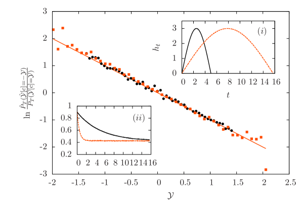
Figure 1: Illustration of the detailed fluctuation relation obeyed by the quantity $\mathcal{Y}$. Orange squares correspond to a long protocol with fast relaxation of the $\pi_{t}$ function towards equilibrium (orange dashed line of the insets) whereas black dots are for a short protocol with slow relaxation towards equilibrium (black solid lines of the insets). Inset $(i)$ shows the half sinusoidal protocols and inset $(ii)$ shows the relaxation, as a function of time $t$, of the distribution $\pi_{t}(b,h)$ towards equilibrium distribution for a given $h$ value.

IV.1.2 Non-stationarity from periodic driving

To illustrate the inequalities generalizing the second-law for transitions between non stationary states obtained in Eq. 53, we use again the same two states model but now with a different protocol. The shape of the protocols for the driving protocol $h_{t}$ and the relaxation of $p_{t}$ towards $\pi_{t}$ is shown in figure 4: the protocol oscillates around an average value $h^{avg}_{t}$ which evolves in time following a piecewise protocol of duration $t_{d}=t_{df}-t_{di}$. This average of the protocol $h^{avg}_{t}$ represents the real driving which induces a transition from one non stationary state to another one, while the oscillations around the average create these non-stationary states. As before, we have used kinetic Monte Carlo simulations to measure the functions $\pi_{t}(a,h^{avg})$ for different values of $h^{avg}$. We have then carried out simulations with the time-dependent driving to obtain the quantities $\left\langle\mathcal{Y}\right\rangle$, $\left\langle\Delta\mathcal{T}\right\rangle$ and $\left\langle\Delta S_{na}\right\rangle$ at fixed final time $T$ for different values of the duration of the driving $t_{d}$. As expected, we observe on figure 2 that $\left\langle\Delta S_{na}\right\rangle\geq\left\langle\Delta\mathcal{T}\right\rangle$. When we calculate $\left\langle\Delta S_{b}\right\rangle$ at the final time $T$, we find a value close to zero irrespective of the duration of the protocol $t_{d}$ because the system has either be driven so slowly that $p_{t}(c,[h])$ has relaxed to $\pi_{t}(c,h_{t})$ already at the end of the protocol at $t_{df}$ or, the system has relaxed afterwards between the times $t_{df}$ and $T$. This is compatible with $\left\langle\mathcal{Y}\right\rangle\geq-\left\langle\Delta S_{b}\right\rangle$, but in fact, since $\left\langle\mathcal{Y}\right\rangle$ does not change between the time $t_{df}$ and $T$, one can obtain a closer bound for $\left\langle\mathcal{Y}\right\rangle$ by evaluating $\left\langle\Delta S_{b}\right\rangle$ at the final time of the driving $t_{df}$ instead of $T$ as shown in figure 2. For this reason, in figure 2, we show $\langle\mathcal{Y}\rangle$, $\langle\Delta S_{na}\rangle$ and $\langle\Delta\mathcal{T}\rangle$ evaluated between the time $t_{di}$ and time $T$ whereas $\left\langle\Delta S_{b}\right\rangle$ is evaluated at time $t_{df}$.

In this figure, we also show that the way $\langle\mathcal{Y}\rangle$ approaches the adiabatic limit for large $t_{d}$ is through a scaling law in $1/t_{d}$. In fact, this is precisely the scaling found in this limit for the dissipated work for a process starting in equilibrium as function of $t_{d}$. This dependence has been first theoretically predicted in Sekimoto1997_vol66 , and recently confirmed in an experiment aimed at testing experimentally the Landauer principle Berut2012_vol483 .

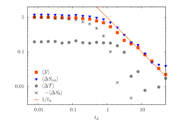
Figure 2: Illustration of the modified second law for non-stationary systems created by periodic driving. Symbols represent the driving entropy production $\langle\mathcal{Y}\rangle$ (filled squares), the non adiabatic entropy production $\langle\Delta S_{na}\rangle$ (filled triangles), the difference of traffic $\langle\Delta\mathcal{T}\rangle$ (bullets) and $\left\langle\Delta S_{b}\right\rangle$ (stars) as function of the duration of the driving $t_{d}$. The solid line is simply $1/t_{d}$ and shows that $\langle\mathcal{Y}\rangle$ and $\langle\Delta S_{na}\rangle$ behave as the inverse of the duration of the driving $t_{d}$ in the limit of large $t_{d}$.

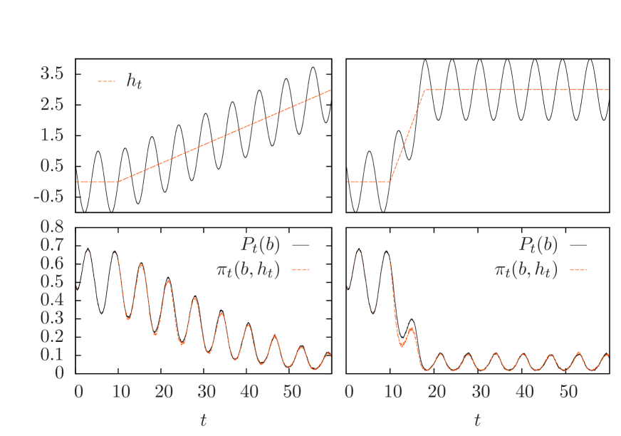
Figure 3: Transition between non stationary oscillating states for different time of driving: (from left to right) $t_{d}=50$ and $t_{d}=7.91$. Top: Protocol imposed in orange dashed lines and in black line the total force applied on the system. Bottom: Exact (black) and accompanying probability distribution (orange) of state $b$ as a function of time. For the shortest protocol, we see that the accompanying distribution is different from the exact solution while the protocol is changing.

IV.2 Overdamped Langevin dynamics

In the previous section, we have used the same control parameter to create the non-stationary state and to induce a transition between the initial and the final non stationary states. On the contrary, in this last section, we consider a particle obeying an overdamped Langevin dynamics in an harmonic potential with two different driving forces, a time-dependent spring constant $k_{t}$ which oscillates and create a non-stationary periodic state, and a piecewise non conservative time dependent force $h_{t}$ which acts as driving inducing transitions. The position $x_{t}$ of the particle is given by the following stochastic differential equation

$$\gamma\dot{x}_{t}=-k_{t}x_{t}+h_{t}+\eta_{t}\sqrt{2\gamma/\beta},$$ (74)

with $\gamma$ the friction coefficient, $\beta$ the inverse temperature and $\eta_{t}$ a Gaussian white noise of mean zero and variance unity. In this case, $x_{t}$ is a gaussian process, which means that the probability distributions $p_{t}(x,[h_{t}])$ and $\pi_{t}(x,h)$ are known from the variance and the average value of the position Verley2011_vol . From these quantities, we obtain $\mathcal{Y}$ directly through Eq. 4 and the boundary term $\Delta S_{b}(t_{df})$ from $\ln\pi_{t_{df}}(x_{t_{df}},h_{t_{df}})-\ln p_{t_{df}}(x_{t_{df}},[h])$. As in the other example, we confirm that $\left\langle\mathcal{Y}\right\rangle\geq-\left\langle\Delta S_{b}\right\rangle$ for all values of the duration of the driving $t_{d}$.

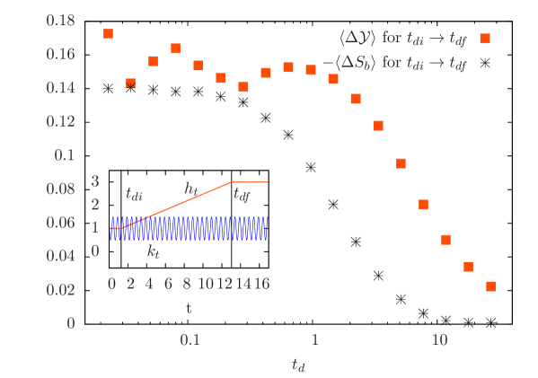
Figure 4: Inset: Transitions between two non stationary states corresponding to the forces $h_{t_{di}}=1.3$ and $h_{t_{df}}=3$. The spring constant is oscillating with a period of $0.5$ around the value $1$ and with an amplitude of $0.5$. The inverse temperature is taken at $\beta=0.2$, the friction is $\gamma=1$.

In a recent experiment, the heat fluctuations of a brownian particle have been measured in an aging gel, created by a sudden temperature quench Gomez-Solano2011_vol106 . This aging gel plays the role of a non-equilibrium bath for the probe particle. With the same experimental setup, the deviation from the fluctuation-theorem has been measured by evaluating separately the correlations and the response function Gomez-SolanoJ.R.2012_vol98 . A complete discussion of these interesting results is out of place here, but instead we show that the detailed fluctuation for the heat exchange obtained in this reference follows from the framework developed in previous sections. The dynamics followed by the probe particule in the experiment is similar to that described by Eq. 74 but differs from it in that in the experiment, there is no driving force and the spring constant is not time dependent. We can adapt the formalism developed in section II.2 to the experimental situation by choosing a similar logratio of probabilities as in Eq. 7 with the tilde operation taken to be the identity, and the star to represent time-reversal. We therefore consider the quantity

$$\Delta\rho[x]=\ln\frac{\mathcal{P}[x]}{\mathcal{P}[\bar{x}]}.$$ (75)

Since the quench, which occurs at time 0, is very fast and there is no subsequent driving in the experiment, the dynamics occurring at time $t>0$ is described by time-independent rates denoted simply $w(c,c^{\prime})$. If we consider now a path probability ratio with trajectories starting at time $t>0$ and finishing at time $T$, we obtain from Eq. 10, that

$$\Delta\rho[x]=\ln\frac{p_{t}(x_{t})}{p_{t}(x_{T})}+\sum_{j\geq j0}^{N}\ln\frac{w(x_{j-1},x_{j})}{w(x_{j},x_{j-1})},$$ (76)

where the index $j_{0}$ corresponds to time $t$. Since tilde was chosen to be the identity, it is obvious that the corresponding transformation of the full path probability is an involution. It follows from section II.2 that in this case

$$\ln\frac{P(\Delta\rho[x]=\Delta\rho)}{P(\Delta\rho[x]=-\Delta\rho)}=\Delta\rho.$$ (77)

Now, the second term in the r.h.s. of Eq. 76 corresponds to what is called medium entropy $\Delta S_{m}$. The temperature of the medium surrounding the probe particle equilibrates very fast (unlike the degrees of freedom associated with the polymers which constitute the gel), so that we can consider that $\Delta S_{m}=-\beta q$, where $\beta=1/T$, and $T$ is the equilibrium temperature of the surrounding medium, with $q$ is the heat exchanged by the particle and the medium. Since there is no work, this heat is simply the variation of internal energy, so $q=k(x_{t+T}^{2}-x_{t}^{2})/2$. Furthermore, since the quench is fast and the system was prepared in an equilibrium state before the quench with a gaussian distribution, the distribution of the initial condition at time $t$ is still a gaussian of variance denoted $\sigma_{x}^{2}(t)$ in Ref. Gomez-Solano2011_vol106 . At time $t+T$, it is assumed that the system is equilibrated so that $k\sigma_{x}^{2}(t+T)=k_{B}T$. In view of this, we obtain from Eq. 77, the fluctuation relation satisfied by the heat $q$ obtained in this reference with $\Delta\rho=-\Delta\beta q$, and

$$\Delta\beta=\frac{k_{B}T}{k}\left[\frac{1}{\sigma_{x}(t+T)^{2}}-\frac{1}{\sigma_{x}(t)^{2}}\right],$$ (78)

which is interpreted as an effective temperature imbalance Gomez-Solano2011_vol106 . This property however only holds for the case of linear Langevin dynamics with a time-independent spring constant.

We thus see on this example that the detailed fluctuation relation satisfied by the heat exchange in Eq. 77 follows from general considerations of a logratio of probabilities of the form of Eq. 75. That this should be the case was also apparent in the derivation of a related fluctuation theorem satisfied by the heat exchange between a system and two thermostats Jarzynski2004_vol92 .

V More complex systems

When using the theoretical framework developed in this paper for complex systems - such as aging systems -, one will encounter the difficulty already present in the standard Hatano-Sasa that the distribution $\pi_{t}(c,h)$ (or $p_{stat}(c,h)$ for the standard Hatano-Sasa) is difficult to determine and may not be a smooth function Perez-Espigares2012_vol85 . Indeed, this distribution can be calculated analytically only in a few simple cases, such as in the case of discrete models involving only a few states or for a particle in an harmonic trap obeying overdamped Langevin dynamics as discussed in the previous section Gomez-Solano2011_vol106 ; Gomez-SolanoJ.R.2012_vol98 . For more complex systems, this distribution will not be accessible analytically. However if the system (or sub-system) of interest is of small size, the numerical determination of this distribution is possible through extensive simulations as we have shown on an example based on the Glauber-Ising model Verley2011_vol . Among the various other strategies which can facilitate this numerical determination, one recent interesting suggestion is to determine the distribution iteratively by starting from an approximate ansatz function Perez-Espigares2012_vol85 .

VI Conclusion

In this paper, we have first emphasized a particular point, namely that a detailed fluctuation theorem can be of strong or weak form depending on whether the initial and final probability distributions have a symmetry under protocol reversal. As we discussed in the case of the entropy production, this property means that the system stochastic entropy is or not anti-symmetric with respect to protocol reversal.

We have then presented a general framework for systems which are prepared in a non-stationary non-equilibrium state in the absence of any perturbation, and which are then further driven through the application of a time-dependent perturbation. Typically for applications, this perturbation is applied as a means to probe the non-equilibrium properties of the unperturbed non-equilibrium state. We can formally distinguish two different situations depending on the way the non-equilibrium state is prepared.

In the first category, the non-equilibrium state is created by some driving, and thus the perturbation which will be applied to it after some time should be viewed as a second driving. As a particular simple example of this category, one can create the initial state by a periodic driving. In these conditions, our approach predicts a modified second law of thermodynamics for transitions between periodically driven states. Such periodically driven states are achievable in a number of experimental systems such as vibrated granular medium, electronic circuits, manipulated colloidal systems, or quantum optics for instance.

In the second category, the initial non-stationary state is a transient state produced by the choice of initial conditions. For instance, the system has been prepared by a quench of some parameter which can be the temperature or the concentration for instance, and the dynamics which follows involves relaxation or coarsening. This is typically what happens in a glassy system, where the slow relaxation following this quench leads to aging.

For all these systems, the generalization of the second law of thermodynamics derived in this paper should hold. In this extension, the dissipated work which enters one form of the standard second law is replaced by the average of a new functional $\langle\mathcal{Y}\rangle$, which can be defined without reference to thermodynamics. We found that this quantity is related to the lag between the actual probability distribution and the $\pi_{t}$ distribution evaluated at the current value of the control parameter, in the same way as the dissipated work is related to the lag with respect to the equilibrium distribution. Furthermore, $\langle\mathcal{Y}\rangle$ approaches the adiabatic limit in a similar way as the dissipated work, ${i.e.}$ in a manner which is proportional to the inverse of the duration of the driving. We hope that our work can contribute to the elaboration of a theoretical framework for modified fluctuation-dissipation theorem and modified second law, in particular for systems in contact with a non-equilibrium bath.

Acknowledgements

We thank U. Seifert, M. Esposito, C. van den Broeck, R. Chétrite and A. Kundu for many insightful discussions in connection with this work.

Appendix A Definition of duality from current reversal

In the main text, we have introduced four dynamics with generators $L_{t}^{h_{t}}$, $\bar{L}_{t}^{h_{t}}$, $\hat{L}_{t}^{h_{t}}$ and $\hat{\bar{L}}_{t}^{h_{t}}$. For all these dynamics, with a generator that we write generally $\tilde{L}_{t}^{h_{t}}$ to encompass all cases, we define a probability distribution $\tilde{p}_{t}(c)$ solution of the following master equation :

$$\frac{d\tilde{p}_{t}(c)}{dt}=\sum_{c^{\prime}}\tilde{p}_{t}(c^{\prime})\tilde{L}^{h_{t}}_{t}(c^{\prime},c).$$ (79)

In the same spirit, we have several reference probability distributions $\pi_{t}(c,h),\bar{\pi}_{t}(c,h),\hat{\pi}_{t}(c,h)$ and $\hat{\bar{\pi}}_{t}(c,h)$ associated to the generators $L_{t}^{h},\bar{L}_{t}^{h},\hat{L}_{t}^{h}$ and $\hat{\bar{L}}_{t}^{h}$, that we note generally $\tilde{\pi}_{t}(c,h)$ with generator $\tilde{L}_{t}^{h}$. The corresponding general master equations is

$$\left(\frac{\partial\tilde{\pi}_{t}}{\partial t}\right)(c,h)=\sum_{c^{\prime}}\tilde{\pi}_{t}(c^{\prime},h)\tilde{L}_{t}^{h}(c^{\prime},c)=\sum_{c^{\prime}}\tilde{\mathcal{J}}_{t}^{h_{t}}(c,c^{\prime}),$$ (80)

in which we have defined the reference probability current of the dynamics modified by the tilde transformation

$$\tilde{\mathcal{J}}^{h}_{t}(c,c^{\prime})=\tilde{\pi}_{t}(c,h)\tilde{w}^{h}_{t}(c,c^{\prime})-\tilde{\pi}_{t}(c^{\prime},h)\tilde{w}^{h}_{t}(c^{\prime},c).$$ (81)

We want to show in this appendix that the dual dynamics corresponds to the dynamics for which accompanying probability currents in the system at time $t$ are opposite to accompanying probability currents in the system with reversed dynamics at time $T-t$, that is to say Crooks2000_vol61 ; Chetrite2008_vol282 :

$$\hat{\mathcal{J}}^{h_{t}}_{t}(c,c^{\prime})=-\bar{\mathcal{J}}^{h_{T-t}}_{T-t}(c,c^{\prime}).$$ (82)

To do so, we start from this definition of duality and find back the dual rates of Eq. 23. First we remark that if all dynamics are connected, it is the same for the reference probability distributions. For instance, we can check that $\hat{\bar{\pi}}_{\tau}(c,h_{\tau})=\pi_{T-\tau}(c,h_{T-\tau})$ by verifying that both quantities are the solution of the same differential equation

$$(\partial_{t}\hat{\pi}_{t})(c^{\prime},h_{t})=\sum_{c}\hat{\mathcal{J}}^{h_{t}}_{t}(c,c^{\prime})=-\sum_{c}\bar{\mathcal{J}}^{h_{T-t}}_{T-t}(c,c^{\prime})=-\left(\partial_{(T-t)}\bar{\pi}_{T-t}\right)(c^{\prime},h_{T-t})$$ (83)

with the same initial condition $\hat{\bar{\pi}}_{0}(c,h_{0})=\pi_{T}(c,h_{T})$. Now, to obtain the dual rates, we use this symmetry $\hat{\pi}_{\tau}(c,h_{\tau})=\bar{\pi}_{T-\tau}(c,h_{T-\tau})$ and Eq 82 to get

$$\hat{\pi}_{t}(c,h_{t})\hat{w}^{h_{t}}_{t}(c,c^{\prime})-\hat{\pi}_{t}(c^{\prime},h_{t})\hat{w}^{h_{t}}_{t}(c^{\prime},c) = -\left(\hat{\pi}_{t}(c,h_{t})\bar{w}^{h_{T-t}}_{T-t}(c,c^{\prime})-\hat{\pi}_{t}(c^{\prime},h_{t})\bar{w}^{h_{T-t}}_{T-t}(c^{\prime},c)\right),$$ (84)

$$= \hat{\pi}_{t}(c^{\prime},h_{t})w^{h_{t}}_{t}(c^{\prime},c)-\hat{\pi}_{t}(c,h_{t})w^{h_{t}}_{t}(c,c^{\prime}).$$

The simplest rates that verify this equality are

$$\hat{w}^{h}_{\tau}(c,c^{\prime})=\frac{w^{h}_{\tau}(c^{\prime},c)\hat{\pi}_{\tau}(c^{\prime},h)}{\hat{\pi}_{\tau}(c,h)}.$$ (85)

The last step consists to use the fact that the duality obtained from Eq. 82 has to be an involution (whereas it was not trivial to see it on Eq 23) in such a way that $\hat{\hat{w}}^{h}_{\tau}(c,c^{\prime})=w^{h}_{\tau}(c,c^{\prime})$. We then end with Eq 23 as another definition of the duality transformation. Note that we have $\bar{\mathcal{J}}^{h_{T-t}}_{T-t}(c,c^{\prime})\neq\mathcal{J}^{h_{t}}_{t}(c,c^{\prime})$ because $\bar{\pi}_{t-T}(c,h_{t-T})\neq\pi_{t}(c,h)$ as we can check using Eq 80 so duality is not a trivial reversal of the current as it was in the stationary reference framework.

References

- [1] Christopher Jarzynski. Equalities and Inequalities: Irreversibility and the Second Law of Thermodynamics at the Nanoscale. 2:329–351, 2011.
- [2] U. Seifert. Stochastic thermodynamics, fluctuation theorems, and molecular machines. ArXiv e-prints, 2012.
- [3] R. J. Harris and G. M. Schütz. Fluctuation theorems for stochastic dynamics. J. Stat. Mech., 2007(07):P07020, 2007.
- [4] U. Seifert. Stochastic thermodynamics: principles and perspectives. Eur. Phys. J. B, 64(3-4):423–431, 2008.
- [5] G. E. Crooks. Path-ensemble averages in systems driven far from equilibrium. Phys. Rev. E, 61(3):2361–2366, 2000.
- [6] C. Maes and K. Netočný. Time-reversal and entropy. J. Stat. Phys., 110(1-2):269–310, 2003.
- [7] P. Gaspard. Time-reversed dynamical entropy and irreversibility in markovian random processes. J. Stat. Phys., 117:599–615, 2004. 10.1007/s10955-004-3455-1.
- [8] R. Kawai, J. M. R. Parrondo, and C. Van den Broeck. Dissipation: The phase-space perspective. Phys. Rev. Lett., 98(8):080602, 2007.
- [9] T. Sagawa and M. Ueda. Generalized Jarzynski equality under nonequilibrium feedback control. Phys. Rev. Lett., 104(9):090602, 2010.
- [10] C. Jarzynski. Nonequilibrium equality for free energy differences. Phys. Rev. Lett., 78(14):2690–2693, 1997.
- [11] S. Toyabe, T. Sagawa, M. Ueda, E. Muneyuki, and M. Sano. Experimental demonstration of information-to-energy conversion and validation of the generalized Jarzynski equality. Nature Physics, 6(12):988–992, 2010.
- [12] M. Esposito and C. Van den Broeck. Second law and landauer principle far from equilibrium. Europhys. Lett., 95(4):40004, 2011.
- [13] A. Berut, A. Arakelyan, A. Petrosyan, S. Ciliberto, R. Dillenschneider, and E. Lutz. Experimental verification of Landauer’s principle linking information and thermodynamics. Nature, 483(7388):187–U1500, 2012.
- [14] E. Aurell, C. Mejía-Monasterio, and P. Muratore-Ginanneschi. Optimal protocols and optimal transport in stochastic thermodynamics. Phys. Rev. Lett., 106:250601–+, 2011.
- [15] T. Hatano and S. I. Sasa. Steady-state thermodynamics of Langevin systems. Phys. Rev. Lett., 86(16):3463–3466, 2001.
- [16] G. Verley, R. Chétrite, and D. Lacoste. Modified fluctuation-dissipation theorem for general non-stationary states and application to the Glauber–Ising chain. J. Stat. Mech., (10):P10025, 2011.
- [17] G. Verley, R. Chétrite, and D. Lacoste. Inequalities generalizing the second law of thermodynamics for transitions between non-stationary states. Phys. Rev. Lett., 108:120601, 2012.
- [18] M. Esposito and C. Van den Broeck. Three detailed fluctuation theorems. Phys. Rev. Lett., 104(9):090601, 2010.
- [19] C. Maes and M. H. van Wieren. Time-symmetric fluctuations in nonequilibrium systems. Phys. Rev. Lett., 96(24):240601, 2006.
- [20] W. Feller. On the integro-differential equations of purely discontinuous Markoff processes. Trans. Am. Math. Soc., 48(3):488–515, 1940.
- [21] G. Hummer and A. Szabo. Free energy reconstruction from nonequilibrium single-molecule pulling experiments. Proc. Natl. Acad. Sci. U.S.A., 98(7):3658–3661, 2001.
- [22] R. Chétrite. Fluctuation relations for diffusion that is thermally driven by a nonstationary bath. Phys. Rev. E, 80(5):051107, 2009.
- [23] M. Baiesi, C. Maes, and B. Wynants. Fluctuations and response of nonequilibrium states. Phys. Rev. Lett., 103:010602, 2009.
- [24] U. Seifert. Entropy production along a stochastic trajectory and an integral fluctuation theorem. Phys. Rev. Lett., 95(4):040602, 2005.
- [25] J. Horowitz and C. Jarzynski. Comparison of work fluctuation relations. J. Stat. Mech., (11):P11002, 2007.
- [26] D.J. Evans and D.J. Searles. The fluctuation theorem. Adv. Phys., 51:1529–1585, 2002.
- [27] Y Oono and M Paniconi. Steady state thermodynamics. Prog. of Theo. Phys. Supplement, (130):29–44, 1998.
- [28] T. Speck and U. Seifert. Integral fluctuation theorem for the housekeeping heat. J. Phys. A: Math. Theor., 38(34):L581–L588, 2005.
- [29] V. Y. Chernyak, M. Chertkov, and C. Jarzynski. Path-integral analysis of fluctuation theorems for general Langevin processes. J. Stat. Mech., page P08001, 2006.
- [30] M. Esposito, U. Harbola, and S. Mukamel. Entropy fluctuation theorems in driven open systems: Application to electron counting statistics. Phys. Rev. E, 76(3):031132, 2007.
- [31] S. Vaikuntanathan and C. Jarzynski. Dissipation and lag in irreversible processes. Europhys. Lett., 87(6):60005, 2009.
- [32] R. García-García, D. Domínguez, V. Lecomte, and A. B. Kolton. Unifying approach for fluctuation theorems from joint probability distributions. Phys. Rev. E, 82(3):030104, 2010.
- [33] R. García-García, V. Lecomte, A. B. Kolton, and D. Domínguez. Joint probability distributions and fluctuation theorems. J. Stat. Mech., 2012(02):P02009, 2012.
- [34] D. T. Gillespie. Exact stochastic simulation of coupled chemical-reactions. Abstracts of Papers of the American Chemical Society, 173:128–128, 1977.
- [35] K. Sekimoto and S.-I. Sasa. Complementarity relation for irreversible process derived from stochastic energetics. Journal of the Physical Society of Japan, 66(11):3326–3328, 1997.
- [36] J. R. Gomez-Solano, A. Petrosyan, and S. Ciliberto. Heat fluctuations in a nonequilibrium bath. Phys. Rev. Lett., 106(20):200602, 2011.
- [37] Gomez-Solano, J. R., Petrosyan, A., and Ciliberto, S. Fluctuations, linear response and heat flux of an aging system. Europhys. Lett., 98(1):10007, 2012.
- [38] C. Jarzynski and D.K. Wójcik. Classical and quantum fluctuation theorems for heat exchange. Phys. Rev. Lett., 92:230602, Jun 2004.
- [39] C. Pérez-Espigares, A. B. Kolton, and J. Kurchan. Infinite family of second-law-like inequalities. Phys. Rev. E, 85:031135, Mar 2012.
- [40] R. Chétrite and K. Gawedzki. Fluctuation relations for diffusion processes. Comm. Math. Phys., 282:469, 2008.