A Course on Derived Categories

0. Introduction

These are notes for an advanced course given at Ben Gurion University in Spring 2012. In this course I am following various sources, mostly [RD], [Sc], [KS2] and [Wei], but going in a sufficiently different route to make written notes desirable. More resources are available on the course web page [CWP].

I want to thank the participants of the course for correcting many of my mistakes, both in real time during the lectures, and in writing. Thanks also to J. Lipman, P. Schapira, A. Neeman and C. Weibel for helpful discussions on the material.

0.1. A motivating discussion: duality

By way of introduction to the subject, let us consider duality. Take a field $K$. Given a $K$-module $M$ (i.e.  a vector space), let

$$D(M):=\operatorname{Hom}_{K}(M,K),$$

be the dual module. There is a canonical homomorphism

$$\eta_{M}:M\to D(D(M)),$$

$\eta_{M}(m)(\phi):=\phi(m)$ for $m\in M$ and $\phi\in D(M)$. If $M$ is finitely generated then $\eta_{M}$ is an isomorphism (actually this is “if and only if”).

To formalize this situation, let $\mathsf{Mod}\,K$ denote the category of $K$-modules. Then

$$D:\mathsf{Mod}\,K\to\mathsf{Mod}\,K$$

is a contravariant functor, and

$$\eta:\boldsymbol{1}\to D\circ D$$

is a natural transformation. Here $\boldsymbol{1}$ is the identity functor of $\mathsf{Mod}\,K$.

Now let us replace $K$ by any (nonzero) commutative ring $A$. Again we can define a contravariant functor

$$D:\mathsf{Mod}\,A\to\mathsf{Mod}\,A,\quad D(M):=\operatorname{Hom}_{A}(M,A),$$

and a natural transformation $\eta:\boldsymbol{1}\to D\circ D$. It is easy to see that $\eta_{M}:M\to D(D(M))$ is an isomorphism if $M$ is a finitely generated free module. Of course we can’t expect reflexivity (i.e. $\eta_{M}$ being an isomorphism) if $M$ is not finitely generated; but what about a finitely generated module that is not free?

In order to understand this better, let us concentrate on the ring $A=\mathbb{Z}$. A finitely generated $\mathbb{Z}$-module $M$, namely a finitely generated abelian group, is of the form $M\cong G\oplus H$, with $G$ free and $H$ finite. It is important to note that this is not a canonical isomorphism: there is a canonical short exact sequence

$$0\to H\to M\to G\to 0,$$

and the decomposition $M\cong G\oplus H$ comes from choosing a splitting of this sequence.

We know that for the free abelian group $G$ there is reflexivity. But for the finite abelian group $H$ we have

$$D(H)=\operatorname{Hom}_{\mathbb{Z}}(H,\mathbb{Z})=0.$$

Thus, whenever $H\neq 0$, reflexivity fails: $\eta_{M}:M\to D(D(M))$ is not an isomorphism.

On the other hand, for an abelian group $M$ we can define another sort of dual:

$$D^{\prime}(M):=\operatorname{Hom}_{\mathbb{Z}}(M,\mathbb{Q}/\mathbb{Z}).$$

(We may view the abelian group $\mathbb{Q}/\mathbb{Z}$ as the group of roots of $1$ in $\mathbb{C}$, via the exponential map.) There is a natural transformation $\eta^{\prime}:\boldsymbol{1}\to D^{\prime}\circ D^{\prime}$, and if $H$ is a finite abelian group then $\eta^{\prime}_{H}$ is an isomorphism. So $D^{\prime}$ is a duality for finite abelian groups. Yet for a finitely generated free abelian group $G$ we get $D^{\prime}(D^{\prime}(G))=\widehat{G}$, the profinite completion of $G$. So once more this is not a good duality for all finitely generated abelian groups.

We could try to be more clever and “patch” the two dualities $D$ and $D^{\prime}$, into something that we will call $D\oplus D^{\prime}$. This looks pleasing at first – but then we recall that the decomposition $M\cong G\oplus H$ of a finitely generated group is not functorial, so that $D\oplus D^{\prime}$ can’t be a functor.

Later in the course we will introduce the derived category $\boldsymbol{\mathsf{D}}(\mathsf{Mod}\,\mathbb{Z})$. The objects of $\boldsymbol{\mathsf{D}}(\mathsf{Mod}\,\mathbb{Z})$ are the complexes of $\mathbb{Z}$-modules. There is a contravariant triangulated functor

$$\mathrm{R}D:\boldsymbol{\mathsf{D}}(\mathsf{Mod}\,\mathbb{Z})\to\boldsymbol{\mathsf{D}}(\mathsf{Mod}\,\mathbb{Z}),$$

$$\mathrm{R}D(M):=\operatorname{RHom}_{\mathbb{Z}}(M,\mathbb{Z}).$$

This is the right derived Hom functor. And there is a natural transformation of triangulated functors

$$\eta:\boldsymbol{1}\to\mathrm{R}D\circ\mathrm{R}D.$$

If $M$ is a bounded complex with finitely generated cohomology modules then $\eta_{M}:M\to\mathrm{R}D(\mathrm{R}D(M))$ is an isomorphism in $\boldsymbol{\mathsf{D}}(\mathsf{Mod}\,\mathbb{Z})$.

We can take a $\mathbb{Z}$-module $M$ and view it as a complex as follows:

(0.1.1) $$\cdots\to 0\to M\to 0\to\cdots$$

where $M$ is in degree $0$. This is a fully faithful embedding of $\mathsf{Mod}\,\mathbb{Z}$ in $\boldsymbol{\mathsf{D}}(\mathsf{Mod}\,\mathbb{Z})$. If $M$ is a finitely generated module then $\eta_{M}$ is an isomorphism. Thus we have a duality $\mathrm{R}D$ that holds for all finitely generated $\mathbb{Z}$-modules!

Here is the connection between $\mathrm{R}D$ and the “classical” dualities $D$ and $D^{\prime}$. Take a finitely generated free abelian group $G$. There is a functorial isomorphism

$$\mathrm{H}^{0}(\mathrm{R}D(G))\cong\operatorname{Hom}_{\mathbb{Z}}(G,\mathbb{Z})=D(G),$$

and $\mathrm{H}^{i}(\mathrm{R}D(G))=0$ for $i\neq 0$. For a finite abelian group $H$ there is a functorial isomorphism

$$\mathrm{H}^{1}(\mathrm{R}D(H))\cong\operatorname{Ext}^{1}_{\mathbb{Z}}(H,\mathbb{Z})\cong D^{\prime}(H),$$

and $\mathrm{H}^{i}(\mathrm{R}D(H))=0$ for $i\neq 1$. Therefore, if $M$ is a finitely generated abelian group, and we choose a decomposition $M\cong G\oplus H$ where $G$ is free and $H$ is finite, there are (noncanonical) isomorphisms

$$\mathrm{H}^{0}(\mathrm{R}D(M))\cong D(G)$$

and

$$\mathrm{H}^{1}(\mathrm{R}D(M))\cong D^{\prime}(H).$$

We see that if $M$ is neither free nor finite, then both $\mathrm{H}^{0}(\mathrm{R}D(M))$ and $\mathrm{H}^{1}(\mathrm{R}D(M))$ are nonzero.

This sort of duality holds for many noetherian commutative rings $A$. But the formula for the duality functor

$$\mathrm{R}D:\boldsymbol{\mathsf{D}}(\mathsf{Mod}\,A)\to\boldsymbol{\mathsf{D}}(\mathsf{Mod}\,A)$$

is somewhat different – it is

$$\mathrm{R}D(M):=\operatorname{RHom}_{A}(M,R),$$

where $R\in\boldsymbol{\mathsf{D}}(\mathsf{Mod}\,A)$ is a dualizing complex. Such a dualizing complex is unique (up to shift and tensoring with an invertible module).

Interestingly, the structure of the dualizing complex $R$ depends on the geometry of the ring $A$ (i.e. of the scheme $\operatorname{Spec}A$). If $A$ is a regular ring (like $\mathbb{Z}$) then $R=A$ is dualizing. If $A$ is Cohen-Macaulay then $R$ is a single $A$-module. But if $A$ is a more complicated ring then $R$ must live in several degrees. For example, consider an affine algebraic variety $X\subset\mathbf{A}^{3}_{\mathbb{R}}$ which is the union of a plane and a line, say with coordinate ring

$$A=\mathbb{R}[t_{1},t_{2},t_{3}]/(t_{3}t_{1},t_{3}t_{2}).$$

See figure 1. The dualizing complex $R$ must live in two adjacent degrees; namely there is some $i$ s.t. $\mathrm{H}^{i}(R)$ and $\mathrm{H}^{i+1}(R)$ are nonzero.

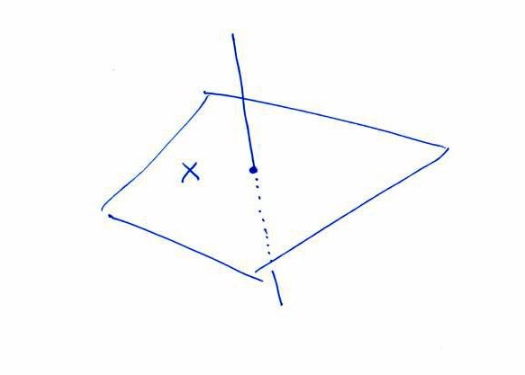
Figure 1.

One can also talk about dualizing complexes over noncommutative rings. I am not sure if we will have time to do that in the course. (But this is a favorite topic for me!)

1. Basics Facts on Categories

1.1. Set Theory

In this course we will not try to be precise about issues of set theory. The blanket assumption is that we are given a Grothendieck universe $\mathsf{U}$. This is an infinite set, closed under most set theoretical operations. A small set (or a $\mathsf{U}$-small set) is a set $S\in\mathsf{U}$. A category $\mathsf{C}$ is a $\mathsf{U}$-category if the set of objects $\operatorname{Ob}(\mathsf{C})$ is a subset of $\mathsf{U}$, and for every $C,D\in\operatorname{Ob}(\mathsf{C})$ the set of morphisms $\operatorname{Hom}_{\mathsf{C}}(C,D)$ is small. See [KS2, Section 1.1]; or see [Ne] for another approach.

We denote by $\mathsf{Set}$ the category of all small sets. So $\operatorname{Ob}(\mathsf{Set})=\mathsf{U}$, and $\mathsf{Set}$ is a $\mathsf{U}$-category. An abelian group (or a ring, etc.) is called small if its underlying set is small. For a small ring $A$ we denote by $\mathsf{Mod}\,A$ the category of all small left $A$-modules.

By default we work with $\mathsf{U}$-categories, and from now on $\mathsf{U}$ will remain implicit. The one exception is when we deal with localization of categories, where we shall briefly encounter a set theoretical issue; but for most interesting cases this issue has an easy solution.

1.2. Zero objects

Let $\mathsf{C}$ be a category. A morphism $f:C\to D$ in $\mathsf{C}$ is called an epimorphism if it has the right cancellation property: for any $g,g^{\prime}:D\to E$, $g\circ f=g^{\prime}\circ f$ implies $g=g^{\prime}$. The morphism $f:C\to D$ is called a monomorphism if it has the left cancellation property: for any $g,g^{\prime}:E\to C$, $f\circ g=f\circ g^{\prime}$ implies $g=g^{\prime}$.

Example 1.2.1.

In $\mathsf{Set}$ the monomorphisms are the injections, and the epimorphisms are the surjections. A morphism $f:C\to D$ in $\mathsf{Set}$ that is both a monomorphism and an epimorphism is an isomorphism. The same holds in $\mathsf{Mod}\,A$.

Remark 1.2.2.

The property of being a monomorphism or an epimorphism is sensitive to the category in question. For instance, consider the category of rings $\mathsf{Ring}$. The forgetful functor $\mathsf{Ring}\to\mathsf{Set}$ respects monomorphisms, but it does not respect epimorphisms. The easiest example is inclusion $\mathbb{Z}\to\mathbb{Q}$, which is an epimorphism in $\mathsf{Ring}$.

By a subobject $C^{\prime}$ of an object $C$ we mean that there is given a monomorphism $f:C^{\prime}\to C$. We sometimes write $C^{\prime}\subset C$ in this situation, but this is only notational (and does not mean inclusion of sets). Likewise, by a quotient $\bar{C}$ of $C$ we mean that there is given an epimorphism $g:C\to\bar{C}$.

An initial object in a category $\mathsf{C}$ is an object $C_{0}\in\mathsf{C}$, such that for every object $C\in\mathsf{C}$ there is exactly one morphism $C_{0}\to C$. Thus the set $\operatorname{Hom}_{\mathsf{C}}(C_{0},C)$ is a singleton. An terminal object in $\mathsf{C}$ is an object $C_{\infty}\in\mathsf{C}$, such that for every object $C\in\mathsf{C}$ there is exactly one morphism $C\to C_{\infty}$.

Definition 1.2.3.

A zero object in a category $\mathsf{C}$ is an object which is both initial and terminal.

Initial, terminal and zero objects are unique up to unique isomorphisms (but they need not exist).

Example 1.2.4.

In $\mathsf{Set}$, $\emptyset$ is an initial object, and any singleton is a terminal object. There is no zero object.

Example 1.2.5.

In $\mathsf{Mod}\,A$, any trivial module (with only the zero element) is a zero object, and we denote this module by $0$. This is allowed, since any other zero module is uniquely isomorphic to it.

1.3. Products and Coproducts

Let $\mathsf{C}$ be a category. For a collection $\{C_{i}\}_{i\in I}$ of objects of $\mathsf{C}$, indexed by a set $I$, their product is a pair $(C,\{p_{i}\}_{i\in I})$ consisting of an object $C$ and morphisms $p_{i}:C\to C_{i}$. The morphisms $p_{i}:C\to C_{i}$ are called projections. The pair $(C,\{p_{i}\}_{i\in I})$ must have this universal property: given any object $D$ and morphisms $f_{i}:D\to C_{i}$, there is a unique morphism $f:D\to C$ s.t. $f_{i}=p_{i}\circ f$. Of course if a product $(C,\{p_{i}\}_{i\in I})$ exists then it is unique up to a unique isomorphism; and we write $\prod_{i\in I}C_{i}:=C$.

Example 1.3.1.

In $\mathsf{Set}$ and $\mathsf{Mod}\,A$ all products (indexed by small sets) exist, and they are the usual cartesian products.

For a collection $\{C_{i}\}_{i\in I}$ of objects of $\mathsf{C}$, their coproduct is a pair $(C,\{e_{i}\}_{i\in I})$ consisting of an object $C$ and morphisms $e_{i}:C_{i}\to C$. The morphisms $e_{i}:C_{i}\to C$ are called embeddings. The pair $(C,\{e_{i}\}_{i\in I})$ must have this universal property: given any object $D$ and morphisms $f_{i}:C_{i}\to D$, there is a unique morphism $f:C\to D$ s.t. $f_{i}=f\circ e_{i}$. If a product $(C,\{e_{i}\}_{i\in I})$ exists then it is unique up to a unique isomorphism; and we write $\coprod_{i\in I}C_{i}:=C$.

Example 1.3.2.

In $\mathsf{Set}$ the coproduct is the disjoint union. In $\mathsf{Mod}\,A$ the coproduct is the direct sum.

1.4. Equivalence

Recall that a functor $F:\mathsf{C}\to\mathsf{D}$ is an equivalence if there exists a functor $G:\mathsf{D}\to\mathsf{C}$, and natural isomorphisms $G\circ F\cong\boldsymbol{1}_{\mathsf{C}}$ and $F\circ G\cong\boldsymbol{1}_{\mathsf{D}}$. Such a functor $G$ is called a quasi-inverse of $F$.

We know that $F:\mathsf{C}\to\mathsf{D}$ is an equivalence iff these two conditions hold:

1. $F$ is essentially surjective on objects. This means that for every $D\in\mathsf{D}$ there is some $C\in\mathsf{C}$ and an isomorphism $F(C)\xrightarrow{\simeq}D$.

2. $F$ is fully faithful. This means that for every $C_{0},C_{1}\in\mathsf{C}$ the function

   $$F:\operatorname{Hom}_{\mathsf{C}}(C_{0},C_{1})\to\operatorname{Hom}_{\mathsf{D}}(F(C_{0}),F(C_{1}))$$

   is bijective.

1.5. Bifunctors

Let $\mathsf{C}$ and $\mathsf{D}$ be categories. Their product is the category $\mathsf{C}\times\mathsf{D}$ defined as follows: the set of objects is

$$\operatorname{Ob}(\mathsf{C}\times\mathsf{D}):=\operatorname{Ob}(\mathsf{C})\times\operatorname{Ob}(\mathsf{D}).$$

The sets of morphisms are

$$\operatorname{Hom}_{\mathsf{C}\times\mathsf{D}}\big{(}(C_{0},D_{0}),(C_{1},D_{1})\big{)}:=\operatorname{Hom}_{\mathsf{C}}(C_{0},C_{1})\times\operatorname{Hom}_{\mathsf{D}}(D_{0},D_{1}).$$

The composition is

$$(\phi_{1},\psi_{1})\circ(\phi_{0},\psi_{0}):=(\phi_{1}\circ\phi_{0},\psi_{1}\circ\psi_{0}),$$

and the identity morphisms are $(1_{C},1_{D})$.

A bifunctor

$$F:\mathsf{C}\times\mathsf{D}\to\mathsf{E}$$

is by definition a functor from the product category $\mathsf{C}\times\mathsf{D}$ to $\mathsf{E}$. We say “bifunctor” because it is a functor of two arguments: $F(C,D)\in\mathsf{E}$.

2. Abelian Categories

2.1. Linear categories

Definition 2.1.1.

Let $\mathbb{K}$ be a commutative ring. A $\mathbb{K}$-linear category is a category $\mathsf{A}$, endowed with a $\mathbb{K}$-module structure on each of the morphism sets $\operatorname{Hom}_{\mathsf{A}}(M_{0},M_{1})$ for all $M_{0},M_{1}\in\mathsf{A}$. The condition is this:

• For all $M_{0},M_{1},M_{2}\in\mathsf{A}$ the composition function

  $$\operatorname{Hom}_{\mathsf{A}}(M_{0},M_{1})\times\operatorname{Hom}_{\mathsf{A}}(M_{1},M_{2})\xrightarrow{\circ}\operatorname{Hom}_{\mathsf{A}}(M_{0},M_{2})$$

  is $\mathbb{K}$-bilinear.

If $\mathbb{K}=\mathbb{Z}$ we say that $\mathsf{A}$ is a linear category.

Observe that for any object $M$ of a $\mathbb{K}$-linear category $\mathsf{A}$, the set

$$\operatorname{End}_{\mathsf{A}}(M):=\operatorname{Hom}_{\mathsf{A}}(M,M)$$

is a $\mathbb{K}$-algebra. In these notes a $\mathbb{K}$-algebra $A$ is (by default) unital and associative; so in fact $A$ is a ring, together with a ring homomorphism from $\mathbb{K}$ to the center of $A$.

This observation can be reversed:

Example 2.1.2.

Let $A$ be a $\mathbb{K}$-algebra. Define a category $\mathsf{A}$ like this: there is a single object $M$, and its set of morphisms is

$$\operatorname{Hom}_{\mathsf{A}}(M,M):=A.$$

Composition in $\mathsf{A}$ is the multiplication of $A$. Then $\mathsf{A}$ is a $\mathbb{K}$-linear category.

2.2. Additive categories

Definition 2.2.1.

An additive category is a linear category $\mathsf{M}$ satisfying these conditions:

• $\mathsf{M}$ has a zero object $0$.

• $\mathsf{M}$ has finite coproducts.

Observe that $\operatorname{Hom}_{\mathsf{M}}(M,N)\neq\emptyset$, since this is an abelian group. Also

$$\operatorname{Hom}_{\mathsf{M}}(M,0)=\operatorname{Hom}_{\mathsf{M}}(0,M)=0,$$

the zero abelian group. We denote the unique arrows $0\to M$ and $M\to 0$ also by $0$. So the numeral $0$ has a lot of meanings; but they are clear from the contexts. The coproduct in the additive category $\mathsf{M}$ is denoted by $\bigoplus$; cf. Example 1.3.2.

Example 2.2.2.

Let $A$ be a ring. The category $\mathsf{Mod}\,A$ is additive. The full subcategory $\mathsf{M}\subset\mathsf{Mod}\,A$ on the free modules is also additive.

for an object $M$ we denote by $1_{M}:M\to M$ the identity morphism.

Proposition 2.2.3.

Let $\mathsf{M}$ be an additive category. Let $\{M_{i}\}_{i\in I}$ be a finite collection of objects of $\mathsf{M}$, and let $M:=\bigoplus_{i\in I}M_{i}$ be the coproduct, with embeddings $e_{i}:M_{i}\to M$.

1. For any $i$ let $p_{i}:M\to M_{i}$ be the unique morphism s.t. $p_{i}\circ e_{i}=1_{M_{i}}$, and $p_{i}\circ e_{j}=0$ for $j\neq i$. Then $(M,\{p_{i}\}_{i\in I})$ is a product of the collection $\{M_{i}\}_{i\in I}$.

2. $\sum_{i\in I}e_{i}\circ p_{i}=1_{M}$.

Proof.

Exercise. ∎

Example 2.2.4.

One could ask if the linear category $\mathsf{A}$ from Example 2.1.2, built from a ring $A$, is additive, i.e. does it have finite direct sums? It appears that this depends on whether or not $A\cong A\oplus A$ as left $A$-modules. Thus if $A$ is nonzero and commutative, or nonzero and noetherian, then this is false. On the other hand if we take a field $\mathbb{K}$, and a countable rank $\mathbb{K}$-module $M$, then $A:=\operatorname{End}_{\mathbb{K}}(M)$ will satisfy $A\cong A\oplus A$.

2.3. Abelian categories

Definition 2.3.1.

Let $\mathsf{M}$ be an additive category, and let $f:M\to N$ be a morphism in $\mathsf{M}$. A kernel of $f$ is a pair $(K,k)$, consisting of an object $K\in\mathsf{M}$ and a morphism $k:K\to M$, with these properties:

1. $f\circ k=0$.

2. If $k^{\prime}:K^{\prime}\to M$ is a morphism in $\mathsf{M}$ such that $f\circ k^{\prime}=0$, then there is a unique morphism $g:K^{\prime}\to K$ such that $k^{\prime}=k\circ g$.

In other words, the object $K$ represents the functor $\mathsf{M}^{\mathrm{op}}\to\mathsf{Ab}$,

$$K^{\prime}\mapsto\{k^{\prime}\in\operatorname{Hom}_{\mathsf{M}}(K^{\prime},M)\mid f\circ k^{\prime}=0\}.$$

The kernel of $f$ is of course unique up to a unique isomorphism (if it exists), and we denote if by $\operatorname{Ker}(f)$. Sometimes $\operatorname{Ker}(f)$ refers only to the object $K$, and other times it refers only to the morphism $k$.

Definition 2.3.2.

Let $\mathsf{M}$ be an additive category, and let $f:M\to N$ be a morphism in $\mathsf{M}$. A cokernel of $f$ is a pair $(C,c)$, consisting of an object $C\in\mathsf{M}$ and a morphism $c:N\to C$, with these properties:

1. $c\circ f=0$.

2. If $c^{\prime}:N\to C^{\prime}$ is a morphism in $\mathsf{M}$ such that $c^{\prime}\circ f=0$, then there is a unique morphism $g:C\to C^{\prime}$ such that $c^{\prime}=g\circ c$.

The cokernel $\operatorname{Coker}(f)$ is unique up to a unique isomorphism.

Example 2.3.3.

In $\mathsf{Mod}\,A$ all kernels and cokernels exist. Given $f:M\to N$, the kernel is $k:K\to M$, where

$$K:=\{m\in M\mid f(m)=0\},$$

and the $k$ is the inclusion. The cokernel is $c:N\to C$, where $C:=N/f(M)$, and $c$ is the canonical projection.

Proposition 2.3.4.

Let $f:M\to N$ be a morphism, let $k:K\to M$ be a kernel of $f$, and let $c:N\to C$ be a cokernel of $f$. Then $k$ is a monomorphism, and $c$ is an epimorphism.

Proof.

Exercise. ∎

Definition 2.3.5.

Assume the additive category $\mathsf{M}$ has kernels and cokernels. Let $f:M\to N$ be a morphism in $\mathsf{M}$.

1. Define the image of $f$ to be

   $$\operatorname{Im}(f):=\operatorname{Ker}(\operatorname{Coker}(f)).$$

2. Define the coimage of $f$ to be

   $$\operatorname{Coim}(f):=\operatorname{Coker}(\operatorname{Ker}(f)).$$

Consider the following commutative diagram (solid arrows):

where $\alpha=\operatorname{Coker}(k)=\operatorname{Coim}(f)$ and $\beta=\operatorname{Ker}(c)=\operatorname{Im}(f)$. Since $c\circ f=0$ there is a unique morphism $\gamma$ making the diagram commutative. Now $\beta\circ\gamma\circ k=f\circ k=0$; and $\beta$ is a monomorphism; so $\gamma\circ k=0$. Hence there is a unique morphism $f^{\prime}:M^{\prime}\to N^{\prime}$ making the diagram commutative. We conclude that $f:M\to N$ induces a morphism

(2.3.6) $$f^{\prime}:\operatorname{Coim}(f)\to\operatorname{Im}(f).$$

Definition 2.3.7.

An abelian category is an additive category $\mathsf{M}$ with these extra properties:

1. All morphisms in $\mathsf{M}$ admit kernels and cokernels.

2. For any $f:M\to N$ in $\mathsf{M}$ the induced morphism $f^{\prime}$ of equation (2.3.6) is an isomorphism.

A less precise but (maybe) easier to remember way to state property (ii) is:

$$\operatorname{Ker}(\operatorname{Coker}(f))=\operatorname{Coker}(\operatorname{Ker}(f)).$$

From now on we forget all about the coimage.

Example 2.3.8.

The category $\mathsf{Mod}\,A$ is abelian.

Definition 2.3.9.

Let $\mathsf{M}$ be an abelian category, and let $\mathsf{N}$ be a full subcategory of $\mathsf{M}$. We say that $\mathsf{N}$ is a full abelian subcategory of $\mathsf{M}$ if $\mathsf{N}$ is closed under direct sums, kernels and cokernels.

Example 2.3.10.

Let $\mathsf{M}_{1}$ be the category of finitely generated abelian groups, and let $\mathsf{M}_{0}$ be the category of finite abelian groups. Then $\mathsf{M}_{0}$ is a full abelian subcategory of $\mathsf{M}_{1}$, and $\mathsf{M}_{1}$ is a full abelian subcategory of $\mathsf{Ab}$.

Example 2.3.11.

Let $\mathsf{N}$ be the full subcategory of $\mathsf{Ab}$ whose objects are the finitely generated free abelian groups. It is an additive subcategory of $\mathsf{Ab}$ (since it is closed under direct sums), but clearly it is not a full abelian subcategory, since it is not closed under cokernels.

What is more interesting is that the additive category $\mathsf{N}$ does have its own intrinsic cokernels, but still it fails to be an abelian category.

Example 2.3.12.

A ring $A$ is left noetherian iff the category $\mathsf{Mod}_{\mathrm{f}}\,A$ of finitely generated modules is a full abelian subcategory of $\mathsf{Mod}\,A$. Here the issue is kernels.

Example 2.3.13.

Let $(X,\mathcal{A})$ be a ringed space; namely $X$ is a topological space and $\mathcal{A}$ is a sheaf of rings on $X$. We denote by $\mathsf{PMod}\,\mathcal{A}$ the category of presheaves of left $\mathcal{A}$-modules on $X$. This is an abelian category. Given a morphism $f:\mathcal{M}\to\mathcal{N}$ in $\mathsf{PMod}\,\mathcal{A}$, its kernel is the presheaf $\mathcal{K}$ defined by

$$\Gamma(U,\mathcal{K}):=\operatorname{Ker}\big{(}f:\Gamma(U,\mathcal{M})\to\Gamma(U,\mathcal{N})\big{)}.$$

The cokernel is the presheaf $\mathcal{C}$ defined by

$$\Gamma(U,\mathcal{C}):=\operatorname{Coker}\big{(}f:\Gamma(U,\mathcal{M})\to\Gamma(U,\mathcal{N})\big{)}.$$

Now let $\mathsf{Mod}\,\mathcal{A}$ be the full subcategory of $\mathsf{PMod}\,\mathcal{A}$ consisting of sheaves. We know that $\mathsf{Mod}\,\mathcal{A}$ is not closed under cokernels inside $\mathsf{PMod}\,\mathcal{A}$, and hence it is not a full abelian subcategory.

However $\mathsf{Mod}\,\mathcal{A}$ is itself an abelian category, but with different cokernels. Indeed, for a morphism $f:\mathcal{M}\to\mathcal{N}$ in $\mathsf{Mod}\,\mathcal{A}$, its cokernel $\operatorname{Coker}_{\mathsf{Mod}\,\mathcal{A}}(f)$ is the sheafification of the presheaf $\operatorname{Coker}_{\mathsf{PMod}\,\mathcal{A}}(f)$.

For educational purposes we state:

Theorem 2.3.14 (Freyd & Mitchell).

Let $\mathsf{M}$ be a small abelian category. Then $\mathsf{M}$ is equivalent to a full abelian subcategory of $\mathsf{Mod}\,A$, for a suitable ring $A$.

This means that most of the time we can pretend that $\mathsf{M}\subset\mathsf{Mod}\,A$; this could be a helpful heuristic.

Proposition 2.3.15.

1. Let $\mathsf{M}$ be an additive category. Then the opposite category $\mathsf{M}^{\mathrm{op}}$ is also additive.

2. Let $\mathsf{M}$ be an abelian category. Then the opposite category $\mathsf{M}^{\mathrm{op}}$ is also abelian.

Proof.

(1) First note that

$$\operatorname{Hom}_{\mathsf{M}^{\mathrm{op}}}(M,N)=\operatorname{Hom}_{\mathsf{M}}(N,M),$$

so this is an abelian group. The bilinearity of the composition in $\mathsf{M}^{\mathrm{op}}$ is clear, and the zero objects are the same. Existence of finite coproducts in $\mathsf{M}^{\mathrm{op}}$ is because of existence of finite products in $\mathsf{M}$; see Proposition 2.2.3(1).

(2) $\mathsf{M}^{\mathrm{op}}$ has kernels and cokernels, since $\operatorname{Ker}_{\mathsf{M}^{\mathrm{op}}}(f)=\operatorname{Coker}_{\mathsf{M}}(f)$ and vice versa. Also the symmetric condition (ii) of Definition 2.3.7 holds. ∎

Proposition 2.3.16.

Let $f:M\to N$ be a morphism in an abelian category $\mathsf{M}$.

1. $f$ is a monomorphism iff $\operatorname{Ker}(f)=0$.

2. $f$ is an epimorphism iff $\operatorname{Coker}(f)=0$.

3. $f$ is an isomorphism iff it is both a monomorphism and an epimorphism.

Proof.

Exercise. ∎

2.4. Additive Functors

Definition 2.4.1.

Let $\mathsf{M}$ and $\mathsf{N}$ be $\mathbb{K}$-linear categories. A functor $F:\mathsf{M}\to\mathsf{N}$ is called a $\mathbb{K}$-linear functor if for every $M_{0},M_{1}\in\mathsf{M}$ the function

$$F:\operatorname{Hom}_{\mathsf{M}}(M_{0},M_{1})\to\operatorname{Hom}_{\mathsf{N}}(F(M_{0}),F(M_{1}))$$

is a $\mathbb{K}$-linear homomorphism.

A $\mathbb{Z}$-linear functor is also called an additive functor.

Additive functors commute with finite direct sums. More precisely:

Proposition 2.4.2.

Let $F:\mathsf{M}\to\mathsf{N}$ be an additive functor between linear categories, let $\{M_{i}\}_{i\in I}$ be a finite collection of objects of $\mathsf{M}$, and assume that the direct sum $(M,\{e_{i}\}_{i\in I})$ of the collection $\{M_{i}\}_{i\in I}$ exists in $\mathsf{M}$. Then $\big{(}F(M),\{F(e_{i})\}_{i\in I}\big{)}$ is a direct sum of the collection $\{F(M_{i})\}_{i\in I}$ in $\mathsf{N}$.

Proof.

Exercise. (Hint: use Proposition 2.2.3.) ∎

Example 2.4.3.

Let $A\to B$ be a ring homomorphism. The corresponding forgetful functor

$$F:\mathsf{Mod}\,B\to\mathsf{Mod}\,A$$

(also called restriction of scalars) is additive. The functor

$$G:\mathsf{Mod}\,A\to\mathsf{Mod}\,B$$

defined by $G(M):=B\otimes_{A}M$, called extension of scalars, is also additive.

Proposition 2.4.4.

Let $F:\mathsf{M}\to\mathsf{N}$ be an additive functor between additive categories. Then $F(0_{\mathsf{M}})=0_{\mathsf{N}}$.

Proof.

For any object $M\in\mathsf{M}$ we have a ring $\operatorname{End}_{\mathsf{M}}(M)$; and $\operatorname{Hom}_{\mathsf{A}}(M_{0},M_{1})$ is an $\operatorname{End}_{\mathsf{M}}(M_{1})$-$\operatorname{End}_{\mathsf{M}}(M_{0})$-bimodule. An object $M\in\mathsf{M}$ is a zero object iff $\operatorname{End}_{\mathsf{M}}(M)$ is the zero ring, i.e. $1=0$ in $\operatorname{End}_{\mathsf{M}}(M)$.

Now $F:\operatorname{End}_{\mathsf{M}}(M)\to\operatorname{End}_{\mathsf{N}}(F(M))$ is a ring homomorphism, so it sends the zero ring to the zero ring. ∎

Definition 2.4.5.

Let $F:\mathsf{M}\to\mathsf{N}$ be an additive functor between abelian categories.

1. $F$ is called left exact if it commutes with kernels. Namely for any morphism $\phi:M_{0}\to M_{1}$ in $\mathsf{M}$, with kernel $k:K\to M_{0}$, the morphism $F(k):F(K)\to F(M_{0})$ is a kernel of $F(\phi):F(M_{0})\to F(M_{1})$.

2. $F$ is called right exact if it commutes with cokernels. Namely for any morphism $\phi:M_{0}\to M_{1}$ in $\mathsf{M}$, with cokernel $c:M_{1}\to C$, the morphism $F(c):F(M_{1})\to F(C)$ is a cokernel of $F(\phi):F(M_{0})\to F(M_{1})$.

3. $F$ is called exact if it both left exact and right exact.

This is illustrated in the following diagrams. Suppose $\phi:M_{0}\to M_{1}$ is a morphism in $\mathsf{M}$, with kernel $K$ and cokernel $C$. Applying $F$ to the diagram

we get the solid arrows in

The dashed arrows are from the structure of $\mathsf{N}$. Left exactness requires $\psi$ to be an isomorphism, and right exactness requires $\chi$ to be an isomorphism.

Definition 2.4.6.

Let $\mathsf{M}$ be an abelian category. An exact sequence in $\mathsf{M}$ is a diagram

$$\cdots M_{0}\xrightarrow{\phi_{0}}M_{1}\xrightarrow{\phi_{1}}M_{2}\cdots$$

(finite or infinite on either side) s.t. $\operatorname{Ker}(\phi_{i})=\operatorname{Im}(\phi_{i-1})$ for all $i$ (for which $\phi_{i}$ and $\phi_{i-1}$ are defined).

As usual, a short exact sequence is one of the form

(2.4.7) $$0\to M_{0}\to M_{1}\to M_{2}\to 0.$$

Proposition 2.4.8.

Let $F:\mathsf{M}\to\mathsf{N}$ be an additive functor between abelian categories.

1. The functor $F$ is left exact iff for every short exact sequence (2.4.7) in $\mathsf{M}$, the sequence

   $$0\to F(M_{0})\to F(M_{1})\to F(M_{2})$$

   is exact in $\mathsf{N}$.

2. The functor $F$ is right exact iff for every short exact sequence (2.4.7) in $\mathsf{M}$, the sequence

   $$F(M_{0})\to F(M_{1})\to F(M_{2})\to 0$$

   is exact in $\mathsf{N}$.

Proof.

Exercise. (Hint: $M_{0}\cong\operatorname{Ker}(M_{1}\to M_{2})$ etc.) ∎

Example 2.4.9.

Let $A$ be a commutative ring, and let $M$ be a fixed $A$-module. Define functors $F,G:\mathsf{Mod}\,A\to\mathsf{Mod}\,A$ and $H:(\mathsf{Mod}\,A)^{\mathrm{op}}\to\mathsf{Mod}\,A$ like this: $F(N):=M\otimes_{A}N$, $G(N):=\operatorname{Hom}_{A}(M,N)$ and $H(N):=\operatorname{Hom}_{A}(N,M)$. Then $F$ is right exact, and $G$ and $H$ are left exact.

Proposition 2.4.10.

Let $F:\mathsf{M}\to\mathsf{N}$ be an additive functor between abelian categories. If $F$ is an equivalence then it is exact.

Proof.

We will prove that $F$ respects kernels; the proof for cokernels is similar. Take a morphism $\phi:M_{0}\to M_{1}$ in $\mathsf{M}$, with kernel $K$. We have this diagram (solid arrows):

Applying $F$ we obtain this diagram (solid arrows):

in $\mathsf{N}$. Suppose $\bar{\theta}:N\to F(M_{0})$ is a morphism in $\mathsf{N}$ s.t. $F(\phi)\circ\bar{\theta}=0$. Since $F$ is essentially surjective on objects, there is some $M\in\mathsf{M}$ with an isomorphism $\alpha:F(M)\xrightarrow{\simeq}N$. After replacing $N$ with $F(M)$ and $\bar{\theta}$ with $\bar{\theta}\circ\alpha$, we can assume that $N=F(M)$.

Now since $F$ is fully faithful, there is a unique $\theta:M\to M_{0}$ s.t. $F(\theta)=\bar{\theta}$; and $\phi\circ\theta=0$. So there is a unique $\psi:M\to K$ s.t. $\theta=k\circ\psi$. It follows that $F(\psi):F(M)\to F(M_{0})$ is the unique morphism s.t. $\bar{\theta}=F(k)\circ F\psi)$. ∎

Here is a result that could afford another proof of the previous proposition.

Proposition 2.4.11.

Let $F:\mathsf{M}\to\mathsf{N}$ be an additive functor between linear categories. The following conditions are equivalent:

1. The functor $F$ has a quasi-inverse.

2. The functor $F$ has an additive quasi-inverse.

Proof.

Exercise. ∎

3. Projective and Injective Objects

Here $\mathsf{M}$ is an abelian category.

3.1. Projectives

A splitting of an epimorphism $\psi:M\to M^{\prime\prime}$ in $\mathsf{M}$ is a morphism $\alpha:M^{\prime\prime}\to M$ s.t. $\psi\circ\alpha=1_{M^{\prime\prime}}$. A splitting of a monomorphism $\phi:M^{\prime}\to M$ is a morphism $\beta:M\to M^{\prime}$ s.t. $\beta\circ\phi=1_{M^{\prime}}$. A splitting of a short exact sequence

$$0\to M^{\prime}\xrightarrow{\phi}M\xrightarrow{\psi}M^{\prime\prime}\to 0$$

is a splitting of the epimorphism $\psi$, or equivalently a splitting of the monomorphism $\phi$. The short exact sequence is said to be split if it has some splitting.

Definition 3.1.1.

An object $P\in\mathsf{M}$ is called a projective object if any diagram (solid arrows)

in which $\psi$ is an epimorphism, can be completed (dashed arrow).

Proposition 3.1.2.

The following conditions are equivalent for $P\in\mathsf{M}$:

1. $P$ is projective.

2. The additive functor

   $$\operatorname{Hom}_{\mathsf{M}}(P,-):\mathsf{M}\to\mathsf{Ab}$$

   is exact.

Proof.

Exercise. ∎

Definition 3.1.3.

We say $\mathsf{M}$ has enough projectives if every $M\in\mathsf{M}$ admits an epimorphism $P\to M$ with $P$ a projective object.

Example 3.1.4.

Let $A$ be a ring. An $A$-module $P$ is projective iff it is a direct summand of a free module; i.e. $P\oplus P^{\prime}\cong Q$ for some module $P^{\prime}$ and free module $Q$. The category $\mathsf{Mod}\,A$ has enough projectives.

Example 3.1.5.

Let $\mathsf{M}$ be the category of finite abelian groups. The only projective object in $\mathsf{M}$ is $0$. So $\mathsf{M}$ does not have enough projectives.

Example 3.1.6.

Consider the scheme $X:=\mathbf{P}^{1}_{\mathbb{K}}$, the projective line over a field $\mathbb{K}$ (we can assume $\mathbb{K}$ is algebraically closed, so this is a classical algebraic variety). The structure sheaf (sheaf of functions) is $\mathcal{O}_{X}$. The category $\mathsf{Coh}\,\mathcal{O}_{X}$ of coherent $\mathcal{O}_{X}$-modules is abelian (it is a full abelian subcategory of $\mathsf{Mod}\,\mathcal{O}_{X}$, cf. Example 2.3.13). One can show that the only projective object of $\mathsf{Coh}\,\mathcal{O}_{X}$ is $0$, but this is quite involved.

Let us only indicate why $\mathcal{O}_{X}$ is not projective. Denote by $t_{0},t_{1}$ the homogenous coordinates of $X$. These belong to $\Gamma(X,\mathcal{O}_{X}(1))$, so each determines a homomorphism of sheaves $t_{j}:\mathcal{O}_{X}(i)\to\mathcal{O}_{X}(i+1)$. We get a sequence

$$0\to\mathcal{O}_{X}(-2)\xrightarrow{\left[\begin{smallmatrix}t_{0}&-t_{1}\end{smallmatrix}\right]}\mathcal{O}_{X}(-1)^{2}\xrightarrow{\left[\begin{smallmatrix}t_{0}\\ t_{1}\end{smallmatrix}\right]}\mathcal{O}_{X}\to 0$$

in $\mathsf{Coh}\,\mathcal{O}_{X}$, which is known to be exact, and also not split.

3.2. Injectives

Definition 3.2.1.

An object $I\in\mathsf{M}$ is called an injective object if any diagram (solid arrows)

in which $\psi$ is a monomorphism, can be completed (dashed arrow).

Proposition 3.2.2.

The following conditions are equivalent for $I\in\mathsf{M}$:

1. $I$ is injective.

2. The additive functor

   $$\operatorname{Hom}_{\mathsf{M}}(-,I):\mathsf{M}^{\mathrm{op}}\to\mathsf{Ab}$$

   is exact.

Proof.

Exercise. ∎

Example 3.2.3.

Let $A$ be a ring. Unlike projectives, the structure of injective objects in $\mathsf{Mod}\,A$ is very complicated, and not much is known (except that they exist). However if $A$ is a commutative noetherian ring then we know this: every injective module $I$ is a direct sum of indecomposable injective modules. And these indecomposables are parametrized by $\operatorname{Spec}A$, the set of prime ideals of $A$. These facts are due to Matlis; see [RD, pages 120-122] for details.

Definition 3.2.4.

We say $\mathsf{M}$ has enough injectives if every $M\in\mathsf{M}$ admits a monomorphism $M\to I$ with $I$ an injective object.

Here are a few results about injective objects.

Proposition 3.2.5.

Let $f:A\to B$ be a ring homomorphism, and let $I$ be an injective left $A$-module. Then $J:=\operatorname{Hom}_{A}(B,I)$ is an injective left $B$-module.

Proof.

Note that $B$ is a left $A$-module via $f$, and a right $B$-module. This makes $J$ into a left $B$-module. In a formula: for $\phi\in J$ and $b,b^{\prime}\in B$ we have $(b\phi)(b^{\prime})=\phi(b^{\prime}b)$.

Now given any $N\in\mathsf{Mod}\,B$ there is an isomorphism

(3.2.6) $$\operatorname{Hom}_{B}(N,J)=\operatorname{Hom}_{B}(N,\operatorname{Hom}_{A}(B,I))\cong\operatorname{Hom}_{A}(N,I).$$

This is a natural isomorphism (of functors in $N$). So the functor $\operatorname{Hom}_{B}(-,J)$ is exact, and hence $J$ is injective. ∎

We quote the following result:

Theorem 3.2.7 (Baer Criterion).

Let $A$ be a ring and $I$ a left $A$-module. $I$ is injective iff for every left ideal $\mathfrak{a}\subset A$, every homomorphism $\gamma:\mathfrak{a}\to I$ extends to a homomorphism $\tilde{\gamma}:A\to I$.

Lemma 3.2.8.

The $\mathbb{Z}$-module $\mathbb{Q}/\mathbb{Z}$ is injective.

Proof.

By the Baer criterion, it is enough to consider a homomorphism $\gamma:\mathfrak{a}\to\mathbb{Q}/\mathbb{Z}$ for $\mathfrak{a}=n\mathbb{Z}\subset\mathbb{Z}$. We may assume that $n\neq 0$. Say $\gamma(n)=r+\mathbb{Z}$ with $r\in\mathbb{Q}$. Then we can extend $\gamma$ to $\tilde{\gamma}:\mathbb{Z}\to\mathbb{Q}/\mathbb{Z}$ with $\tilde{\gamma}(1):=r/n+\mathbb{Z}$. ∎

Exercise 3.2.9.

Try proving this lemma directly, without using the Baer criterion.

Lemma 3.2.10.

Let $\{I_{x}\}_{x\in X}$ be a collection of injective objects of $\mathsf{M}$. If the product $I:=\prod_{x\in X}I_{x}$ exists, then it is an injective object.

Proof.

Exercise. ∎

Theorem 3.2.11.

Let $A$ be any ring. The category $\mathsf{Mod}\,A$ has enough injectives.

Proof.

Step 1. Here $A=\mathbb{Z}$. Take any nonzero $\mathbb{Z}$-module $M$ and any nonzero $m\in M$. Consider the cyclic submodule $M^{\prime}:=\mathbb{Z}m\subset M$. There is a homomorphism $\gamma:M^{\prime}\to\mathbb{Q}/\mathbb{Z}$ s.t. $\gamma(m)\neq 0$. Indeed, if $M^{\prime}\cong\mathbb{Z}$ then we can take any $r\in\mathbb{Q}-\mathbb{Z}$ and define $\gamma(m):=r+\mathbb{Z}\in\mathbb{Q}/\mathbb{Z}$. If $M^{\prime}\cong\mathbb{Z}/(n)$ for some $n\neq 0$, then we take $r:=1/n$. Since $\mathbb{Q}/\mathbb{Z}$ is an injective $\mathbb{Z}$-module, $\gamma$ extends to a homomorphism $\tilde{\gamma}:M\to\mathbb{Q}/\mathbb{Z}$.

Step 2. Again $A=\mathbb{Z}$. Let $M$ be a nonzero $\mathbb{Z}$-module. By step 1, for any nonzero $m\in M$ there is a homomorphism $\phi_{m}:M\to\mathbb{Q}/\mathbb{Z}$ s.t. $\phi_{m}(m)\neq 0$. Define the $\mathbb{Z}$-module $I:=\prod_{m\in M-\{0\}}(\mathbb{Q}/\mathbb{Z})$, and the homomorphism $\phi:=\prod_{m}\phi_{m}:M\to I$. Then $\phi$ is a monomorphism, and $I$ is an injective $\mathbb{Z}$-module.

Step 3. Now $A$ is any ring, and $M$ is any (left) $A$-module. We may assume $M\neq 0$. Viewing $M$ as a $\mathbb{Z}$-module, choose any embedding $\phi:M\to I$ into an injective $\mathbb{Z}$-module $I$. Let $J:=\operatorname{Hom}_{\mathbb{Z}}(A,I)$, which is an injective $A$-module. Let $\tau:J\to I$ be the $\mathbb{Z}$-module homomorphism that sends an element $\chi\in J$ to $\chi(1)\in I$. The adjunction formula (3.2.6) gives a unique $A$-module homomorphism $\psi:M\to J$ s.t. $\tau\circ\psi=\phi$. This $\psi$ is a monomorphism. ∎

Example 3.2.12.

Let $\mathsf{N}$ be the category of torsion abelian groups, and $\mathsf{M}$ the category of finite abelian groups. Then $\mathsf{M}\subset\mathsf{N}$ and $\mathsf{N}\subset\mathsf{Ab}=\mathsf{Mod}\,\mathbb{Z}$ are full abelian subcategories. $\mathsf{M}$ has no projectives nor injectives except $0$. The only projective in $\mathsf{N}$ is $0$. But $\mathsf{N}$ has enough injectives: this is because $\mathbb{Q}/\mathbb{Z}\in\mathsf{N}$, $\mathsf{N}$ is closed under infinite direct sums in $\mathsf{Ab}$, and the next proposition.

Proposition 3.2.13.

If $A$ is a left noetherian ring, then any direct sum of injective $A$-modules is an injective module.

Proof.

Exercise. (Hint: use the Baer criterion.) ∎

Proposition 3.2.14.

Let $(X,\mathcal{A})$ be a ringed space. Then $\mathsf{Mod}\,\mathcal{A}$ has enough injectives.

Proof.

Let $\mathcal{M}$ be a left $\mathcal{A}$-module. Take a point $x\in X$. The stalk $\mathcal{M}_{x}$ is a module over the ring $\mathcal{A}_{x}$, and we can find an embedding $\phi_{x}:\mathcal{M}_{x}\to I_{x}$ into an injective $\mathcal{A}_{x}$-module. Let $g_{x}:\{x\}\to X$ be the inclusion, which we may view as a map of ringed spaces from $(\{x\},\mathcal{A}_{x})$ to $(X,\mathcal{A})$. Define $\mathcal{I}_{x}:={g_{x}}_{*}I_{x}$, which is an $\mathcal{A}$-module (in fact it is a constant sheaf of the closed set $\overline{\{x\}}\subset X$). The adjunction formula gives rise to a sheaf homomorphism $\psi_{x}:\mathcal{M}\to\mathcal{I}_{x}$. Since the functor $g_{x}^{*}:\mathsf{Mod}\,\mathcal{A}\to\mathsf{Mod}\,\mathcal{A}_{x}$ is exact, the adjunction formula shows that $\mathcal{I}_{x}$ is an injective object.

Finally let $\mathcal{I}:=\prod_{x\in X}\mathcal{I}_{x}$. This is an injective $\mathcal{A}$-module. There is a homomorphism $\psi:=\prod_{x\in X}\psi_{x}:\mathcal{M}\to\mathcal{I}$, and this is a monomorphism, since it is a monomorphism at each stalk. ∎

4. Outline: the Derived Category

I will now explain where we are going. Some of the definitions, statements and proofs will be full (the easy ones…), and the rest (the hard ones…) will be given later.

4.1. The category of complexes

Let $\mathsf{M}$ be an additive category.

Definition 4.1.1.

A complex of objects of $\mathsf{M}$ (or a complex in $\mathsf{M}$) is a diagram

$$M=(\cdots\to M^{-1}\xrightarrow{\mathrm{d}_{M}^{-1}}M^{0}\xrightarrow{\mathrm{d}_{M}^{0}}M^{1}\xrightarrow{\mathrm{d}_{M}^{1}}M^{2}\to\cdots)$$

of objects and morphisms in $\mathsf{M}$, s.t. $\mathrm{d}_{M}^{i+1}\circ\mathrm{d}_{M}^{i}=0$.

Let $N$ be another such complex. A morphism of complexes $\phi:M\to N$ is a collection $\phi=\{\phi^{i}\}_{i\in\mathbb{Z}}$ of morphisms $\phi^{i}:M^{i}\to N^{i}$ in $\mathsf{M}$, s.t.

$$\mathrm{d}^{i}_{N}\circ\phi^{i}=\phi^{i+1}\circ\mathrm{d}^{i}_{M}.$$

The collection $\mathrm{d}_{M}:=\{\mathrm{d}^{i}_{M}\}$ is called the differential of $M$, or the coboundary operator. We sometimes we write $\mathrm{d}$ instead of $\mathrm{d}_{M}$ or $\mathrm{d}_{M}^{i}$.

Note that a morphism $\phi:M\to N$ can be viewed as a commutative diagram

Let us denote by $\boldsymbol{\mathsf{C}}(\mathsf{M})$ the category of complexes in $\mathsf{M}$. This is an additive category: direct sums are degree-wise, i.e. $(M\oplus N)^{i}=M^{i}\oplus N^{i}$. If $\mathsf{M}$ is abelian, then so is $\boldsymbol{\mathsf{C}}(\mathsf{M})$, again with kernels and cokernels made degree-wise, e.g. the kernel of $\phi:M\to N$ is the complex $K$ with $K^{i}=\operatorname{Ker}(\phi^{i})\in\mathsf{M}$.

If $\mathsf{N}$ is a full additive subcategory of $\mathsf{M}$, then $\boldsymbol{\mathsf{C}}(\mathsf{N})$ is a full additive subcategory of $\boldsymbol{\mathsf{C}}(\mathsf{M})$.

Any single object $M\in\mathsf{M}$ can be viewed as a complex

$$M^{\prime}:=(\cdots\to 0\to M\to 0\to\cdots),$$

where $M$ is in degree $0$; the differential of this complex is of course zero. The assignment $M\mapsto M^{\prime}$ is a fully faithful additive functor $\mathsf{M}\to\boldsymbol{\mathsf{C}}(\mathsf{M})$.

Example 4.1.2.

Take $\mathsf{M}:=\mathsf{Mod}\,A$ for some ring $A$, and $\mathsf{P}\subset\mathsf{M}$ the full subcategory of the projective $A$-modules. Then $\boldsymbol{\mathsf{C}}(\mathsf{M})$ is abelian, and $\boldsymbol{\mathsf{C}}(\mathsf{P})$ is a full additive subcategory of it.

Definition 4.1.3.

Let $\mathsf{M}$ be an abelian category. For a complex $M\in\boldsymbol{\mathsf{C}}(\mathsf{M})$ we denote

$$\operatorname{Z}^{i}(M):=\operatorname{Ker}(\mathrm{d}:M^{i}\to M^{i+1})\subset M^{i}$$

and

$$\operatorname{B}^{i}(M):=\operatorname{Im}(\mathrm{d}:M^{i-1}\to M^{i})\subset M^{i};$$

these are the objects of $i$-cocycles and $i$-coboundaries, respectively, of $M$. Since $\mathrm{d}\circ\mathrm{d}=0$ we have $\operatorname{B}^{i}(M)\subset\operatorname{Z}^{i}(M)$, and we let

$$\operatorname{H}^{i}(M):=\operatorname{Z}^{i}(M)/\operatorname{B}^{i}(M).$$

This is the $i$-th cohomology of $M$.

Definition 4.1.4.

Let $M,N\in\boldsymbol{\mathsf{C}}(\mathsf{M})$. We define a complex $\operatorname{Hom}_{\mathsf{M}}(M,N)\in\boldsymbol{\mathsf{C}}(\mathsf{Ab})$ as follows. In degree $i$ we take

$$\operatorname{Hom}_{\mathsf{M}}(M,N)^{i}:=\prod_{j\in\mathbb{Z}}\operatorname{Hom}_{\mathsf{M}}(M^{j},N^{j+i})\in\mathsf{Ab}.$$

The differential

$$\mathrm{d}:\operatorname{Hom}_{\mathsf{M}}(M,N)^{i}\to\operatorname{Hom}_{\mathsf{M}}(M,N)^{i+1}$$

is

$$\mathrm{d}(\phi):=\mathrm{d}_{N}\circ\phi-(-1)^{i}\phi\circ\mathrm{d}_{M}.$$

It is easy to check that $\mathrm{d}\circ\mathrm{d}=0$.

In a diagram, an element $\phi\in\operatorname{Hom}_{\mathsf{M}}(M,N)^{i}$ is a collection $\phi=\{\phi^{j}\}$ that looks like this:

Since $\phi$ does not have to commute with the differentials, they are drawn as dashed arrows.

Remark 4.1.5.

A possible ambiguity could arise in the meaning of $\operatorname{Hom}_{\mathsf{M}}(M,N)$ if $M,N\in\mathsf{M}$: does it mean the set of morphisms in the category $\mathsf{M}$ ? Or, if we view $M$ and $N$ as complexes by the canonical embedding $\mathsf{M}\to\boldsymbol{\mathsf{C}}(\mathsf{M})$, does $\operatorname{Hom}_{\mathsf{M}}(M,N)$ mean the complex from the definition above? However in this case the complex $\operatorname{Hom}_{\mathsf{M}}(M,N)$ is concentrated in degree $0$, so the ambiguity is eliminated: this is an instance of the canonical embedding $\mathsf{Ab}\to\boldsymbol{\mathsf{C}}(\mathsf{Ab})$.

Proposition 4.1.6.

Let $M,N\in\boldsymbol{\mathsf{C}}(\mathsf{M})$. Then there is equality

$$\operatorname{Hom}_{\boldsymbol{\mathsf{C}}(\mathsf{M})}(M,N)=\operatorname{Z}^{0}(\operatorname{Hom}_{\mathsf{M}}(M,N)).$$

In other words, a morphism of complexes $\phi:M\to N$ is the same as a $0$-cocycle in the complex $\operatorname{Hom}_{\mathsf{M}}(M,N)$.

Proof.

Compare Definitions 4.1.1 and 4.1.4. ∎

4.2. The homotopy category

Again $\mathsf{M}$ is an additive category.

Definition 4.2.1.

A morphism $\phi:M\to N$ in $\boldsymbol{\mathsf{C}}(\mathsf{M})$ is called null-homotopic if it is a $0$-coboundary in $\operatorname{Hom}_{\mathsf{M}}(M,N)$. Namely if $\phi=\mathrm{d}(\chi)$ for some $\chi\in\operatorname{Hom}_{\mathsf{M}}(M,N)^{-1}$.

Two morphisms $\phi,\phi^{\prime}:M\to N$ in $\boldsymbol{\mathsf{C}}(\mathsf{M})$ are said to be homotopic if $\phi-\phi^{\prime}$ is null-homotopic. In this case we write $\phi\sim\phi^{\prime}$.

A morphism $\phi:M\to N$ in $\boldsymbol{\mathsf{C}}(\mathsf{M})$ is called a homotopy equivalence if there is some $\psi:N\to M$ s.t. $\psi\circ\phi\sim 1_{M}$ and $\phi\circ\psi\sim 1_{N}$.

We already noted that a linear category $\mathsf{A}$ behaves like a noncommutative ring (cf. Subsection 2.1). We shall carry this analogy further, including in the next result.

Suppose $\mathsf{A}$ is a linear category. By a two-sided ideal $\mathsf{J}$ in $\mathsf{A}$ we mean the data of an abelian subgroup $\mathsf{J}(M,N)\subset\operatorname{Hom}_{\mathsf{A}}(M,N)$ for any pair of objects $M,N\in\mathsf{A}$, such that for any $\phi\in\mathsf{J}(M,N)$, $\psi\in\operatorname{Hom}_{\mathsf{A}}(M^{\prime},M)$ and $\chi\in\operatorname{Hom}_{\mathsf{A}}(N,N^{\prime})$ we have $\phi\circ\psi\in\mathsf{J}(M^{\prime},N)$ and $\chi\circ\phi\in\mathsf{J}(M,N^{\prime})$.

Proposition 4.2.2.

Suppose $\mathsf{A}$ is a linear category, and $\mathsf{J}$ is a two-sided ideal in $\mathsf{A}$. Then there is a unique linear category $\mathsf{B}$, with additive functor $F:\mathsf{A}\to\mathsf{B}$, s.t. $\operatorname{Ob}(\mathsf{B})=\operatorname{Ob}(\mathsf{A})$, $F$ is the identity on objects, $F$ is surjective on morphism, and

$$\operatorname{Ker}\big{(}F:\operatorname{Hom}_{\mathsf{A}}(M,N)\to\operatorname{Hom}_{\mathsf{B}}(M,N)\big{)}=\mathsf{J}(M,N).$$

Furthermore, if $\mathsf{A}$ is additive then so is $\mathsf{B}$.

Proof.

This is the same as in ring theory. As for the “furthermore”: direct sums in $\mathsf{B}$ come from direct sums in $\mathsf{A}$ – see Proposition 2.4.2. ∎

The category $\mathsf{B}$ will be called the quotient of $\mathsf{A}$ by $\mathsf{J}$.

Proposition 4.2.3.

The null-homotopic morphisms in $\boldsymbol{\mathsf{C}}(\mathsf{M})$ form a $2$-sided ideal. Namely if $\phi:M\to N$ is null-homotopic, and $\psi:M^{\prime}\to M$, $\chi:N\to N^{\prime}$ are arbitrary morphisms, then $\phi\circ\psi$ and $\chi\circ\phi$ are also null-homotopic.

Proof.

Say $\phi=\mathrm{d}(\tau)$ with $\tau\in\operatorname{Hom}_{\mathsf{M}}(M,N)^{-1}$. It is easy to see that $\mathrm{d}$ satisfies the Leibniz rule, so

$$\mathrm{d}(\chi\circ\tau)=\mathrm{d}(\chi)\circ\tau+\chi\circ\mathrm{d}(\tau)=\chi\circ\phi.$$

We are using $\mathrm{d}(\chi)=0$ of course. This shows that $\chi\circ\phi$ is null-homotopic. Likewise for $\phi\circ\psi$. ∎

Definition 4.2.4.

The homotopy category of complexes in $\mathsf{M}$ is the additive category $\boldsymbol{\mathsf{K}}(\mathsf{M})$ gotten as the quotient of $\boldsymbol{\mathsf{C}}(\mathsf{M})$ by the ideal of null-homotopic morphisms.

Observe that

$$\operatorname{Hom}_{\boldsymbol{\mathsf{K}}(\mathsf{M})}(M,N)=\mathrm{H}^{0}\big{(}\operatorname{Hom}_{\mathsf{M}}(M,N)\big{)}.$$

If we denote by $F$ the canonical functor $\boldsymbol{\mathsf{C}}(\mathsf{M})\to\boldsymbol{\mathsf{K}}(\mathsf{M})$, then $F(\phi)=0$ iff $\phi$ is null-homotopic; and $F(\phi)$ is an isomorphism iff $\phi$ is a homotopy equivalence.

4.3. The homotopy category is triangulated

Even if $\boldsymbol{\mathsf{C}}(\mathsf{M})$ is an abelian category, the homotopy category $\boldsymbol{\mathsf{K}}(\mathsf{M})$ is usually not. It has another structure: a triangulated category. A full definition will be given later. Here is only a sketch.

Definition 4.3.1.

1. A T-additive category is an additive category $\mathsf{K}$, equipped with an additive automorphism $T$ called the translation.

2. Suppose $\mathsf{K}$ and $\mathsf{L}$ are T-additive categories. A T-additive functor is an additive functor $F:\mathsf{K}\to\mathsf{L}$, together with a natural isomorphism

   $$\xi:F\circ T_{\mathsf{K}}\xrightarrow{\simeq}T_{\mathsf{L}}\circ F.$$

3. Let

   $$(F,\xi),(G,\nu):\mathsf{K}\to\mathsf{L}$$

   be T-additive functors between T-additive categories. A morphism of T-additive functors

   $$\eta:(F,\xi)\to(G,\nu)$$

   is a natural transformation $\eta:F\to G$ s.t. this diagram is commutative:

The translation $T$ is sometimes called “shift” or “suspension”. In [Sc] a T-additive category is called an “additive category with translation”. This concept is not so important, as it will be subsumed in “triangulated category”.

A triangle in a T-additive category $\mathsf{K}$ is a diagram

(4.3.2) $$L\xrightarrow{\alpha}M\xrightarrow{\beta}N\xrightarrow{\gamma}T(L).$$

The objects $L,M,N$ are called the vertices of the triangle.

A triangulated category is a T-additive category $\mathsf{K}$, together with a set of triangles called distinguished triangles, that satisfy a list of axioms. All these details will come later.

Given triangulated categories $\mathsf{K}$ and $\mathsf{L}$, a triangulated functor $F:\mathsf{K}\to\mathsf{L}$ is a T-additive functor that sends distinguished triangles to distinguished triangles. Namely if (4.3.2) is a distinguished triangle in $\mathsf{K}$, then

$$F(L)\xrightarrow{F(\alpha)}F(M)\xrightarrow{F(\beta)}F(N)\xrightarrow{\xi\circ F(\gamma)}T(F(L))$$

is a distinguished triangle in $\mathsf{L}$. Morphisms between triangulated functors are those of T-additive functors (Definition 4.3.1(3)).

Getting back to complexes:

Definition 4.3.3.

Let $\mathsf{M}$ be an additive category. Define an additive automorphism $T$ of the category $\boldsymbol{\mathsf{C}}(\mathsf{M})$ as follows. For a complex $M\in\boldsymbol{\mathsf{C}}(\mathsf{M})$, we define $T(M)$ to be the complex whose $i$-th degree component is $T(M)^{i}:=M^{i+1}$. The differential is $\mathrm{d}_{T(M)}:=-\mathrm{d}_{M}$. For a morphism $\phi:M\to N$ the corresponding morphism $T(\phi):T(M)\to T(N)$ is $T(\phi)^{i}:=\phi^{i+1}$.

We usually write $M[k]:=T^{k}(M)$, for an integer $k$; this is the $k$-th translation of $M$.

The automorphism $T$ of $\boldsymbol{\mathsf{C}}(\mathsf{M})$ induces an automorphism $T$ of the quotient category $\boldsymbol{\mathsf{K}}(\mathsf{M})$. So $\boldsymbol{\mathsf{K}}(\mathsf{M})$ is a T-additive category. It turns out that there is a structure of triangulated category on $\boldsymbol{\mathsf{K}}(\mathsf{M})$. We will not specify now what are the distinguished triangles in $\boldsymbol{\mathsf{K}}(\mathsf{M})$ – this will be done later.

4.4. Quasi-isomorphisms and localization

Here $\mathsf{M}$ is an abelian category. For every $i$ we have an additive functor $\mathrm{H}^{i}:\boldsymbol{\mathsf{C}}(\mathsf{M})\to\mathsf{M}$; see Definition 4.1.3.

Proposition 4.4.1.

Suppose $\phi,\phi^{\prime}:M\to N$ are morphisms in $\boldsymbol{\mathsf{C}}(\mathsf{M})$ that are homotopic, i.e. $\phi\sim\phi^{\prime}$. Then $\mathrm{H}^{i}(\phi)=\mathrm{H}^{i}(\phi^{\prime})$.

Proof.

Exercise. ∎

It follows that there are well-defined functors

$$\mathrm{H}^{i}:\boldsymbol{\mathsf{K}}(\mathsf{M})\to\mathsf{M}.$$

Definition 4.4.2.

A morphism $\phi:M\to N$ in $\boldsymbol{\mathsf{K}}(\mathsf{M})$ is called a quasi-isomorphism if the morphisms $\mathrm{H}^{i}(\phi):\mathrm{H}^{i}(M)\to\mathrm{H}^{i}(N)$ are isomorphisms for all $i$.

Let us denote by $\mathsf{S}(M,N)$ the set of quasi-isomorphisms from $M$ to $N$.

Here is another definition borrowed from ring theory.

Clearly the quasi-isomorphisms $\mathsf{S}$ in $\boldsymbol{\mathsf{K}}(\mathsf{M})$ are a multiplicatively closed set. We will prove that this is in fact a left and right denominator set. Just as in ring theory, there is an Ore localization: a linear category

$$\boldsymbol{\mathsf{D}}(\mathsf{M}):=\boldsymbol{\mathsf{K}}(\mathsf{M})_{\mathsf{S}}$$

whose objects are the same as those of $\boldsymbol{\mathsf{K}}(\mathsf{M})$, with an additive functor

$$Q:\boldsymbol{\mathsf{K}}(\mathsf{M})\to\boldsymbol{\mathsf{D}}(\mathsf{M})$$

that is the identity on objects. For every quasi-isomorphism $\psi$ in $\boldsymbol{\mathsf{K}}(\mathsf{M})$, the morphism $Q(\psi)$ is invertible. Every morphism in $\boldsymbol{\mathsf{D}}(\mathsf{M})$ is of the form $F(\phi)\circ F(\psi)^{-1}$ with $\phi\in\boldsymbol{\mathsf{K}}(\mathsf{M})$ and $\psi\in\mathsf{S}$. And $F(\phi)=0$ iff $\phi\circ\psi=0$ for some $\psi\in\mathsf{S}$.

We will prove that $\boldsymbol{\mathsf{D}}(\mathsf{M})$ is a triangulated category, and that $Q$ is a triangulated functor. Given a triangulated category $\mathsf{L}$, and a triangulated functor $F:\boldsymbol{\mathsf{K}}(\mathsf{M})\to\mathsf{L}$ such that $F(\psi)$ is invertible for every $\psi\in\mathsf{S}$, there is a unique triangulated functor $F_{\mathsf{S}}:\boldsymbol{\mathsf{D}}(\mathsf{M})\to\mathsf{L}$ such that $F=F_{\mathsf{S}}\circ Q$.

Example 4.4.3.

Consider a short exact sequence

$$0\to L\xrightarrow{\alpha}M\xrightarrow{\beta}N\to 0$$

in $\mathsf{M}$. It turns out that there is an induced morphism $\gamma:N\to L[1]$ in $\boldsymbol{\mathsf{D}}(\mathsf{M})$, and the triangle

$$L\xrightarrow{\alpha}M\xrightarrow{\beta}N\xrightarrow{\gamma}L[1]$$

is distinguished.

We will show that the functor $\mathsf{M}\to\boldsymbol{\mathsf{D}}(\mathsf{M})$, sending an object $M$ to the complex concentrated in degree $0$, is fully faithful. And that the exact sequences in $\mathsf{M}$ can be recovered as the distinguished triangles in $\boldsymbol{\mathsf{D}}(\mathsf{M})$ whose vertices are in $\mathsf{M}$.

Remark 4.4.4.

Why “triangle”? This is because sometimes a triangle

$$M\xrightarrow{\alpha}N\xrightarrow{\beta}L\xrightarrow{\gamma}M[1]$$

is written as a diagram

But here $\gamma$ is a map of degree $1$.

5. Outline: Derived Functors

5.1. From additive to triangulated functors

Let $\mathsf{M}$ and $\mathsf{N}$ be abelian categories, and let $F:\mathsf{M}\to\mathsf{N}$ be an additive functor. The functor $F$ extends to an additive functor $\boldsymbol{\mathsf{C}}(F):\boldsymbol{\mathsf{C}}(\mathsf{M})\to\boldsymbol{\mathsf{C}}(\mathsf{N})$ by sending a complex

$$M=(\cdots\to M^{-1}\xrightarrow{\mathrm{d}}M^{0}\xrightarrow{\mathrm{d}}M^{1}\to\cdots)$$

in $\mathsf{M}$ to the complex

$$\boldsymbol{\mathsf{C}}(F)(M):=(\cdots\to F(M^{-1})\xrightarrow{F(\mathrm{d})}F(M^{0})\xrightarrow{F(\mathrm{d})}F(M^{1})\to\cdots)$$

in $\mathsf{N}$; and likewise for morphisms. $F$ also induces a homomorphism of complexes of abelian groups

$$F:\operatorname{Hom}_{\mathsf{M}}(M,M^{\prime})\to\operatorname{Hom}_{\mathsf{N}}(F(M),F(M^{\prime})),$$

so null-homotopic morphisms in $\boldsymbol{\mathsf{C}}(\mathsf{M})$ go to null-homotopic morphisms in $\boldsymbol{\mathsf{C}}(\mathsf{N})$. Thus there is an induced additive functor

(5.1.1) $$\boldsymbol{\mathsf{K}}(F):\boldsymbol{\mathsf{K}}(\mathsf{M})\to\boldsymbol{\mathsf{K}}(\mathsf{N}).$$

By construction the functor $\boldsymbol{\mathsf{K}}(F)$ respects the translations:

$$\boldsymbol{\mathsf{K}}(F)(T(M))=T(\boldsymbol{\mathsf{K}}(F)(M));$$

so it is a $T$-additive functor. We will see (this will be an easy consequence of the definition) that $\boldsymbol{\mathsf{K}}(F)$ is in fact a triangulated functor.

We want to derive the functor $\boldsymbol{\mathsf{K}}(F)$.

5.2. Derived functors

Changing notation slightly, suppose that $\mathsf{M}$ is an abelian category, $\mathsf{E}$ is a triangulated category (e.g. $\mathsf{E}=\boldsymbol{\mathsf{D}}(\mathsf{N})$ for some abelian category $\mathsf{N}$), and $F:\boldsymbol{\mathsf{K}}(\mathsf{M})\to\mathsf{E}$ is a triangulated functor (e.g. $F$ is the functor $Q\circ\boldsymbol{\mathsf{K}}(F)$ as in (5.1.1)).

Definition 5.2.1.

Let $\mathsf{M}$ be an abelian category, $\mathsf{E}$ a triangulated category, and $F:\boldsymbol{\mathsf{K}}(\mathsf{M})\to\mathsf{E}$ a triangulated functor. A right derived functor of $F$ is a triangulated functor

$$\mathrm{R}F:\boldsymbol{\mathsf{D}}(\mathsf{M})\to\mathsf{E},$$

together with a morphism

$$\eta:F\to\mathrm{R}F\circ Q$$

of triangulated functors $\boldsymbol{\mathsf{K}}(\mathsf{M})\to\mathsf{E}$. The pair $(\mathrm{R}F,\eta)$ must have this universal property:

• Given any triangulated functor $G:\boldsymbol{\mathsf{D}}(\mathsf{M})\to\mathsf{E}$, and a morphism of triangulated functors $\eta^{\prime}:F\to G\circ Q$, there is a unique morphism of triangulated functors $\theta:\mathrm{R}F\to G$ s.t. $\eta^{\prime}=\theta\circ\eta$.

Pictorially: there is a diagram

where the plain arrows are triangulated functors, and the double arrow is a morphism of triangulated functors. For any other $(G,\eta^{\prime})$ there is a unique $\theta$

s.t. $\eta^{\prime}=\theta\circ\eta$.

We record this result, that is an immediate consequence of the definition:

Proposition 5.2.2.

If a right derived functor $(\mathrm{R}F,\eta)$ exists, then it is unique, up to a unique isomorphism of triangulated functors.

In complete symmetry we have:

Definition 5.2.3.

Let $\mathsf{M}$ be an abelian category, $\mathsf{E}$ a triangulated category, and $F:\boldsymbol{\mathsf{K}}(\mathsf{M})\to\mathsf{E}$ a triangulated functor. A left derived functor of $F$ is a triangulated functor

$$\mathrm{L}F:\boldsymbol{\mathsf{D}}(\mathsf{M})\to\mathsf{E},$$

together with a morphism

$$\eta:\mathrm{L}F\circ Q\to F$$

of triangulated functors $\boldsymbol{\mathsf{K}}(\mathsf{M})\to\mathsf{E}$. The pair $(\mathrm{L}F,\eta)$ must have this universal property:

• Given any triangulated functor $G:\boldsymbol{\mathsf{D}}(\mathsf{M})\to\mathsf{E}$, and a morphism of triangulated functors $\eta^{\prime}:G\circ Q\to F$, there is a unique morphism of triangulated functors $\theta:G\to\mathrm{L}F$ s.t. $\eta^{\prime}=\eta\circ\theta$.

Again:

Proposition 5.2.4.

If a left derived functor $(\mathrm{L}F,\eta)$ exists, then it is unique, up to a unique isomorphism of triangulated functors.

6. Outline: Existence of Derived Functors

6.1. Full triangulated subcategories

Definition 6.1.1.

Let $\mathsf{K}$ be a triangulated category. A full triangulated subcategory of $\mathsf{K}$ is a full subcategory $\mathsf{J}\subset\mathsf{K}$, s.t. these conditions hold:

1. $\mathsf{J}$ is closed under shifts, i.e. $I\in\mathsf{J}$ iff $I[1]\in\mathsf{J}$.

2. $\mathsf{J}$ is closed under distinguished triangles, i.e. if

   $$I^{\prime}\to I\to I^{\prime\prime}\to I[1]$$

   is a distinguished triangle in $\mathsf{K}$ s.t. $I^{\prime},I\in\mathsf{J}$, then also $I^{\prime\prime}\in\mathsf{J}$.

When $\mathsf{J}$ is a full triangulated subcategory of $\mathsf{K}$, then $\mathsf{J}$ itself is triangulated, and the inclusion $\mathsf{J}\to\mathsf{K}$ is a triangulated functor.

6.2. Right derived functor

Recall that an additive functor $F:\mathsf{M}\to\mathsf{N}$ between abelian categories induces a triangulated functor

$$\boldsymbol{\mathsf{K}}(F):\boldsymbol{\mathsf{K}}(\mathsf{M})\to\boldsymbol{\mathsf{K}}(\mathsf{N}).$$

In the next theorem we consider a slightly more general situation.

Theorem 6.2.1.

Let $\mathsf{M}$ be an abelian category, $\mathsf{E}$ a triangulated category, and $F:\boldsymbol{\mathsf{K}}(\mathsf{M})\to\mathsf{E}$ a triangulated functor. Assume there is a full triangulated subcategory $\mathsf{J}\subset\boldsymbol{\mathsf{K}}(\mathsf{M})$ with these two properties:

1. If $\phi:I\to I^{\prime}$ is a quasi-isomorphism in $\mathsf{J}$, then $F(\phi):F(I)\to F(I^{\prime})$ is an isomorphism in $\mathsf{E}$.

2. Every $M\in\boldsymbol{\mathsf{K}}(\mathsf{M})$ admits a quasi-isomorphism $M\to I$ for some $I\in\mathsf{J}$.

Then the right derived functor $\mathrm{R}F:\boldsymbol{\mathsf{D}}(\mathsf{M})\to\mathsf{E}$ exists. Moreover, for any $I\in\mathsf{J}$ the morphism

$$\eta_{I}:F(I)\to(\mathrm{R}F\circ Q)(I)$$

in $\mathsf{E}$ is an isomorphism.

Sketch of Proof.

(A complete proof will be given later.) Recall that $\mathsf{S}\subset\boldsymbol{\mathsf{K}}(\mathsf{M})$ is the category (multiplicatively closed set of morphisms) consisting of the quasi-isomorphisms in $\boldsymbol{\mathsf{K}}(\mathsf{M})$, and

$$Q:\boldsymbol{\mathsf{K}}(\mathsf{M})\to\boldsymbol{\mathsf{K}}(\mathsf{M})_{\mathsf{S}}=\boldsymbol{\mathsf{D}}(\mathsf{M})$$

is the localization functor.

Condition (ii) implies that $\mathsf{S}\cap\mathsf{J}$, the quasi-isomorphisms in $\mathsf{J}$, is a left denominator set in $\mathsf{J}$, and the inclusion

(6.2.2) $$\mathsf{J}_{\mathsf{S}\cap\mathsf{J}}\to\boldsymbol{\mathsf{K}}(\mathsf{M})_{\mathsf{S}}=\boldsymbol{\mathsf{D}}(\mathsf{M})$$

is an equivalence (of triangulated categories).

For every $M\in\boldsymbol{\mathsf{K}}(\mathsf{M})$ we choose a quasi-isomorphism $\zeta_{M}:M\to I(M)$ with $I(M)\in\mathsf{J}$. We take care so that $I(M)$ and $\zeta_{M}$ commute with shifts, and that $I(M)=M$ and $\zeta_{M}=1_{M}$ when $M\in\mathsf{J}$. In this way we obtain a triangulated functor

$$I:\boldsymbol{\mathsf{D}}(\mathsf{M})\to\mathsf{J}_{\mathsf{S}\cap\mathsf{J}}$$

which splits the inclusion (6.2.2), with a natural isomorphism $\zeta:\boldsymbol{1}_{\boldsymbol{\mathsf{D}}(\mathsf{M})}\to I$.

We now invoke condition (i). By the universal property of localization there is a unique functor

$$F_{\mathsf{S}\cap\mathsf{J}}:\mathsf{J}_{\mathsf{S}\cap\mathsf{J}}\to\mathsf{E}$$

extending $F|_{\mathsf{J}}:\mathsf{J}\to\mathsf{E}$. We define

$$\mathrm{R}F:=F_{\mathsf{S}\cap\mathsf{J}}\circ I:\boldsymbol{\mathsf{D}}(\mathsf{M})\to\mathsf{E}.$$

For any $M\in\boldsymbol{\mathsf{K}}(\mathsf{M})$ we define

$$\eta_{M}:F(M)\to(\mathrm{R}F\circ Q)(M)=F(I(M))$$

to be $\eta_{M}:=F(\zeta_{M})$. This is a natural transformation

$$\eta:F\to\mathrm{R}F\circ Q.$$

In a diagram (commutative via $\eta$):

It remains to check that the pair $(\mathrm{R}F,\eta)$ has the universal property. ∎

6.3. K-injectives

Definition 6.3.1.

Let $\mathsf{M}$ be an abelian category. A complex $N\in\boldsymbol{\mathsf{K}}(\mathsf{M})$ is called acyclic if $\mathrm{H}^{i}(N)=0$ for all $i$. In other words, if the morphism $0\to N$ is a quasi-isomorphism.

Definition 6.3.2.

Let $\mathsf{M}$ be an abelian category.

1. A complex $I\in\boldsymbol{\mathsf{K}}(\mathsf{M})$ is called K-injective if for every acyclic $N\in\boldsymbol{\mathsf{K}}(\mathsf{M})$, the complex $\operatorname{Hom}_{\mathsf{M}}(N,I)$ is also acyclic.

2. Let $M\in\boldsymbol{\mathsf{K}}(\mathsf{M})$. A K-injective resolution of $M$ is a quasi-isomorphism $M\to I$ in $\boldsymbol{\mathsf{K}}(\mathsf{M})$, where $I$ is K-injective.

3. We say that $\boldsymbol{\mathsf{K}}(\mathsf{M})$ has enough K-injectives if every $M\in\boldsymbol{\mathsf{K}}(\mathsf{M})$ has some K-injective resolution.

The concept of K-injective complex was introduced by Spaltenstein [Sp] in 1988. At about the same time other authors (Keller [Ke], Bockstedt-Neeman [BN], …) discovered this concept independently, with other names (such as homotopically injective complex).

Example 6.3.3.

Let $\mathsf{M}$ be either $\mathsf{Mod}\,A$, for some ring $A$, or $\mathsf{Mod}\,\mathcal{A}$, for some ringed space $(X,\mathcal{A})$. Then $\boldsymbol{\mathsf{K}}(\mathsf{M})$ has enough K-injectives. We will prove this later. (?)

Example 6.3.4.

Let $\mathsf{M}$ be an abelian category. Any bounded below complex of injectives is K-injective.

Now assume that $\mathsf{M}$ has enough injectives. Let $\mathsf{K}^{+}(\mathsf{M})$ be the category of bounded below complexes. Any $M\in\mathsf{K}^{+}(\mathsf{M})$ admits a quasi-isomorphism $M\to I$, with $I$ a bounded below complex of injectives. This generalizes the “old-fashioned” injective resolution

$$0\to M\to I^{0}\to I^{1}\to\cdots$$

for $M\in\mathsf{M}$. Thus $\mathsf{K}^{+}(\mathsf{M})$ has enough K-injectives.

These facts were already known in [RD], in 1966, but of course without the name “K-injective”.

There are two wonderful things when $\boldsymbol{\mathsf{K}}(\mathsf{M})$ has enough K-injectives.

Proposition 6.3.5.

Any quasi-isomorphism $\phi:I\to I^{\prime}$ between K-injective complexes is a homotopy equivalence; i.e. it is an isomorphism in $\boldsymbol{\mathsf{K}}(\mathsf{M})$.

This will be proved later.

Let us denote by $\boldsymbol{\mathsf{K}}(\mathsf{M})_{\mathrm{inj}}$ the full subcategory of $\boldsymbol{\mathsf{K}}(\mathsf{M})$ on the K-injective complexes.

Corollary 6.3.6.

If $\boldsymbol{\mathsf{K}}(\mathsf{M})$ has enough K-injectives, then any triangulated functor $F:\boldsymbol{\mathsf{K}}(\mathsf{M})\to\mathsf{E}$ (cf. Theorem 6.2.1) has a right derived functor.

Proof.

Take $\mathsf{J}:=\boldsymbol{\mathsf{K}}(\mathsf{M})_{\mathrm{inj}}$ in the theorem. ∎

Example 6.3.7.

Suppose we are in the situation of Example 6.3.4. Let $\boldsymbol{\mathsf{D}}^{+}(\mathsf{M}):=\mathsf{K}^{+}(\mathsf{M})_{\mathsf{S}^{+}}$, the localization of $\mathsf{K}^{+}(\mathsf{M})$ with respect to $\mathsf{S}^{+}:=\mathsf{S}\cap\mathsf{K}^{+}(\mathsf{M})$. If $F:\mathsf{M}\to\mathsf{N}$ is an additive functor to some other abelian category $\mathsf{N}$, then (by a variant of Corollary 6.3.6) we get a right derived functor

$$\mathrm{R}F:\boldsymbol{\mathsf{D}}^{+}(\mathsf{M})\to\boldsymbol{\mathsf{D}}^{+}(\mathsf{N}).$$

For $M\in\mathsf{M}$ let $\mathrm{R}^{i}F(M):=\mathrm{H}^{i}(\mathrm{R}^{i}F(M))$. We get an additive functor

$$\mathrm{R}^{i}F:\mathsf{M}\to\mathsf{N},$$

which is the usual right derived functor. If $F$ is left exact then the natural transformation $\eta:F\to\mathrm{R}^{0}F$ is an isomorphism.

Here is the second good thing.

Proposition 6.3.8.

The functor

(6.3.9) $$Q:\boldsymbol{\mathsf{K}}(\mathsf{M})_{\mathrm{inj}}\to\boldsymbol{\mathsf{D}}(\mathsf{M})$$

is fully faithful.

Hence, if $\boldsymbol{\mathsf{K}}(\mathsf{M})$ has enough K-injectives, then (6.3.9) is an equivalence of triangulated categories.

This will be proved later. The benefit here is that we can avoid the localization process (inverting the quasi-isomorphisms).

6.4. Left derived functor

This is the dual of Theorem 6.2.1. The proof is the same.

Theorem 6.4.1.

Let $\mathsf{M}$ be an abelian category, $\mathsf{E}$ a triangulated category, and $F:\boldsymbol{\mathsf{K}}(\mathsf{M})\to\mathsf{E}$ a triangulated functor. Assume there is a full triangulated subcategory $\mathsf{P}\subset\boldsymbol{\mathsf{K}}(\mathsf{M})$ with these two properties:

1. If $\phi:P\to P^{\prime}$ is a quasi-isomorphism in $\mathsf{P}$, then $F(\phi):F(P)\to F(P^{\prime})$ is an isomorphism in $\mathsf{E}$.

2. Every $M\in\boldsymbol{\mathsf{K}}(\mathsf{M})$ admits a quasi-isomorphism $P\to M$ for some $P\in\mathsf{P}$.

Then the left derived functor $\mathrm{L}F:\boldsymbol{\mathsf{D}}(\mathsf{M})\to\mathsf{E}$ exists. Moreover, for any $P\in\mathsf{P}$ the morphism

$$\eta_{P}:(\mathrm{L}F\circ Q)(P)\to F(P)$$

in $\mathsf{E}$ is an isomorphism.

6.5. K-projectives etc

Definition 6.5.1.

Let $\mathsf{M}$ be an abelian category.

1. A complex $P\in\boldsymbol{\mathsf{K}}(\mathsf{M})$ is called K-projective if for every acyclic $N\in\boldsymbol{\mathsf{K}}(\mathsf{M})$, the complex $\operatorname{Hom}_{\mathsf{M}}(P,N)$ is also acyclic.

2. Let $M\in\boldsymbol{\mathsf{K}}(\mathsf{M})$. A K-projective resolution of $M$ is a quasi-isomorphism $P\to M$ in $\boldsymbol{\mathsf{K}}(\mathsf{M})$, where $P$ is K-projective.

3. We say that $\boldsymbol{\mathsf{K}}(\mathsf{M})$ has enough K-projectives if every $M\in\boldsymbol{\mathsf{K}}(\mathsf{M})$ has some K-projective resolution.

Example 6.5.2.

Let $\mathsf{M}:=\mathsf{Mod}\,A$, for some ring $A$. Then $\boldsymbol{\mathsf{K}}(\mathsf{M})$ has enough K-projectives. We will prove this later. (?)

Example 6.5.3.

Let $\mathsf{M}$ be an abelian category. Any bounded above complex of projectives is K-projective.

Now assume that $\mathsf{M}$ has enough projectives. Let $\mathsf{K}^{-}(\mathsf{M})$ be the category of bounded above complexes. Any $M\in\mathsf{K}^{-}(\mathsf{M})$ admits a quasi-isomorphism $P\to M$, with $M$ a bounded above complex of projectives. This generalizes the “old-fashioned” projective resolution

$$\cdots\to P^{-1}\to P^{0}\to M\to 0$$

for $M\in\mathsf{M}$. Thus $\mathsf{K}^{-}(\mathsf{M})$ has enough K-projectives.

The dual versions of Proposition 6.3.5, Corollary 6.3.6, Proposition 6.3.8 and Example 6.3.7 hold.

Later we will also discuss K-flat complexes over a ring $A$. These are very useful for constructing certain left derived functors.

7. Outline: Derived Bifunctors

7.1. Biadditive Bifunctors

The most important functors for us are these:

(7.1.1) $$\operatorname{Hom}_{\mathsf{M}}(-,-):\mathsf{M}^{\mathrm{op}}\times\mathsf{M}\to\mathsf{Mod}\,\mathbb{K},$$

where $\mathsf{M}$ is a $\mathbb{K}$-linear abelian category; and

(7.1.2) $$-\otimes_{A}-:\mathsf{Mod}\,A^{\mathrm{op}}\times\mathsf{Mod}\,A\to\mathsf{Mod}\,\mathbb{K}$$

where $A$ is a $\mathbb{K}$-algebra. We view these as functors on the product categories, or as bifunctors (see Subsection 1.5). They have this additional property:

Definition 7.1.3.

Let $\mathsf{L},\mathsf{M}$ and $\mathsf{N}$ be linear categories. A biadditive bifunctor

$$F:\mathsf{L}\times\mathsf{M}\to\mathsf{N}$$

is a bifunctor such that for every $L_{0},L_{1}\in\mathsf{L}$ and $M_{0},M_{1}\in\mathsf{M}$ the function

$$F:\operatorname{Hom}_{\mathsf{L}}(L_{0},L_{1})\times\operatorname{Hom}_{\mathsf{M}}(M_{0},M_{1})\to\operatorname{Hom}_{\mathsf{N}}\big{(}F(L_{0},M_{0}),F(L_{1},M_{1})\big{)}$$

is bilinear.

In general, given additive categories $\mathsf{L},\mathsf{M}$ and $\mathsf{N}$, and a biadditive bifunctor

$$F:\mathsf{L}\times\mathsf{M}\to\mathsf{N},$$

there are two different ways to get a biadditive bifunctor on complexes, depending on which totalization we use. Let $L\in\boldsymbol{\mathsf{C}}(\mathsf{L})$ and $M\in\boldsymbol{\mathsf{C}}(\mathsf{M})$. The first option is the direct sum totalization, that gives a complex $\mathsf{C}_{\oplus}(F)(L,M)\in\boldsymbol{\mathsf{C}}(\mathsf{N})$ with degree $i$ component

(7.1.4) $$\mathsf{C}_{\oplus}(F)(L,M)^{i}:=\bigoplus_{p+q=i}F(L^{p},M^{q}).$$

For this to work we must assume that $\mathsf{N}$ has countable direct sums. The differential $\mathrm{d}$ of this complex is this: its restriction $\mathrm{d}^{p,q}$ to the component $F(L^{p},M^{q})$ is

(7.1.5) $$\mathrm{d}^{p,q}:=F(\mathrm{d}_{L},1_{M})+(-1)^{p}F(1_{L},\mathrm{d}_{M}).$$

The second option is to use the product totalization

(7.1.6) $$\mathsf{C}_{\Pi}(F)(L,M)^{i}:=\prod_{p+q=i}F(L^{p},M^{q}).$$

For this to work we must assume that $\mathsf{N}$ has countable products. The result is a complex $\mathsf{C}_{\Pi}(F)(L,M)$, with differential (7.1.5).

Thus we obtain biadditive bifunctors

$$\mathsf{C}_{\oplus}(F),\mathsf{C}_{\Pi}(F):\boldsymbol{\mathsf{C}}(\mathsf{L})\times\boldsymbol{\mathsf{C}}(\mathsf{M})\to\boldsymbol{\mathsf{C}}(\mathsf{N}).$$

Example 7.1.7.

For the tensor functor (7.1.2) the direct sum totalization is used. For the Hom functor (7.1.1) the product totalization is used; and the complex $\mathsf{C}_{\Pi}(\operatorname{Hom}_{\mathsf{M}})(L,M)$, for $L,M\in\boldsymbol{\mathsf{C}}(\mathsf{M})$, coincides with the complex $\operatorname{Hom}_{\mathsf{M}}(L,M)$ from Definition 4.1.4. To get the degrees and signs right, one must observe that the isomorphism of categories $\boldsymbol{\mathsf{C}}(\mathsf{M})^{\mathrm{op}}\xrightarrow{\simeq}\boldsymbol{\mathsf{C}}(\mathsf{M}^{\mathrm{op}})$ inverts the degree.

Exercise 7.1.8.

Verify that the example above is correct; namely that the signs in Hom complexes agree.

Both bifunctors $\mathsf{C}_{\oplus}(F)$ and $\mathsf{C}_{\Pi}(F)$ respect the homotopy relation (this is easy to check), so there are induced biadditive bifunctors

(7.1.9) $$\mathsf{K}_{\oplus}(F),\mathsf{K}_{\Pi}(F):\boldsymbol{\mathsf{K}}(\mathsf{L})\times\boldsymbol{\mathsf{K}}(\mathsf{M})\to\boldsymbol{\mathsf{K}}(\mathsf{N}).$$

It is clear from the constructions that these functors commute with the translations (shifts) in an obvious sense, so they are bi-T-additive bifunctors.

7.2. Bitriangulated bifunctors

The functors $\mathsf{K}_{\oplus}(F)$ and $\mathsf{K}_{\Pi}(F)$ above also send distinguished triangles (in each argument) to distinguished triangles. We call such functors bitriangulated bifunctors. A full definition will be given later (?).

Switching notation, suppose we are given a bitriangulated bifunctor

$$F:\boldsymbol{\mathsf{K}}(\mathsf{M})\times\boldsymbol{\mathsf{K}}(\mathsf{N})\to\mathsf{E}.$$

Here $\mathsf{M}$ and $\mathsf{N}$ are abelian categories, and $\mathsf{E}$ is triangulated. A right derived bifunctor of $F$ is a bitriangulated bifunctor

$$\mathrm{R}F:\boldsymbol{\mathsf{D}}(\mathsf{M})\times\boldsymbol{\mathsf{D}}(\mathsf{N})\to\mathsf{E},$$

with a morphism of bitriangulated bifunctors

$$\eta:F\to\mathrm{R}F\circ(Q\times Q),$$

that has the same universal property as in Definition 5.2.1. There is the same sort of uniqueness as in Proposition 5.2.2.

The left derived bifunctor $\mathrm{L}F$ is defined similarly.

Here is an existence result, similar to Theorem 6.2.1.

Theorem 7.2.1.

Let $\mathsf{M}$ and $\mathsf{N}$ be abelian categories, $\mathsf{E}$ a triangulated category, and

$$F:\boldsymbol{\mathsf{K}}(\mathsf{M})\times\boldsymbol{\mathsf{K}}(\mathsf{N})\to\mathsf{E}.$$

a bitriangulated bifunctor. Suppose there is a full triangulated subcategory $\mathsf{J}\subset\boldsymbol{\mathsf{K}}(\mathsf{M})$ with these two properties:

1. If $\phi:I\to I^{\prime}$ is a quasi-isomorphism in $\mathsf{J}$, and $\psi:N\to N^{\prime}$ is a quasi-isomorphism in $\boldsymbol{\mathsf{K}}(\mathsf{N})$, then

   $$F(\psi,\phi):F(N,I)\to F(N^{\prime},I^{\prime})$$

   is an isomorphism in $\mathsf{E}$.

2. Every $M\in\boldsymbol{\mathsf{K}}(\mathsf{M})$ admits a quasi-isomorphism $M\to I$ with $I\in\mathsf{J}$.

Then the derived functor $\mathrm{R}F$ exists, and moreover

$$\eta_{N,I}:F(N,I)\to\mathrm{R}F(N,I)$$

is an isomorphism for any $I\in\mathsf{J}$.

Note the symmetry between $\mathsf{M}$ and $\mathsf{N}$ in this theorem.

Example 7.2.2.

$\mathsf{M}$ is any abelian category. Consider the biadditive bifunctor

$$F:\mathsf{M}^{\mathrm{op}}\times\mathsf{M}\to\mathsf{Ab},$$

$$F(M,N):=\operatorname{Hom}_{\mathsf{M}}(M,N).$$

Using the product totalization (Example 7.1.7) we get a derived functor $\mathrm{R}F$. The isomorphisms of triangulated categories $\boldsymbol{\mathsf{K}}(\mathsf{M}^{\mathrm{op}})\cong\boldsymbol{\mathsf{K}}(\mathsf{M})^{\mathrm{op}}$ and $\boldsymbol{\mathsf{D}}(\mathsf{M}^{\mathrm{op}})\cong\boldsymbol{\mathsf{D}}(\mathsf{M})^{\mathrm{op}}$ allows us to write $\mathrm{R}F$ like this:

$$\operatorname{RHom}_{\mathsf{M}}:\boldsymbol{\mathsf{D}}(\mathsf{M})^{\mathrm{op}}\times\boldsymbol{\mathsf{D}}(\mathsf{M})\to\boldsymbol{\mathsf{D}}(\mathsf{Ab}).$$

(If $\mathsf{M}$ happens to be a $\mathbb{K}$-linear category, for some commutative ring $\mathbb{K}$, then $\operatorname{RHom}_{\mathsf{M}}$ takes values in $\boldsymbol{\mathsf{D}}(\mathsf{Mod}\,\mathbb{K})$.)

In case $\boldsymbol{\mathsf{K}}(\mathsf{M})$ has enough K-injectives, then the full subcategory $\mathsf{J}:=\boldsymbol{\mathsf{K}}(\mathsf{M})_{\mathrm{inj}}\subset\boldsymbol{\mathsf{K}}(\mathsf{M})$ on the K-injectives satisfies properties (i-ii) of the theorem. If $\boldsymbol{\mathsf{K}}(\mathsf{M})$ has enough K-projectives, then we can take the full subcategory $\mathsf{P}:=\boldsymbol{\mathsf{K}}(\mathsf{M})_{\mathrm{proj}}\subset\boldsymbol{\mathsf{K}}(\mathsf{M})$ on the K-projectives. Then $\mathsf{P}^{\mathrm{op}}\subset\boldsymbol{\mathsf{K}}(\mathsf{M}^{\mathrm{op}})$ satisfies properties (i-ii) of the theorem.

8. Triangulated Categories

8.1. Triangulated Categories

We now give the full definition of triangulated category.

Recall the notion of T-additive category $(\mathsf{K},T)$ (Definition 4.3.1). We often refer to the translation automorphism $T$ as the shift, and write $M[k]:=T^{k}(M)$ for $k\in\mathbb{Z}$.

Let $(\mathsf{K},T)$ be a T-additive category. A triangle in $\mathsf{K}$ is a diagram

(8.1.1) $$L\xrightarrow{\alpha}M\xrightarrow{\beta}N\xrightarrow{\gamma}T(L).$$

The objects $L,M,N$ are called the vertices of the triangle.

Suppose $L^{\prime}\xrightarrow{\alpha^{\prime}}M^{\prime}\xrightarrow{\beta^{\prime}}N^{\prime}\xrightarrow{\gamma^{\prime}}T(L^{\prime})$ is another triangle in $\mathsf{K}$. A morphism of triangles between them is a commutative diagram

(8.1.2)

The morphism of triangles (8.1.2) is called an isomorphism if $\phi,\psi$ and $\chi$ are all isomorphisms.

Definition 8.1.3.

A triangulated category is a T-additive category $(\mathsf{K},T)$, equipped with a set of triangles called distinguished triangles. The following axioms have to be satisfied:

1. • Any triangle that’s isomorphic to a distinguished triangle is also a distinguished triangle.

   • For every morphism $\alpha:L\to M$ there is a distinguished triangle

     $$L\xrightarrow{\alpha}M\xrightarrow{}N\xrightarrow{}T(L).$$

   • For every object $M$ the triangle

     $$M\xrightarrow{1_{M}}M\to 0\to T(M)$$

     is distinguished.

2. A triangle

   $$L\xrightarrow{\alpha}M\xrightarrow{\beta}N\xrightarrow{\gamma}T(L)$$

   is distinguished iff the triangle

   $$M\xrightarrow{\beta}N\xrightarrow{\gamma}T(L)\xrightarrow{-T(\alpha)}T(M)$$

   is distinguished.

3. Suppose

   $$L\xrightarrow{\alpha}M\xrightarrow{\beta}N\xrightarrow{\gamma}T(L)$$

   and

   $$L^{\prime}\xrightarrow{\alpha^{\prime}}M^{\prime}\xrightarrow{\beta^{\prime}}N^{\prime}\xrightarrow{\gamma^{\prime}}T(L^{\prime})$$

   are distinguished triangles, and $\phi:L\to L^{\prime}$ and $\psi:M\to M^{\prime}$ are morphisms that satisfy $\psi\circ\alpha=\alpha^{\prime}\circ\phi$. Then there is a morphism $\chi:N\to N^{\prime}$ such that

   is a morphism of triangles.

4. Suppose

   $$L\xrightarrow{\alpha}M\xrightarrow{\beta}N^{\prime}\xrightarrow{}T(L),$$

   $$M\xrightarrow{\gamma}N\xrightarrow{\delta}L^{\prime}\xrightarrow{}T(M)$$

   and

   $$L\xrightarrow{\gamma\circ\alpha}N\xrightarrow{\epsilon}M^{\prime}\xrightarrow{}T(L),$$

   are distinguished triangles. Then there is a distinguished triangle

   $$N^{\prime}\xrightarrow{\phi}M^{\prime}\xrightarrow{\psi}L^{\prime}\xrightarrow{}T(N^{\prime})$$

   making the diagram

   commutative.

Here are a few remarks on this definition. The object $N$ in axiom (TR1) is referred to as a cone on $\alpha:L\to M$. We should think of the cone as something combining “the cokernel” and “the kernel” of $\alpha$.

Axiom (TR2) says that if we “turn” a distinguished triangle we remain with a distinguished triangle.

Axiom (TR3) says that a commutative square induces a morphism on the cones of the horizontal morphisms, that fits into a morphism of distinguished triangles. Note however that the new morphism $\chi$ is not unique; in other words, cones are not functorial. This fact has some deep consequences in many applications.

Axiom (TR4) is called the octahedron axiom. Frankly I never understood its role… Let’s see if, during our course, we can discover why we need this axiom.

Note that the numbering of the axioms in [Sc, KS1, KS2] is different.

8.2. Triangulated Functors

Suppose $\mathsf{K}$ and $\mathsf{L}$ are T-additive categories. The notion of T-additive functor $F:\mathsf{K}\to\mathsf{L}$ was defined in Definition 4.3.1. In that definition we also introduced the notion of morphism $\eta:F\to G$ between such T-additive functors.

Definition 8.2.1.

Let $\mathsf{K}$ and $\mathsf{L}$ be triangulated categories.

1. A triangulated functor from $\mathsf{K}$ to $\mathsf{L}$ is a T-additive functor

   $$(F,\xi):\mathsf{K}\to\mathsf{L}$$

   that sends distinguished triangles to distinguished triangles. Namely for any distinguished triangle

   $$L\xrightarrow{\alpha}M\xrightarrow{\beta}N\xrightarrow{\gamma}T(L)$$

   in $\mathsf{K}$, the triangle

   $$F(L)\xrightarrow{F(\alpha)}F(M)\xrightarrow{F(\beta)}F(N)\xrightarrow{\xi\circ F(\gamma)}T(F(L))$$

   is a distinguished triangle in $\mathsf{L}$.

2. Suppose $(G,\nu):\mathsf{K}\to\mathsf{L}$ is another triangulated functor. A morphism of triangulated functors $\eta:(F,\xi)\to(G,\nu)$ is a morphism of T-additive functors.

We usually keep the isomorphism $\xi$ implicit, and refer to $F$ as a triangulated functor.

For a category $\mathsf{K}$ there is a canonical contravariant functor $\operatorname{op}:\mathsf{K}\to\mathsf{K}^{\operatorname{op}}$, that is the identity on objects, and reverses the arrows. In fact $\operatorname{op}$ is an anti-isomorphism of categories.

Proposition 8.2.2.

Let $\mathsf{K}$ be a triangulated category, and let $\operatorname{op}:\mathsf{K}\to\mathsf{K}^{\mathrm{op}}$ be the canonical contravariant isomorphism from $\mathsf{K}$ to its opposite category. Define a translation $T^{\mathrm{op}}$ on $\mathsf{K}^{\mathrm{op}}$ by the formula $T^{\mathrm{op}}:=\operatorname{op}\circ\,T^{-1}\circ\operatorname{op}^{-1}$. The distinguished triangles in $\mathsf{K}^{\mathrm{op}}$ are defined to be the triangles

$$N\xrightarrow{\operatorname{op}(\beta)}M\xrightarrow{\operatorname{op}(\alpha)}L\xrightarrow{\operatorname{op}(-T^{-1}(\gamma))}T^{\mathrm{op}}(N),$$

where $L\xrightarrow{\alpha}M\xrightarrow{\beta}N\xrightarrow{\gamma}T(L)$ is any distinguished triangle in $\mathsf{K}$. Then $(\mathsf{K}^{\mathrm{op}},T^{\mathrm{op}})$ is a triangulated category.

Proof.

This is an exercise. Please check that I got the formulas right! (Hint: use the proof of the next proposition.) ∎

Definition 8.2.3.

Let $\mathsf{K}$ be a triangulated category, and let $\mathsf{M}$ be an abelian category. A cohomological functor $F:\mathsf{K}\to\mathsf{M}$ is an additive functor, such that for every distinguished triangle $L\xrightarrow{\alpha}M\xrightarrow{\beta}N\xrightarrow{\gamma}T(L)$ in $\mathsf{K}$, the sequence

$$F(L)\xrightarrow{F(\alpha)}F(M)\xrightarrow{F(\beta)}F(N)$$

is exact.

Proposition 8.2.4.

Let $F:\mathsf{K}\to\mathsf{M}$ be a cohomological functor, and let $L\xrightarrow{\alpha}M\xrightarrow{\beta}N\xrightarrow{\gamma}T(L)$ be a distinguished triangle in $\mathsf{K}$. Then the sequence

$$\cdots\to F(L[i])\xrightarrow{F(\alpha[i])}F(M[i])\xrightarrow{F(\beta[i])}F(N[i])$$

$$\hskip 51.6665pt\xrightarrow{F(\gamma[i])}F(L[i+1])\xrightarrow{F(\alpha[i+1])}F(M[i+1])\to\cdots$$

is exact.

Proof.

By axiom (TR2) we have distinguished triangles

$$L[i]\xrightarrow{(-1)^{i}\alpha[i]}M[i]\xrightarrow{(-1)^{i}\beta[i]}N[i]\xrightarrow{(-1)^{i}\gamma[i]}L[i+1],$$

$$M[i]\xrightarrow{(-1)^{i}\beta[i]}N[i]\xrightarrow{(-1)^{i}\gamma[i]}L[i+1]\xrightarrow{(-1)^{i+1}\alpha[i+1]}M[i+1]$$

and

$$N[i]\xrightarrow{(-1)^{i}\gamma[i]}L[i+1]\xrightarrow{(-1)^{i+1}\alpha[i+1]}M[i+1]\xrightarrow{(-1)^{i+1}\beta[i+1]}N[i+1].$$

Now use the definition, noting that multiplying morphisms in an exact sequence preserves exactness. ∎

Proposition 8.2.5.

Let $\mathsf{K}$ be a triangulated category.

1. If $L\xrightarrow{\alpha}M\xrightarrow{\beta}N\xrightarrow{\gamma}T(L)$ is a distinguished triangle in $\mathsf{K}$, then $\beta\circ\alpha=0$.

2. For any $P\in\mathsf{K}$ the functors

   $$\operatorname{Hom}_{\mathsf{K}}(-,P):\mathsf{K}^{\mathrm{op}}\to\mathsf{Ab}$$

   and

   $$\operatorname{Hom}_{\mathsf{K}}(P,-):\mathsf{K}\to\mathsf{Ab}$$

   are cohomological functors.

Proof.

(1) By axioms (TR1) and (TR3) we have a commutative diagram

We see that $\beta\circ\alpha$ factors through $0$.

(2) We will prove the covariant statement; the contravariant statement is immediate consequence, since

$$\operatorname{Hom}_{\mathsf{K}}(M,P)=\operatorname{Hom}_{\mathsf{K}^{\mathrm{op}}}(P,M),$$

and $\mathsf{K}^{\mathrm{op}}$ is triangulated (with the correct triangulated structure to make this true).

Consider a distinguished triangle $L\xrightarrow{\alpha}M\xrightarrow{\beta}N\xrightarrow{\gamma}T(L)$. We have to prove that the sequence

$$\operatorname{Hom}_{\mathsf{K}}(P,L)\xrightarrow{\alpha\circ}\operatorname{Hom}_{\mathsf{K}}(P,M)\xrightarrow{\beta\circ}\operatorname{Hom}_{\mathsf{K}}(P,N)$$

is exact. In view of part (1), all we need to show is that for any $\psi:P\to M$ s.t. $\beta\circ\psi=0$, there is some $\phi:P\to L$ s.t. $\psi=\alpha\circ\phi$. In a picture, we must show that the diagram below (solid arrows)

can be completed (dashed arrow). This is true by (TR) (=turning) and and (TR3) (=extending). ∎

I need to remind you of the Yoneda Lemma. Let $\mathsf{C}$ be any category. There is a related category $\mathsf{Fun}(\mathsf{C}^{\mathrm{op}},\mathsf{Set})$ whose objects are the functors $F:\mathsf{C}^{\mathrm{op}}\to\mathsf{Set}$, and whose morphisms are the natural transformations. (From the set theory point of view this construction requires enlarging the universe.) Any object $C\in\mathsf{Set}$ gives rise to an object $G_{C}\in\mathsf{Fun}(\mathsf{C}^{\mathrm{op}},\mathsf{Set})$, namely the functor $G_{C}:=\operatorname{Hom}_{\mathsf{C}}(-,C)$.

Proposition 8.2.6 (Yoneda Lemma).

The functor

$$G:\mathsf{C}\to\mathsf{Fun}(\mathsf{C}^{\mathrm{op}},\mathsf{Set})$$

is fully faithful.

See [KS2] for a proof. We get an embedding of $\mathsf{C}$ into $\mathsf{Fun}(\mathsf{C}^{\mathrm{op}},\mathsf{Set})$ as a full subcategory. A functor in the essential image of $G$ is called a representable functor.

Proposition 8.2.7.

Let $\mathsf{K}$ be a triangulated category, and let

be a morphism of distinguished triangles. If $\phi$ and $\psi$ are isomorphisms, then $\chi$ is also an isomorphism.

Proof.

Take an arbitrary $P\in\mathsf{K}$, and let $F:=\operatorname{Hom}_{\mathsf{K}}(P,-)$. We get a commutative diagram

in $\mathsf{Ab}$. By Proposition 8.2.5(2) the rows in the diagram are exact sequences.. Since the other vertical arrows are isomorphisms, it follows that

$$F(\chi):\operatorname{Hom}_{\mathsf{K}}(P,N)\to\operatorname{Hom}_{\mathsf{K}}(P,N^{\prime})$$

is an isomorphism.

Let us write $G_{N}:=\operatorname{Hom}_{\mathsf{K}}(-,N)$ and $G_{N^{\prime}}:=\operatorname{Hom}_{\mathsf{K}}(-,N^{\prime})$. The calculation above shows that the morphism $G_{\chi}:G_{N}\to G_{N^{\prime}}$ between these representable functors is an isomorphism. Using the Yoneda Lemma we conclude that $\chi$ is an isomorphism. ∎

9. The Homotopy Category is Triangulated

9.1. Standard Triangles

Let $\mathsf{M}$ be an abelian category. We already know that $\boldsymbol{\mathsf{K}}(\mathsf{M})$ is a T-additive category, where the shift $T(M)=M[1]$ is $M[1]^{i}=M^{i+1}$ and $\mathrm{d}_{M[1]}=-\mathrm{d}_{M}$.

By graded object of $\mathsf{M}$ we mean a collection $M=\{M^{i}\}_{i\in\mathbb{Z}}$ of objects. Thus a complex in $\mathsf{M}$ is a graded object with a differential.

In what follows we view a direct sum $M_{1}\oplus M_{2}$ of objects of $\mathsf{M}$, or of graded objects of $\mathsf{M}$, as a column $\begin{bmatrix}M_{1}\\ M_{2}\end{bmatrix}$. Given homomorphisms $\phi_{i,j}:M_{j}\to N_{i}$, the combined morphism

$$\phi:M_{1}\oplus M_{2}\to N_{1}\oplus N_{2}$$

(compatible with the embeddings and the projections) has a matrix representation $\phi=\begin{bmatrix}\phi_{1,1}&\phi_{1,2}\\ \phi_{2,1}&\phi_{2,2}\end{bmatrix}$. Namely

$$\phi(\begin{bmatrix}m_{1}\\ m_{2}\end{bmatrix})=\begin{bmatrix}\phi_{1,1}&\phi_{1,2}\\ \phi_{2,1}&\phi_{2,2}\end{bmatrix}\cdot\begin{bmatrix}m_{1}\\ m_{2}\end{bmatrix}=\begin{bmatrix}\phi_{1,1}(m_{1})+\phi_{1,2}(m_{2})\\ \phi_{2,1}(m_{1})+\phi_{2,2}(m_{2})\end{bmatrix}.$$

Likewise for other finite direct sums.

Consider a morphism $\alpha:L\to M$ in $\boldsymbol{\mathsf{C}}(\mathsf{M})$. Define a complex $N$ like this: as graded object of $\mathsf{M}$ we take $N:=L[1]\oplus M$, namely

$$N^{i}:=L^{i+1}\oplus M^{i}=\begin{bmatrix}L^{i+1}\\ M^{i}\end{bmatrix}.$$

The differential

$$\mathrm{d}_{N}^{i}:N^{i}=L^{i+1}\oplus M^{i}\to N^{i+1}=L^{i+2}\oplus M^{i+1}$$

is given by the matrix

$$\mathrm{d}^{i}_{N}:=\begin{bmatrix}-\mathrm{d}_{L}^{i+1}&0\\[5.0pt] \alpha^{i+1}&\mathrm{d}_{M}^{i}\end{bmatrix}.$$

We call $N$ the mapping cone of $\alpha$, and denote it by $\operatorname{cone}(\alpha)$.

There are morphisms

$$M\xrightarrow{\beta}N=\begin{bmatrix}L[1]\\ M\end{bmatrix}\xrightarrow{\gamma}L[1]$$

in $\boldsymbol{\mathsf{C}}(\mathsf{M})$ given in matrix notation by

$$\beta:=\begin{bmatrix}0\\ 1_{M}\end{bmatrix}\ ,\ \gamma:=\begin{bmatrix}1_{L[1]}&0\end{bmatrix}.$$

I leave it to the reader to check that $\mathrm{d}_{N}$ is indeed a differential, and that $\beta$ and $\gamma$ are morphisms in $\boldsymbol{\mathsf{C}}(\mathsf{M})$. We get a triangle

(9.1.1) $$L\xrightarrow{\alpha}M\xrightarrow{\beta}N\xrightarrow{\gamma}L[1],$$

in $\boldsymbol{\mathsf{C}}(\mathsf{M})$, which we call the the standard triangle associated to $\alpha$.

Passing to $\boldsymbol{\mathsf{K}}(\mathsf{M})$, we get a triangle

(9.1.2) $$L\xrightarrow{\bar{\alpha}}M\xrightarrow{\bar{\beta}}N\xrightarrow{\bar{\gamma}}L[1],$$

where $\bar{\alpha},\bar{\beta},\bar{\gamma}$ are the morphisms in $\boldsymbol{\mathsf{K}}(\mathsf{M})$ represented by $\alpha,\beta,\gamma$ respectively (their homotopy classes). We call (9.1.2) the standard triangle in $\boldsymbol{\mathsf{K}}(\mathsf{M})$ associated to $\alpha$.

Note that the standard triangle (9.1.2) depends functorially on the morphism $\alpha$ in $\boldsymbol{\mathsf{C}}(\mathsf{M})$; but it is not functorial in the morphism $\bar{\alpha}$ in $\boldsymbol{\mathsf{K}}(\mathsf{M})$.

9.2. Distinguished triangles in $\boldsymbol{\mathsf{K}}(\mathsf{M})$

Definition 9.2.1.

A triangle in $\boldsymbol{\mathsf{K}}(\mathsf{M})$ is called a distinguished triangle if it isomorphic, in $\boldsymbol{\mathsf{K}}(\mathsf{M})$, to a standard triangle as in (9.1.2).

Theorem 9.2.2.

The T-additive category $\boldsymbol{\mathsf{K}}(\mathsf{M})$, with the set of distinguished triangles defined above, is triangulated.

The proof below is worked out using a hint in [RD], and a lemma in [KS1] – I hope it is correct!

Lemma 9.2.3.

Let $M\in\boldsymbol{\mathsf{C}}(\mathsf{M})$, and consider the mapping cone $N:=\operatorname{cone}(1_{M})$. Then the complex $N$ is null-homotopic, i.e. $0\to N$ is an isomorphism in $\boldsymbol{\mathsf{K}}(\mathsf{M})$.

Proof.

We shall exhibit a homotopy $\theta$ from $0_{N}$ to $1_{N}$. Define

$$\theta^{i}:N^{i}=M^{i+1}\oplus M^{i}\to N^{i-1}=M^{i}\oplus M^{i-1}$$

to be the matrix

$$\theta^{i}:=\begin{bmatrix}0&1_{M^{i}}\\[5.0pt] 0&0\end{bmatrix}.$$

We have

$$\mathrm{d}_{N}^{i-1}\circ\theta^{i}+\theta^{i+1}\circ\mathrm{d}_{N}^{i}=\begin{bmatrix}1_{M^{i+1}}&0\\ 0&1_{M^{i}}\end{bmatrix}=1_{N^{i}}.$$

∎

Lemma 9.2.4 ([KS1, Lemma 1.4.2]).

Consider a morphism $\alpha:L\to M$ in $\boldsymbol{\mathsf{C}}(\mathsf{M})$, the associated standard triangle

$$L\xrightarrow{\alpha}M\xrightarrow{\beta}N\xrightarrow{\gamma}L[1],$$

and the associated standard triangle

$$M\xrightarrow{\beta}N\xrightarrow{\phi}P\xrightarrow{\psi}M[1]$$

in $\boldsymbol{\mathsf{C}}(\mathsf{M})$. Here $N=\operatorname{cone}(\alpha)$ and $P=\operatorname{cone}(\beta)$. There is a morphism $\rho:L[1]\to P$ in $\boldsymbol{\mathsf{C}}(\mathsf{M})$ s.t. $\bar{\rho}$ is an isomorphism in $\boldsymbol{\mathsf{K}}(\mathsf{M})$, and the diagram

commutes in $\boldsymbol{\mathsf{K}}(\mathsf{M})$.

Proof.

Note that $P^{i}=M^{i+1}\oplus L^{i+1}\oplus M^{i}$ and $L[1]^{i}=L^{i+1}$. Define morphisms $\rho^{i}:L^{i+1}\to P^{i}$ and $\chi^{i}:P^{i}\to L^{i+1}$ in $\mathsf{M}$ by the matrix representations

$$\rho^{i}:=\begin{bmatrix}-\alpha^{i+1}\\ 1_{L^{i+1}}\\ 0\end{bmatrix}\ ,\ \chi^{i}:=\begin{bmatrix}0&1_{L^{i+1}}&0\end{bmatrix}.$$

We get morphisms of graded objects $\rho:L[1]\to P$ and $\chi:P\to L[1]$. Direct calculations (please verify!) show that:

• $\rho$ and $\chi$ are morphisms in $\boldsymbol{\mathsf{C}}(\mathsf{M})$.

• $\chi\circ\rho=1_{L[1]}$.

• $\chi\circ\phi=\gamma$.

• $\psi\circ\rho=-\alpha[1]$.

It remains to prove that $\rho\circ\chi$ is homotopic to $1_{P}$. Define a morphism $\theta^{i}:P^{i}\to P^{i-1}$ by the matrix

$$\theta^{i}:=\begin{bmatrix}0&0&1_{M^{i}}\\ 0&0&0\\ 0&0&0\end{bmatrix}.$$

We get a morphism $\theta:P\to P[-1]$ of graded objects, and

$$1_{P}-\rho\circ\chi=\theta\circ\mathrm{d}_{P}+\mathrm{d}_{P}\circ\theta.$$

∎

Proof of the Theorem.

(TR1): The only nontrivial thing to show is that

$$M\xrightarrow{1_{M}}M\to 0\to M[1]$$

is a distinguished triangle. But this follows from Lemma 9.2.3.

(TR2): This is an immediate consequence of Lemma 9.2.4, since the bottom triangle there (the one with $P$) is standard.

(TR3): Consider a commutative diagram (solid arrows) in $\boldsymbol{\mathsf{K}}(\mathsf{M})$:

where the horizontal triangles are distinguished. By definition this diagram is isomorphic to a diagram in $\boldsymbol{\mathsf{K}}(\mathsf{M})$, that comes from a diagram

(solid arrows) in $\boldsymbol{\mathsf{C}}(\mathsf{M})$, in which $N=\operatorname{cone}(\alpha)$, $N^{\prime}=\operatorname{cone}(\alpha^{\prime})$, and the horizontal triangles are the standard ones. However this diagram in $\boldsymbol{\mathsf{C}}(\mathsf{M})$ in only commutative up to homotopy. This means that there is a degree $-1$ homomorphism $\theta:L\to M^{\prime}$ s.t.

$$\alpha^{\prime}\circ\phi=\psi\circ\alpha+\mathrm{d}(\theta).$$

For every $i$ define the morphism

$$\chi^{i}:N^{i}=\begin{bmatrix}L^{i+1}\\ M^{i}\end{bmatrix}\to N^{\prime\,i}=\begin{bmatrix}L^{\prime\,i+1}\\ M^{\prime\,i}\end{bmatrix}$$

to be left multiplication with the matrix $\begin{bmatrix}\phi^{i+1}&0\\ -\theta^{i+1}&\psi^{i}\end{bmatrix}$. A matrix calculation shows that $\chi:N\to N^{\prime}$ is a morphism in $\boldsymbol{\mathsf{C}}(\mathsf{M})$. It is easy to see that $\chi\circ\beta=\beta^{\prime}\circ\psi$ and $\phi[1]\circ\gamma=\gamma^{\prime}\circ\chi$ in $\boldsymbol{\mathsf{C}}(\mathsf{M})$. Hence passing to $\boldsymbol{\mathsf{K}}(\mathsf{M})$ we have a morphism of triangles.

(TR4): I will not prove this axiom, since it looks as if we won’t need it. ∎

10. Localization of Categories

10.1. Definition of localization

I will start with the general concept of localization of a category. Later we will talk about localization of linear categories. It turns out that it is easier to prove localization results with arrows!

The emphasis will be on morphisms rather than on objects. Let $\mathsf{A}$ be a category. It will be convenient to write

$$\mathsf{A}(M,N):=\operatorname{Hom}_{\mathsf{A}}(M,N)$$

for $M,N\in\operatorname{Ob}(\mathsf{A})$.

We use sometimes use the notation $a\in\mathsf{A}$, leaving the objects implicit. When we write $b\circ a$ for $a,b\in\mathsf{A}$, we mean that they are composable.

Definition 10.1.1.

Let $\mathsf{A}$ be a category. A multiplicatively closed set $\mathsf{S}$ in $\mathsf{A}$ is the data of a subset $\mathsf{S}(M,N)\subset\mathsf{A}(M,N)$ for any pair of objects $M,N\in\mathsf{A}$, such that $1_{M}\in\mathsf{S}(M,M)$, and such that for any $s\in\mathsf{S}(L,M)$ and $t\in\mathsf{S}(M,N)$ the composition $t\circ s\in\mathsf{S}(L,N)$.

Using our shorthand, we can write the definition like this: $1_{M}\in\mathsf{S}$, and $s,t\in\mathsf{S}$ implies $t\circ s\in\mathsf{S}$.

Definition 10.1.2.

A weak localization of $\mathsf{A}$ with respect to $\mathsf{S}$ is a pair $(\mathsf{A}_{\mathsf{S}},Q)$, consisting of a category $\mathsf{A}_{\mathsf{S}}$ and a functor $Q:\mathsf{A}\to\mathsf{A}_{\mathsf{S}}$, having the following properties:

• For every $s\in\mathsf{S}$, the morphism $Q(s)\in\mathsf{A}_{\mathsf{S}}$ is invertible (i.e. an isomorphism).

• Suppose $\mathsf{B}$ is a category, and $F:\mathsf{A}\to\mathsf{B}$ is a functor such that $F(s)$ is an isomorphism for every $s\in\mathsf{S}$. Then there is a pair $(F_{\mathsf{S}},\eta)$, consisting of a functor $F_{\mathsf{S}}:\mathsf{A}_{\mathsf{S}}\to\mathsf{B}$ and an isomorphism $\eta:F\xrightarrow{\simeq}F_{\mathsf{S}}\circ Q$ of functors $\mathsf{A}\to\mathsf{B}$. Furthermore, the pair $(F_{\mathsf{S}},\eta)$ is unique up to a unique isomorphism.

The last sentence in the universal property means that if $(F_{\mathsf{S}}^{\prime},\eta^{\prime})$ is another such pair, then there is a unique isomorphism of functors $\zeta:F_{\mathsf{S}}\xrightarrow{\simeq}F_{\mathsf{S}}^{\prime}$ s.t. $\eta^{\prime}=\zeta\circ\eta$.

We refer to $Q$ as the localization functor.

In a diagram:

This is is commutative via $\eta$. For any other $(F_{\mathsf{S}}^{\prime},\eta^{\prime})$ there is a unique $\zeta$ s.t. $\eta^{\prime}=\zeta\circ\eta$:

.

Proposition 10.1.3.

A weak localization $(\mathsf{A}_{\mathsf{S}},Q)$ is unique up to an equivalence, and this equivalence is unique up to a unique isomorphism. Namely if $(\mathsf{A}^{\prime}_{\mathsf{S}},Q^{\prime})$ is another localization of $\mathsf{A}$ w.r.t. $\mathsf{S}$, then there is a pair $(G,\eta)$, consisting of an equivalence $G:\mathsf{A}_{\mathsf{S}}\to\mathsf{A}_{\mathsf{S}}^{\prime}$ and an isomorphism of functors $\eta:Q^{\prime}\xrightarrow{\simeq}G\circ Q$. Moreover, the pair $(G,\eta)$ is unique up to a unique isomorphism.

In a diagram:

Proof.

Exercise. ∎

The general concept of localization is quite messy. We prefer:

Definition 10.1.4.

A strict localization of $\mathsf{A}$ with respect to $\mathsf{S}$ is a pair $(\mathsf{A}_{\mathsf{S}},Q)$, consisting of a category $\mathsf{A}_{\mathsf{S}}$ and a functor $Q:\mathsf{A}\to\mathsf{A}_{\mathsf{S}}$, having the following properties:

• For every $s\in\mathsf{S}$, the morphism $Q(s)\in\mathsf{A}_{\mathsf{S}}$ is invertible.

• There is equality $\operatorname{Ob}(\mathsf{A}_{\mathsf{S}})=\operatorname{Ob}(\mathsf{A})$, and $Q$ is the identity on objects.

• Suppose $\mathsf{B}$ is a category, and $F:\mathsf{A}\to\mathsf{B}$ is a functor such that $F(s)$ is invertible for every $s\in\mathsf{S}$. Then there is a unique functor $F_{\mathsf{S}}:\mathsf{A}_{\mathsf{S}}\to\mathsf{B}$ such that $F_{\mathsf{S}}\circ Q=F$ as functors $\mathsf{A}\to\mathsf{B}$.

Proposition 10.1.5.

1. A strict localization is a weak localization.

2. A strict localization is unique up to a unique isomorphism of categories. Namely if $(\mathsf{A}^{\prime}_{\mathsf{S}},Q^{\prime})$ is another strict localization, then there is a unique functor $G:\mathsf{A}_{\mathsf{S}}\to\mathsf{A}^{\prime}_{\mathsf{S}}$ which is the identity on objects, bijective on morphisms, and $G\circ Q=Q^{\prime}$.

Proof.

Exercise. ∎

10.2. Ore localization

There is even a better notion of localization. The references here are [RD, Wei, Ste, Row].

Definition 10.2.1.

A right Ore localization of $\mathsf{A}$ with respect to $\mathsf{S}$ is a pair $(\mathsf{A}_{\mathsf{S}},Q)$, consisting of a category $\mathsf{A}_{\mathsf{S}}$ and a functor $Q:\mathsf{A}\to\mathsf{A}_{\mathsf{S}}$, having the following properties:

• There is equality $\operatorname{Ob}(\mathsf{A}_{\mathsf{S}})=\operatorname{Ob}(\mathsf{A})$, and $Q$ is the identity on objects.

• For every $s\in\mathsf{S}$, the morphism $Q(s)\in\mathsf{A}_{\mathsf{S}}$ is invertible.

• Every morphism $q\in\mathsf{A}_{\mathsf{S}}$ can be written as $q=Q(a)\circ Q(s)^{-1}$ for some $a\in\mathsf{A}$ and $s\in\mathsf{S}$.

• Suppose $a,b\in\mathsf{A}$ satisfy $Q(a)=Q(b)$. Then $a\circ s=b\circ s$ for some $s\in\mathsf{S}$.

Lemma 10.2.2.

Let $(\mathsf{A}_{\mathsf{S}},Q)$ be an Ore localization, let $a_{1},a_{2}\in\mathsf{A}$ and $s_{1},s_{2}\in\mathsf{S}$. TFAE:

1. $Q(a_{1})\circ Q(s_{1})^{-1}=Q(a_{2})\circ Q(s_{2})^{-1}$ in $\mathsf{A}_{\mathsf{S}}$.

2. There are $b_{1},b_{2}\in\mathsf{A}$ s.t. $a_{1}\circ b_{1}=a_{2}\circ b_{2}$, and $s_{1}\circ b_{1}=s_{2}\circ b_{2}\in\mathsf{S}$.

Proof.

(ii) $\Rightarrow$ (i): Since $Q(s_{i})$ and $Q(s_{i}\circ b_{i})$ are invertible, it follows that $Q(b_{i})$ are invertible. So

$$Q(a_{1})\circ Q(s_{1})^{-1}=Q(a_{1})\circ Q(b_{1})\circ Q(b_{1})^{-1}\circ Q(s_{1})^{-1}$$

$$\quad=Q(a_{2})\circ Q(b_{2})\circ Q(b_{2})^{-1}\circ Q(s_{2})^{-1}=Q(a_{2})\circ Q(s_{2})^{-1}.$$

(i) $\Rightarrow$ (ii): This is almost from [Ste]. By property (L3) there are $c\in\mathsf{A}$ and $u\in\mathsf{S}$ s.t.

$$Q(s_{2})^{-1}\circ Q(s_{1})=Q(c)\circ Q(u)^{-1}.$$

This gives

$$Q(s_{1})\circ Q(u)=Q(s_{2})\circ Q(c).$$

Hence

$$Q(a_{1})=Q(a_{2})\circ Q(s_{2})^{-1}\circ Q(s_{1})=Q(a_{2})\circ Q(c)\circ Q(u)^{-1}$$

and

$$Q(a_{1})\circ Q(u)=Q(a_{2})\circ Q(c).$$

Because $Q(a_{1}\circ u)=Q(a_{2}\circ c)$, by property (L4) there is $v\in\mathsf{S}$ s.t.

$$a_{1}\circ u\circ v=a_{2}\circ c\circ v.$$

Likewise $Q(s_{1}\circ u)=Q(s_{2}\circ c)$, so there is $v^{\prime}\in\mathsf{S}$ s.t.

$$s_{1}\circ u\circ v^{\prime}=s_{2}\circ c\circ v^{\prime}.$$

Again using property (L3), there are $d\in\mathsf{A}$ and $w\in\mathsf{S}$ s.t.

$$Q(v)^{-1}\circ Q(v^{\prime})=Q(d)\circ Q(w)^{-1}.$$

Rearranging we get

$$Q(v^{\prime}\circ w)=Q(v\circ d).$$

By property (L4) there is $w^{\prime}\in\mathsf{S}$ s.t.

$$v^{\prime}\circ w\circ w^{\prime}=v\circ d\circ w^{\prime}.$$

Define

$$b_{1}:=u\circ v\circ d\circ w^{\prime}\ ,\ b_{2}:=c\circ v\circ d\circ w^{\prime}\ .$$

Then

$$s_{1}\circ b_{1}=s_{1}\circ u\circ v\circ d\circ w^{\prime}=s_{1}\circ u\circ v^{\prime}\circ w\circ w^{\prime}$$

$$\quad=s_{2}\circ c\circ v^{\prime}\circ w\circ w^{\prime}=s_{2}\circ b_{2},$$

and it is in $\mathsf{S}$. Also

$$a_{1}\circ b_{1}=a_{1}\circ u\circ v\circ d\circ w^{\prime}=a_{2}\circ c\circ v\circ d\circ w^{\prime}=a_{2}\circ b_{2}.$$

∎

Proposition 10.2.3.

A right Ore localization is a strict localization.

Proof.

Say $\mathsf{B}$ is a category, and $F:\mathsf{A}\to\mathsf{B}$ is a functor such that $F(s)$ is an isomorphism for every $s\in\mathsf{S}$.

The uniqueness of a functor $F_{\mathsf{S}}:\mathsf{A}_{\mathsf{S}}\to\mathsf{B}$ satisfying $F_{\mathsf{S}}\circ Q=F$ is clear from property (L3). We have to prove existence.

Define $F_{\mathsf{S}}$ to be $F$ on objects, and

$$F_{\mathsf{S}}(q):=F(a_{1})\circ F(s_{1})^{-1}$$

for

$$q=Q(a_{1})\circ Q(s_{1})^{-1}\in\mathsf{A}_{\mathsf{S}},\ a_{1}\in\mathsf{A},\ s_{1}\in\mathsf{S}.$$

We have to prove this is well defined. So suppose that $q=Q(a_{2})\circ Q(s_{2})^{-1}$ is another presentation of $q$. Let $b_{1},b_{2}\in\mathsf{A}$ be as in the lemma. Since $F(s_{i})$ and $F(s_{i}\circ b_{i})$ are invertible, then so is $F(b_{i})$. We get

$$F(a_{2})=F(a_{1})\circ F(b_{1})\circ F(b_{2})^{-1}$$

and

$$F(s_{2})=F(s_{1})\circ F(b_{1})\circ F(b_{2})^{-1}.$$

Hence

$$F(a_{2})\circ F(s_{2})^{-1}=F(a_{1})\circ F(s_{1})^{-1}.$$

∎

There are corresponding “left” versions of the definitions and the results.

Corollary 10.2.4.

1. A right Ore localization is unique up to a unique isomorphism.

2. If a right Ore localization $(\mathsf{A}_{\mathsf{S}},Q)$ and a left Ore localization $(\mathsf{A}^{\prime}_{\mathsf{S}},Q^{\prime})$ both exist, then they are uniquely isomorphic.

Proof.

Both assertions are immediate consequences of Propositions 10.2.3 and 10.1.5. ∎

Definition 10.2.5.

Let $\mathsf{S}$ be multiplicatively closed set in a category $\mathsf{A}$. We say that $\mathsf{S}$ is a right denominator set if it satisfies these two conditions:

1. (Right Ore condition) Given $a\in\mathsf{A}$ and $s\in\mathsf{S}$, there exist $b\in\mathsf{A}$ and $t\in\mathsf{S}$ s.t. $a\circ t=s\circ b$.

2. (Right cancellation condition) Given $a,b\in\mathsf{A}$ and $s\in\mathsf{S}$ s.t. $s\circ a=s\circ b$, there exists $t\in\mathsf{S}$ s.t. $a\circ t=b\circ t$.

In diagrams:

            

Theorem 10.2.6.

The following conditions are equivalent for a category $\mathsf{A}$ and a multiplicatively closed set $\mathsf{S}\subset\mathsf{A}$.

1. The right Ore localization $(\mathsf{A}_{\mathsf{S}},Q)$ exists.

2. $\mathsf{S}$ is a right denominator set.

The proof is a bit later. Of course Definition 10.2.5 and Theorem 10.2.6 have “left” versions.

Let’s assume that $\mathsf{S}$ is a right denominator set. For any $M,N\in\operatorname{Ob}(A)$ consider the set

$$(\mathsf{A}\times\mathsf{S})(M,N):=\coprod_{L\in\operatorname{Ob}(A)}\mathsf{A}(L,N)\times\mathsf{S}(L,M).$$

This could be a very big set… So an element $(a,s)\in(\mathsf{A}\times\mathsf{S})(M,N)$ can be pictured as a diagram

in $\mathsf{A}$.

We define a relation $\sim$ on the set $\mathsf{A}\times\mathsf{S}$ like this:

$$(a_{1},s_{1})\sim(a_{2},s_{2})$$

if there exist $b_{1},b_{2}\in\mathsf{A}$ s.t.

$$a_{1}\circ b_{1}=a_{2}\circ b_{2}\textup{ and }s_{1}\circ b_{1}=s_{2}\circ b_{2}\in\mathsf{S}.$$

Note that this relation imposes condition (ii) of Lemma 10.2.2.

In a commutative diagram:

The arrows ending at $M$ are in $\mathsf{S}$.

Lemma 10.2.7.

If the right Ore condition holds then the relation $\sim$ is an equivalence.

Proof.

Reflexivity: take $K:=L$ and $b_{i}:=1_{L}:L\to L$. Symmetry is trivial.

We shall use the right Ore condition (D1) to prove transitivity. Suppose we are given $(a_{1},s_{1})\sim(a_{2},s_{2})$ and $(a_{2},s_{2})\sim(a_{3},s_{3})$. So we have the first solid commutative diagram in Figure 2.

            

Figure 2.

The arrows ending at $M$ are in $\mathsf{S}$. By the right Ore condition applied to $K\to M\leftarrow J$ there are $t\in\mathsf{S}$ and $d\in\mathsf{A}$ s.t.

$$(s_{3}\circ c_{3})\circ d=(s_{1}\circ b_{1})\circ t.$$

Now

$$s_{2}\circ(b_{2}\circ t)=s_{1}\circ(b_{1}\circ t)=s_{2}\circ(c_{2}\circ d).$$

By (D2) there is $u\in\mathsf{S}$ s.t.

$$(b_{2}\circ t)\circ u=(c_{2}\circ d)\circ u.$$

So all paths from $H\to M$ and $H\to N$ commute, and all paths ending at $M$ are in $\mathsf{S}$. Now delete $L_{2}$ and the arrows through it. Then delete $I,J,K$, but keep the paths through them. We get the second diagram in Figure 2. It is commutative, and all arrows ending at $M$ are in $\mathsf{S}$. We have evidence for $(a_{1},s_{1})\sim(a_{3},s_{3})$. ∎

Proof of Theorem 10.2.6.

Step 1. We prove (i) $\Rightarrow$ (ii). Take $a\in\mathsf{A}$ and $s\in\mathsf{S}$. Consider $q:=Q(s)^{-1}\circ Q(a)$. By (L3) there are $b\in\mathsf{A}$ and $t\in\mathsf{S}$ s.t. $q=Q(b)\circ Q(t)^{-1}$. So

$$Q(s\circ b)=Q(a\circ t).$$

By (L4) there is $u\in\mathsf{S}$ s.t.

$$s\circ b\circ u=a\circ t\circ u.$$

We read this as

$$s\circ(b\circ u)=a\circ(t\circ u),$$

and note that $t\circ u\in\mathsf{S}$. So (D1) holds.

Next $a,b\in\mathsf{A}$ and $s\in\mathsf{S}$ s.t. $s\circ a=s\circ b$. Then $Q(s\circ a)=Q(s\circ b)$. But $Q(s)$ is invertible, so $Q(a)=Q(b)$. By (L4) there is $t\in\mathsf{S}$ s.t. $a\circ t=b\circ t$. We have proved (D2).

Step 2. Now we assume that condition (ii) holds, and we define the sets $\mathsf{A}_{\mathsf{S}}(M,N)$, composition between them, and the identity morphisms.

For any $M,N\in\operatorname{Ob}(\mathsf{A})$ let

$$\mathsf{A}_{\mathsf{S}}(M,N):=\frac{(\mathsf{A}\times\mathsf{S})(M,N)}{\sim},$$

where $\sim$ is the equivalence relation from Lemma 10.2.7.

We define composition like this. Given $q_{1}\in\mathsf{A}_{\mathsf{S}}(M_{0},M_{1})$ and $q_{2}\in\mathsf{A}_{\mathsf{S}}(M_{1},M_{2})$, choose representatives $(a_{i},s_{i})\in(\mathsf{A}\times\mathsf{S})(M_{i-1},M_{i}))$. We use the notation $q_{i}=\overline{(a_{i},s_{i})}$ to indicate this. By (D1) there are $c\in\mathsf{A}$ and $u\in\mathsf{S}$ s.t. $s_{2}\circ c=a_{1}\circ u$. The composition

$$q_{2}\circ q_{1}\in\mathsf{A}_{\mathsf{S}}(M_{0},M_{2})$$

is defined to be

$$q_{2}\circ q_{1}:=\overline{(a_{2}\circ c,s_{1}\circ u)}\in(\mathsf{A}\times\mathsf{S})(M_{0},M_{2})).$$

The algebraic idea behind the formula is this: we want

$$q_{2}\circ q_{1}=Q(a_{2})\circ Q(s_{2})^{-1}\circ Q(a_{1})\circ Q(s_{1})^{-1}$$

$$\quad=Q(a_{2})\circ Q(c)\circ Q(u)^{-1}\circ Q(s_{1})^{-1}=Q(a_{2}\circ c)\circ Q(s_{1}\circ u)^{-1}.$$

See diagram in Figure 3.

Figure 3.

We have to verify that this definition is independent of the representatives. So suppose we take other representatives $q_{i}=\overline{(a^{\prime}_{i},s^{\prime}_{i})}$, and we choose $u^{\prime},c^{\prime}$ to construct a composition (see diagram in Figure 4). We must prove that

$$\overline{(a_{2}\circ c,s_{1}\circ u)}=\overline{(a^{\prime}_{2}\circ c^{\prime},s^{\prime}_{1}\circ u^{\prime})}.$$

Figure 4.

Figure 5.

There are morphisms $b_{i},b^{\prime}_{i}$ the are evidence for $(a_{i},s_{i})\sim(a^{\prime}_{i},s^{\prime}_{i})$. The solid diagram in Figure 4 is commutative. All morphisms ending at $M_{0}$ (i.e. oriented paths ending at $M_{0}$) are in $\mathsf{S}$. Also the morphism $J_{2}\to M_{1}$ is in $\mathsf{S}$.

Choose $v_{1}\in\mathsf{S}$ and $d_{1}\in\mathsf{A}$ s.t. the diagram above $L_{1}$ is commutative. This can be done by (D1).

Consider the solid diagram on the left side of Figure 6. Since $J_{2}\to M_{1}$ is in $\mathsf{S}$, by (D1) there are $\tilde{v}_{1}\in\mathsf{S}$ and $\tilde{d}_{1}\in\mathsf{A}$ s.t. the two paths $\tilde{I}_{2}\to M_{1}$ are equal. By (D2) there is $\tilde{v}\in\mathsf{S}$ s.t. the two paths $I_{2}\to L^{\prime}_{2}$ are equal. We get the commutative diagram on the right side of Figure 6, with $d_{2}:=\tilde{d}_{2}\circ\tilde{v}$ and $v_{2}:=\tilde{v}_{2}\circ\tilde{v}\in\mathsf{S}$.

            

Figure 6.

We now embed the diagram on the right side of Figure 6 into the diagram in Figure 4. At this stage the whole diagram in Figure 4 is commutative.

Choose $w\in\mathsf{S}$ and $e\in\mathsf{A}$ to fill the diagram $I_{2}\to M_{0}\leftarrow I_{2}$, using (D1). The path $H\to I_{1}\to M_{0}$ is in $\mathsf{S}$. But we could have failure of commutativity in the paths $H\to L^{\prime}_{1}$ and $H\to L_{2}$.

The two paths $H\to L^{\prime}_{1}$ satisfy

$$s^{\prime}_{1}\circ(b^{\prime}_{1}\circ v\circ w)=s^{\prime}_{1}\circ(u^{\prime}\circ v_{2}\circ e).$$

Therefore there is $w^{\prime}\in\mathsf{S}$ s.t.

$$(b^{\prime}_{1}\circ v\circ w)\circ w^{\prime}=(u^{\prime}\circ v_{2}\circ e)\circ w^{\prime}.$$

Next, the two paths $H^{\prime}\to L_{2}$ satisfy

$$s_{2}\circ(c\circ d_{1}\circ w\circ w^{\prime})=s_{2}\circ(b_{2}\circ d_{2}\circ e\circ w^{\prime}).$$

Therefore there is $w^{\prime\prime}\in\mathsf{S}$ s.t.

$$(c\circ d_{1}\circ w\circ w^{\prime})\circ w^{\prime\prime}=(b_{2}\circ d_{2}\circ e\circ w^{\prime})\circ w^{\prime\prime}.$$

Now all paths $H^{\prime\prime}\to M_{2}$ are equal. All paths $H^{\prime\prime}\to M_{0}$ are equal and are in $\mathsf{S}$.

Erase $M_{1},J_{1},J_{2}$ and all arrows touching them. Then erase $H,H^{\prime}$, but keep the paths through them. So we have the commutative diagram of Figure 5). This is evidence for

$$(a_{2}\circ c,s_{1}\circ u)\sim(a^{\prime}_{2}\circ c^{\prime},s^{\prime}_{1}\circ u^{\prime}).$$

The proof that composition is well-defined is done.

The identity morphism $1_{M}$ of an object $M$ is $\overline{(1_{M},1_{M})}$.

Step 3. We have to verify the associativity and the identity properties of composition in $\mathsf{A}_{\mathsf{S}}$. Namely that $\mathsf{A}_{\mathsf{S}}$ is a category. This seems to be not too hard, given Step 2, and we leave it as an exercise!

Step 4. The functor $Q:\mathsf{A}\to\mathsf{A}_{\mathsf{S}}$ is defined to be $Q(M):=M$, and $Q(a):=\overline{(a,1_{M})}$ for $a:M\to N$ in $\mathsf{A}$. We have to verify this is a functor… Again, an exercise.

Step 5. Finally we verify properties (L1)-(L4). (L1) is clear. The inverse of $Q(s)$ is $\overline{(1,s)}$, so (L2) holds.

It is not hard to see that

$$\overline{(a,s)}=\overline{(a,1)}\circ\overline{(1,s)};$$

this is (L3).

If $Q(a_{1})=Q(a_{2})$, then $(a_{1},1_{M})\sim(a_{2},1_{M})$; so there are $b_{1},b_{2}\in\mathsf{A}$ s.t. $a_{1}\circ b_{1}=a_{2}\circ b_{2}$ and $1\circ b_{1}=1\circ b_{2}\in\mathsf{S}$. Writing $s:=b_{1}\in\mathsf{S}$, we get $a_{1}\circ s=a_{2}\circ s$. This proves (L4). ∎

Remark 10.2.8.

Suppose $A$ is a ring and $S$ is a right denominator set in it. Then the right Ore localization $A_{S}$ is flat as left $A$-module. See [Row, Theorem 3.1.20]. I have no idea if something like this is true for linear categories with more than one object.

11. The Derived Category

11.1. Localization of linear categories

Proposition 11.1.1.

Let $\mathsf{A}$ be a category, let $\mathsf{S}$ be a right denominator set in $\mathsf{A}$, and let $(\mathsf{A}_{\mathsf{S}},Q)$ be the right Ore localization. For any two morphisms $q_{1},q_{2}:M\to N$ in $\mathsf{A}_{\mathsf{S}}$ there is a common denominator. Namely we can write

$$q_{i}=Q(a_{i})\circ Q(s)^{-1}$$

for suitable $a_{i}\in\mathsf{A}$ and $s\in\mathsf{S}$.

Proof.

Choose representatives $q_{i}=Q(a^{\prime}_{i})\circ Q(s^{\prime}_{1})^{-1}$. By (D1) applied to $L_{1}\to M\leftarrow L_{2}$, there are $b\in\mathsf{A}$ and $t\in\mathsf{S}$ s.t. the diagram above $M$ commutes:

Write $s:=s^{\prime}_{1}\circ t=s^{\prime}_{2}\circ b$, $a_{1}:=a^{\prime}_{1}\circ t$ and $a_{1}:=a^{\prime}_{2}\circ b$. By Lemma 10.2.2 we get $q_{i}=Q(a_{i})\circ Q(s)^{-1}$. ∎

Theorem 11.1.2.

Let $\mathsf{A}$ be a $\mathbb{K}$-linear category, let $\mathsf{S}$ be a right denominator set in $\mathsf{A}$, and let $(\mathsf{A}_{\mathsf{S}},Q)$ be the right Ore localization.

1. The category $\mathsf{A}_{\mathsf{S}}$ has a unique $\mathbb{K}$-linear structure such that $Q$ becomes a $\mathbb{K}$-linear functor.

2. Suppose $\mathsf{B}$ is another $\mathbb{K}$-linear category, and $F:\mathsf{A}\to\mathsf{B}$ is a $\mathbb{K}$-linear functor s.t. $F(s)$ is invertible for every $s\in\mathsf{S}$. Let $F_{\mathsf{S}}:\mathsf{A}_{\mathsf{S}}\to\mathsf{B}$ be the localization of $F$. Then $F_{\mathsf{S}}$ is a $\mathbb{K}$-linear functor.

Proof.

(1) Let $q_{i}:M\to N$ be morphisms in $\mathsf{A}_{\mathsf{S}}$. Choose common denominator presentations $q_{i}=Q(a_{i})\circ Q(s)^{-1}$. Since $Q$ must be an additive functor, we have to define

$$Q(a_{1})+Q(a_{2}):=Q(a_{1}+a_{2}).$$

By the distributive law (bilinearity of composition) we must define

$$q_{1}+q_{2}:=\bigl{(}Q(a_{1})+Q(a_{2})\bigr{)}\circ Q(s)^{-1}=Q(a_{1}+a_{2})\circ Q(s)^{-1}.$$

For $\lambda\in\mathbb{K}$ we must define

$$\lambda\cdot q_{i}:=Q(\lambda a_{i})\circ Q(s)^{-1}.$$

The usual tricks are then used to prove independence of representatives. So $\mathsf{A}_{\mathsf{S}}$ is a $\mathbb{K}$-linear category, and $Q$ is a $\mathbb{K}$-linear functor.

(2) The only option for $F_{\mathsf{S}}$ is $F_{\mathsf{S}}(q_{i}):=F(a_{i})\circ F(s)^{-1}$. The usual tricks are used to prove independence of representatives. ∎

This includes the case $\mathbb{K}=\mathbb{Z}$ of course. There are “left” versions of these results.

Example 11.1.3.

Let $A$ be a ring, which we can think of as a one object linear category $\mathsf{A}$. In this context, Theorem 11.1.2 is one of the most important results in ring theory. See [Row, Ste].

Proposition 11.1.4.

Let $\mathsf{A}$ be an additive category, let $\mathsf{S}$ be a right denominator set in $\mathsf{A}$, and let $(\mathsf{A}_{\mathsf{S}},Q)$ be the right Ore localization. Then the category $\mathsf{A}_{\mathsf{S}}$ has finite direct sums. So $\mathsf{A}_{\mathsf{S}}$ is an additive category.

Proof.

Clear from Propositions 2.4.2 and 2.4.4. ∎

11.2. Localization of triangulated categories

Let $\mathsf{K}$ be a triangulated category, with translation $T$.

Proposition 11.2.1.

Suppose $H:\mathsf{K}\to\mathsf{M}$ is a cohomological functor, where $\mathsf{M}$ is some abelian category. Let

$$\mathsf{S}:=\{s\in\mathsf{K}\mid H(T^{i}(s))\textup{ is invertible for all }i\in\mathbb{Z}\}.$$

Then $\mathsf{S}$ is a left and right denominator set in $\mathsf{K}$.

Proof.

It is clear that $\mathsf{S}$ is closed under composition and contains the identity morphisms. So it is a multiplicatively closed set.

Let’s prove that the right Ore condition (D1) holds. Suppose we are given $L\xrightarrow{a}N\xleftarrow{s}M$. Consider the solid commutative diagram

where the bottom row is a distinguished triangle built on $M\xrightarrow{s}N$, and and the top row is a distinguished triangle built on $L\xrightarrow{c\circ a}P$, turned $120^{\circ}$ to the right. By axiom (TR3) there is a morphism $b$ making the diagram commutative. Since $\mathrm{H}(s[i])$ are invertible for all $i\in\mathbb{Z}$, it follows that $\mathrm{H}(P[i])=0$. But then $\mathrm{H}(t[i])$ are invertible for all $i\in\mathbb{Z}$, so $t\in\mathsf{S}$.

Finally we prove (D2). Say $a\in\mathsf{K}$ and $s\in\mathsf{S}$ satisfy $a\circ s=0$. Let

$$P\xrightarrow{b}M\xrightarrow{s}N\xrightarrow{}P[1]$$

be a distinguished triangle built on $s$. We get an exact sequence

$$\operatorname{Hom}_{\mathsf{K}}(L,P)\xrightarrow{b\circ}\operatorname{Hom}_{\mathsf{K}}(L,M)\xrightarrow{s\circ}\operatorname{Hom}_{\mathsf{K}}(L,N).$$

Since $a:L\to M$ satisfies $s\circ a=0$, there is $c:L\to P$ s.t. $a=b\circ c$. Now look at the distinguished triangle

$$K\xrightarrow{t}L\xrightarrow{c}P\xrightarrow{}K[1]$$

built on $c$. We know that $c\circ t=0$; hence $a\circ t=b\circ c\circ t=0$. But ($s\in\mathsf{S}$) $\Rightarrow$ ($\mathrm{H}(P[i])=0$ for all $i$) $\Rightarrow$ ($t\in\mathsf{S}$).

The left versions of (D1) and (D2) are proved the same way. ∎

Theorem 11.2.2.

Let $\mathsf{S}$ be the denominator set in $\mathsf{K}$ associated to a cohomological functor, as in Proposition 11.2.1, and let $(\mathsf{K}_{\mathsf{S}},Q)$ be the Ore localization. The additive category $\mathsf{K}_{\mathsf{S}}$ has a unique triangulated structure such that these two properties hold:

1. The functor $Q:\mathsf{K}\to\mathsf{K}_{\mathsf{S}}$ is triangulated.

2. Suppose $\mathsf{E}$ is another triangulated category, and $F:\mathsf{K}\to\mathsf{E}$ is a triangulated functor s.t. $F(s)$ is invertible for every $s\in\mathsf{S}$. Let $F_{\mathsf{S}}:\mathsf{K}_{\mathsf{S}}\to\mathsf{E}$ be the localization of $F$. Then $F_{\mathsf{S}}$ is a triangulated functor.

Proof.

Step 1. We define the translation functor $T_{\mathsf{S}}$ on $\mathsf{K}_{\mathsf{S}}$. For objects we take $T_{\mathsf{S}}(M):=T(M)$ of course. And for a morphism $q\in\mathsf{K}_{\mathsf{S}}$ we choose a presentation $q=Q(a)\circ Q(s)^{-1}$, and define $T_{\mathsf{S}}(q):=Q(T(a))\circ Q((T(s))^{-1}$. We must prove independence of presentation; but this is standard.

Step 2. The distinguished triangles in $\mathsf{K}_{\mathsf{S}}$ are defined to be those triangles that are isomorphic to the images under $Q$ of distinguished triangles in $\mathsf{K}$. Let us verify the axioms of triangulated category.

(TR1). It is trivial that every triangle that’s isomorphic to a distinguished triangle is distinguished; and that the triangle

$$M\xrightarrow{1_{M}}M\to 0\to M[1]$$

is distinguished.

Suppose we are given $\alpha:L\to M$ in $\mathsf{K}_{\mathsf{S}}$. We have to build a distinguished triangle on it. Choose a presentation $\alpha=Q(a)\circ Q(s)^{-1}$. Use (D1)${}_{\textup{left}}$ to find $b\in\mathsf{K}$ and $t\in\mathsf{S}$ such that $t\circ a=b\circ s$. Consider the solid commutative diagram below, where the rows are distinguished triangles built on $a$ and $b$ respectively.

By (TR3) there is a morphism $u$ that makes the whole diagram commutative. Since $s,t\in\mathsf{S}$ and $H$ is a cohomological functor, it follows that $u\in\mathsf{S}$. We get a commutative diagram

in $\mathsf{K}_{\mathsf{S}}$. The top row is a distinguished triangle, and the vertical arrows are isomorphisms. So the bottom row is a distinguished triangle, and it is built on $\alpha$.

(TR2). Turning: this is trivial.

(TR3). We are given the solid commutative diagram in $\mathsf{K}_{\mathsf{S}}$, where the rows are distinguished triangles:

(11.2.3)

and we have to find $\chi$ to complete the diagram.

By replacing the rows with isomorphic triangles, we can assume they come from $\mathsf{K}$. Thus we can replace (11.2.3) with this diagram:

(11.2.4)

Let us choose presentations $\phi=Q(a)\circ Q(s)^{-1}$ and $\psi=Q(b)\circ Q(t)^{-1}$. Then the solid diagram (11.2.4) comes from applying $Q$ to the diagram

(11.2.5)

in $\mathsf{K}$. Here the rows are distinguished triangles.

By (L3) we can find $c\in\mathsf{K}$ and $u\in\mathsf{S}$ s.t.

$$Q(t)^{-1}\circ Q(\alpha)\circ Q(s)=Q(c)\circ Q(u)^{-1}.$$

This is the solid diagram:

Thus

$$Q(\alpha\circ s\circ u)=Q(t\circ c).$$

Take $u^{\prime}\in\mathsf{S}$ s.t.

$$(\alpha\circ s\circ u)\circ u^{\prime}=(t\circ c)\circ u^{\prime}.$$

This is possible by (L4). We get

$$\phi=Q(a)\circ Q(s)^{-1}=Q(a\circ u\circ u^{\prime})\circ Q(s\circ u\circ u^{\prime})^{-1}.$$

Thus, after substituting $\tilde{L}:=\tilde{L}^{\prime\prime}$, $s:=s\circ u\circ u^{\prime}$, $a:=a\circ u\circ u^{\prime}$ and $c:=c\circ u^{\prime}$, we get a new diagram

(11.2.6)

in $\mathsf{K}$. Here the top left square is commutative; but maybe the bottom left square is not commutative.

When we apply $Q$ to the diagram (11.2.6), the whole diagram, including the bottom left square, becomes commutative, since (11.2.4) is commutative. Again using condition (L4), there is $v\in\mathsf{S}$ s.t.

$$(\alpha^{\prime}\circ a)\circ v=(b\circ c)\circ v.$$

In a diagram:

Performing the replacements $\tilde{L}:=\tilde{L}^{\prime}$, $s:=s\circ v$, $c:=c\circ v$ and $a:=a\circ v$ we now have a commutative square also at the bottom left of (11.2.6). Since $\gamma\circ\beta=0=\gamma^{\prime}\circ\beta^{\prime}$, in fact the whole diagram (11.2.6) in $\mathsf{K}$ is now commutative.

Now by (TR1) we can embed $c$ in a distinguished triangle. We get the solid diagram

(11.2.7)

in $\mathsf{K}$. The rows are distinguished triangles. Since $\tilde{\gamma}\circ\tilde{\beta}=0$, the solid diagram is commutative. By (TR3) there are morphisms $w$ and $d$ that make the whole diagram commutative. Now the morphism $w\in\mathsf{S}$ by the usual long exact sequence argument. The morphism

$$\chi:=Q(d)\circ Q(w)^{-1}:N\to N^{\prime}$$

solves the problem.

(TR4). As always, we neglect this axiom.

Step 3. Now $\mathsf{K}_{\mathsf{S}}$ is a triangulated category. Conditions (i)-(ii) are clear. They imply the uniqueness of the triangulated structure that we imposed on $\mathsf{K}_{\mathsf{S}}$. Indeed, since $Q$ must be a triangulated functor, we can’t have less distinguished triangles than those we declared. We can’t have more distinguished triangles, because of condition (ii). ∎

11.3. The derived category

Proposition 11.3.1.

Let $\mathsf{M}$ be an abelian category. The functor

$$\mathrm{H}^{0}:\boldsymbol{\mathsf{K}}(\mathsf{M})\to\mathsf{M}$$

is cohomological.

Proof.

Exercise. (Hint: enough to check for standard triangles.) ∎

The set $\boldsymbol{\mathsf{S}}(\mathsf{M})$ of quasi-isomorphisms in $\boldsymbol{\mathsf{K}}(\mathsf{M})$ satisfies

$$\boldsymbol{\mathsf{S}}(\mathsf{M})=\{s\in\boldsymbol{\mathsf{K}}(\mathsf{M})\mid\mathrm{H}^{i}(s)\textup{ is an isomorphism for all }i\}.$$

Therefore Theorem 11.2.2 applies, and the next definition makes sense.

Definition 11.3.2.

Let $\mathsf{M}$ be a $\mathbb{K}$-linear abelian category. The derived category of $\mathsf{M}$ is the $\mathbb{K}$-linear triangulated category $\boldsymbol{\mathsf{D}}(\mathsf{M}):=\boldsymbol{\mathsf{K}}(\mathsf{M})_{\boldsymbol{\mathsf{S}}(\mathsf{M})}$.

12. Full Subcategories of the Derived Category

12.1. General facts

In this section $\mathsf{M}$ is an abelian category. Recall that $\boldsymbol{\mathsf{C}}(\mathsf{M})$ is the category of complexes in $\mathsf{M}$, $\boldsymbol{\mathsf{K}}(\mathsf{M})$ is the homotopy category of complexes, $\boldsymbol{\mathsf{S}}(\mathsf{M})$ is the set of quasi-isomorphisms in $\boldsymbol{\mathsf{K}}(\mathsf{M})$, and $\boldsymbol{\mathsf{D}}(\mathsf{M})=\boldsymbol{\mathsf{K}}(\mathsf{M})_{\boldsymbol{\mathsf{S}}(\mathsf{M})}$ is the derived category.

Let $\mathsf{L}$ be a full triangulated subcategory of $\boldsymbol{\mathsf{K}}(\mathsf{M})$, and let $\mathsf{S}:=\mathsf{L}\cap\boldsymbol{\mathsf{S}}(\mathsf{M})$. Note that $\mathsf{S}$ satisfies

$$\mathsf{S}=\{s\in\mathsf{L}\mid\mathrm{H}^{i}(s)\textup{ is an isomorphism for all }i\}.$$

Hence Theorem 11.2.2 applies, and the Ore localization $(\mathsf{L}_{\mathsf{S}},Q)$ exists. By the universal properties, there is a unique triangulated functor $\mathsf{L}_{\mathsf{S}}\to\boldsymbol{\mathsf{D}}(\mathsf{M})$ that extends the inclusion $\mathsf{L}\to\boldsymbol{\mathsf{K}}(\mathsf{M})$. We are interested in sufficient conditions for the functor $\mathsf{L}_{\mathsf{S}}\to\boldsymbol{\mathsf{D}}(\mathsf{M})$ to be fully faithful.

Remark 12.1.1.

I could not find a counterexample – can anyone think up / locate one?

Lemma 12.1.2.

Let $\mathsf{L}\subset\tilde{\mathsf{L}}$ be full triangulated subcategories of $\boldsymbol{\mathsf{K}}(\mathsf{M})$, let $\mathsf{S}:=\mathsf{L}\cap\boldsymbol{\mathsf{S}}(\mathsf{M})$, and let $\tilde{\mathsf{S}}:=\tilde{\mathsf{L}}\cap\boldsymbol{\mathsf{S}}(\mathsf{M})$. Assume either of these conditions holds:

• Given any morphism $s:M\to L$ in $\tilde{\mathsf{S}}$ such that $L\in\operatorname{Ob}(\mathsf{L})$, there exists a morphism $t:L^{\prime}\to M$ in $\tilde{\mathsf{S}}$ such that $L^{\prime}\in\operatorname{Ob}(\mathsf{L})$.

• The same, but with arrows reversed.

Then the functor $\mathsf{L}_{\mathsf{S}}\to\tilde{\mathsf{L}}_{\tilde{\mathsf{S}}}$ is fully faithful.

Proof.

We will prove the case (r); the other case is done the same way. Let $L_{1},L_{2}\in\operatorname{Ob}(\mathsf{L})$, and let $q:L_{1}\to L_{2}$ be a morphism in $\tilde{\mathsf{L}}_{\tilde{\mathsf{S}}}$. Choose a presentation $q=Q(a)\circ Q(s)^{-1}$ with $s:M\to L_{1}$ a morphism in $\tilde{\mathsf{S}}$ and $a:M\to L_{2}$ a morphism in $\tilde{\mathsf{L}}$.

By condition (r) we can find a morphism $t:L^{\prime}\to M$ in $\tilde{\mathsf{S}}$ with $L^{\prime}\in\operatorname{Ob}(\mathsf{L})$. It follows that $q=Q(a\circ t)\circ Q(s\circ t)^{-1}$; so $q$ is in the image of the functor $F:\mathsf{L}_{\mathsf{S}}\to\tilde{\mathsf{L}}_{\tilde{\mathsf{S}}}$. Thus $F$ is full.

Now let $q:L_{1}\to L_{2}$ be a morphism in $\mathsf{L}_{\mathsf{S}}$ s.t. $F(q)=0$. Choose a presentation $q=Q(a)\circ Q(s)^{-1}$ with $s:L^{\prime}\to L_{1}$ a morphism in $\mathsf{S}$ and $a:L^{\prime}\to L_{2}$ a morphism in $\mathsf{L}$.

Because $F(q)=0$, and using Lemma 10.2.2, there is a morphism $t:M\to L^{\prime}$ in $\tilde{\mathsf{L}}$ s.t. $a\circ t=0$ and $s\circ t\in\tilde{\mathsf{S}}$. Note that $t\in\tilde{\mathsf{S}}$. By condition (r), applied to $t:M\to L^{\prime}$, there is $t^{\prime}:L^{\prime\prime}\to M$ in $\tilde{\mathsf{S}}$ s.t. $L^{\prime\prime}\in\operatorname{Ob}(\mathsf{L})$. Then $q=Q(a\circ t\circ t^{\prime})\circ Q(s\circ t\circ t^{\prime})^{-1}=0$. This proves that $F$ is faithful. ∎

12.2. Bounded complexes

A graded object $M=\{M^{i}\}_{i\in\mathbb{Z}}$ of $\mathsf{M}$ is said to be bounded above if the set $\{i\mid M^{i}\neq 0\}$ is bounded above. Likewise we define bounded below and bounded graded objects.

Definition 12.2.1.

We define $\boldsymbol{\mathsf{C}}^{-}(\mathsf{M})$, $\boldsymbol{\mathsf{C}}^{+}(\mathsf{M})$ and $\boldsymbol{\mathsf{C}}^{\mathrm{b}}(\mathsf{M})$ to be full subcategories of $\boldsymbol{\mathsf{C}}(\mathsf{M})$ consisting of bounded above, bounded below and bounded complexes respectively.

Likewise we define $\boldsymbol{\mathsf{K}}^{-}(\mathsf{M})$, $\boldsymbol{\mathsf{K}}^{+}(\mathsf{M})$ and $\boldsymbol{\mathsf{K}}^{\mathrm{b}}(\mathsf{M})$ to be the corresponding full subcategories of $\boldsymbol{\mathsf{K}}(\mathsf{M})$.

Of course $\boldsymbol{\mathsf{K}}^{\mathrm{b}}(\mathsf{M})=\boldsymbol{\mathsf{K}}^{-}(\mathsf{M})\cap\boldsymbol{\mathsf{K}}^{+}(\mathsf{M})$. For $\star\in\{-,+,\mathrm{b}\}$, the category $\boldsymbol{\mathsf{K}}^{\star}(\mathsf{M})$ is a full triangulated subcategory of $\boldsymbol{\mathsf{K}}^{\star}(\mathsf{M})$; this is because the mapping cone preserves the various boundedness conditions. Let

$$\boldsymbol{\mathsf{S}}^{\star}(\mathsf{M}):=\boldsymbol{\mathsf{K}}^{\star}(\mathsf{M})\cap\boldsymbol{\mathsf{S}}(\mathsf{M}),$$

the set of quasi-isomorphisms in $\boldsymbol{\mathsf{K}}^{\star}(\mathsf{M})$.

Definition 12.2.2.

For $\star\in\{-,+,\mathrm{b}\}$ let

$$\boldsymbol{\mathsf{D}}^{\star}(\mathsf{M}):=\boldsymbol{\mathsf{K}}^{\star}(\mathsf{M})_{\boldsymbol{\mathsf{S}}^{\star}(\mathsf{M})},$$

the Ore localization of $\boldsymbol{\mathsf{K}}^{\star}(\mathsf{M})$ with respect to $\boldsymbol{\mathsf{S}}^{\star}(\mathsf{M})$.

Proposition 12.2.3.

For $\star\in\{-,+,\mathrm{b}\}$ the canonical functor $\boldsymbol{\mathsf{D}}^{\star}(\mathsf{M})\to\boldsymbol{\mathsf{D}}(\mathsf{M})$ is fully faithful.

Proof.

Let $s:M\to L$ be a quasi-isomorphism with $L\in\boldsymbol{\mathsf{K}}^{-}(\mathsf{M})$. Say $L$ is concentrated in degrees $\leq i$. Then $\operatorname{H}^{j}(M)=\operatorname{H}^{j}(L)=0$ for all $j>i$. Consider the smart truncation of $M$ at $i$:

(12.2.4) $$\operatorname{smt}^{\leq i}(M):=\bigl{(}\cdots\to M^{i-2}\xrightarrow{\mathrm{d}}M^{i-1}\xrightarrow{\mathrm{d}}\operatorname{Z}^{i}(M)\to 0\to\cdots\bigr{)}$$

where $\operatorname{Z}^{i}(M):=\operatorname{Ker}(\mathrm{d}:M^{i}\to M^{i+1})$, the object of $i$-cocycles, is in degree $i$. Then $\operatorname{smt}^{\leq i}(M)$ is a subcomplex of $M$, $\operatorname{smt}^{\leq i}(M)\in\boldsymbol{\mathsf{K}}^{-}(\mathsf{M})$, and the monomorphism $t:\operatorname{smt}^{\leq i}(M)\to M$ is a quasi-isomorphism. According to Lemma 12.1.2, with $\mathsf{L}:=\boldsymbol{\mathsf{K}}^{-}(\mathsf{M})$, $\tilde{\mathsf{L}}:=\boldsymbol{\mathsf{K}}(\mathsf{M})$ and with condition (r), we see that $\boldsymbol{\mathsf{D}}^{-}(\mathsf{M})\to\boldsymbol{\mathsf{D}}(\mathsf{M})$ is fully faithful.

Next let $s:L\to M$ be a quasi-isomorphism with $L\in\boldsymbol{\mathsf{K}}^{+}(\mathsf{M})$. Say $L$ is concentrated in degrees $\geq i$. Then $\operatorname{H}^{j}(M)=\operatorname{H}^{j}(L)=0$ for all $j<i$. Consider the other smart truncation of $M$ at $i$:

(12.2.5) $$\operatorname{smt}^{\geq i}(M):=\bigl{(}\cdots\to 0\to\operatorname{Y}^{i}(M)\xrightarrow{\mathrm{d}}M^{i+1}\xrightarrow{\mathrm{d}}M^{i+2}\to\cdots\bigr{)}$$

where

(12.2.6) $$\operatorname{Y}^{i}(M):=\operatorname{Coker}(\mathrm{d}:M^{i-1}\to M^{i})$$

is in degree $i$. Then $\operatorname{smt}^{\geq i}(M)$ is a quotient complex of $M$, $\operatorname{smt}^{\geq i}(M)\in\boldsymbol{\mathsf{K}}^{+}(\mathsf{M})$, and the epimorphism $t:M\to\operatorname{smt}^{\geq i}(M)$ is a quasi-isomorphism. According to Lemma 12.1.2, with condition (l), we see that $\boldsymbol{\mathsf{D}}^{-}(\mathsf{M})\to\boldsymbol{\mathsf{D}}(\mathsf{M})$ is fully faithful.

Finally we note that

$$\boldsymbol{\mathsf{K}}^{\mathrm{b}}(\mathsf{M})=\boldsymbol{\mathsf{K}}^{-}(\mathsf{M})\cap\boldsymbol{\mathsf{K}}^{+}(\mathsf{M}).$$

This implies, as in the proof for $\boldsymbol{\mathsf{D}}^{-}(\mathsf{M})\to\boldsymbol{\mathsf{D}}(\mathsf{M})$, that $\boldsymbol{\mathsf{D}}^{\mathrm{b}}(\mathsf{M})\to\boldsymbol{\mathsf{D}}^{+}(\mathsf{M})$ is fully faithful. Hence $\boldsymbol{\mathsf{D}}^{\mathrm{b}}(\mathsf{M})\to\boldsymbol{\mathsf{D}}(\mathsf{M})$ is fully faithful. ∎

12.3. Thick subcategories of $\mathsf{M}$

Let $\mathsf{M}$ be an abelian category. A thick abelian subcategory of $\mathsf{M}$ is a full abelian subcategory $\mathsf{N}$ that is closed under extensions. Namely if

$$0\to M^{\prime}\to M\to M^{\prime\prime}\to 0$$

is a short exact sequence in $\mathsf{M}$ with $M^{\prime},M^{\prime\prime}\in\mathsf{N}$, then $M\in\mathsf{N}$ too.

Let $\boldsymbol{\mathsf{D}}_{\mathsf{N}}(\mathsf{M})$ be the full subcategory of $\boldsymbol{\mathsf{D}}(\mathsf{M})$ consisting of complexes $M$ such that $\operatorname{H}^{i}(M)\in\mathsf{N}$ for every $i$.

Full triangulated subcategories were defined in Definition 6.1.1.

Proposition 12.3.1.

If $\mathsf{N}$ is a thick abelian subcategory of $\mathsf{M}$ then $\boldsymbol{\mathsf{D}}_{\mathsf{N}}(\mathsf{M})$ is a triangulated subcategory of $\boldsymbol{\mathsf{D}}(\mathsf{M})$.

Proof.

Clearly $\boldsymbol{\mathsf{D}}_{\mathsf{N}}(\mathsf{M})$ is closed under translations. Now suppose

$$M^{\prime}\to M\to M^{\prime\prime}\to M[1]$$

is a distinguished triangle in $\boldsymbol{\mathsf{D}}(\mathsf{M})$ such that two of its vertices is in $\boldsymbol{\mathsf{D}}_{\mathsf{N}}(\mathsf{M})$; we have to show that the third vertex is also in $\boldsymbol{\mathsf{D}}_{\mathsf{N}}(\mathsf{M})$. Since we can turn the triangle, we may as well assume that $M^{\prime},M^{\prime\prime}\in\boldsymbol{\mathsf{D}}_{\mathsf{N}}(\mathsf{M})$. Consider the exact sequence

$$\operatorname{H}^{i-1}(M^{\prime\prime})\to\operatorname{H}^{i}(M^{\prime})\to\operatorname{H}^{i}(M)\to\operatorname{H}^{i}(M^{\prime\prime})\to\operatorname{H}^{i+1}(M^{\prime}).$$

The four outer objects belong to $\mathsf{N}$. Since $\mathsf{N}$ is a thick abelian subcategory of $\mathsf{M}$ it follows that $\operatorname{H}^{i}(M)\in\mathsf{N}$. ∎

Example 12.3.2.

Let $A$ be a noetherian commutative ring. The category $\mathsf{Mod}_{\mathrm{f}}\,A$ of finitely generated modules is a thick abelian subcategory of $\mathsf{Mod}\,A$.

Example 12.3.3.

Consider $\mathsf{Mod}\,\mathbb{Z}=\mathsf{Ab}$. As above we have the thick abelian subcategory $\mathsf{Ab}_{\mathrm{fg}}=\mathsf{Mod}_{\mathrm{f}}\,\mathbb{Z}$ of finitely generated abelian groups. There is also the thick abelian subcategory $\mathsf{Ab}_{\mathrm{tors}}$ of torsion abelian groups (every element has a finite order). The intersection of $\mathsf{Ab}_{\mathrm{tors}}$ and $\mathsf{Ab}_{\mathrm{fg}}$ is the category $\mathsf{Ab}_{\mathrm{fin}}$ of finite abelian groups. This is also thick.

Example 12.3.4.

Let $X$ be a noetherian scheme (or an algebraic variety over an algebraically closed field of you prefer). Consider the abelian category $\mathsf{Mod}\,\mathcal{O}_{X}$ of $\mathcal{O}_{X}$-modules. In it there the thick abelian subcategory $\mathsf{QCoh}\,\mathcal{O}_{X}$ of quasi-coherent sheaves, and in that there the thick abelian subcategory $\mathsf{Coh}\,\mathcal{O}_{X}$ of coherent sheaves.

For a left noetherian ring $A$ we write

$$\boldsymbol{\mathsf{D}}_{\mathrm{f}}(\mathsf{Mod}\,A):=\boldsymbol{\mathsf{D}}_{\mathsf{Mod}_{\mathrm{f}}\,A}(\mathsf{Mod}\,A).$$

Proposition 12.3.5.

Let $A$ be a left noetherian ring and $\star\in\{-,\mathrm{b}\}$. Then the canonical functor

$$\boldsymbol{\mathsf{D}}^{\star}(\mathsf{Mod}_{\mathrm{f}}\,A)\to\boldsymbol{\mathsf{D}}^{\star}_{\mathrm{f}}(\mathsf{Mod}\,A)$$

is fully faithful.

Proof.

A bit later (Theorem 13.3.9) I will prove that any $M\in\boldsymbol{\mathsf{D}}^{-}_{\mathrm{f}}(\mathsf{Mod}\,A)$ admits a free resolution $P\to M$, where $P$ is a bounded above complex of finitely generated free modules. Thus we get a quasi-isomorphism $P\to M$ with $P\in\boldsymbol{\mathsf{D}}^{-}(\mathsf{Mod}_{\mathrm{f}}\,A)$. By Lemma 12.1.2 with condition (r) we conclude that

$$\boldsymbol{\mathsf{D}}^{-}(\mathsf{Mod}_{\mathrm{f}}\,A)\to\boldsymbol{\mathsf{D}}^{-}_{\mathrm{f}}(\mathsf{Mod}\,A)$$

is fully faithful.

Now if moreover $M\in\boldsymbol{\mathsf{D}}^{\mathrm{b}}_{\mathrm{f}}(\mathsf{Mod}\,A)$, then take $i$ s.t. $M$ is concentrated in degrees $\geq i$. Then $\operatorname{H}^{i}(P)=0$ for $j\leq i$, and we get a quasi-isomorphism $\operatorname{smt}^{\geq i}(P)\to M$ (see (12.2.5)). But $\operatorname{smt}^{\geq i}(P)\in\boldsymbol{\mathsf{D}}^{\mathrm{b}}(\mathsf{Mod}_{\mathrm{f}}\,A)$. ∎

Remark 12.3.6.

The proposition holds more generally for any locally noetherian abelian category $\mathsf{M}$. I need to explain this. The abelian category $\mathsf{M}$ is a Grothendieck abelian category if it has infinite direct limits, and they are exact. An object $M\in\mathsf{M}$ is called a noetherian object if it satisfies the ascending chain condition on subobjects. The set of noetherian objects is denoted by $\mathsf{M}_{\mathrm{f}}$. This is a thick abelian subcategory. We say that $\mathsf{M}$ is locally noetherian if it is generated by its noetherian objects; namely for any $M\in\mathsf{M}$ there is an epimorphism $\bigoplus_{i\in I}M_{i}\to M$ with $M_{i}\in\mathsf{M}_{\mathrm{f}}$.

The categories $\mathsf{Mod}\,A$, for $A$ a left noetherian ring, and $\mathsf{QCoh}\,\mathcal{O}_{X}$ for a noetherian scheme $X$, are locally noetherian.

12.4. The embedding of $\mathsf{M}$ in $\boldsymbol{\mathsf{D}}(\mathsf{M})$

For $M,N\in\mathsf{M}$ there is no difference between $\operatorname{Hom}_{\mathsf{M}}(M,N)$, $\operatorname{Hom}_{\boldsymbol{\mathsf{C}}(\mathsf{M})}(M,N)$ and $\operatorname{Hom}_{\boldsymbol{\mathsf{K}}(\mathsf{M})}(M,N)$. Thus the canonical functors $\mathsf{M}\to\boldsymbol{\mathsf{C}}(\mathsf{M})$ and $\mathsf{M}\to\boldsymbol{\mathsf{K}}(\mathsf{M})$ are fully faithful. The same is true for $\boldsymbol{\mathsf{D}}(\mathsf{M})$, but this requires a proof.

Let $\boldsymbol{\mathsf{D}}(\mathsf{M})^{0}$ be the full subcategory of $\boldsymbol{\mathsf{D}}(\mathsf{M})$ consisting of complexes whose cohomology is concentrated in degree $0$. This is an additive subcategory of $\boldsymbol{\mathsf{D}}(\mathsf{M})$.

Proposition 12.4.1.

The canonical functor $\mathsf{M}\to\boldsymbol{\mathsf{D}}(\mathsf{M})^{0}$ is an equivalence.

Proof.

There is a functor $\operatorname{H}^{0}:\boldsymbol{\mathsf{D}}(\mathsf{M})\to\mathsf{M}$ satisfying $\operatorname{H}^{0}\circ\,Q=\boldsymbol{1}_{\mathsf{M}}$. This implies that $Q$ is faithful.

Now take any $M,N\in\mathsf{M}$ and a morphism $q:M\to N$ in $\boldsymbol{\mathsf{D}}(\mathsf{M})$. So $q=Q(a)\circ Q(s)^{-1}$ for some morphisms $a:L\to N$ and $s:L\to M$ in $\boldsymbol{\mathsf{D}}(\mathsf{M})$, with $s$ a quasi-isomorphism. Let $L^{\prime}:=\operatorname{smt}^{\leq 0}(L)$, as in (12.2.4); so there is a quasi-isomorphism $u:L^{\prime}\to L$. Writing $a^{\prime}:=a\circ u$ and $s^{\prime}:=s\circ u$, we see that $s^{\prime}$ is a quasi-isomorphism, and $q=Q(a^{\prime})\circ Q(s^{\prime})^{-1}$. Next let $L^{\prime\prime}:=\operatorname{smt}^{\geq 0}(L^{\prime})$, as in (12.2.6); so there are morphisms $v:L^{\prime}\to L^{\prime\prime}$, $a^{\prime\prime}:L^{\prime\prime}\to N$ and $s^{\prime\prime}:L^{\prime\prime}\to M$ s.t. $v$ is a quasi-isomorphism, $a^{\prime}=a^{\prime\prime}\circ v$ and $s^{\prime}=s^{\prime\prime}\circ v$. But $L^{\prime\prime}\in\mathsf{M}$, so $s^{\prime\prime}:L^{\prime\prime}\to M$ is an isomorphism in $\mathsf{M}$. (To be precise, $s^{\prime\prime}$ is an isomorphism in the image of $\mathsf{M}$ inside $\boldsymbol{\mathsf{K}}(\mathsf{M})$, but we know that $\mathsf{M}\to\boldsymbol{\mathsf{K}}(\mathsf{M})$ is fully faithful.) We get $q=Q(a^{\prime\prime})\circ Q(s^{\prime\prime})^{-1}=Q(a^{\prime\prime}\circ(s^{\prime\prime})^{-1})$.

Finally we have to prove that any $L\in\boldsymbol{\mathsf{D}}(\mathsf{M})^{0}$ is isomorphic, in $\boldsymbol{\mathsf{D}}(\mathsf{M})$, to a complex $L^{\prime\prime}$ that’s concentrated in degree $0$. But we already showed it in the previous paragraph. ∎

Remark 12.4.2.

Let’s write $\boldsymbol{\mathsf{D}}(\mathsf{M})^{\geq 0}$ for the full subcategory of $\boldsymbol{\mathsf{D}}(\mathsf{M})$ on the objects $M$ s.t. $\operatorname{H}^{i}(M)=0$ for $i<0$. Like we define $\boldsymbol{\mathsf{D}}(\mathsf{M})^{\leq 0}$. The pair $\bigl{(}\boldsymbol{\mathsf{D}}(\mathsf{M})^{\geq 0},\boldsymbol{\mathsf{D}}(\mathsf{M})^{\leq 0}\bigr{)}$ is called the standard t-structure on $\boldsymbol{\mathsf{D}}(\mathsf{M})$. The abelian category $\boldsymbol{\mathsf{D}}(\mathsf{M})^{0}=\boldsymbol{\mathsf{D}}(\mathsf{M})^{\geq 0}\cap\boldsymbol{\mathsf{D}}(\mathsf{M})^{\leq 0}$ is called the heart of this t-structure.

This last result doesn’t belong here properly – it should be in Section 8.

Proposition 12.4.3.

Let $\mathsf{K}$ be a triangulated category, and let

$$M\xrightarrow{\phi}N\to L\to M[1]$$

be a distinguished triangle in it. Then $L\cong 0$ iff $\phi$ is an isomorphism.

Proof.

Assume $L\cong 0$. Consider the commutative diagram

(12.4.4)

in $\mathsf{Ab}$.

Applying the cohomological functor $\operatorname{Hom}_{\mathsf{K}}(M,-)$ to the given triangle we get an exact sequence

$$\operatorname{Hom}_{\mathsf{K}}(M,L[-1])\to\operatorname{Hom}_{\mathsf{K}}(M,M)\xrightarrow{\operatorname{Hom}_{\mathsf{K}}(1_{M},\phi)}\operatorname{Hom}_{\mathsf{K}}(M,N)\to\operatorname{Hom}_{\mathsf{K}}(M,L)$$

in $\mathsf{Ab}$. Since

$$\operatorname{Hom}_{\mathsf{K}}(M,L[-1])=0=\operatorname{Hom}_{\mathsf{K}}(M,L)$$

we see that $\operatorname{Hom}_{\mathsf{K}}(1_{M},\phi)$ is an isomorphism. Likewise all other morphisms in the diagram (12.4.4) are shown to be isomorphisms. Now $\phi$ in the top right corner corresponds to unique morphisms in the other three positions; and they are $1_{M}$ in the top left, $1_{N}$ in the bottom right, and some morphism $\psi:N\to M$ at the bottom left. So $\phi\circ\psi=1_{N}$ and $\psi\circ\phi=1_{M}$.

Conversely, if $\phi$ is an isomorphism, then from the exact sequence

$$\operatorname{Hom}_{\mathsf{K}}(L,M)\xrightarrow{\cong}\operatorname{Hom}_{\mathsf{K}}(L,N)\to\operatorname{Hom}_{\mathsf{K}}(L,L)\to\operatorname{Hom}_{\mathsf{K}}(L,M[1])\xrightarrow{\cong}\operatorname{Hom}_{\mathsf{K}}(L,N[1])$$

we see that $\operatorname{Hom}_{\mathsf{K}}(L,L)=0$. So $1_{L}=0$, and hence $L\cong 0$. ∎

13. Resolutions

In this section I will prove that under certain conditions, K-injective and K-projective resolutions exist. See Definitions 6.3.2 and 6.5.1. We will see some more important properties of these resolutions.

13.1. More on K-injectives

Let $\mathsf{M}$ be an abelian category.

Let’s recall what K-injectives are (Definition 6.3.2). A complex $I\in\boldsymbol{\mathsf{K}}(\mathsf{M})$ is called K-injective if for every acyclic $N\in\boldsymbol{\mathsf{K}}(\mathsf{M})$, the complex $\operatorname{Hom}_{\mathsf{M}}(N,I)$ is also acyclic.

We use the symbol “␣” to denote the empty string (!?).

Definition 13.1.1.

Let $\star\in\{\mathrm{b},-,+,\textup{\textvisiblespace}\}$.

1. We denote by $\boldsymbol{\mathsf{K}}^{\star}(\mathsf{M})_{\textup{K-inj}}$ the full subcategory of $\boldsymbol{\mathsf{K}}^{\star}(\mathsf{M})$ on the K-injective complexes.

2. We say that $\boldsymbol{\mathsf{K}}^{\star}(\mathsf{M})$ has enough K-injectives if every $M\in\boldsymbol{\mathsf{K}}^{\star}(\mathsf{M})$ admits a quasi-isomorphism $M\to I$ with $I\in\boldsymbol{\mathsf{K}}^{\star}(\mathsf{M})_{\textup{K-inj}}$.

The category $\boldsymbol{\mathsf{K}}^{\star}(\mathsf{M})_{\textup{K-inj}}$ usually will be interesting only for $\star\in\{+,\text{\textvisiblespace}\}$. The next lemma says that being K-injective is intrinsic to $\boldsymbol{\mathsf{K}}^{\star}(\mathsf{M})$.

Lemma 13.1.2.

Let $I\in\boldsymbol{\mathsf{K}}^{\star}(\mathsf{M})$, where $\star\in\{\mathrm{b},-,+\}$. The following conditions are equivalent:

1. $I$ is K-injective.

2. The complex $\operatorname{Hom}_{\mathsf{M}}(M,I)$ is acyclic for every acyclic $M\in\boldsymbol{\mathsf{K}}^{\star}(\mathsf{M})$.

Proof.

The implication (i) $\Rightarrow$ (ii) is trivial. We will prove the reverse direction only for $\star=+$; the rest is similar. Say $M$ is an unbounded acyclic complex, and $I$ is concentrated in degrees $\geq k_{0}$. Take any $k\in\mathbb{Z}$. We want to prove that $\operatorname{H}^{k}\bigl{(}\operatorname{Hom}_{\mathsf{M}}(M,I)\bigr{)}=0$. Now $\operatorname{H}^{k}\bigl{(}\operatorname{Hom}_{\mathsf{M}}(M,I)\bigr{)}$ only depends on the quotient complex $M^{\prime}:=\operatorname{smt}^{\geq k_{0}-k-2}(M)$ of $M$; see (12.2.5). Namely

$$\operatorname{H}^{k}\bigl{(}\operatorname{Hom}_{\mathsf{M}}(M,I)\bigr{)}\cong\operatorname{H}^{k}\bigl{(}\operatorname{Hom}_{\mathsf{M}}(M^{\prime},I)\bigr{)}.$$

But $M^{\prime}$ is a bounded below acyclic complex, so by assumption $\operatorname{H}^{k}\bigl{(}\operatorname{Hom}_{\mathsf{M}}(M^{\prime},I)\bigr{)}=0$. ∎

Lemma 13.1.3.

A complex $I\in\boldsymbol{\mathsf{K}}^{\star}(\mathsf{M})$ is K-injective iff $\operatorname{Hom}_{\boldsymbol{\mathsf{K}}(\mathsf{M})}(N,I)=0$ for every acyclic complex $N\in\boldsymbol{\mathsf{K}}^{\star}(\mathsf{M})$.

Proof.

This is because

$$\operatorname{Hom}_{\boldsymbol{\mathsf{K}}(\mathsf{M})}(N[-p],I)\cong\operatorname{H}^{0}\bigl{(}\operatorname{Hom}_{\mathsf{M}}(N[-p],I)\bigr{)}\cong\operatorname{H}^{p}\bigl{(}\operatorname{Hom}_{\mathsf{M}}(N,I)\bigr{)},$$

and $N$ is acyclic iff $N[-p]$ is acyclic. ∎

Proposition 13.1.4.

$\boldsymbol{\mathsf{K}}^{\star}(\mathsf{M})_{\textup{K-inj}}$ is a triangulated subcategory of $\boldsymbol{\mathsf{K}}^{\star}(\mathsf{M})$.

Proof.

It is clear that $\boldsymbol{\mathsf{K}}^{\star}(\mathsf{M})_{\textup{K-inj}}$ is closed under shifts.

Suppose

$$I\to J\to K\to I[1]$$

is a distinguished triangle in $\boldsymbol{\mathsf{K}}^{\star}(\mathsf{M})$, with $I,J$ being K-injective complexes. We have to show that $K$ is also K-injective. Take any acyclic complex $N\in\boldsymbol{\mathsf{K}}^{\star}(\mathsf{M})$. There are exact sequences

$$\operatorname{Hom}_{\boldsymbol{\mathsf{K}}(\mathsf{M})}(N,J[p])\to\operatorname{Hom}_{\boldsymbol{\mathsf{K}}(\mathsf{M})}(N,K[p])\to\operatorname{Hom}_{\boldsymbol{\mathsf{K}}(\mathsf{M})}(N,I[p+1])$$

in $\mathsf{Ab}$ for all $p$. By Lemma 13.1.3 we have

$$\operatorname{Hom}_{\boldsymbol{\mathsf{K}}(\mathsf{M})}(N,J[p])=0=\operatorname{Hom}_{\boldsymbol{\mathsf{K}}(\mathsf{M})}(N,I[p+1]),$$

and therefore $\operatorname{Hom}_{\boldsymbol{\mathsf{K}}(\mathsf{M})}(N,K[p])=0$. Thus $K$ is K-injective. ∎

Lemma 13.1.5.

Let $\phi:I\to M$ be a quasi-isomorphism in $\boldsymbol{\mathsf{K}}(\mathsf{M})$, and assume that $I$ is K-injective. Then $\phi$ is a split monomorphism: there exists a morphism $\psi:M\to I$ in $\boldsymbol{\mathsf{K}}(\mathsf{M})$ s.t. $\psi\circ\phi=1_{I}$.

Proof.

Consider a distinguished triangle built on $\phi$:

$$M\xrightarrow{\phi}I\to L\to M[1].$$

Since $\phi$ is a quasi-isomorphism, the complex $L$ is acyclic. But $I$ is K-injective, and therefore $\operatorname{Hom}_{\boldsymbol{\mathsf{K}}(\mathsf{M})}(L[p],I)=0$ for all $p$. Look at the exact sequence of abelian groups:

$$\operatorname{Hom}_{\boldsymbol{\mathsf{K}}(\mathsf{M})}(L,I)\to\operatorname{Hom}_{\boldsymbol{\mathsf{K}}(\mathsf{M})}(I,I)\xrightarrow{\operatorname{Hom}_{\mathsf{K}}(\phi,1_{I})}\operatorname{Hom}_{\boldsymbol{\mathsf{K}}(\mathsf{M})}(M,I)\to\operatorname{Hom}_{\boldsymbol{\mathsf{K}}(\mathsf{M})}(L[-1],I).$$

The end terms are zero, implying that $\operatorname{Hom}_{\mathsf{K}}(\phi,1_{I})$ is bijective. The morphism $\psi\in\operatorname{Hom}_{\boldsymbol{\mathsf{K}}(\mathsf{M})}(M,I)$ corresponding to $1_{I}$ is what we want. ∎

Lemma 13.1.6.

Let $I\in\boldsymbol{\mathsf{K}}^{\star}(\mathsf{M})_{\textup{K-inj}}$ and $M\in\boldsymbol{\mathsf{K}}^{\star}(\mathsf{M})$. Then

$$Q:\operatorname{Hom}_{\boldsymbol{\mathsf{K}}^{\star}(\mathsf{M})}(M,I)\to\operatorname{Hom}_{\boldsymbol{\mathsf{D}}^{\star}(\mathsf{M})}(M,I)$$

is bijective.

Proof.

Recall that $Q:\boldsymbol{\mathsf{K}}^{\star}(\mathsf{M})\to\boldsymbol{\mathsf{D}}^{\star}(\mathsf{M})$ is a left Ore localization.

Suppose and $q:M\to I$ is a morphism in $\boldsymbol{\mathsf{D}}^{\star}(\mathsf{M})$. By axiom (L3) we have $q=Q(s)^{-1}\circ Q(a)$ for some $a:M\to N$ and some quasi-isomorphism $s:I\to N$ in $\boldsymbol{\mathsf{K}}^{\star}(\mathsf{M})$. Lemma 13.1.5 says that there exists $b:N\to I$ in $\boldsymbol{\mathsf{K}}^{\star}(\mathsf{M})$ s.t. $b\circ s=1_{I}$. But then we get

$$q=Q(s)^{-1}\circ Q(a)=Q(b\circ s)\circ Q(s)^{-1}\circ Q(a)=Q(b\circ a).$$

This shows $Q$ is surjective.

Now let $a:M\to I$ be a morphism in $\boldsymbol{\mathsf{K}}^{\star}(\mathsf{M})$ s.t. $Q(a)=0$. By axiom (L4) there is a quasi-isomorphism $s:I\to N$ in $\boldsymbol{\mathsf{K}}^{\star}(\mathsf{M})$ s.t. $s\circ a=0$. Lemma 13.1.5 says that there exists $b:N\to I$ in $\boldsymbol{\mathsf{K}}^{\star}(\mathsf{M})$ s.t. $b\circ s=1_{I}$. Then

$$a=(b\circ s)\circ a=b\circ(s\circ a)=0.$$

We proved that $Q$ is injective. ∎

Theorem 13.1.7.

The localization functor

$$Q:\boldsymbol{\mathsf{K}}^{\star}(\mathsf{M})_{\textup{K-inj}}\to\boldsymbol{\mathsf{D}}^{\star}(\mathsf{M})$$

is fully faithful.

Proof.

This is clear from Lemma 13.1.6:

$$Q:\operatorname{Hom}_{\boldsymbol{\mathsf{K}}^{\star}(\mathsf{M})}(I,J)\to\operatorname{Hom}_{\boldsymbol{\mathsf{D}}^{\star}(\mathsf{M})}(I,J)$$

is bijective for all $I,J\in\boldsymbol{\mathsf{K}}^{\star}(\mathsf{M})_{\textup{K-inj}}$. ∎

Corollary 13.1.8.

If $\boldsymbol{\mathsf{K}}^{\star}(\mathsf{M})$ has enough K-injectives, then the localization functor

$$Q:\boldsymbol{\mathsf{K}}^{\star}(\mathsf{M})_{\textup{K-inj}}\to\boldsymbol{\mathsf{D}}^{\star}(\mathsf{M})$$

is an equivalence.

Proof.

We already know that $Q$ is fully faithful. The extra condition says that it is essentially surjective on objects. ∎

A generator of $\mathsf{M}$ is an object $G\in\mathsf{M}$ s.t. every object $M\in\mathsf{M}$ admits an epimorphism $G^{\oplus X}\twoheadrightarrow M$ for some index set $X$ (in the universe $\mathsf{U}$).

Definition 13.1.9.

A Grothendieck abelian category is an abelian category $\mathsf{M}$ that has infinite direct sums, exact direct limits, and a generator.

Example 13.1.10.

Let $A$ be a ring. Then the free left module $A$ is a generator of $\mathsf{Mod}\,A$.

Let $(X,\mathcal{A})$ be a ringed space. For any open set $U$ of $X$ let $g_{U}:U\to X$ be the inclusion, and let ${g_{U}}_{!}(\mathcal{A}|_{U})$ be the extension by zero of the sheaf $\mathcal{A}|_{U}$. Then the sheaf $\bigoplus_{U}{g_{U}}_{!}(\mathcal{A}|_{U})$ is a generator of $\mathsf{Mod}\,\mathcal{A}$.

Here is the best existence result for K-injectives.

Theorem 13.1.11.

Assume $\mathsf{M}$ is a Grothendieck abelian category. Then $\boldsymbol{\mathsf{K}}(\mathsf{M})$ has enough K-injectives.

See [KS2, Theorem 14.3.1] for a proof. This is due essentially to Spaltenstein, Bockstedt-Neeman and Keller (around 1990). I will prove a weaker result, that will be sufficient for us.

13.2. Bounded below injective resolutions

Again $\mathsf{M}$ is some abelian category.

Theorem 13.2.1.

Let $I$ be a bounded below complex of injective objects of $\mathsf{M}$. Then $I$ is a K-injective complex.

Proof.

Let $M$ be an acyclic complex and $\phi=\{\phi^{l}\}\in\operatorname{Z}^{k}\bigl{(}\operatorname{Hom}_{\mathsf{M}}(M,I)\bigr{)}$, i.e. $\phi$ is a $k$-cocycle. We have to prove that $\phi\in\operatorname{B}^{k}\bigl{(}\operatorname{Hom}_{\mathsf{M}}(M,I)\bigr{)}$, i.e. $\phi$ is a coboundary. By shifting we can assume that $I$ is concentrated in degrees $\geq 0$, and that $\phi$ has degree $0$.

So the morphisms $\phi^{l}:M^{l}\to I^{l}$ satisfy

$$\mathrm{d}_{I}^{l}\circ\phi^{l}=\phi^{l+1}\circ\mathrm{d}_{M}^{l}.$$

We have to find $\theta^{l}:M^{l}\to I^{l-1}$ that satisfy

(13.2.2) $$\phi^{l}=\theta^{l+1}\circ\mathrm{d}_{M}^{l}+\mathrm{d}_{I}^{l-1}\circ\theta^{l}.$$

The proof is by induction. For $l\leq 0$ we take $\theta^{l}:=0$ of course. Let $k\geq 0$, and assume that we have $\theta^{l}$ defined for every $l\leq k$ s.t. (13.2.2) holds for all $l<k$. We will construct $\theta^{k+1}$ s.t. (13.2.2) holds for all $l\leq k$.

According to (13.2.2) with $l:=k-1$ we get

$$\phi^{k}\circ\mathrm{d}_{M}^{k-1}=\mathrm{d}_{I}^{k-1}\circ\phi^{k-1}=\mathrm{d}_{I}^{k-1}\circ(\theta^{k}\circ\mathrm{d}_{M}^{k-1}+\mathrm{d}_{I}^{k-2}\circ\theta^{k-1})=\mathrm{d}_{I}^{k-1}\circ\theta^{k}\circ\mathrm{d}_{M}^{k-1}.$$

Thus

(13.2.3) $$(\phi^{k}-\mathrm{d}_{I}^{k-1}\circ\theta^{k})\circ\mathrm{d}_{M}^{k-1}=0.$$

Let

(13.2.4) $$\operatorname{Y}^{k}(M):=\operatorname{Coker}\bigl{(}\mathrm{d}_{M}^{k-1}:M^{k-1}\to M^{k}\bigr{)}.$$

There is an induced morphism

$$\bar{\mathrm{d}}_{M}^{k}:\operatorname{Y}^{k}(M)\to M^{k+1},$$

and a canonical isomorphism

(13.2.5) $$\operatorname{H}^{k}(M)\cong\operatorname{Ker}\bigl{(}\bar{\mathrm{d}}_{M}^{k}:\operatorname{Y}^{k}(M)\to M^{k+1}\bigr{)}.$$

Since $M$ is acyclic we conclude that $\bar{\mathrm{d}}_{M}^{k}$ is a monomorphism. By (13.2.3) we get an induced morphism $\psi^{k}:\operatorname{Y}^{k}(M)\to I^{k}$ s.t. the solid diagram

commutes. But $I^{k}$ is an injective object, so a morphism $\theta^{k+1}$ exists to make the whole diagram commutative. It is easy to check that (13.2.2) holds for $k$. ∎

Recall that $\mathsf{M}$ is said to have enough injectives is every $M\in\mathsf{M}$ admits an embedding (a monomorphism) $M\to I$ for some injective object $I$.

We know that in this case any $M\in\mathsf{M}$ admits an injective resolution $M\to I$. Let’s remember how $I$ is constructed. We start by embedding $M$ in an injective object $I^{0}$. Then we embed $\operatorname{Coker}(M\to I^{0})$ in an injective object $I^{1}$. And so on. This construction works also for a bounded below complex $M$, as we now prove.

Theorem 13.2.6.

Assume $\mathsf{M}$ has enough injectives. Then every $M\in\boldsymbol{\mathsf{K}}^{+}(\mathsf{M})$ admits a quasi-isomorphism $M\to I$, where $I$ is a bounded below complex of injectives in $\mathsf{M}$.

Proof.

After shifting is necessary, we can assume $M$ is concentrated in degrees $\geq 0$. We will find injective objects $I^{p}$, and morphisms $\mathrm{d}^{p}_{I}:I^{p}\to I^{p+1}$, $\zeta^{p}:M^{p}\to I^{p}$ that form a complex $I$ and a quasi-isomorphism $\zeta:M\to I$. This is done by induction on $p$. For $p<0$ we take $I^{p}:=0$, and of course $\zeta^{p}=\mathrm{d}_{I}^{p-1}:=0$. Now let $p\geq 0$, and suppose that we have found the objects $I^{p^{\prime}}$, and the related morphisms $\zeta^{p^{\prime}}$ and $\mathrm{d}_{I}^{p^{\prime}-1}$, for all $p^{\prime}<p$. Consider the object

$$N:=\operatorname{Coker}\Bigl{(}(\mathrm{d}_{M}^{p-1},\zeta^{p-1}):M^{p-1}\to M^{p}\oplus\operatorname{Y}^{p-1}(I)\Bigr{)}.$$

See (13.2.4).

Choose an embedding $N\hookrightarrow I^{p}$ for some injective object $I^{p}$. There are induced morphisms $\mathrm{d}^{p-1}_{I}:I^{p-1}\to I^{p}$ and $\zeta^{p}:M^{p}\to I^{p}$, and these satisfy

$$\mathrm{d}^{p-1}_{I}\circ\zeta^{p-1}=\zeta^{p}\circ\mathrm{d}_{M}^{p-1}$$

and

$$\mathrm{d}^{p-1}_{I}\circ\mathrm{d}^{p-2}_{I}=0.$$

Thus, after doing this for all $p$, we get a complex $I$ and a morphism of complexes $\zeta:M\to I$.

It remains to prove that $\zeta$ is a quasi-isomorphism. This is a straightforward calculation that is left as an exercise. To facilitate the calculation, notice first that we can work with “elements” of the objects. This is justified by the Freyd-Mitchell Theorem. Alternatively we can use “points” as in algebraic geometry; i.e. for any $N\in\mathsf{M}$ its “points” are the morphisms $x:L\to N$ in $\mathsf{M}$. (Actually this is the idea behind the Freyd-Mitchell Theorem.) So $\phi:N\to N^{\prime}$ is an epimorphism (resp. monomorphism) iff it is surjective (resp. injective) on points.

Also notice that the way we introduced $I^{p}$ guarantees that

$$\operatorname{H}^{p-1}(\zeta):\operatorname{H}^{p-1}(M)\to\operatorname{H}^{p-1}(I)$$

is an epimorphism, and

$$\operatorname{H}^{p}(\zeta):\operatorname{H}^{p}(M)\to\operatorname{H}^{p}(I)$$

is a monomorphism. ∎

Exercise 13.2.7.

Theorem 13.2.6 can be improved as follows: instead of assuming that $M$ is bounded below, let’s only assume that its cohomology $\operatorname{H}(M)$ is bounded below. Say $\operatorname{H}^{p}(M)=0$ for $p<p_{0}$. Then there is a quasi-isomorphism $\zeta:M\to I$, where $I$ is a complex of injectives concentrated in degrees $\geq p_{0}$.

Corollary 13.2.8.

If $\mathsf{M}$ has enough injectives, then $\boldsymbol{\mathsf{K}}^{+}(\mathsf{M})$ has enough K-injectives.

Proof.

Combine Theorems 13.2.6 and 13.2.1. ∎

We don’t know much about the structure of K-injective complexes. All we can say is:

Proposition 13.2.9.

Assume $\mathsf{M}$ has enough injectives. Let $I\in\boldsymbol{\mathsf{K}}^{+}(\mathsf{M})_{\textup{K-inj}}$. Then there is an isomorphism $I\cong J$ in $\boldsymbol{\mathsf{K}}(\mathsf{M})$ with $J$ a bounded below complex of injective objects of $\mathsf{M}$.

Proof.

By Theorem 13.2.6 there is a quasi-isomorphism $\phi:I\to J$ in $\boldsymbol{\mathsf{K}}(\mathsf{M})$, where $J$ is a bounded below complex of injective objects of $\mathsf{M}$. Now $Q(\phi)$ is an isomorphism in $\boldsymbol{\mathsf{D}}^{+}(\mathsf{M})$. According to Theorem 13.1.7 the morphism $\phi$ is already an isomorphism. ∎

Exercise 13.2.10.

Find a K-injective complex $I\in\boldsymbol{\mathsf{K}}^{+}(\mathsf{Ab})$ which is not made up of injective objects of $\mathsf{Ab}=\mathsf{Mod}\,\mathbb{Z}$.

13.3. More on K-projectives

Let’s recall what K-projectives are. A complex $P\in\boldsymbol{\mathsf{K}}(\mathsf{M})$ is called K-projective if for every acyclic $N\in\boldsymbol{\mathsf{K}}(\mathsf{M})$, the complex $\operatorname{Hom}_{\mathsf{M}}(P,N)$ is also acyclic.

There are similar results here. We omit the proofs. The results can either be proved by modifying the proofs of the corresponding results in the previous subsections, or by using:

Lemma 13.3.1.

There is a contravariant isomorphism of triangulated categories $\operatorname{op}:\boldsymbol{\mathsf{K}}(\mathsf{M})\to\boldsymbol{\mathsf{K}}(\mathsf{M}^{\mathrm{op}})$, such that $\operatorname{op}(\boldsymbol{\mathsf{K}}^{\star}(\mathsf{M}))=\boldsymbol{\mathsf{K}}^{\operatorname{op}(\star)}(\mathsf{M}^{\mathrm{op}})$ for $\star\in\{\mathrm{b},-,+,\textup{\textvisiblespace}\}$. A complex $P\in\boldsymbol{\mathsf{K}}(\mathsf{M})$ is K-projective iff $\operatorname{op}(P)\in\boldsymbol{\mathsf{K}}(\mathsf{M}^{\mathrm{op}})$ is K-injective.

Similarly there are contravariant isomorphisms of triangulated categories $\operatorname{op}:\boldsymbol{\mathsf{D}}^{\star}(\mathsf{M})\to\boldsymbol{\mathsf{D}}^{\operatorname{op}(\star)}(\mathsf{M}^{\mathrm{op}})$, that commute with the localization functors $Q$.

The meaning of $\operatorname{op}(\star)$ should be clear… The proof is an exercise.

We denote by $\boldsymbol{\mathsf{K}}^{\star}(\mathsf{M})_{\textup{K-proj}}$ the full subcategory of $\boldsymbol{\mathsf{K}}^{\star}(\mathsf{M})$ on the K-projective complexes. This will be usually interesting only for $\star\in\{-,\text{\textvisiblespace}\}$.

Proposition 13.3.2.

$\boldsymbol{\mathsf{K}}^{\star}(\mathsf{M})_{\textup{K-proj}}$ is a triangulated subcategory of $\boldsymbol{\mathsf{K}}^{\star}(\mathsf{M})$.

Proof.

This is like Proposition 13.1.4. ∎

Theorem 13.3.3.

The localization functor

$$Q:\boldsymbol{\mathsf{K}}^{\star}(\mathsf{M})_{\textup{K-proj}}\to\boldsymbol{\mathsf{D}}^{\star}(\mathsf{M})$$

is fully faithful.

Proof.

This is like Theorem 13.1.7. ∎

We say that $\boldsymbol{\mathsf{K}}^{\star}(\mathsf{M})$ has enough K-projectives if every $M\in\boldsymbol{\mathsf{K}}^{\star}(\mathsf{M})$ admits a quasi-isomorphism $P\to M$ with $P\in\boldsymbol{\mathsf{K}}^{\star}(\mathsf{M})_{\textup{K-proj}}$.

Corollary 13.3.4.

If $\boldsymbol{\mathsf{K}}^{\star}(\mathsf{M})$ has enough K-projectives, then the localization functor

$$Q:\boldsymbol{\mathsf{K}}^{\star}(\mathsf{M})_{\textup{K-proj}}\to\boldsymbol{\mathsf{D}}^{\star}(\mathsf{M})$$

is an equivalence.

Proof.

This is like Corollary 13.1.8. ∎

The best existence result is this:

Theorem 13.3.5.

For a ring $A$ the category $\boldsymbol{\mathsf{K}}(\mathsf{Mod}\,A)$ has enough K-projectives.

This is not very hard to prove – see [KS2, Theorem 14.4.3]. I will prove something weaker below.

Theorem 13.3.6.

Let $P$ be a bounded above complex of projective objects of $\mathsf{M}$. Then $P$ is a K-projective complex.

Proof.

Like Theorem 13.2.1. ∎

Theorem 13.3.7.

Assume $\mathsf{M}$ has enough projectives. Then every $M\in\boldsymbol{\mathsf{K}}^{-}(\mathsf{M})$ admits a quasi-isomorphism $P\to M$, where $P$ is a bounded above complex of projectives in $\mathsf{M}$.

Proof.

Like Theorem 13.2.6. ∎

Corollary 13.3.8.

If $\mathsf{M}$ has enough projectives, then $\boldsymbol{\mathsf{K}}^{-}(\mathsf{M})$ has enough K-projectives.

Proof.

Like Corollary 13.2.8. ∎

When $A$ is a ring we can also find free resolutions. This is better than Theorem 13.3.7.

Theorem 13.3.9.

Let $A$ be a ring. Then every $M\in\boldsymbol{\mathsf{K}}^{-}(\mathsf{Mod}\,A)$ admits a quasi-isomorphism $P\to M$, where $P$ is a bounded above complex of free $A$-modules.

If $A$ is left noetherian, and each module $\operatorname{H}^{i}(M)$ is finitely generated, then we can choose $P$ s.t. each $P^{i}$ is a finitely generated free module.

Proof.

Proceed as in the proof of Theorem 13.2.6, but in the opposite direction. To construct $P^{i}$, let

$$N:=\operatorname{Ker}\Bigl{(}(\mathrm{d}_{M}^{i},\zeta^{i+1}):M^{i}\times\operatorname{Z}^{i+1}(P)\to M^{i+1}\Bigr{)}.$$

Now choose any epimorphism $\phi:P^{i}\twoheadrightarrow N$ where $P^{i}$ is a free module.

We obtain a morphism of complexes $\zeta:P\to M$. The way we introduced $P^{i}$ guarantees that

$$\operatorname{H}^{i+1}(\zeta):\operatorname{H}^{i+1}(P)\to\operatorname{H}^{i+1}(M)$$

is a monomorphism, and

$$\operatorname{H}^{i}(\zeta):\operatorname{H}^{i}(P)\to\operatorname{H}^{i}(M)$$

is an epimorphism.

In the finitely generated and noetherian case we also assume inductively that $P^{i^{\prime}}$ are finitely generated for all $i^{\prime}>i$. Since $\operatorname{Z}^{i+1}(P)$ is a finitely generated module, a calculation shows that there are finitely many elements in $N$ that are responsible for $\operatorname{H}^{i+1}(\zeta)$ to be a monomorphism. Similarly, since $\operatorname{H}^{i}(M)$ is finitely generated, there are finitely many elements in $N$ that insure that $\operatorname{H}^{i}(\zeta)$ is an epimorphism. We can find a finitely generated free module $P^{i}$ whose image in $N$ contains all these special elements. ∎

14. Derived Functors

14.1. Right derived functors

Here is a refined version of Definition 5.2.1.

Definition 14.1.1.

Let $\mathsf{E}$ be a triangulated category, and $F:\boldsymbol{\mathsf{K}}^{\star}(\mathsf{M})\to\mathsf{E}$ a triangulated functor. A right derived functor of $F$ is a triangulated functor

$$\mathrm{R}^{\star}F:\boldsymbol{\mathsf{D}}(\mathsf{M})\to\mathsf{E},$$

together with a morphism

$$\eta:F\to\mathrm{R}^{\star}F\circ Q$$

of triangulated functors $\boldsymbol{\mathsf{K}}^{\star}(\mathsf{M})\to\mathsf{E}$. The pair $(\mathrm{R}^{\star}F,\eta)$ must have this universal property:

• Given any triangulated functor $G:\boldsymbol{\mathsf{D}}^{\star}(\mathsf{M})\to\mathsf{E}$, and a morphism of triangulated functors $\eta^{\prime}:F\to G\circ Q$, there is a unique morphism of triangulated functors $\theta:\mathrm{R}^{\star}F\to G$ s.t. $\eta^{\prime}=\theta\circ\eta$.

Just like Proposition 5.2.2, we have:

Proposition 14.1.2.

If a right derived functor $(\mathrm{R}^{\star}F,\eta)$ exists, then it is unique, up to a unique isomorphism of triangulated functors.

The variant of Theorem 6.2.1 is:

Theorem 14.1.3.

Let $\mathsf{E}$ be triangulated category, and $F:\boldsymbol{\mathsf{K}}^{\star}(\mathsf{M})\to\mathsf{E}$ a triangulated functor. Assume that $\boldsymbol{\mathsf{K}}^{\star}(\mathsf{M})$ has enough K-injectives. Then the right derived functor $\mathrm{R}^{\star}F:\boldsymbol{\mathsf{D}}(\mathsf{M})\to\mathsf{E}$ exists. Moreover, for any $I\in\boldsymbol{\mathsf{K}}^{\star}(\mathsf{M})_{\textup{K-inj}}$ the morphism

$$\eta_{I}:F(I)\to(\mathrm{R}^{\star}F\circ Q)(I)$$

in $\mathsf{E}$ is an isomorphism.

Proof.

This is similar to the proof of Theorem 6.2.1, that we only sketched. Actually here the proof is easier, since we don’t have to localize $\boldsymbol{\mathsf{K}}^{\star}(\mathsf{M})_{\mathrm{inj}}$ with respect to quasi-isomorphisms.

First, for every $M\in\boldsymbol{\mathsf{K}}^{\star}(\mathsf{M})$ we choose a quasi-isomorphism $\zeta_{M}:M\to I(M)$, with $I(M)\in\boldsymbol{\mathsf{K}}^{\star}(\mathsf{M})_{\mathrm{inj}}$. We choose $I(M)$ and $\zeta_{M}$ s.t. $I(M[p])=I(M)[p]$ for all $p\in\mathbb{Z}$, and also $I(M)=M$ if $M\in\boldsymbol{\mathsf{K}}^{\star}(\mathsf{M})_{\mathrm{inj}}$. Then to any morphism $\phi:M\to N$ in $\boldsymbol{\mathsf{K}}^{\star}(\mathsf{M})$ we get a morphism

$$I(\phi):=Q(\zeta_{N})\circ Q(\phi)\circ Q(\zeta_{M})^{-1}:I(M)\to I(N)$$

in $\boldsymbol{\mathsf{D}}^{\star}(\mathsf{M})$. But because $Q:\boldsymbol{\mathsf{K}}^{\star}(\mathsf{M})_{\mathrm{inj}}\to\boldsymbol{\mathsf{K}}^{\star}(\mathsf{M})$ is fully faithful, $I(\phi)$ lifts uniquely to a morphism in $\boldsymbol{\mathsf{K}}^{\star}(\mathsf{M})_{\mathrm{inj}}$. Thus we have a functor

$$I:\boldsymbol{\mathsf{K}}^{\star}(\mathsf{M})\to\boldsymbol{\mathsf{K}}^{\star}(\mathsf{M})_{\mathrm{inj}}$$

that splits the inclusion $\boldsymbol{\mathsf{K}}^{\star}(\mathsf{M})_{\mathrm{inj}}\to\boldsymbol{\mathsf{K}}^{\star}(\mathsf{M})$, and a morphism

$$\zeta:\boldsymbol{1}\to I$$

of functors $\boldsymbol{\mathsf{K}}^{\star}(\mathsf{M})\to\boldsymbol{\mathsf{K}}^{\star}(\mathsf{M})$. It is not hard to check that $I$ is a triangulated functor, and $\zeta$ is a morphism of triangulated functors. Also $I$ sends quasi-isomorphism to isomorphisms, and therefore it extends to a triangulated functor

$$I:\boldsymbol{\mathsf{D}}^{\star}(\mathsf{M})\to\boldsymbol{\mathsf{K}}^{\star}(\mathsf{M})_{\mathrm{inj}}.$$

Now we define $\mathrm{R}^{\star}F:\boldsymbol{\mathsf{D}}(\mathsf{M})\to\mathsf{E}$ to be

$$\mathrm{R}^{\star}F:=F|_{\boldsymbol{\mathsf{K}}^{\star}(\mathsf{M})_{\mathrm{inj}}}\circ I.$$

And we define

$$\eta_{M}:F(M)\to(\mathrm{R}^{\star}F\circ Q)(M)=(F\circ I)(M)$$

to be

$$\eta_{M}:=F(\zeta_{M}).$$

I leave it as an exercise to verify that $(\mathrm{R}^{\star}F,\eta)$ is indeed a right derived functor of $F$. ∎

Let $\dagger\in\{\mathrm{b},-,+\}$ be s.t. $\boldsymbol{\mathsf{K}}^{\dagger}(\mathsf{M})\subset\boldsymbol{\mathsf{K}}^{\star}(\mathsf{M})$, and s.t. the derived functors $\mathrm{R}^{\star}F$ and $\mathrm{R}^{\dagger}F:=\mathrm{R}^{\dagger}(F|_{\boldsymbol{\mathsf{K}}^{\dagger}(\mathsf{M})})$ both exist. The universal property gives rise to a canonical morphism $\mathrm{R}^{\dagger}F\to(\mathrm{R}^{\star}F)|_{\boldsymbol{\mathsf{D}}^{\dagger}(\mathsf{M})}$ of triangulated functors $\boldsymbol{\mathsf{D}}^{\dagger}(\mathsf{M})\to\mathsf{E}$. In general this might not be an isomorphism (but I don’t know an example!). However:

Proposition 14.1.4.

In the situation of Theorem 14.1.3, assume that $\boldsymbol{\mathsf{K}}^{\dagger}(\mathsf{M})$ also has enough K-injectives. Then the morphism $\mathrm{R}^{\dagger}F\to(\mathrm{R}^{\star}F)|_{\boldsymbol{\mathsf{D}}^{\dagger}(\mathsf{M})}$ is an isomorphism.

Proof.

This is clear since $\mathrm{R}^{\dagger}F(I)\to F(I)$ and $\mathrm{R}^{\star}F(I)\to F(I)$ are isomorphisms when $I\in\boldsymbol{\mathsf{K}}^{\dagger}(\mathsf{M})_{\mathrm{inj}}\subset\boldsymbol{\mathsf{K}}^{\star}(\mathsf{M})_{\mathrm{inj}}$. ∎

When the conclusion of this proposition holds, we will simply write $\mathrm{R}F$ for the right derived functor.

14.2. Left derived functor

This is like Subsection 14.1, with sides reversed. No need to elaborate.

14.3. Derived bifunctors

Definition 14.3.1.

Let $\mathsf{M}$ and $\mathsf{N}$ be abelian categories, let $\mathsf{E}$ be a triangulated category, and let $\star,\dagger\in\{\mathrm{b},-,+,\textup{\textvisiblespace}\}$. Suppose we are given a bitriangulated bifunctor

$$F:\boldsymbol{\mathsf{K}}^{\dagger}(\mathsf{M})\times\boldsymbol{\mathsf{K}}^{\star}(\mathsf{N})\to\mathsf{E}.$$

A right derived bifunctor of $F$ is a bitriangulated bifunctor

$$\mathrm{R}^{\dagger,\star}F:\boldsymbol{\mathsf{D}}^{\dagger}(\mathsf{M})\times\boldsymbol{\mathsf{D}}^{\star}(\mathsf{N})\to\mathsf{E},$$

with a morphism of bitriangulated bifunctors

$$\eta:F\to\mathrm{R}^{\dagger,\star}F\circ(Q\times Q),$$

that has the same universal property as in Definition 14.1.1.

There is a (by now obvious) uniqueness of $(\mathrm{R}^{\dagger,\star}F,\eta)$. Here is a refinement of Theorem 7.2.1.

Theorem 14.3.2.

In the situation of Definition 14.3.1, suppose there is a full triangulated subcategory $\mathsf{J}\subset\boldsymbol{\mathsf{K}}^{\star}(\mathsf{N})$ with these two properties:

1. If $\psi:I\to I^{\prime}$ is a quasi-isomorphism in $\mathsf{J}$, and $\phi:M\to M^{\prime}$ is a quasi-isomorphism in $\boldsymbol{\mathsf{K}}^{\dagger}(\mathsf{M})$, then

   $$F(\phi,\psi):F(M,I)\to F(M^{\prime},I^{\prime})$$

   is an isomorphism in $\mathsf{E}$.

2. Every $N\in\boldsymbol{\mathsf{K}}^{\star}(\mathsf{N})$ admits a quasi-isomorphism $N\to I$ with $I\in\mathsf{J}$.

Then the right derived functor $(\mathrm{R}^{\dagger,\star}F,\eta)$ exists, and moreover

$$\eta_{M,I}:F(M,I)\to\mathrm{R}^{\dagger,\star}F(M,I)$$

is an isomorphism for any $I\in\mathsf{J}$.

Proof.

This is an exercise. Cf. proofs of Theorems 6.2.1 and 14.1.3. ∎

For subcategories $\boldsymbol{\mathsf{K}}^{\tilde{\dagger}}(\mathsf{M})\subset\boldsymbol{\mathsf{K}}^{\dagger}(\mathsf{M})$ and $\boldsymbol{\mathsf{K}}^{\tilde{\star}}(\mathsf{N})\subset\boldsymbol{\mathsf{K}}^{\star}(\mathsf{N})$ there is a result similar to Proposition 14.1.4. Note also the symmetry between $\mathsf{M}$ and $\mathsf{N}$.

There is a similar definition of left derived bifunctor $(\mathrm{L}^{\dagger,\star}F,\eta)$, and a similar existence result.

Remark 14.3.3.

Here is something I realized last week: there is an ambiguity in the triangulated structure of $\boldsymbol{\mathsf{K}}^{\star}(\mathsf{M})$, for $\star\in\{\mathrm{b},-,+\}$. Consider a triangle $T$ in $\boldsymbol{\mathsf{K}}^{\star}(\mathsf{M})$. One possibility is to declare $T$ to be distinguished if it is a distinguished triangle in $\boldsymbol{\mathsf{K}}(\mathsf{M})$; namely $T\cong T^{\prime}$ for some standard triangle $T^{\prime}$ in $\boldsymbol{\mathsf{K}}(\mathsf{M})$. See Definition 9.2.1. But there is another option: declare $T$ to be distinguished if $T\cong T^{\prime}$ for some standard triangle $T^{\prime}$ in $\boldsymbol{\mathsf{K}}^{\star}(\mathsf{M})$.

It turns out that these conditions are equivalent. This is a nice exercise.

Let $\boldsymbol{\mathsf{D}}(\mathsf{M})^{\mathrm{b}}$ be the full subcategory of $\boldsymbol{\mathsf{D}}(\mathsf{M})$ consisting of complexes with bounded cohomology. We already saw that the inclusion $\boldsymbol{\mathsf{D}}^{\mathrm{b}}(\mathsf{M})\to\boldsymbol{\mathsf{D}}(\mathsf{M})^{\mathrm{b}}$ is an equivalence of triangulated categories. We shall often want to identify these categories, and to do this we choose (implicitly) a quasi-inverse $\boldsymbol{\mathsf{D}}(\mathsf{M})^{\mathrm{b}}\to\boldsymbol{\mathsf{D}}^{\mathrm{b}}(\mathsf{M})$, for instance

$$M\mapsto(\operatorname{smt}^{\geq i_{0}(M)}\circ\operatorname{smt}^{\leq i_{1}(M)})(M),$$

where $i_{0}(M)\ll 0\ll i_{1}(M)$ are integers depending on $M$.

14.4. The left derived tensor functor

Consider a commutative ring $A$. (This also work for noncommutative rings, but we have to tensor a left module with a right module, and the results is a $\mathbb{Z}$-module.) The biadditive bifunctor

$$F:=-\otimes_{A}-:\mathsf{Mod}\,A\times\mathsf{Mod}\,A\to\mathsf{Mod}\,A$$

extends to a biadditive bifunctor

(14.4.1) $$F:=-\otimes_{A}-:\boldsymbol{\mathsf{C}}^{\star}(\mathsf{Mod}\,A)\times\boldsymbol{\mathsf{C}}^{\star}(\mathsf{Mod}\,A)\to\boldsymbol{\mathsf{C}}^{\star}(\mathsf{Mod}\,A),$$

for $\star\in\{\mathrm{b},-,+,\textup{\textvisiblespace}\}$, using the direct sum totalization. Namely

$$F(M,N)^{i}=(M\otimes_{A}N)^{i}=\bigoplus_{j\in\mathbb{Z}}\ (M^{j}\otimes_{A}N^{i-j})\in\mathsf{Mod}\,A.$$

Proposition 14.4.2.

The bifunctor (14.4.1) induces a bitriangulated bifunctor

$$F:=-\otimes_{A}-:\boldsymbol{\mathsf{K}}^{\star}(\mathsf{Mod}\,A)\times\boldsymbol{\mathsf{K}}^{\star}(\mathsf{Mod}\,A)\to\boldsymbol{\mathsf{K}}^{\star}(\mathsf{Mod}\,A).$$

Proof.

We first note that the tensor product of complexes respects homotopies, and therefore there is an induced bifunctor between the homotopy categories. Clearly this bifunctor respects shifts. As for distinguished triangles, consider a standard triangle

$$T=\bigl{(}L\xrightarrow{\alpha}M\to N\to L[1]\bigr{)}$$

in $\boldsymbol{\mathsf{C}}(\mathsf{Mod}\,A)$, i.e. $N=\operatorname{cone}(\alpha)$. Then for any complex $P$, the complex $P\otimes_{A}N$ is isomorphic to the cone on $1_{P}\otimes\alpha$, and moreover $P\otimes_{A}T$ is isomorphic, in $\boldsymbol{\mathsf{C}}(\mathsf{Mod}\,A)$, to the corresponding standard triangle. This implies that for any distinguished triangle $T$ in $\boldsymbol{\mathsf{K}}(\mathsf{Mod}\,A)$, the triangle $P\otimes_{A}T$ is distinguished. ∎

Definition 14.4.3.

A complex $P\in\boldsymbol{\mathsf{K}}^{\star}(\mathsf{Mod}\,A)$ is called a K-flat complex if for any acyclic complex $M\in\boldsymbol{\mathsf{K}}^{\star}(\mathsf{Mod}\,A)$ the complex $M\otimes_{A}P$ is also acyclic.

We denote by $\boldsymbol{\mathsf{K}}^{\star}(\mathsf{Mod}\,A)_{\mathrm{flat}}$ the full subcategory of $\boldsymbol{\mathsf{K}}^{\star}(\mathsf{Mod}\,A)$ consisting of K-flat complexes.

Lemma 14.4.4.

1. The subcategory $\boldsymbol{\mathsf{K}}^{\star}(\mathsf{Mod}\,A)_{\mathrm{flat}}$ is triangulated.

2. If $P$ is K-projective then it is K-flat. Thus $\boldsymbol{\mathsf{K}}(\mathsf{Mod}\,A)$ and $\boldsymbol{\mathsf{K}}^{-}(\mathsf{Mod}\,A)$ have enough K-flats.

3. Suppose $\phi:M\to M^{\prime}$ is a quasi-isomorphism in $\boldsymbol{\mathsf{K}}^{\star}(\mathsf{Mod}\,A)$, and $\psi:P\to P^{\prime}$ is a quasi-isomorphism in $\boldsymbol{\mathsf{K}}^{\star}(\mathsf{Mod}\,A)_{\mathrm{flat}}$. Then

   $$\phi\otimes\psi:M\otimes_{A}P\to M^{\prime}\otimes_{A}P^{\prime}$$

   is a quasi-isomorphism.

Proof.

(1) - (2). This is an exercise.

(3) First consider $P=P^{\prime}$ and $\psi=1_{P}$. Let $N$ be the cone on $\phi$. So $N$ is acyclic, and there is a distinguished triangle $M\xrightarrow{\phi}M^{\prime}\to N\to M[1]$ in $\boldsymbol{\mathsf{K}}^{\star}(\mathsf{Mod}\,A)$. We apply the triangulated functor $-\otimes_{A}P$, and get a distinguished triangle

$$M\otimes_{A}P\xrightarrow{\phi\otimes 1_{P}}M^{\prime}\otimes_{A}P\to N\otimes_{A}P\to M[1]\otimes_{A}P.$$

Since $N\otimes_{A}P$ is acyclic, we see that $\phi\otimes 1_{P}$ is a quasi-isomorphism.

Next we consider $M=M^{\prime}$ and $\phi=1_{M}$. Choose a K-flat resolution $Q\to M$. We get a commutative diagram

By the previous paragraph the three unmarked arrows are quasi-isomorphisms; and hence $1_{M}\otimes\psi$ is also a quasi-isomorphism. ∎

Theorem 14.4.5.

Write $F:=-\otimes_{A}-$. The left derived functor $(\eta,\,\operatorname{L}^{\star,\star}F)$ exists for $\star\in\{-,\textup{\textvisiblespace}\}$. We denote it by $-\otimes^{\mathrm{L}}_{A}-$. If either $M$ or $N$ is K-flat, then the morphism

$$\eta:M\otimes^{\mathrm{L}}_{A}N\to M\otimes_{A}N$$

is an isomorphism.

Definition 14.4.6.

We write

$$\operatorname{Tor}_{i}^{A}(M,N):=\operatorname{H}^{-i}(M\otimes^{\mathrm{L}}_{A}N)\in\mathsf{Mod}\,A.$$

Proposition 14.4.7.

Assume $A$ is noetherian. If $M,N\in\boldsymbol{\mathsf{D}}^{-}_{\mathrm{f}}(\mathsf{Mod}\,A)$, then $M\otimes^{\mathrm{L}}_{A}N\in\boldsymbol{\mathsf{D}}^{-}_{\mathrm{f}}(\mathsf{Mod}\,A)$.

Proof.

Exercise. (Hint: choose free resolutions $P\to M$ and $Q\to N$, with $P,Q$ bounded above complexes of finitely generated free module.) ∎

Definition 14.4.8.

The ring $A$ is called regular, or of finite global cohomological dimension, if there is a natural number $d$ such that

$$\operatorname{Ext}^{i}_{A}(M,N)=0$$

for all $M,N\in\mathsf{Mod}\,A$ and all $i>d$.

The smallest such number $d$ is called the global cohomological dimension of $A$.

Remark 14.4.9.

For a commutative noetherian ring $A$ of finite Krull dimension, being regular in this sense is equivalent to the usual definition, namely that for every prime ideal $\mathfrak{p}$ the ring $A_{\mathfrak{p}}$ is a regular local ring. Thus for instance $\mathbb{Z}$, or any field $\mathbb{K}$, are regular. If A is regular, then the polynomial ring $A[t_{1},\ldots,t_{n}]$ is also regular.

Remark 14.4.10.

The definition above makes sense, and is extremely useful, also for noncommutative rings.

Proposition 14.4.11.

If $A$ is regular, then $\boldsymbol{\mathsf{K}}^{\mathrm{b}}(\mathsf{Mod}\,A)$ has enough K-projectives.

Sketch of proof.

Let $M$ be a bounded complex. Choose a projective resolution $P\to M$ in $\boldsymbol{\mathsf{K}}^{-}(\mathsf{Mod}\,A)$. Then for sufficiently small $i$ the smart truncation $P^{\prime}:=\operatorname{smt}^{\geq i}(P)$ still gives a quasi-isomorphism $P^{\prime}\to M$ (this is easy), and also consists of projectives (this is the hard part: to show that the module $\operatorname{Y}^{i}(P)$ is projective – cf. proof of Proposition 14.4.14). ∎

Corollary 14.4.12.

If $A$ is a regular ring, then the left derived functor $\operatorname{L}^{\mathrm{b},\mathrm{b}}(-\otimes_{A}-)$ exists. Namely if $M$ and $N$ are bounded complexes, then $M\otimes^{\mathrm{L}}_{A}N$ is bounded.

Definition 14.4.13.

A complex $M\in\boldsymbol{\mathsf{D}}^{\mathrm{b}}(\mathsf{Mod}\,A)$ has finite flat dimension if there is a natural number $i_{0}$ such that $\operatorname{Tor}_{i}^{A}(M,N)=0$ for all $N\in\mathsf{Mod}\,A$ and $i<i_{0}$.

Proposition 14.4.14.

The following are equivalent for $M\in\boldsymbol{\mathsf{D}}^{\mathrm{b}}(\mathsf{Mod}\,A)$:

1. $M$ has finite flat dimension.

2. There is a quasi-isomorphism $P\to M$ with $P$ a bounded complex of flat $A$-modules.

Proof.

The implication (ii) $\Rightarrow$ (i) is trivial. For the opposite implication, let $i_{0}$ be such that $\operatorname{H}^{i}(M\otimes^{\mathrm{L}}_{A}N)=0$ for all $N\in\mathsf{Mod}\,A$ and $i<i_{0}$. In particular $\operatorname{H}^{i}(M)=0$ for $i<i_{0}$. Let us choose a flat resolution $P^{\prime}\to M$ ($P$ is a bounded above complex of flat modules). Consider the smart truncation $P:=\operatorname{smt}^{\geq i_{0}}(P^{\prime})$. We get quasi-isomorphisms $P\to P^{\prime}\to M$, and $P$ is a bounded complex. Now

$$P=\operatorname{smt}^{\geq i_{0}}(P^{\prime})=\bigl{(}\cdots\to 0\to\operatorname{Y}^{i_{0}}(P^{\prime})\xrightarrow{\mathrm{d}}{P^{\prime}}^{i_{0}+1}\xrightarrow{\mathrm{d}}{P^{\prime}}^{i_{0}+2}\to\cdots\bigr{)}.$$

We will prove that $P^{i_{0}}=\operatorname{Y}^{i_{0}}(P^{\prime})$ is flat.

Look at the stupid truncation of $P$:

$$\operatorname{stt}^{>i_{0}}(P)=\bigl{(}\cdots\to 0\xrightarrow{}P^{i_{0}+1}\xrightarrow{\mathrm{d}}P^{i_{0}+2}\to\cdots\bigr{)}.$$

we get an exact sequence of complexes, and hence a distinguished triangle:

$$\operatorname{stt}^{>i_{0}}(P)\to P\to P^{i_{0}}[-i_{0}]\to\operatorname{stt}^{>i_{0}}(P)[1].$$

Take any $A$-module $N$. By assumption

$$\operatorname{H}^{i}(P\otimes^{\mathrm{L}}_{A}N)=\operatorname{H}^{i}(M\otimes^{\mathrm{L}}_{A}N)=0$$

for all $i<i_{0}$. Because $\operatorname{stt}^{>i_{0}}(P)$ is a bounded complex of flat modules concentrated in degrees $>i_{0}$, we also have

$$\operatorname{H}^{i}\bigl{(}\operatorname{stt}^{>i_{0}}(P),\otimes^{\mathrm{L}}_{A}N\bigr{)}=0$$

for all $i\leq i_{0}$. There is an exact sequence

$$\operatorname{H}^{i}(P\otimes^{\mathrm{L}}_{A}N)\to\operatorname{H}^{i}\bigl{(}P^{i_{0}}[-i_{0}]\otimes^{\mathrm{L}}_{A}N\bigr{)}\to\operatorname{H}^{i}\bigl{(}\operatorname{stt}^{>i_{0}}(P)[1]\bigr{)}.$$

Renumbering we get the exact sequence

$$\operatorname{H}^{i+i_{0}}(P\otimes^{\mathrm{L}}_{A}N)\to\operatorname{H}^{i}\bigl{(}P^{i_{0}}\otimes^{\mathrm{L}}_{A}N\bigr{)}\to\operatorname{H}^{i+i_{0}+1}\bigl{(}\operatorname{stt}^{>i_{0}}(P)\bigr{)}.$$

The end terms vanish for $i<0$; and hence also the middle term. We see that

$$\operatorname{Tor}_{j}^{A}(P^{i_{0}},N)=\operatorname{H}^{-j}\bigl{(}P^{i_{0}}\otimes^{\mathrm{L}}_{A}N\bigr{)}=0$$

for $j>0$, so $P^{i_{0}}$ is flat. ∎

14.5. The right derived Hom functor

Let $\mathsf{M}$ be a $\mathbb{K}$-linear abelian category. (E.g. $\mathsf{M}=\mathsf{Mod}\,A$ and $\mathbb{K}=A$ for a commutative ring $A$.) As in Proposition 14.4.2, the biadditive bifunctor

$$F:=\operatorname{Hom}_{\mathsf{M}}(-,-):\mathsf{M}^{\mathrm{op}}\times\mathsf{M}\to\mathsf{Mod}\,\mathbb{K}$$

extends to a bitriangulated bifunctor

$$F:=\operatorname{Hom}_{\mathsf{M}}(-,-):\boldsymbol{\mathsf{K}}(\mathsf{M})^{\mathrm{op}}\times\boldsymbol{\mathsf{K}}(\mathsf{M})\to\boldsymbol{\mathsf{K}}(\mathsf{Mod}\,\mathbb{K}),$$

using the product totalization. Namely

$$F(M,N)^{i}=\operatorname{Hom}_{\mathsf{M}}(M,N)^{i}=\prod_{j\in\mathbb{Z}}\ \operatorname{Hom}_{\mathsf{M}}(M^{j},N^{i+j})\in\mathsf{Mod}\,\mathbb{K}.$$

The boundedness is a bit confusing; for instance, if $M\in\boldsymbol{\mathsf{K}}^{-}(\mathsf{M})$ and $N\in\boldsymbol{\mathsf{K}}^{+}(\mathsf{M})$, then $\operatorname{Hom}_{\mathsf{M}}(M,N)\in\boldsymbol{\mathsf{K}}^{+}(\mathsf{M})$.

Lemma 14.5.1.

1. Suppose $\phi:M\to M^{\prime}$ is a quasi-isomorphism in $\boldsymbol{\mathsf{K}}(\mathsf{Mod}\,A)$, and $\psi:I\to I^{\prime}$ is a quasi-isomorphism in $\boldsymbol{\mathsf{K}}(\mathsf{Mod}\,A)_{\mathrm{inj}}$. Then

   $$\operatorname{Hom}(\phi,\psi):\operatorname{Hom}_{A}(M,I^{\prime})\to\operatorname{Hom}_{A}(M^{\prime},I)$$

   is a quasi-isomorphism.

2. Suppose $\phi:P\to P^{\prime}$ is a quasi-isomorphism in $\boldsymbol{\mathsf{K}}(\mathsf{Mod}\,A)_{\mathrm{proj}}$, and $\psi:N\to N^{\prime}$ is a quasi-isomorphism in $\boldsymbol{\mathsf{K}}(\mathsf{Mod}\,A)$. Then

   $$\operatorname{Hom}(\phi,\psi):\operatorname{Hom}_{A}(P,N^{\prime})\to\operatorname{Hom}_{A}(P^{\prime},N)$$

   is a quasi-isomorphism.

Proof.

This is like the proof of Lemma 14.4.4(3). ∎

Theorem 14.5.2.

Assume $\boldsymbol{\mathsf{K}}^{\star}(\mathsf{M})$ has enough K-projectives, or $\boldsymbol{\mathsf{K}}^{\dagger}(\mathsf{M})$ has enough K-injectives, for $\star\in\{-,\textup{\textvisiblespace}\}$ and ${\dagger}\in\{+,\textup{\textvisiblespace}\}$. Let $F:=\operatorname{Hom}_{\mathsf{M}}(-,-)$. Then the right derived functor $(\mathrm{R}^{\star,\dagger}F,\,\eta)$ exists, and we denote it by $\operatorname{RHom}_{\mathsf{M}}(-,-)$. If either $M$ and $M^{\prime}$ are K-projective, or $N$ and $N^{\prime}$ are K-injective, then

$$\eta:\operatorname{Hom}_{\mathsf{M}}(M,N)\to\operatorname{RHom}_{\mathsf{M}}(M,N)$$

is an isomorphism.

The proof is like that of Theorems 6.2.1 and 14.1.3.

Definition 14.5.3.

For $M,N\in\boldsymbol{\mathsf{D}}(\mathsf{M})$ we write

$$\operatorname{Ext}^{i}_{\mathsf{M}}(M,N):=\operatorname{H}^{i}(\operatorname{RHom}_{\mathsf{M}}(M,N)).$$

Theorem 14.5.4.

In the situation of Theorem 14.5.2, there is a bifunctorial isomorphism

$$\operatorname{Ext}^{i}_{\mathsf{M}}(M,N)\cong\operatorname{Hom}_{\boldsymbol{\mathsf{D}}(\mathsf{M})}(M,N[i])$$

for $M\in\boldsymbol{\mathsf{D}}^{\dagger}(\mathsf{M})$ and $N\in\boldsymbol{\mathsf{D}}^{\star}(\mathsf{M})$.

Proof.

We will prove the K-injective case – the K-projective case is similar. Let $\zeta_{N}:N\to I(N)$ be a K-injective resolution, which can be made functorial (see proof of Theorem 14.1.3). We get bifunctorial isomorphisms of abelian groups

$$\operatorname{Ext}^{i}_{\mathsf{M}}(M,N)\xrightarrow{\operatorname{Ext}^{i}_{\mathsf{M}}(1_{M},\zeta_{N})}\operatorname{Ext}^{i}_{\mathsf{M}}(M,I)\cong\mathrm{H}^{i}(\operatorname{Hom}_{\mathsf{M}}(M,I))$$

$$\quad\cong\mathrm{H}^{0}(\operatorname{Hom}_{\mathsf{M}}(M,I[i]))=\operatorname{Hom}_{\boldsymbol{\mathsf{K}}(\mathsf{M})}(M,I[i])$$

$$\quad\xrightarrow{Q}\operatorname{Hom}_{\boldsymbol{\mathsf{D}}(\mathsf{M})}(M,I[i])\xrightarrow{\operatorname{Hom}_{\mathsf{M}}(1_{M},\zeta_{N[i]}^{-1})}\operatorname{Hom}_{\boldsymbol{\mathsf{D}}(\mathsf{M})}(M,N[i]).$$

∎

Exercise 14.5.5.

Prove that there is a trifunctorial morphism

$$\operatorname{Ext}^{i_{1}}_{\mathsf{M}}(M_{0},M_{1})\times\operatorname{Ext}^{i_{2}}_{\mathsf{M}}(M_{1},M_{2})\to\operatorname{Ext}^{i_{1}+i_{2}}_{\mathsf{M}}(M_{0},M_{2}).$$

This is the cup product.

On the other hand, composition of morphisms in $\boldsymbol{\mathsf{D}}(\mathsf{M})$ give us

$$\operatorname{Hom}_{\boldsymbol{\mathsf{D}}(\mathsf{M})}(M_{0},M_{1}[i_{1}])\times\operatorname{Hom}_{\boldsymbol{\mathsf{D}}(\mathsf{M})}(M_{1},M_{2}[i_{2}])\to\operatorname{Hom}_{\boldsymbol{\mathsf{D}}(\mathsf{M})}(M_{0},M_{2}[i_{1}+i_{2}]).$$

Prove that this composition agrees with the cup product via the isomorphisms of Theorem 14.5.4.

Proposition 14.5.6.

Assume $A$ is a noetherian commutative ring. If $M\in\boldsymbol{\mathsf{D}}^{-}_{\mathrm{f}}(\mathsf{Mod}\,A)$ and $N\in\boldsymbol{\mathsf{D}}^{+}_{\mathrm{f}}(\mathsf{Mod}\,A)$, then $\operatorname{RHom}_{\mathsf{M}}(M,N)\in\boldsymbol{\mathsf{D}}^{+}_{\mathrm{f}}(\mathsf{Mod}\,A)$.

Proof.

Exercise. ∎

Exercise 14.5.7.

Find a counterexample for the boundedness conditions: $M,N\in\linebreak\boldsymbol{\mathsf{D}}_{\mathrm{f}}(\mathsf{Mod}\,A)$ s.t. $\operatorname{H}^{i}(\operatorname{RHom}_{\mathsf{M}}(M,N))$ is not finitely generated for some $i$.

We end this section with an adjunction formula. We state it for commutative rings for convenience.

Proposition 14.5.8.

Consider a homomorphism $A\to B$ of commutative rings, and complexes $L\in\boldsymbol{\mathsf{D}}(\mathsf{Mod}\,A)$ and $M,N\in\boldsymbol{\mathsf{D}}(\mathsf{Mod}\,B)$. There is an isomorphism

$$\operatorname{RHom}_{B}(N,\operatorname{RHom}_{A}(M,L))\cong\operatorname{RHom}_{A}(M\otimes^{\mathrm{L}}_{B}N,L)$$

in $\boldsymbol{\mathsf{D}}(\mathsf{Mod}\,B)$, functorial in $L,M,N$.

Proof.

Choose a K-injective resolution $L\to I$ over $A$, and a K-projective resolution $P\to N$ over $B$. Then

$$\operatorname{RHom}_{B}(N,\operatorname{RHom}_{A}(M,L))\cong\operatorname{Hom}_{B}(P,\operatorname{Hom}_{A}(M,I))$$

and

$$\operatorname{RHom}_{A}(M\otimes^{\mathrm{L}}_{B}N,L)\cong\operatorname{Hom}_{A}(M\otimes_{B}P,I).$$

These are functorial isomorphisms in $\boldsymbol{\mathsf{D}}(\mathsf{Mod}\,B)$. But the usual adjunction formula for modules tells us that

$$\operatorname{Hom}_{B}(P,\operatorname{Hom}_{A}(M,I))\cong\operatorname{Hom}_{A}(M\otimes_{B}P,I)$$

in $\boldsymbol{\mathsf{C}}(\mathsf{Mod}\,B)$. ∎

15. Dualizing Complexes

15.1. Definition, duality

Here $A$ is a noetherian commutative ring.

Definition 15.1.1.

A complex $N\in\boldsymbol{\mathsf{D}}^{\mathrm{b}}(\mathsf{Mod}\,A)$ has finite injective dimension if there is a natural number $i_{0}$ such that $\operatorname{Ext}^{i}_{A}(M,N)=0$ for all $M\in\mathsf{Mod}\,A$ and $i>i_{0}$.

Proposition 15.1.2.

The following are equivalent for $N\in\boldsymbol{\mathsf{D}}^{\mathrm{b}}(\mathsf{Mod}\,A)$:

1. $M$ has finite injective dimension.

2. There is a quasi-isomorphism $N\to I$ with $I$ a bounded complex of injective $A$-modules.

Proof.

Like Proposition 14.4.14. ∎

Definition 15.1.3.

A dualizing complex over $A$ is a complex $R\in\boldsymbol{\mathsf{D}}^{\mathrm{b}}_{\mathrm{f}}(\mathsf{Mod}\,A)$ with these properties:

1. $R$ has finite injective dimension.

2. The canonical morphism $\theta:A\to\operatorname{RHom}_{A}(R,R)$ is an isomorphism.

The canonical morphism $\theta:A\to\operatorname{RHom}_{A}(R,R)$ can be realized as follows: choose a bounded injective resolution $R\to I$. Then

$$\operatorname{RHom}_{A}(R,R)\cong\operatorname{Hom}_{A}(I,I)=\operatorname{End}_{A}(I).$$

Now $\operatorname{End}_{A}(I)$ is a ring (in fact a DG algebra), and the morphism $\theta:A\to\operatorname{End}_{A}(I)$ is the ring homomorphism.

Example 15.1.4.

Suppose $A$ is a regular ring. Then the complex $R:=A$ has finite injective dimension. Since $R$ is K-projective, the morphism

$$\eta_{R}:\operatorname{Hom}_{A}(R,R)\to\operatorname{RHom}_{A}(R,R)$$

is an isomorphism. But

$$\operatorname{Hom}_{A}(R,R)=\operatorname{Hom}_{A}(A,A)=\operatorname{End}_{A}(A)=A,$$

and canonical morphism $\theta$ is represented by the identity map of $A$, so it is an isomorphism. We see that $R=A$ is a dualizing complex.

Given a dualizing complex $R$, let

(15.1.5) $$D_{R}:=\operatorname{RHom}_{A}(-,R).$$

This is a triangulated functor

$$D_{R}:\boldsymbol{\mathsf{D}}^{\mathrm{b}}(\mathsf{Mod}\,A)^{\mathrm{op}}\to\boldsymbol{\mathsf{D}}^{\mathrm{b}}(\mathsf{Mod}\,A).$$

If we fix a bounded injective resolution $R\to I$, then we get an isomorphism of triangulated functors

$$D_{R}\cong\operatorname{Hom}_{A}(-,I).$$

As in every “duality situation”, here there is a morphism

(15.1.6) $$\theta:\boldsymbol{1}_{\boldsymbol{\mathsf{D}}(\mathsf{Mod}\,A)}\to D_{R}\circ D_{R}$$

of triangulated functors from $\boldsymbol{\mathsf{D}}(\mathsf{Mod}\,A)$ to itself. In terms of the injective resolution $M\to I$, for any complex $M$ the morphism

$$\theta_{M}:M\to(D_{R}\circ D_{R})(M)\cong\operatorname{Hom}_{A}(\operatorname{Hom}_{A}(M,I),I)$$

is the obvious one; namely for $m\in M^{k}$ and $\phi\in\operatorname{Hom}_{A}(M,I)^{l}$,

$$\theta(m)(\phi)=(-1)^{k+l}\phi(m)\in I^{k+l}.$$

Theorem 15.1.7.

Let $R$ be a dualizing complex over $A$.

1. Let $M\in\boldsymbol{\mathsf{D}}^{\mathrm{b}}_{\mathrm{f}}(\mathsf{Mod}\,A)$. Then the complex $D_{R}(M)$ is in $\boldsymbol{\mathsf{D}}^{\mathrm{b}}_{\mathrm{f}}(\mathsf{Mod}\,A)$, and the morphism

   $$\theta_{M}:M\to(D_{R}\circ D_{R})(M)$$

   is an isomorphism.

2. The functor

   $$D_{R}:\boldsymbol{\mathsf{D}}^{\mathrm{b}}_{\mathrm{f}}(\mathsf{Mod}\,A)^{\mathrm{op}}\to\boldsymbol{\mathsf{D}}^{\mathrm{b}}_{\mathrm{f}}(\mathsf{Mod}\,A)$$

   is a duality (i.e. a contravariant equivalence) of triangulated categories.

Proof.

(1) We fix a bounded injective resolution $R\to I$. Say $I$ is concentrated in degrees $\{l_{0},\ldots,l_{1}\}$. Since $M$ and $R$ are bounded, so is $\operatorname{Hom}_{A}(M,I)\cong D_{R}(M)$.

Next we will prove that $D_{R}(M)$ has finitely generated cohomology modules. Let us choose a resolution $P\to M$, where $P$ is a bounded above complex of finitely generated free modules. So $D_{R}(M)\cong\operatorname{Hom}_{A}(P,I)$. We will prove that $\operatorname{H}^{k}(\operatorname{Hom}_{A}(P,I))$ is a finitely generated module for every $k$. Let us choose some $k$. We already saw that the module $\operatorname{H}^{k}(\operatorname{Hom}_{A}(P,I))$ only depends on the stupid truncation

$$(\operatorname{stt}^{\leq l_{1}-k+2}\circ\operatorname{stt}^{\geq l_{0}-k-2})(P)$$

of $P$. Thus we can assume that $P$ is a bounded complex of finitely generated free modules.

It remains to prove that for any bounded complex $P$ of finitely generated free modules, the complex $\operatorname{Hom}_{A}(P,I)$ has finitely generated cohomology modules. Say $P$ is concentrated in degrees $\{k_{0},\ldots,k_{1}\}$. The proof is by induction on $k_{1}-k_{0}$. If $k_{1}=k_{0}$ then we get $P=P^{k_{1}}[-k_{1}]$, and $P^{k_{1}}$ is a free module of finite rank, say rank $r$. But then

$$\operatorname{Hom}_{A}(P,I)\cong I[-k_{1}]^{\oplus r}$$

and

$$\operatorname{H}^{k}(\operatorname{Hom}_{A}(P,I))\cong\operatorname{H}^{k-k_{1}}(I)^{\oplus r},$$

which is finitely generated by assumption.

If $k_{1}>k_{0}$, then using stupid truncation of $P$ we get a short exact sequence of complexes of free modules, and hence a distinguished triangle in $\boldsymbol{\mathsf{D}}(\mathsf{Mod}\,A)$:

$$P^{\prime}\to P\to P^{\prime\prime}\to P^{\prime}[1]$$

where $P^{\prime}:=P^{k_{1}}[-k_{1}]$ and $P^{\prime\prime}:=\operatorname{stt}^{\leq k_{1}-1}(P)$. From this we get a distinguished triangle in $\boldsymbol{\mathsf{D}}(\mathsf{Mod}\,A)$:

$$D_{I}(P^{\prime\prime})\to D_{I}(P)\to D_{I}(P^{\prime})\to D_{I}(P^{\prime\prime})[1].$$

The induction hypothesis is that $D_{I}(P^{\prime\prime})$ and $D_{I}(P^{\prime})$ have f.g. cohomologies; and therefore the same is true for $P$.

Finally we have to prove that $\theta_{M}$ is an isomorphism. As above we choose a resolution $P\to M$, and we will prove that

$$\theta_{P}:P\to(D_{I}\circ D_{I})(P)=\operatorname{Hom}_{A}(\operatorname{Hom}_{A}(P,I),I)$$

is a quasi-isomorphism. In order to show that

$$\operatorname{H}^{k}(\theta_{P}):\operatorname{H}^{k}(P)\to\operatorname{H}^{k}(\operatorname{Hom}_{A}(\operatorname{Hom}_{A}(P,I),I))$$

is an isomorphism, we can safely replace $P$ with a suitable stupid truncation (depending on $k,k_{0},k_{1}$). Thus, as above, we can assume that $P$ is a bounded complex of f.g. free modules. By stupid truncation and induction, also as above, we can assume that $P$ is a single f.g. free module, say $P\cong A^{\oplus r}$. Then, by additivity, we can assume that $r=1$; but we know that $\theta_{A}$ is a quasi-isomorphism.

(2) This is clear from part (1). ∎

Example 15.1.8.

Let’s see what happens in the trivial case when $A=\mathbb{K}$ is a field. We take the dualizing complex $R:=\mathbb{K}$.

Any complex $M\in\boldsymbol{\mathsf{D}}(\mathsf{Mod}\,\mathbb{K})$ is formal, namely it is isomorphic to its cohomology $\operatorname{H}(M)$, that is viewed as a complex with zero differential. As for morphisms: given $M,N$ with zero differentials, morphisms in $\boldsymbol{\mathsf{D}}(\mathsf{Mod}\,\mathbb{K})$ are just homomorphisms of graded $\mathbb{K}$-modules.

A complex $M\in\boldsymbol{\mathsf{D}}^{\mathrm{b}}_{\mathrm{f}}(\mathsf{Mod}\,K)$ is isomorphic to its cohomology $N:=\operatorname{H}(M)$, which is a bounded complex of finite rank $\mathbb{K}$-modules, with zero differential. Thus

$$D_{\mathbb{K}}(M)=\operatorname{RHom}_{\mathbb{K}}(M,\mathbb{K})\cong D_{\mathbb{K}}(N)=\operatorname{Hom}_{\mathbb{K}}(N,\mathbb{K})=D(N),$$

where $D(N)$ is our notation for the “classical dual”. Now $D(N)$ is also bounded complex of finite rank $\mathbb{K}$-modules, with zero differential. And the canonical homomorphism $\theta:N\to D(D(N))$ is an isomorphism.

Note that $\theta:M\to D(D(M))$ is only a quasi-isomorphism, but doesn’t have to be an isomorphism. (Can you find an example?).

Example 15.1.9.

Take $A:=\mathbb{Z}$ and $R:=\mathbb{Z}$. This is a dualizing complex, but since $R$ is not K-injective, we have to resolve it. The best think to do is to take the minimal injective resolution $R\to I$, where

$$I:=\bigl{(}\cdots\to 0\to\mathbb{Q}\to\mathbb{Q}/\mathbb{Z}\to 0\to\cdots\bigl{)}$$

is concentrated in degrees $0,1$.

Take any $M\in\mathsf{Mod}_{\mathrm{f}}\,\mathbb{Z}$, i.e. a finitely generated abelian group. Then

$$D_{\mathbb{Z}}(M)=\operatorname{RHom}_{\mathbb{Z}}(M,\mathbb{Z})\cong D_{I}(M)=\operatorname{Hom}_{\mathbb{Z}}(M,I).$$

The complex $D_{I}(M)$ is also concentrated in degrees $0,1$. Then the complex $D_{I}(D_{I}(M))$ is concentrated in degrees $-1,0,1$. It is not so easy to see that

$$\theta:M\to D_{I}(D_{I}(M))$$

is a quasi-isomorphism! We can either rely on Theorem 15.1.7, or we can use a trick.

Choose a (noncanonical) decomposition $M\cong G\oplus H$, with $G$ free and $H$ finite. For $G$ consider its classical dual $D(G):=\operatorname{Hom}_{\mathbb{Z}}(G,Z)$. The homomorphism $D(G)\to D_{I}(G)$ is a quasi-isomorphism. Hence $D_{I}(D_{I}(G))\to D_{I}(D(G))$ and $D(D(G))\to D_{I}(D(G))$ are quasi-isomorphisms; and they are compatible with the $\theta$’s from $G$. We know that $\theta:G\to D(D(G))$ is an isomorphism.

As for the finite group $H$, we have $D_{I}(H)\cong D^{\prime}(H)[-1]$, where $D^{\prime}(H):=\linebreak\operatorname{Hom}_{\mathbb{Z}}(H,\mathbb{Q}/\mathbb{Z})$. Thus $D_{I}(D_{I}(H))\cong D^{\prime}(D^{\prime}(H)[-1])[-1]\cong H$.

15.2. Existence

Let $A\to B$ be a ring homomorphism. For any $M\in\mathsf{Mod}\,A$ we view $\operatorname{Hom}_{A}(B,M)$ as an object of $\mathsf{Mod}\,B$ in the obvious way. We get an additive functor

$$\operatorname{Hom}_{A}(B,-):\mathsf{Mod}\,A\to\mathsf{Mod}\,B.$$

This has a right derived functor

$$\operatorname{RHom}_{A}(B,-):\boldsymbol{\mathsf{D}}(\mathsf{Mod}\,A)\to\boldsymbol{\mathsf{D}}(\mathsf{Mod}\,B),$$

which is calculated using K-injective resolutions. There is no ambiguity in this notation, since when we forget the $B$-module structure we get the complex $\operatorname{RHom}_{A}(B,M)\in\boldsymbol{\mathsf{D}}(\mathsf{Mod}\,A)$ that we had before (Theorem 14.5.2).

A ring homomorphism $A\to B$ is called finite if it makes $B$ into a finitely generated $A$-module.

Proposition 15.2.1.

Let $A\to B$ be a finite ring homomorphism, and let $R_{A}\in\boldsymbol{\mathsf{D}}^{\mathrm{b}}_{\mathrm{f}}(\mathsf{Mod}\,A)$ be a dualizing complex. Then the complex

$$R_{B}:=\operatorname{RHom}_{A}(B,R_{A})\in\boldsymbol{\mathsf{D}}^{\mathrm{b}}_{\mathrm{f}}(\mathsf{Mod}\,A)$$

is a dualizing complex over $B$.

Proof.

By Proposition 14.5.6 the complex $R_{B}$ has finitely generated cohomology modules (over $A$ and hence over $B$).

We note that if $I$ is an injective $A$-module, then $\operatorname{Hom}_{A}(B,I)$ is an injective $B$-module. Let us choose a bounded injective resolution $R_{A}\to I$ over $A$. Then $R_{B}\to\operatorname{Hom}_{A}(B,I)$ is a bounded injective resolution of $R_{B}$ over $B$. This proves that $R_{B}$ is bounded and has finite injective dimension.

Next we calculate $\theta:B\to\operatorname{RHom}_{B}(R_{B},R_{B})$. We must show that

$$\theta:B\to\operatorname{Hom}_{B}\bigl{(}\operatorname{Hom}_{A}(B,I),\operatorname{Hom}_{A}(B,I)\bigr{)}$$

is a quasi-isomorphism. By adjunction we have isomorphisms

$$\operatorname{Hom}_{B}\bigl{(}\operatorname{Hom}_{A}(B,I),\operatorname{Hom}_{A}(B,I)\bigr{)}\cong\operatorname{Hom}_{A}\bigl{(}B\otimes_{B}\operatorname{Hom}_{A}(B,I),I\bigr{)}$$

$$\quad\cong\operatorname{Hom}_{A}\bigl{(}\operatorname{Hom}_{A}(B,I),I\bigr{)}$$

that are compatible with $\theta$. Because $I\cong R_{A}$ is dualizing, and $B$ is a finitely generated $A$-module,

$$\theta:B\to\operatorname{Hom}_{A}\bigl{(}\operatorname{Hom}_{A}(B,I),I\bigr{)}$$

is a quasi-isomorphism. ∎

Lemma 15.2.2.

Let $L,M,N\in\boldsymbol{\mathsf{D}}^{\mathrm{b}}(\mathsf{Mod}\,A)$ s.t. $L$ has finitely generated cohomologies and $N$ has finite flat dimension. Then

$$\operatorname{RHom}_{A}(L,M\otimes^{\mathrm{L}}_{A}N)\cong\operatorname{RHom}_{A}(L,M)\otimes^{\mathrm{L}}_{A}N,$$

and this isomorphism is functorial.

Proof.

Choose resolutions $P\to L$ and $Q\to N$, where $P$ is a bounded above complex of finitely generated free modules, and $Q$ is a bounded complex of flat modules. Then there are functorial isomorphisms

$$\operatorname{RHom}_{A}(L,M\otimes^{\mathrm{L}}_{A}N)\cong\operatorname{Hom}_{A}(P,M\otimes_{A}Q)$$

and

$$\operatorname{RHom}_{A}(L,M)\otimes^{\mathrm{L}}_{A}N\cong\operatorname{Hom}_{A}(P,M)\otimes_{A}Q.$$

Because of the finiteness of the free modules $P^{i}$, we see that the canonical homomorphism

$$\operatorname{Hom}_{A}(P,M)\otimes_{A}Q\to\operatorname{Hom}_{A}(P,M\otimes_{A}Q)$$

is an isomorphism in $\boldsymbol{\mathsf{D}}(\mathsf{Mod}\,A)$. ∎

Lemma 15.2.3.

A complex $M\in\boldsymbol{\mathsf{D}}^{\mathrm{b}}(\mathsf{Mod}\,A)$ has finite injective dimension iff there is a natural number $i_{0}$ such that $\operatorname{Ext}^{i}_{A}(M,N)=0$ for every cyclic $A$-module $M$ and every $i>i_{0}$.

This lemma does not require $A$ to be noetherian.

Proof.

Exercise. (Hint: use the fact that a module $I$ is injective iff $\operatorname{Ext}^{1}_{A}(M,I)=0$ for every cyclic $A$-module $M$. Cf. the Baer criterion Theorem 3.2.7.) ∎

An $A$-algebra $B$ is called a localization of $A$ if $B\cong A_{S}=A[S^{-1}]$ for some multiplicatively closed set $S\subset A$.

Proposition 15.2.4.

Let $B$ be a localization of $A$, and let $R_{A}$ be a dualizing complex over $A$. Then the complex $R_{B}:=B\otimes_{A}R_{A}$ is a dualizing complex over $B$.

Proof.

Clearly $R_{B}$ is bounded, Since $B$ is a flat $A$-module, we have $\operatorname{H}^{k}(R_{B})\cong B\otimes_{A}\operatorname{H}^{k}(R_{A})$, so these are finitely generated $B$-modules.

I will give two proofs that $R_{B}$ has finite injective dimension. First, let’s choose a bounded injective resolution $R_{A}\to I$. By the structure theory for injective modules over noetherian rings, each $I^{k}$ is a direct sum of indecomposable injective $A$-modules. Each such indecomposable module is of the form $J(\mathfrak{p})$ for a prime ideal $\mathfrak{p}$. Let $S$ be such that $B\cong A_{S}$. If $\mathfrak{p}\cap S\neq\emptyset$ then $B\otimes_{A}J(\mathfrak{p})=0$; and if $\mathfrak{p}\cap S=\emptyset$ then $B\otimes_{A}J(\mathfrak{p})\cong J(\mathfrak{p})$, which is an indecomposable injective $B$-module. Thus $B\otimes_{A}I$ is a bounded complex of injective $B$-modules, and $R_{B}\cong B\otimes_{A}I$.

Here is another proof. By Lemma 15.2.3 it suffices to prove the vanishing of $\operatorname{Ext}^{i}_{A}(N,R_{B})$ for cyclic $B$-modules $N$ and for $i\gg 0$. Choose a f.g. $A$-submodule $M\subset N$ s.t. $BM=N$; then, by flatness of $B$, the homomorphism $B\otimes_{A}M\to N$ is bijective. Now

(15.2.5) $$\operatorname{RHom}_{B}(N,R_{B})\cong\operatorname{RHom}_{B}(B\otimes_{A}M,B\otimes_{A}R_{A})$$

$$\quad\cong\operatorname{RHom}_{A}(M,B\otimes_{A}R_{A})\cong\operatorname{RHom}_{A}(M,R_{A})\otimes_{A}B.$$

So

$$\operatorname{Ext}^{i}_{A}(N,R_{B})\cong\operatorname{Ext}^{i}_{A}(M,R_{A})\otimes_{A}B,$$

and the latter vanishes for $i\gg 0$ (independent of $M$).

Finally we need to prove that

$$\theta_{B}:B\to\operatorname{RHom}_{B}(R_{B},R_{B})$$

is an isomorphism. Taking $N:=R_{B}$ in (15.2.5) we get

$$\operatorname{RHom}_{B}(R_{B},R_{B})\cong\operatorname{RHom}_{A}(R_{A},R_{A})\otimes_{A}B,$$

and $\theta_{B}$ corresponds in this isomorphism to $\theta_{A}\otimes 1_{B}$. Since $\theta_{A}$ is an isomorphism, so is $\theta_{B}$. ∎

A ring homomorphism $A\to B$ is called finite type if $B$ is finitely generated as $A$-algebra. A homomorphism $A\to B$ is called essentially finite type if $B$ is a localization of a finite type $A$-algebra.

Corollary 15.2.6.

Suppose $A$ is a regular ring, and $B$ is an essentially finite type $A$-algebra. Then $B$ has a dualizing complex.

Proof.

Let $C$ be a finite type $A$-algebra s.t. $B$ is a localization of $C$. Let $D:=A[t_{1},\ldots,t_{n}]$ be a polynomial ring s.t. $C$ is a quotient of $C$. Now $D$ is a regular ring, so it has a dualizing complex (see Example 15.1.4). By Proposition 15.2.1 the ring $C$ has a dualizing complex, and by Proposition 15.2.4 the ring $B$ has a dualizing complex. ∎

Remark 15.2.7.

Actually there is a more general existence result: if $A$ has a dualizing complex, and $B$ is an essentially finite type $A$-algebra, then $B$ has a dualizing complex.

15.3. Uniqueness of dualizing complexes

As before $A$ is a noetherian ring.

Let $P$ be a finitely generated projective module. For a prime ideal $\mathfrak{p}$ the module $A_{\mathfrak{p}}$-module $P_{\mathfrak{p}}$ is free, say of rank $r(\mathfrak{p})$. We get a function $r:\operatorname{Spec}A\to\mathbb{N}$, and this function is locally constant. Thus, if $\operatorname{Spec}A$ is connected, then $r$ is constant. (If $\operatorname{Spec}A$ is disconnected, i.e. $A\cong A_{1}\times A_{2}$ with both factors nonzero, then the rank can change between connected components.)

Definition 15.3.1.

An $A$-module $L$ is called invertible if there is an $A$-module $L^{\vee}$ such that $L\otimes_{A}L^{\vee}\cong A$.

Proposition 15.3.2.

The following are equivalent for an $A$-module $L$:

1. $L$ is invertible.

2. $L$ is a finitely generated projective $A$-module of rank $1$.

Proof.

Exercise. (Hint: Morita Theorem and Nakayama Lemma. You will see that $L^{\vee}\cong\operatorname{Hom}_{A}(L,A)$; it is called the inverse of $L$.) ∎

The Picard group $\operatorname{Pic}(A)$ is the group of isomorphism classes of invertible $A$-modules. The operation is tensor product.

Theorem 15.3.3.

Assume $\operatorname{Spec}A$ is connected. Let $R,R^{\prime}\in\boldsymbol{\mathsf{D}}^{\mathrm{b}}_{\mathrm{f}}(\mathsf{Mod}\,A)$, with $R$ a dualizing complex. The following are equivalent:

1. $R^{\prime}$ is a dualizing complex.

2. $R^{\prime}\cong R\otimes_{A}L[n]$ for some invertible module $L$ and some integer $n$.

First some lemmas. In these lemmas we assume that $R^{\prime}$ is a dualizing complex, and that $\operatorname{Spec}A$ is connected. Define $D:=\operatorname{RHom}_{A}(-,R)$, $D^{\prime}:=\operatorname{RHom}_{A}(-,R^{\prime})$ and

(15.3.4) $$M:=\operatorname{RHom}_{A}(R,R^{\prime})\cong D^{\prime}(D(A))\in\boldsymbol{\mathsf{D}}^{\mathrm{b}}_{\mathrm{f}}(\mathsf{Mod}\,A).$$

Lemma 15.3.5.

There is a functorial isomorphism

$$\alpha_{N}:M\otimes^{\mathrm{L}}_{A}N\to(D^{\prime}\circ D)(N)$$

for $N\in\boldsymbol{\mathsf{D}}^{-}_{\mathrm{f}}(\mathsf{Mod}\,A)$.

Proof.

Let’s choose bounded injective resolutions $R\to I$ and $R^{\prime}\to I^{\prime}$. So $D\cong\linebreak\operatorname{Hom}_{A}(-,I)$, $D^{\prime}\cong\operatorname{Hom}_{A}(-,I^{\prime})$ and $M\cong\operatorname{Hom}_{A}(I,I^{\prime})$. Given $N$, let’s choose a resolution $P\to N$ where $P$ is a bounded above complex of f.g. free modules. Then there is an obvious homomorphism of complexes

$$\alpha_{P}:\operatorname{Hom}_{A}(I,I^{\prime})\otimes_{A}P\to\operatorname{Hom}_{A}(\operatorname{Hom}_{A}(P,I),I^{\prime}).$$

We want to show that $\alpha$ is a quasi-isomorphism.

To show that $\operatorname{H}^{k}(\alpha_{P})$ is an isomorphism for any particular $k\in\mathbb{Z}$, we can replace $P$ with a stupid truncation $\operatorname{stt}^{\geq l}(P)$ for sufficiently small $l$, depending on $k$ of course, as was done in previous proofs. But $\operatorname{stt}^{\geq l}(P)$ is bounded. So we reduce to the case of a bounded complex f.g. free modules $P$. Then, by the distinguished triangles gotten from truncation of $P$, we reduce to the case of a free module $P$. This reduces to the case $P=A$, in which $\alpha_{P}$ is bijective. ∎

Lemma 15.3.6 (Kunneth trick).

Given $M,M^{\prime}\in\boldsymbol{\mathsf{D}}^{-}(\mathsf{Mod}\,A)$, let

$$k:=\sup\,\{l\mid\operatorname{H}^{l}(M)\neq 0\}$$

and

$$k^{\prime}:=\sup\,\{l\mid\operatorname{H}^{l}(M^{\prime})\neq 0\},$$

which belong to $\mathbb{Z}\cup\{-\infty\}$. Then $\operatorname{H}^{l}(M\otimes^{\mathrm{L}}_{A}M^{\prime})=0$ for $l>k+k^{\prime}$, and

$$\operatorname{H}^{k}(M)\otimes_{A}\operatorname{H}^{k^{\prime}}(M^{\prime})\cong\operatorname{H}^{k+k^{\prime}}(M\otimes^{\mathrm{L}}_{A}M^{\prime}).$$

Proof.

This can be seen from the Kunneth spectral sequence. Or, in a more elementary way, this can be seen by by choosing free resolutions $P\to M$ and $P^{\prime}\to M^{\prime}$, s.t. $P$ is concentrated in degrees $\leq k$, and $P^{\prime}$ is concentrated in degrees $\leq k^{\prime}$. Then $P\otimes_{A}P^{\prime}$ is concentrated in degrees $\leq k+k^{\prime}$. An easy calculation, using right exactness of $\otimes$, shows that

$$\operatorname{H}^{k}(P)\otimes_{A}\operatorname{H}^{k^{\prime}}(P^{\prime})\cong\operatorname{H}^{k+k^{\prime}}(P\otimes_{A}P^{\prime}).$$

∎

Lemma 15.3.7.

Suppose $M,M^{\prime}\in\boldsymbol{\mathsf{D}}^{-}_{\mathrm{f}}(\mathsf{Mod}\,A)$ satisfy $M\otimes^{\mathrm{L}}_{A}M^{\prime}\cong A$. Then $M\cong L[-k]$ and $M^{\prime}\cong L^{\prime}[-k^{\prime}]$, for some invertible modules $L$ and $L^{\prime}$ that satisfy $L\otimes_{A}L^{\prime}\cong A$, and some integers $k$ and $k^{\prime}$ that satisfy $k+k^{\prime}=0$.

Proof.

First assume $A$ is a local ring. Take $k,k^{\prime}$ as in Lemma 15.3.6, and let $L:=\operatorname{H}^{k}(M)$ and $L^{\prime}:=\operatorname{H}^{k^{\prime}}(M^{\prime})$. These are nonzero f.g. $A$-modules, so by the Nakayama Lemma $L\otimes_{A}L^{\prime}\neq 0$. Therefore by Lemma 15.3.6 we see that $\operatorname{H}^{k+k^{\prime}}(M\otimes^{\mathrm{L}}_{A}M^{\prime})\neq 0$. But $M\otimes^{\mathrm{L}}_{A}M^{\prime}\cong A$. We conclude that $k+k^{\prime}=0$ and $L\otimes_{A}L^{\prime}\cong A$.

By Proposition 15.3.2 the modules $L$ and $L^{\prime}$ are projective. Let $P\to M$ and $P^{\prime}\to M^{\prime}$ be resolutions as in the proof of Lemma 15.3.6. Consider the surjection $P^{k}\to\operatorname{H}^{k}(P)\cong L$; it can be split, and we get an isomorphism of complexes $P\cong Q\oplus L[-k]$, where $Q$ has cohomology concentrated in degrees $<k$. Similarly $P^{\prime}\cong Q^{\prime}\oplus L^{\prime}[-k^{\prime}]$, where $Q^{\prime}$ has cohomology concentrated in degrees $<k^{\prime}$. Now the complex

$$(L[-k]\otimes_{A}L^{\prime}[-k^{\prime}])\oplus(Q\otimes_{A}L^{\prime}[-k^{\prime}])\oplus(L[-k]\otimes_{A}Q^{\prime})\oplus(Q\otimes_{A}Q^{\prime})\cong P\otimes_{A}P^{\prime}$$

has no cohomology in degrees $<0$, whereas $Q\otimes_{A}L^{\prime}[-k^{\prime}]$ and $L[-k]\otimes_{A}Q^{\prime}$ have cohomology only in degrees $<0$. Therefore both these complexes are acyclic. Since $L$ and $L^{\prime}$ are invertible, it follows that $Q$ and $Q^{\prime}$ are also acyclic. What we need to pick up from this is: $\operatorname{H}^{k}(M)$ is a free $A$-module of rank $1$, and $\operatorname{H}^{l}(M)=0$ for all $l\neq k$.

Now for the general case. For any $\mathfrak{p}\in\operatorname{Spec}A$ the localized complexes $M_{\mathfrak{p}}:=A_{\mathfrak{p}}\otimes_{A}M$ and $M^{\prime}_{\mathfrak{p}}:=A_{\mathfrak{p}}\otimes_{A}M^{\prime}$ in $\boldsymbol{\mathsf{D}}^{-}_{\mathrm{f}}(\mathsf{Mod}\,A_{\mathfrak{p}})$ satisfy

$$M_{\mathfrak{p}}\otimes^{\mathrm{L}}_{A_{\mathfrak{p}}}M^{\prime}_{\mathfrak{p}}\cong A_{\mathfrak{p}}\otimes_{A}(M\otimes^{\mathrm{L}}_{A}M^{\prime})\cong A_{\mathfrak{p}}.$$

So there is an integer $k(\mathfrak{p})$ s.t. $\operatorname{H}^{k(\mathfrak{p})}(M_{\mathfrak{p}})\cong\operatorname{H}^{k(\mathfrak{p})}(M)_{\mathfrak{p}}$ is a free $A_{\mathfrak{p}}$-module of rank $1$, and $\operatorname{H}^{l}(M_{\mathfrak{p}})\cong\operatorname{H}^{l}(M)_{\mathfrak{p}}=0$ for all $l\neq k(\mathfrak{p})$.

Because the $A$-module $\operatorname{H}^{k(\mathfrak{p})}(M)$ is finitely presented, and $\operatorname{H}^{k(\mathfrak{p})}(M)_{\mathfrak{p}}$ is free of rank $1$, it follows that there is an open neighborhood $U$ of $\mathfrak{p}$ (in $\operatorname{Spec}A$, for the Zariski topology) s.t. $\operatorname{H}^{k(\mathfrak{p})}(M)_{\mathfrak{q}}$ is free of rank $1$ for all $\mathfrak{q}\in U$. This means that $k(\mathfrak{q})=k(\mathfrak{p})$ for all $\mathfrak{q}\in U$. We see that the function $k:\operatorname{Spec}A\to\mathbb{Z}$ is locally constant. Since $\operatorname{Spec}A$ is connected, this must be a constant function, i.e. there is some $k\in\mathbb{Z}$ s.t. $k(\mathfrak{p})=k$ for all $\mathfrak{p}$. It follows that $\operatorname{H}^{l}(M)=0$ for all $l\neq k$, the f.g. module $L:=\operatorname{H}^{k}(M)$ is projective of rank $1$, and by truncation $M\cong P\cong L[-k]$ in $\boldsymbol{\mathsf{D}}(\mathsf{Mod}\,A)$.

Likewise there is $k^{\prime}\in\mathbb{Z}$ s.t. $\operatorname{H}^{l}(M^{\prime})=0$ for all $l\neq k^{\prime}$, the f.g. module $L^{\prime}:=\operatorname{H}^{k^{\prime}}(M^{\prime})$ is projective of rank $1$, and $M^{\prime}\cong P^{\prime}\cong L^{\prime}[-k^{\prime}]$ in $\boldsymbol{\mathsf{D}}(\mathsf{Mod}\,A)$. Since $L[-k]\otimes_{A}L^{\prime}[-k^{\prime}]\cong A$ we get $k+k^{\prime}=0$ and $L\otimes_{A}L^{\prime}\cong A$. ∎

Proof of Theorem 15.3.3.

(ii) $\Rightarrow$ (i): This is the easy part. Clearly $R^{\prime}$ is bounded. Its cohomologies are $\operatorname{H}^{k}(R^{\prime})\cong\operatorname{H}^{k+n}(R)\otimes_{A}L$ are finitely generated. If $R\to I$ is a bounded injective resolutions, then $R^{\prime}\to(I\otimes_{A}L)[n]$ is a bounded injective resolution. And the homomorphism of complexes

$$\theta:A\to\operatorname{Hom}_{A}\bigl{(}(I\otimes_{A}L)[n],(I\otimes_{A}L)[n]\bigr{)}$$

is a quasi-isomorphism, since

$$\operatorname{Hom}_{A}\bigl{(}(I\otimes_{A}L)[n],(I\otimes_{A}L)[n]\bigr{)}\cong\operatorname{Hom}_{A}(I,I)$$

as complexes.

(i) $\Rightarrow$ (ii): Consider the complex $M=\operatorname{RHom}_{A}(R,R^{\prime})$ from (15.3.4). Similarly define $M^{\prime}:=\operatorname{RHom}_{A}(R^{\prime},R)$. By Lemma 15.3.5 there are isomorphisms

$$M^{\prime}\otimes^{\mathrm{L}}_{A}M\cong(D\circ D^{\prime})(M)\cong(D\circ D^{\prime}\circ D^{\prime}\circ D)(A).$$

But by Theorem 15.1.7 we know that $D\circ D\cong\boldsymbol{1}\cong D^{\prime}\circ D^{\prime}$. Thus

$$M^{\prime}\otimes^{\mathrm{L}}_{A}M\cong A.$$

Now by Lemma 15.3.7, $M\cong L[n]$ for some $L$ and $n$. And

$$R^{\prime}\cong D^{\prime}(A)\cong(D^{\prime}\circ D\circ D)(A)\cong(D^{\prime}\circ D)(D(A))\cong M\otimes^{\mathrm{L}}_{A}D(A)\cong L[n]\otimes_{A}R.$$

∎

Corollary 15.3.8.

Assume $A$ has at least one dualizing complex, and $\operatorname{Spec}A$ is connected. Then the group $\operatorname{Pic}(A)\times\mathbb{Z}$ acts simply transitively on the set of isomorphism classes of dualizing complexes.

Proof.

The action of $(L,n)\in\operatorname{Pic}(A)\times\mathbb{Z}$ on dualizing complexes is $R\mapsto R\otimes_{A}L[n]$. We have shown that this is a transitive action. If $R\otimes_{A}L[n]\cong R\otimes_{A}L^{\prime}[n^{\prime}]$, then applying the functor $D=\operatorname{RHom}_{A}(-,R)$ we get $L[n]\cong L^{\prime}[n^{\prime}]$, so $n=n^{\prime}$ and $L\cong L^{\prime}$. ∎

Remark 15.3.9.

The is a notion of dualizing complex over noncommutative rings. See [Ye1, VdB, Ye4, YZ1].

15.4. An example

Consider the ring

$$A=\mathbb{R}[t_{1},t_{2},t_{3}]/(t_{3}t_{1},t_{3}t_{2}).$$

This is the coordinate ring of an affine algebraic variety $X\subset\mathbf{A}^{3}_{\mathbb{R}}$ which is the union of a plane and a line, meeting at a point. See figure 7.

Figure 7.

We know that $A$ has a dualizing complex $R_{A}$, since it is a finite type $\mathbb{R}$-algebra. I will show that the dualizing complex $R_{A}$ must live in two adjacent degrees; namely there is some $i$ s.t. $\mathrm{H}^{i}(R_{A})$ and $\mathrm{H}^{i+1}(R_{A})$ are nonzero.

Let us denote by $Y_{1}$ the line in $X$; so $Y_{1}=\operatorname{Spec}B_{1}$, where

$$B_{1}=A/(t_{1},t_{2})\cong\mathbb{R}[t_{1},t_{2},t_{3}]/(t_{1},t_{2})\cong\mathbb{R}[t_{3}].$$

Let $Y_{2}$ the plane in $X$; so $Y_{2}=\operatorname{Spec}B_{2}$, where

$$B_{2}=A/(t_{3})\cong\mathbb{R}[t_{1},t_{2},t_{3}]/(t_{3})\cong\mathbb{R}[t_{1},t_{2}].$$

And let $Z$ be the point of intersection. So $Z=\operatorname{Spec}C$, where

$$C=A/(t_{1},t_{2},t_{3})\cong\mathbb{R}[t_{1},t_{2},t_{3}]/(t_{1},t_{2},t_{3})\cong\mathbb{R}.$$

Note that the rings $B_{1},B_{2},C$ are regular.

From Proposition 15.2.1 we know that

$$R_{C}:=\operatorname{RHom}_{A}(C,R_{A})$$

is a dualizing complex over $C$. Since $C$ is a field, we must have by Example 15.1.4 and Theorem 15.3.3 that $R_{C}\cong C[i]$ in $\boldsymbol{\mathsf{D}}(\mathsf{Mod}\,C)$ for some $i$. Let us shift $R_{A}$ by $-i$, so that now $R_{C}\cong C$.

Next let’s look at the complex

$$R_{B_{1}}:=\operatorname{RHom}_{A}(B_{1},R_{A})$$

is a dualizing complex over $B_{1}$. Since $B_{1}$ is a regular ring, we must have that $R_{B_{1}}\cong L[i_{1}]$ in $\boldsymbol{\mathsf{D}}(\mathsf{Mod}\,B_{1})$ for some $i_{1}$ and some invertible module $L$. But actually the Picard group of $B_{1}\cong\mathbb{R}[t_{3}]$ is trivial, so $R_{B_{1}}\cong B_{1}[i_{1}]$.

We know by one of the adjunction formulas that

$$C\cong R_{C}=\operatorname{RHom}_{A}(C,R_{A})\cong\operatorname{RHom}_{B_{1}}(C,\operatorname{RHom}_{A}(B_{1},R_{A}))$$

$$\quad\cong\operatorname{RHom}_{B_{1}}(C,R_{B_{1}})\cong\operatorname{RHom}_{B_{1}}(C,B_{1}[i_{1}]).$$

But on the other hand we know that $\operatorname{Ext}^{j}_{B_{1}}(C,B_{1})\cong C$ for $j=1$, and $\operatorname{Ext}^{j}_{B_{1}}(C,B_{1})=0$ for $j\neq 1$; so

$$\operatorname{RHom}_{B_{1}}(C,B_{1})\cong C[-1].$$

By combining these equations we obtain

$$C\cong\operatorname{RHom}_{B_{1}}(C,B_{1}[i_{1}])\cong\operatorname{RHom}_{B_{1}}(C,B_{1})[i_{1}]\cong C[-1+i_{1}].$$

The conclusion is that $i_{1}=1$.

Similarly we show that $i_{2}=2$.

The next step is to localize away from the singular locus, namely away from $Z$. For the line $Y_{1}$ this means inverting $t_{3}$. On the level of rings we have

$$B_{1}[t_{3}^{-1}]\cong A[t_{3}^{-1}]$$

as $A$-algebras. The dualizing complexes satisfy

$$B_{1}[t_{3}^{-1}]\otimes_{B_{1}}R_{B_{1}}=B_{1}[t_{3}^{-1}]\otimes_{B_{1}}\operatorname{RHom}_{A}(B_{1},R_{A})$$

$$\quad\cong A[t_{3}^{-1}]\otimes_{A}\operatorname{RHom}_{A}(B_{1},R_{A})$$

$$\quad\cong\operatorname{RHom}_{A}(B_{1},A[t_{3}^{-1}]\otimes_{A}R_{A})$$

$$\quad\cong\operatorname{RHom}_{A[t_{3}^{-1}]}(A[t_{3}^{-1}]\otimes_{A}B_{1},A[t_{3}^{-1}]\otimes_{A}R_{A})$$

$$\quad\cong A[t_{3}^{-1}]\otimes_{A}R_{A}.$$

But $R_{B_{1}}\cong B_{1}[1]$. Therefore

$$A[t_{3}^{-1}][1]\cong A[t_{3}^{-1}]\otimes_{A}R_{A}.$$

We conclude that

$$A[t_{3}^{-1}]\otimes_{A}\operatorname{H}^{-1}(R_{A})\cong A[t_{3}^{-1}];$$

and hence

$$\operatorname{H}^{-1}(R_{A})\neq 0.$$

Similarly, when we invert $t_{1}$ we get

$$B_{2}[t_{1}^{-1}]\cong A[t_{1}^{-1}]$$

as $A$-algebras. (We can invert $t_{2}$ and get the same result). A similar calculation gives

$$A[t_{1}^{-1}]\otimes_{A}\operatorname{H}^{-2}(R_{A})\cong A[t_{1}^{-1}];$$

and hence

$$\operatorname{H}^{-2}(R_{A})\neq 0.$$

16. Dualizing Complexes in Algebraic Geometry

16.1. Definition

Let $X$ be a noetherian scheme (e.g. an algebraic variety over an algebraically closed field $\mathbb{K}$). We denote by $\mathsf{Mod}\,\mathcal{O}_{X}$ the category of $\mathcal{O}_{X}$-modules. This is an abelian category with enough injectives. Therefore the bifunctor

$$\mathcal{H}om_{\mathcal{O}_{X}}(-,-):(\mathsf{Mod}\,\mathcal{O}_{X})^{\mathrm{op}}\times\mathsf{Mod}\,\mathcal{O}_{X}\to\mathsf{Mod}\,\mathcal{O}_{X}$$

has a right derived functor

$$\mathrm{R}\mathcal{H}om_{\mathcal{O}_{X}}(-,-):\boldsymbol{\mathsf{D}}(\mathsf{Mod}\,\mathcal{O}_{X})^{\mathrm{op}}\times\boldsymbol{\mathsf{D}}^{+}(\mathsf{Mod}\,\mathcal{O}_{X})\to\boldsymbol{\mathsf{D}}(\mathsf{Mod}\,\mathcal{O}_{X}),$$

calculated using K-injective resolutions of the second argument. (Actually we can use K-injective resolutions even for unbounded complexes, but we won’t need that.)

There are inclusions of abelian categories

$$\mathsf{Coh}\,\mathcal{O}_{X}\subset\mathsf{QCoh}\,\mathcal{O}_{X}\subset\mathsf{Mod}\,\mathcal{O}_{X}.$$

They are the coherent sheaves and the quasi-coherent sheaves. We denote by $\boldsymbol{\mathsf{D}}^{\mathrm{b}}_{\mathrm{c}}(\mathsf{Mod}\,\mathcal{O}_{X})$ the full subcategory of $\boldsymbol{\mathsf{D}}(\mathsf{Mod}\,\mathcal{O}_{X})$ consisting of bounded complexes with coherent cohomology sheaves.

Note that the inclusion $\boldsymbol{\mathsf{D}}^{\mathrm{b}}(\mathsf{Coh}\,\mathcal{O}_{X})\to\boldsymbol{\mathsf{D}}^{\mathrm{b}}_{\mathrm{c}}(\mathsf{Mod}\,\mathcal{O}_{X})$ is an equivalence (by Remark 12.3.6); but that’s not too useful, since $\mathsf{Mod}\,\mathcal{O}_{X}$ doesn’t have enough injectives. What is useful is the fact that for an affine open set $\operatorname{Spec}A=U\subset X$ we have an equivalence of triangulated categories

$$\mathrm{R}\Gamma(U,-):\boldsymbol{\mathsf{D}}^{\mathrm{b}}_{\mathrm{c}}(\mathsf{Mod}\,\mathcal{O}_{U})\to\boldsymbol{\mathsf{D}}^{\mathrm{b}}_{\mathrm{f}}(\mathsf{Mod}\,A).$$

The adjoint equivalence is the functor sending an $A$-module $M$ to the associated quasi-coherent sheaf $\mathcal{M}=\mathcal{O}_{U}\otimes_{A}M$.

Definition 16.1.1.

A dualizing complex on $X$ is a complex $\mathcal{R}\in\boldsymbol{\mathsf{D}}^{\mathrm{b}}_{\mathrm{c}}(\mathsf{Mod}\,\mathcal{O}_{X})$ with these properties:

1. $\mathcal{R}$ has finite injective dimension.

2. The canonical morphism $\theta:\mathcal{O}_{X}\to\mathrm{R}\mathcal{H}om_{\mathcal{O}_{X}}(\mathcal{R},\mathcal{R})$ is an isomorphism.

Like Theorem 15.1.7, the triangulated functor

$$\mathrm{R}\mathcal{H}om_{\mathcal{O}_{X}}(-,\mathcal{R}):\boldsymbol{\mathsf{D}}^{\mathrm{b}}_{\mathrm{c}}(\mathsf{Mod}\,\mathcal{O}_{X})\to\boldsymbol{\mathsf{D}}^{\mathrm{b}}_{\mathrm{c}}(\mathsf{Mod}\,\mathcal{O}_{X})$$

is a duality (a contravariant equivalence). And like Theorem 15.3.3, if $X$ is connected, then a complex $\mathcal{R}^{\prime}\in\boldsymbol{\mathsf{D}}^{\mathrm{b}}_{\mathrm{c}}(\mathsf{Mod}\,\mathcal{O}_{X})$ is dualizing iff

$$\mathcal{R}^{\prime}\cong\mathcal{R}\otimes_{\mathcal{O}_{X}}\mathcal{L}[n]$$

for some invertible sheaf $\mathcal{L}$ and some integer $n$. Thus the group $\operatorname{Pic}(X)\times\mathbb{Z}$ acts simply transitively on the set of isomorphism classes of dualizing complexes (if it is nonempty).

Being a dualizing complex is something that can be checked locally. Suppose $X=\bigcup_{i}U_{i}$ is a finite affine open covering, and $A_{i}:=\Gamma(U_{i},\mathcal{O}_{X})$. A complex $\mathcal{R}\in\boldsymbol{\mathsf{D}}^{\mathrm{b}}_{\mathrm{c}}(\mathsf{Mod}\,\mathcal{O}_{X})$ is dualizing iff for every $i$ the complex

(16.1.2) $$R_{i}:=\mathrm{R}\Gamma(U_{i},\mathcal{R})\in\boldsymbol{\mathsf{D}}^{\mathrm{b}}_{\mathrm{f}}(\mathsf{Mod}\,A_{i})$$

is dualizing.

16.2. Existence

What about existence? Let’s assume for simplicity that $X$ is of finite type over a finite dimensional regular noetherian ring $\mathbb{K}$.

Choose a finite affine open covering $X=\bigcup U_{i}$, with $U_{i}=\operatorname{Spec}A_{i}$. We know that $A_{i}$ has a dualizing complex $R_{A_{i}}$. Then the complex of quasi-coherent sheaves

$$\mathcal{R}_{U_{i}}:=\mathcal{O}_{U_{i}}\otimes_{A_{i}}R_{A_{i}}$$

is a dualizing complex on $U_{i}$. We would like to glue these dualizing complexes into a dualizing complex $\mathcal{R}_{X}$, satisfying

$$\mathcal{R}_{X}|_{U_{i}}\cong\mathcal{R}_{U_{i}}$$

in $\boldsymbol{\mathsf{D}}(\mathsf{Mod}\,\mathcal{O}_{U_{i}})$. For this we need two things:

1. The dualizing complexes $\mathcal{R}_{U_{i}}$ should admit descent data.

2. Descent for complexes is effective.

Here is what these conditions mean.

1. A descent datum is a collection $\bigl{(}\{\mathcal{M}_{i}\},\{\phi_{i,j}\}\bigr{)}$ consisting of complexes $\mathcal{M}_{i}\in\boldsymbol{\mathsf{D}}(\mathsf{Mod}\,\mathcal{O}_{U_{i}})$, and isomorphisms

   $$\phi_{i,j}:\mathcal{M}_{i}|_{U_{i}\cap U_{j}}\to\mathcal{M}_{j}|_{U_{i}\cap U_{j}}$$

   in $\boldsymbol{\mathsf{D}}(\mathsf{Mod}\,\mathcal{O}_{U_{i}\cap U_{j}})$. These isomorphisms must satisfy the cocycle condition

   $$\phi_{j,k}\circ\phi_{i,j}=\phi_{i,k}$$

   in $\boldsymbol{\mathsf{D}}(\mathsf{Mod}\,\mathcal{O}_{U_{i}\cap U_{j}\cap U_{k}})$.

2. Descent for complexes if effective if for any descent data as in (1) there should exist a complex $\mathcal{M}\in\boldsymbol{\mathsf{D}}(\mathsf{Mod}\,\mathcal{O}_{X})$, and isomorphisms

   $$\phi_{i}:\mathcal{M}|_{U_{i}}\to\mathcal{M}_{i}$$

   in $\boldsymbol{\mathsf{D}}(\mathsf{Mod}\,\mathcal{O}_{U_{i}})$, s.t.

   $$\phi_{j}=\phi_{i,j}\circ\phi_{i}$$

   in $\boldsymbol{\mathsf{D}}(\mathsf{Mod}\,\mathcal{O}_{U_{i}\cap U_{j}})$.

A big problem: even if we were able to somehow choose the dualizing complexes $\mathcal{R}_{U_{i}}$ cleverly such that they would be isomorphic on double intersections; and even if we could arrange for descent data $\{\phi_{i,j}\}$; still descent for complexes is not effective! The problem is that the isomorphisms $\phi_{i,j}$ are only homotopy classes of morphism of complexes (and inverses thereof). It is much harder, and may be impossible in general, to find descent data in $\boldsymbol{\mathsf{C}}(\mathsf{Mod}\,\mathcal{O}_{U_{i}\cap U_{j}})$…

The solution by Grothendieck in [RD] was this. In order to select “correct” dualizing complexes on affine schemes, and at the same time produce descent data, he used global duality. This is a very difficult and cumbersome undertaking.

In order to make descent effective, Grothendieck noticed that there is a functor

$$\operatorname{E}:\boldsymbol{\mathsf{D}}^{+}_{\mathrm{qc}}(\mathsf{Mod}\,\mathcal{O}_{X})\to\boldsymbol{\mathsf{C}}^{+}(\mathsf{QCoh}\,\mathcal{O}_{X})$$

called the Cousin functor. If $\mathcal{R}$ is one of the correct dualizing complexes, then $\operatorname{E}(\mathcal{R})$ is a functorial minimal injective resolution of $\mathcal{R}$. An isomorphism

$$\phi_{i,j}:\mathcal{R}_{U_{i}}|_{U_{i}\cap U_{j}}\to\mathcal{R}_{U_{j}}|_{U_{i}\cap U_{j}}$$

in $\boldsymbol{\mathsf{D}}(\mathsf{Mod}\,\mathcal{O}_{U_{i}\cap U_{j}})$ will then induces an isomorphism

$$\operatorname{E}(\phi_{i,j}):\operatorname{E}(\mathcal{R}_{U_{i}})|_{U_{i}\cap U_{j}}\to\operatorname{E}(\mathcal{R}_{U_{j}})|_{U_{i}\cap U_{j}}$$

in $\boldsymbol{\mathsf{C}}(\mathsf{Mod}\,\mathcal{O}_{U_{i}\cap U_{j}})$. The isomorphisms $\operatorname{E}(\phi_{i,j})$ will satisfy the cocycle condition, so these Cousin complexes can be glued!

If $\mathcal{R}$ is a “correct” dualizing complex, then its Cousin complex $\mathcal{K}:=\operatorname{E}(\mathcal{R})$ is called a residual complex. The reason for the name is that the coboundary operator in $\mathcal{K}$ can be described in terms of residue maps. This is quite easy on a smooth curve over a field (Serre). For arbitrary integral schemes over perfect fields this was done in [Ye2].

16.3. Rigid dualizing complexes and perverse coherent sheaves

Let me outline another method for proving existence of dualizing complexes on schemes.

Assume $\mathbb{K}$ is a field. (All I’ll say next works when $\mathbb{K}$ is just a finite dimensional regular noetherian ring, such as $\mathbb{Z}$; but there technical complications that I want to avoid.)

In 1997 Michel Van den Bergh [VdB] introduced the notion of rigid dualizing complex over a noetherian $\mathbb{K}$-algebra $A$. A dualizing complex $R$ is rigid if there is an isomorphism

$$\rho:R\xrightarrow{\simeq}\operatorname{RHom}_{A\otimes_{\mathbb{K}}A}(A,R\otimes_{\mathbb{K}}R)$$

in $\boldsymbol{\mathsf{D}}(\mathsf{Mod}\,A)$. Here $A$ is a module over $A\otimes_{\mathbb{K}}A$ by the ring homomorphism $A\otimes_{\mathbb{K}}A\to A$, corresponding to the diagonal. A rigid dualizing complex over $A$ relative to $\mathbb{K}$ is a pair $(R,\rho)$ as above.

A rigid dualizing complex $(R,\rho)$ is unique up to a unique rigid isomorphism. Namely if $(R^{\prime},\rho^{\prime})$ is another rigid dualizing complex, there there is a unique isomorphism $\phi:R\to R^{\prime}$ in $\boldsymbol{\mathsf{D}}(\mathsf{Mod}\,A)$ such that the diagram

is commutative.

Any essentially finite type $\mathbb{K}$-algebra admits a rigid dualizing complex $(R_{A},\rho_{A})$.

If $A\to B$ is a localization, and $(R_{A},\rho_{A})$ is a rigid dualizing complex over $A$, then the complex $B\otimes_{A}R_{A}$ has an induced rigidifying isomorphism. Thus if $(R_{B},\rho_{B})$ is a rigid dualizing complex over $B$, there is a unique rigid isomorphism

$$(B\otimes_{A}R_{A},\rho_{A})\cong(R_{B},\rho_{B})$$

in $\boldsymbol{\mathsf{D}}(\mathsf{Mod}\,B)$.

Now consider a finite type $\mathbb{K}$-scheme $X$. Choose an affine open covering $X=\bigcup U_{i}$, and let $A_{i}:=\Gamma(U_{i},\mathcal{O}_{X})$. Let $(R_{i},\rho_{i})$ be the rigid dualizing complex of $A_{i}$, and let $\mathcal{R}_{i}$ be corresponding dualizing complex on $U_{i}$. Rigidity provides descent isomorphisms $\{\phi_{i,j}\}$ that satisfy the cocycle condition.

Let’s go back to the affine situation. Let $\boldsymbol{\mathsf{D}}^{\mathrm{b}}_{\mathrm{f}}(\mathsf{Mod}\,A)^{0}$ be the full subcategory of $\boldsymbol{\mathsf{D}}^{\mathrm{b}}_{\mathrm{c}}(\mathsf{Mod}\,A)$ consisting of complexes $M$ s.t. $\operatorname{H}^{i}(M)=0$ for all $i\neq 0$. We know that

$$\mathsf{Mod}_{\mathrm{f}}\,A\to\boldsymbol{\mathsf{D}}^{\mathrm{b}}_{\mathrm{f}}(\mathsf{Mod}\,A)^{0}$$

is an equivalence.

The rigid dualizing complex $R_{A}$ of $A$ induces a duality

$$D=\operatorname{RHom}_{A}(-,R):\boldsymbol{\mathsf{D}}^{\mathrm{b}}_{\mathrm{f}}(\mathsf{Mod}\,A)\to\boldsymbol{\mathsf{D}}^{\mathrm{b}}_{\mathrm{f}}(\mathsf{Mod}\,A).$$

We define ${}^{\mathrm{p}}\boldsymbol{\mathsf{D}}^{\mathrm{b}}_{\mathrm{f}}(\mathsf{Mod}\,A)^{0}$ to be the image under $D$ of the category $\boldsymbol{\mathsf{D}}^{\mathrm{b}}_{\mathrm{f}}(\mathsf{Mod}\,A)^{0}$. A complex $M\in{}^{\mathrm{p}}\boldsymbol{\mathsf{D}}^{\mathrm{b}}_{\mathrm{f}}(\mathsf{Mod}\,A)^{0}$ is called a perverse finitely generated $A$-module. Thus a complex $M\in\boldsymbol{\mathsf{D}}^{\mathrm{b}}_{\mathrm{f}}(\mathsf{Mod}\,A)$ is a perverse module iff $M\cong D(N)$ for some $N\in\mathsf{Mod}_{\mathrm{f}}\,A$.

Since

$$D:\mathsf{Mod}_{\mathrm{f}}\,A\to{}^{\mathrm{p}}\boldsymbol{\mathsf{D}}^{\mathrm{b}}_{\mathrm{f}}(\mathsf{Mod}\,A)^{0}$$

is a duality, the latter is an abelian category.

Now take our f.t. $\mathbb{K}$-scheme $X$. For any affine open set $U=\operatorname{Spec}A\subset X$ we have the category of perverse $A$-modules ${}^{\mathrm{p}}\boldsymbol{\mathsf{D}}^{\mathrm{b}}_{\mathrm{f}}(\mathsf{Mod}\,A)^{0}$.

We say that a complex $\mathcal{M}\in\boldsymbol{\mathsf{D}}^{\mathrm{b}}_{\mathrm{c}}(\mathsf{Mod}\,\mathcal{O}_{X})$ is a perverse coherent sheaf if for every affine open set $U=\operatorname{Spec}A$ the complex $\mathrm{R}\Gamma(U,\mathcal{M})$ belongs to ${}^{\mathrm{p}}\boldsymbol{\mathsf{D}}^{\mathrm{b}}_{\mathrm{f}}(\mathsf{Mod}\,A)^{0}$. The full subcategory of $\boldsymbol{\mathsf{D}}^{\mathrm{b}}_{\mathrm{c}}(\mathsf{Mod}\,\mathcal{O}_{X})$ on the perverse coherent sheaves is denoted by ${}^{\mathrm{p}}\boldsymbol{\mathsf{D}}^{\mathrm{b}}_{\mathrm{c}}(\mathsf{Mod}\,\mathcal{O}_{X})^{0}$.

It is easy to see that ${}^{\mathrm{p}}\boldsymbol{\mathsf{D}}^{\mathrm{b}}_{\mathrm{c}}(\mathsf{Mod}\,\mathcal{O}_{X})^{0}$ is an abelian category (dual to $\mathsf{Coh}\,\mathcal{O}_{X}$). What is more interesting is that the assignment

$$V\mapsto{}^{\mathrm{p}}\boldsymbol{\mathsf{D}}^{\mathrm{b}}_{\mathrm{c}}(\mathsf{Mod}\,\mathcal{O}_{V})^{0},$$

for $V\subset X$ open, is a stack of abelian categories; cf. [YZ2, Definition 4.2] or [KS2, Proposition 10.2.9]. This means that descent is effective!

Now let’s pick some finite affine open covering $X=\bigcup U_{i}$. The rigid dualizing complexes $\mathcal{R}_{i}$ on $U_{i}$ that we got above are perverse coherent sheaves, and hence they glue to a global perverse coherent sheaf $\mathcal{R}$. This is the desired rigid dualizing complex of $X$

Remark 16.3.1.

The stack property of perverse sheaves is the reason they are called perverse sheaves. The original definition of perverse sheaves is in [BBD]. See also [KS2, Chapter X], which is where I learned about this subject.

Remark 16.3.2.

Dualizing complexes make sense for noncommutative $\mathbb{K}$-algebras. See [Ye1]. For the noncommutative version of Theorem 15.3.3 see [Ye4].

Rigid dualizing complexes also make sense for noncommutative algebras – see [VdB, Ye4, YZ1]. They should also make sense for noncommutative DG algebras. They are closely related to the concept of Calabi-Yau algebra: a $\mathbb{K}$-algebra $A$ is CY of dimension $n$ if it is regular, and $A[n]$ is a rigid dualizing complex. This concept was popularized by Kontsevich, in connection with homological mirror symmetry.

For rigid dualizing complexes on noncommutative schemes see [YZ2]. The results in this subsection are taken from there. (The commutative version of rigid dualizing complexes on schemes, relative to a regular base ring, will hopefully be written up this summer).

References

• [BBD] A.A. Beilinson, J. Bernstein and P. Deligne, Faisceaux pervers, Astérisque 100 (1980).
• [BN] M. Bokstedt and A. Neeman, Homotopy limits in triangulated categories, Compositio Math. 86 (1993), 209-234.
• [CWP] Course web page: http://www.math.bgu.ac.il%/~amyekut/publications/course-der-cats/course-der-cats.html
• [Ke] B. Keller, Deriving DG categories, Ann. Sci. Ecole Norm. Sup. 27, (1994) 63-102.
• [KS1] M. Kashiwara and P. Schapira, “Sheaves on manifolds”, Springer-Verlag (1990).
• [KS2] M. Kashiwara and P. Schapira, “Categories and sheaves”, Springer-Verlag, (2005)
• [Ne] A. Neeman, “Triangulated categories”, Princeton University Press (2001).
• [RD] R. Hartshorne, Residues and duality, Lecture Notes in Mathematics 20 (Springer, Berlin, 1966).
• [Rot] J. Rotman, “An Introduction to Homological Algebra”, Academic Press, 1979.
• [Row] L.R. Rowen, “Ring Theory” (Student Edition), Academic Press, 1991.
• [Sc] P. Schapira, “Categories and homological algebra”, course notes (available online from the author’s web page).
• [Sp] N. Spaltenstein, Resolutions of unbounded complexes, Compositio Math. 65 (1988), no. 2, 121-154.
• [Ste] B. Stenstr m, Rings of Quotients, Springer-Verlag, Berlin, 1975.
• [VdB] M. Van den Bergh, Existence theorems for dualizing complexes over non-commutative graded and filtered ring, J. Algebra 195 (1997), no. 2, 662-679.
• [Wei] C. Weibel, “An introduction to homological algebra”, Cambridge Studies in Advanced Math. 38 (1994).
• [Ye1] A. Yekutieli, Dualizing complexes over noncommutative graded algebras, J. Algebra 153 (1992), 41-84.
• [Ye2] A. Yekutieli, “An Explicit Construction of the Grothendieck Residue Complex” (with an appendix by P. Sastry), Astérisque 208 (1992), 1-115.
• [Ye3] A. Yekutieli, Rigid Dualizing Complexes via Differential Graded Algebras (Survey), Proceedings of Conference on Triangulated Categories (Leeds 2006). Eprint arXiv:0709.2149.
• [Ye4] A. Yekutieli, Dualizing complexes, Morita equivalence and the derived Picard group of a ring, J. London Math. Soc. 60 (1999) 723-746.
• [YZ1] A. Yekutieli and J. Zhang, Rings with Auslander Dualizing Complexes, J. Algebra 213 (1999), 1-51.
• [YZ2] A. Yekutieli and J. Zhang, Dualizing Complexes and Perverse Sheaves on Noncommutative Ringed Schemes, Selecta Math. 12 (2006), 137-177.