Change-point model on nonhomogeneous Poisson processes with application in copy number profiling by next-generation DNA sequencing

Abstract

We propose a flexible change-point model for inhomogeneous Poisson Processes, which arise naturally from next-generation DNA sequencing, and derive score and generalized likelihood statistics for shifts in intensity functions. We construct a modified Bayesian information criterion (mBIC) to guide model selection, and point-wise approximate Bayesian confidence intervals for assessing the confidence in the segmentation. The model is applied to DNA Copy Number profiling with sequencing data and evaluated on simulated spike-in and real data sets.

and T1Supported by NSF Grants DMS-10-43204 and DMS-09-06394.

1 Introduction

For a biological sample, the DNA copy number of a genomic region is the number of copies of the DNA in that region within the genome of the sample, relative to either a single control sample or a pool of population reference samples. DNA Copy Number Variants (CNVs) are genomic regions where copy number differs among individuals. Such variation in copy number constitutes a common type of population-level genetic polymorphism. See Khaja et al. (2007), Redon et al. (2006), Conrad et al. (2006) and McCarroll et al. (2006) for detailed discussions on CNV in the human population.

On another front, the genomes of tumor cells often undergo somatic structural mutations such as deletions and duplications that affect copy number. This results in copy number differences between tumor cells and normal cells within the same individual. These changes are often termed Copy Number Aberrations or Copy Number Alternations (CNA). There is significant scientific interest in finding CNVs in normal individuals and CNAs in tumors, both of which entail locating the boundaries of the regions in the genome that have undergone copy number change (i.e., the breakpoints), and estimating the copy numbers within these regions. In this article, we use next-generation sequencing data for copy number estimation.

Microarrays have become a commonly used platform for high-throughput measurement of copy number. There are many computational methods that estimate copy number using the relative amount of DNA hybridization to an array. See Lai et al. (2005), Willenbrock and Fridlyand (2005) and Zhang (2010) for a general review of existing methods for array-based data. However, the precision of breakpoint estimates with array-based technology is limited by its ability to measure genomic distances between probes, which currently averages about 1000 bases (1 Kb) on most arrays. Hence, the lower limit in the length of detectable CNV events is about 1 Kb. With sequencing capacity growing and its cost dropping dramatically, massively parallel sequencing is now an appealing method for measuring DNA copy number. In these newer sequencing technologies, a large number of short reads (36–100 bp) are sequenced in parallel from the fragmentation of sample DNA. Then each read is mapped to a reference genome. The basic rationale is that coverage, defined as the number of reads mapped to a region of the reference genome, reflects the copy number of that region in the sample, but with many systematic biases and much variability across the genome. Campbell et al. (2008) was one of the first to use genome-wide sequencing to detect CNA events. The reader is also referred to Medvedev, Stanciu and Brudno (2009) for a review of recent studies in CNV/CNA detection using sequencing data. More details of the data, with an illustrative example (Figure 2), are given in Section 2.

In the shift from array-based to sequencing-based copy number profiling, the main statistical challenge arises from the fundamental change in the type of data observed. Array-based data are represented by a large but fixed number of continuous valued random variables that are approximately normal after appropriate preprocessing, and CNV/CNA signals based on array data can be modeled as shifts in mean. Sequencing-based data, as we will discuss further in Section 2, are realizations of point processes, where CNV/CNA signals are represented by shifts in intensity of the process. While one can apply a normal approximation to the large number of discrete events in sequencing data, hence translating the problem into the familiar array-based setting, this approach is inefficient and imprecise. A more direct model of the point process is preferred. This type of data calls for a new statistical model, new test statistics, and, due to the quick growth of sequencing capacity, new and highly efficient computing implementation.

In copy number profiling it is important to assess the confidence in the estimated copy numbers. With the exception of Lai, Xing and Zhang (2007), existing segmentation methods, both for array data and for sequencing data, give a hard segmentation and do not quantify the uncertainty in their change-point estimates. Some methods, such as Olshen et al. (2004) and Wang et al. (2005), provide confidence assessments for the called CNV or CNA regions, in the form of false discovery rates or $p$-values, thus inherently casting the problem in a hypothesis testing framework. However, for the analysis of complex regions with nested changes, such as those in tumor data, confidence intervals on the copy number, from an estimation perspective, are often more useful. Intuitively, the copy number estimate is less reliable for a region near a change point than for a region far away from any change points. Also, copy number estimates are more reliable for regions with high coverage than for regions with low coverage, since coverage directly affects the number of observations used for estimation. This latter point makes confidence intervals particularly important for interpretation of results derived from short read sequencing data, where coverage can be highly uneven across the genome. In this paper, we take a Bayesian approach with noninformative priors to compute point-wise confidence intervals, as described in Section 4.

The proposed methods are based on a simple and flexible inhomogeneous Poisson Process model for sequenced reads. We derive the score and generalized likelihood ratio statistics for this model to detect regions where the read intensity shifts in the target sample, as compared to a reference. We construct a modified Bayes information criterion (mBIC) to select the appropriate number of change points and propose Bayesian point-wise confidence intervals as a way to assess the confidence in the copy number estimates. As a proof of concept, we apply seqCBS, our sequencing-based CNV/CNA detection algorithm, to a number of actual data sets and found it to have good concordance with array-based results. We also conduct a spike-in study and compare the proposed method to SegSeq, a method proposed by Chiang et al. (2009).

The methods developed in this paper have been implemented in an open-source R-package, SeqCBS, available from CRAN http://cran.r-project. org/web/packages/seqCBS/index.html.

2 Data and existing methods

In a general next-generation genome sequencing/resequencing pipeline, shown in Figure 1, the DNA in the sample is randomly fragmented, and a short sequence of the ends of the fragments is “read” by the sequencer. After the bases in the reads are called, the reads are mapped to the reference genome. There are many different approaches to the preparation of the DNA library prior to the sequencing step, some involving amplification by polymerase chain reaction, which lead to different distribution of reads along the reference genome. When a region of the genome is duplicated, fragments from this region have a higher representation, and thus its clones are more likely to be read by the sequencer. Hence, when mapped to reference genome, this duplicated region has a higher read intensity. Similarly, a deletion manifests as a decrease in read intensity. Since reads are contiguous fixed length sequences, it suffices to keep track of the reference mapping location of one of the bases within the read. Customarily, the reference mapping location of the 5^′ end of the read is stored and reported. This yields a point process with the reference genome as the event space.

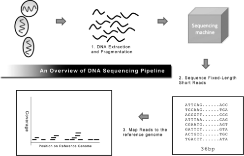
Figure 1: Overview of sequencing pipeline.

As noted in previous studies, sequencing coverage is dependent on characteristics of the local DNA sequence, and fluctuates even when there are no changes in copy number, as shown in Dohm et al. (2008). Just as adjusting for probe-effects is important for interpretation of microarray data, adjusting for these baseline fluctuations in depth of coverage is important for sequencing data. The bottom panels of Figure 3 show the varying depth of coverage for Chromosomes 8 and 11 in the sequencing of a normal human sample, HCC1954. Many factors cause the inhomogeneity of depth of coverage. For example, regions of the genome that contain more G/C bases are typically more difficult to fragment in an experiment. This results in lower depth of coverage in such regions. Some regions of the genome are highly repetitive. It is challenging to map reads from repetitive regions correctly onto the reference genome and, hence, some of the reads are inevitably discarded as unmappable, resulting in loss of coverage in that region, even though no actual deletion has occurred. Some ongoing efforts on the analysis of sequencing data involve modeling the effects of measurable quantities, such as GC content and mappability, on baseline depth. Cheung et al. (2011) demonstrated that read counts in sequencing are highly dependent on GC content and mappability, and discussed a method to account for such systematic biases. Benjamini and Speed (2011) investigated the relationship between GC content and read count on the Illumina sequencing platform with a single position model, and identified a family of unimodal curves that describes the effect of GC content on read count. We take the approach of empirically controlling for the baseline fluctuations by comparing the sample of interest to a control sample that was prepared and sequenced by the same protocol. In the context of tumor CNA detection, the control is preferably a matched normal sample, for it eliminates the discovery of germline copy number variants and allows one to focus on somatic CNA regions of the specific tumor genome. If a perfectly matched sample is not possible, a carefully chosen control or a pool of controls, with sequencing performed on the same platform with the same experimental protocol, would work for our method as well since almost all of the normal human genome are identical.

As a simple and illustrative example of the data, we generated points according to a nonhomogeneous Poisson Process. Figure 2 shows the point processes and the underlying $p(t)$ function, defined as the probability that a read at genomic position $t$ is from the case/tumor sample, conditional on the existence of a read at position $t$. The model is discussed in more detail in Section 3. The $y$-values for the points are jittered for graphical clarity.

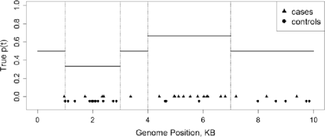
Figure 2: Illustration of paired Poisson Processes and $p(t)$.

Existing methods on CNV and CNA detection with sequencing data generally follow the change-point paradigm, which is natural since copy number changes reflect actual breakpoints along chromosomes. Chiang et al. (2009) proposed the algorithm SegSeq that segments the genomes of a tumor and a matched normal sample by using a sliding fixed size window, reducing the data to the ratio of read counts for each window. Xie and Tammi (2009) proposed CNV-seq that detects CNV regions between two individuals based on binning the read counts and then applying methods developed for array data. Yoon et al. (2009) designed a method named Event-Wise Testing (EWT) that detects CNV events using a fixed-window scan on the GC content adjusted read counts. Ivakhno et al. (2010) proposed a method called CNAseg that uses read counts in windows of predefined size, and discovers CNV using a Hidden Markov Model segmentation. As for single sample CNV detection method, Boeva et al. (2011) constructed a computational algorithm that normalizes read counts by GC content and estimates the absolute copy number.

These existing methods approach this statistical problem by binning or imposing fixed local windows. Some methods utilize the log ratio of read counts in the bin or window as a test statistic, thereby reducing the data to the familiar representation of array-based CNV/CNA detection, with Ivakhno et al. (2010) being an exception in that it uses the difference in tumor-normal window read counts in their HMM segmentation. There are a number of downsides to the binning or local window approach. First, due to the inhomogeneity of reads, certain bins will receive much larger number of reads overall than other bins, and the optimal window size varies across the genome. If the number of reads in a bin is not large enough, the normal approximations that are employed in many of these methods break down. Second, by binning or fixed-size window sliding, the estimated CNV/CNA boundaries can be imprecise if the actual breakpoints are not close to the bin or window boundary. This problem can be somewhat mitigated by refining the boundary after the change point is called, as done in SegSeq. In this paper, we propose a unified model, one that detects the change points, estimates their locations, and assesses their uncertainties simultaneously.

To illustrate and evaluate our method, we apply it to real and spiked-in data based on a pair of NCI-60 tumor/normal cell lines, HCC1954 and BL1954. The data for these samples were produced and investigated by Chiang et al. (2009). The whole-genome shotgun sequencing was performed on the Illumina platform and the reads are 36 bp long. After read and mapping quality exclusions, 7.72 million and 6.65 million reads were used for the tumor (HCC1954) and normal (BL1954) samples, respectively. Newer sequencing platforms produce much more massive data sets.

3 A change-point model on two nonhomogeneous Poisson processes

We start with a statistical model for the sequenced reads. Let $\{X_{t}|t\leq T\}$ and $\{Y_{t}|t\leq T\}$ be the number of reads whose first base maps to the left of base location $t$ of a given chromosome for the case and control samples, respectively. We can view these count processes as realizations of two nonhomogeneous Poisson processes (NHPP), one each for the case and control samples,

$$\{X_{t}\} \sim \operatorname{NHPP}(\mu_{t}),$$

$$\{Y_{t}\} \sim \operatorname{NHPP}(\lambda_{t}).$$

The scale $t$ is in base pairs. The scenario where two or more reads are mapped to the same genomic position is allowed by letting $\mu_{t}$ and $\lambda_{t}$ take values larger than 1 and assuming that the observed process is binned at the integers. We propose a change-point model on the conditional probability of an event at position $t$ being from $\{X_{t}\}$, given that there is such an event from either $\{X_{t}\}$ or $\{Y_{t}\}$, namely,

$$p(t)=\frac{\mu_{t}}{\mu_{t}+\lambda_{t}}=p_{k}\qquad\mbox{if }t_{k}\leq t<t_{k+1},k=1,\ldots,K.$$ (2)

An example of data according to this model is shown in Figure 2. The change-point model assumption can be equivalently expressed as

$$\mu_{t}=\lambda_{t}f(t),$$

where $f(t)=p(t)/[1-p(t)]$ is piecewise constant with change points $\{t_{k}\}$. Of course, we require the collection of change points to lie within the observation window:

$$0=t_{0}<t_{1}<\cdots<t_{K+1}=T.$$

This model does not force the overall intensity of case and control reads to be the same. The intensity function $\lambda_{t}$ reflects the inhomogeneity of the control reads. One interpretation of the model is that, apart from constant shifts, the fluctuation of coverage in the case sample is the same as that in the control sample. This is reasonable if the case and control samples are prepared and sequenced by the same laboratory protocol and mapped by the same procedure, as we discussed in Section 2. The model would not be valid if the intensity functions for samples have significant differences caused by nonmatching protocols or experimental biases.

Let $\{U_{1},\ldots,U_{m_{1}}\}$, $\{V_{1},\ldots,V_{m_{2}}\}$ be the event locations for processes $\{X_{t}\}$ and $\{Y_{t}\}$, respectively. That is, $U$ and $V$ are the mapped positions of the reads from the case and control samples. Let $m=m_{1}+m_{2}$ be the total number of reads from the case and control samples combined. We combine the read positions from the case and control processes and keep them ordered in the genome position, obtaining combined read positions $W_{1},\ldots,W_{m}$ and indicators of whether each event is a realization of the case process or the control process $Z_{1},\ldots,Z_{m}$:

$$Z_{i}=\cases{1,&\quad$\mbox{if }W_{i}\in\{U_{1},\ldots,U_{m_{1}}\},$\vspace*{2pt}\cr 0,&\quad$\mbox{if }W_{i}\in\{V_{1},\ldots,V_{m_{2}}\}.$}$$ (3)

For any read $i$ in the combined process, we will sometimes use the term “success” to mean that $Z_{i}=1$, that is, that the read is from the case process. Notice that the collection of change-point locations that can be inferred with the data is precisely $\{W_{1},\ldots,W_{m}\}$, since we do not have data points to make inference in favor of or against any change points in between observations. This means that estimating the copy number between two genome positions is equivalent to doing so for the closest pair of reads that span the two genome positions of interest. Namely, there is a one-to-one correspondence between the set of possible change points on $\{W_{1},\ldots,W_{m}\}$ and the set of change points $\{1=\tau_{0}<\tau_{1}<\cdots<\tau_{K+1}=m\}$ defined on the indices $\{1,\ldots,m\}$ through the following:

$$\{\tau_{k}=j\}\Longleftrightarrow\{t_{k}=W_{j}\}.$$

The above statement can be made formal through the equivariance principle. Consider the sample space $[0,T]$ of any change point, any monotonically increasing function $\phi:[0,T]\rightarrow[0,T]$, and its natural vector extension $\bar{\phi}(c_{1},\ldots,c_{n})=(\phi(c_{1}),\ldots,\phi(c_{n}))$.

Definition 1.

A change-point estimator $\hat{\tau}$ is monotone transform equivariant if for all monotonically increasing functions $\phi:[0,T]\rightarrow[0,T]$, we have $\hat{\tau}(\bar{\phi}(U),\bar{\phi}(V))=\bar{\phi}(\hat{\tau}(U,V)).$

The following theorem shows that any breakpoint estimator $\hat{\tau}(U,V)$ satisfying the equivariance condition can be decomposed into a simpler form.

Theorem 1

Let $\hat{\tau}(U,V)$, which takes values in $W$, be an estimator of the breakpoints. Then $\hat{\tau}$ is monotone transform equivariant if and only if $\hat{\tau}(U,V)=W_{\hat{K}}$, where $\hat{K}=f(Z)$ taking integer values $\{1,\ldots,m\}$ does not depend on $W$.

For ease of notation, we let $\bar{\phi}(W)=(\phi(W_{1}),\ldots,\phi(W_{m}))$ be the natural extension of $\phi$. Suppose $\hat{\tau}(U,V)=W_{\hat{K}}$, where $\hat{K}=f(Z)$. Note that $Z$ is invariant to all monotone transformations of the arrival times, hence so is $\hat{K}$. Therefore, $\phi(\hat{\tau}(U,V))=\phi(W_{\hat{K}})=(\bar{\phi}(W))_{\hat{K}}=\hat{\tau}(\bar{\phi}(U),\bar{\phi}(V))$.

In the other direction, since $\hat{\tau}\in W$ and $(U,V)$ contain the same information as $(W,Z)$, we must have $\hat{\tau}(U,V)=W_{\hat{K}(W,Z)}$. Suppose that $\hat{K}(W,Z)$ depend on $W$ in a nontrivial way but $\hat{\tau}$ satisfies the monotone transform equivariance condition. This means that there exist $W^{\prime}\neq W$ such that $\hat{K}(W,Z)\neq\hat{K}(W^{\prime},Z)$. But since $W$ and $W^{\prime}$ are both increasing finite sequences on $[0,T]$ with the same number of elements, we must have some $\phi(\cdot)$ that $\bar{\phi}(W)=W^{\prime}$. Note that $(W^{\prime},Z)$ induces $(U^{\prime},V^{\prime})=(\bar{\phi}(U),\bar{\phi}(V))$. However, $\hat{\tau}(\bar{\phi}(U),\bar{\phi}(V))=\hat{\tau}(U^{\prime},V^{\prime})=W^{\prime}_{\hat{K}(W^{\prime},Z)}=\phi(W_{\hat{K}(W^{\prime},Z)})\neq\phi(W_{\hat{K}(W,Z)})=\break\phi(\hat{\tau}(U,V))$. Hence, the equivariance property holds if and only if $\hat{K}$ is only a function of $Z$.

Theorem 1 implies that any breakpoint estimation procedure, that is, monotone transform equivariant uses the estimator $\hat{K}$ of integer breakpoints based on $Z$, and that the actual read position $W$ merely serves as a genomic scale lookup table. Hence, we can define our change-point model on the indices $\{1,\ldots,m\}$ for the read counts, and use the conditional likelihood which depends only on $\{Z_{i}\}$ but not on the event positions $\{W_{1},\ldots,W_{m}\}$:

$$p(j)=p_{k}\qquad\mbox{if }\tau_{k}\leq j<\tau_{k+1}.$$ (4)

For the rest of this section, we will exclusively work with equation (4). The mapping positions $\{W_{1},\ldots,W_{m}\}$ will re-enter our analysis when we compute confidence intervals for the copy number estimates, in Section 4. Our statistical problem is hence two-fold. First, given $K$, we need to estimate the change points $\{\tau_{k}\}$. Second, we need a method to select model complexity, as dictated by $K$.

We start by considering the following simplified problem: Given a single interval spanning reads $i$ to $j$ in the combined process, we want to test whether the success probability inside this interval, $p_{ij}$, is different from the overall success probability, $p$. The null model $H_{0}$ states that $p_{ij}=p$. We derive two statistics to test this hypothesis. The first is adopted from the conditional score statistic for a general exponential family model where the signal is represented by a kernel function, as discussed in Rabinowitz (1994),

$$\qquad S_{ij}=\sum_{k=1}^{m}(Z_{k}-\hat{p})\Biggl{(}1_{i\leq k\leq j}-\frac{1}{m}\sum_{k=1}^{m}1_{i\leq k\leq j}\Biggr{)}=\sum_{i\leq k\leq j}Z_{k}-\hat{p}(j-i+1),$$ (5)

where $\hat{p}=\sum{Z_{k}}/m$. This statistic is simply the difference between the number of observed and expected case events under the null model. Its variance at the null is

$$\hat{\sigma}_{ij}^{2}=\operatorname{Var}(S_{ij})=\biggl{(}1-\frac{j-i+1}{m}\biggr{)}(j-i+1)p(1-p)$$

and is used to standardize $S_{ij}$ for comparison between regions of different sizes. The standardized score statistic $T_{ij}=S_{ij}/\sigma_{ij}$ is intuitive and simple, and would be approximately standard normal if $j-i$ were large. However, the normal approximation is not accurate if the number of reads that map to the region is low. To attain higher accuracy for regions with low read count, observe that $\sum_{i\leq k\leq j}Z_{k}$ is a binomial random variable, and use an exact binomial generalized likelihood ratio (GLR) statistic,

$$\Lambda_{ij}=\sup_{p_{0},p_{ij}}l_{1}(p_{0},p_{ij})-\sup_{p}l_{0}(p),$$

where the null model with one overall success probability parameter $p$ is compared with the alternative model with one parameter $p_{ij}$ for inside the $[i,j]$ interval and another parameter $p_{0}$ for outside the interval. From the binomial log-likelihood function one obtains

$$\Lambda_{ij} = \sum_{k\in[i,j]}\biggl{\{}Z_{k}\log\biggl{(}\frac{\hat{p}_{ij}}{\hat{p}}\biggr{)}+(1-Z_{k})\log\biggl{(}\frac{1-\hat{p}_{ij}}{1-\hat{p}}\biggr{)}\biggr{\}}$$

$${}+\sum_{k\notin[i,j]}\biggl{\{}Z_{k}\log\biggl{(}\frac{\hat{p}_{0}}{\hat{p}}\biggr{)}+(1-Z_{k})\log\biggl{(}\frac{1-\hat{p}_{0}}{1-\hat{p}}\biggr{)}\biggr{\}},$$

where $\hat{p}$, $\hat{p}_{0}$, $\hat{p}_{ij}$ are maximum likelihood estimates of success probabilities

$$\hat{p} = \sum_{k=1}^{m}Z_{k}/m,$$

$$\hat{p}_{ij} = \sum_{k\in[i,j]}Z_{k}/(j-i+1),$$

$$\hat{p}_{0} = \sum_{k\notin[i,j]}Z_{k}/(m-j+i-1).$$

The GLR and score statistics allow us to measure how distinct a specific interval $[i,j]$ is compared to the entire chromosome. For the more general problem in which $(i,j)$ is not given but only one such pair exists, we compute the statistic for all unique pairs of $(i,j)$ to find the most significantly distinct interval. This operation is $O(m^{2})$ and to improve efficiency, we have implemented a search-refinement scheme called Iterative Grid Scan in our software. It works by identifying larger interesting intervals on a coarse grid and then iteratively improving the interval boundary estimates. The computational complexity is roughly $O(m\log m)$ and hence scales easily. A similar idea was studied in Walther (2010).

In the general model with multiple unknown change points, one could theoretically estimate all change points simultaneously by searching through all possible combinations of $\{\hat{\tau}_{k}\}$. But this is a combinatorial problem where even the best dynamic programming solution [Bellman (1961); Bai and Perron (2003); Lavielle (2005)] would not scale well for a data set containing millions of reads. Thus, we adapted Circular Binary Segmentation [Olshen et al. (2004); Venkatraman and Olshen (2007)] to our change-point model as a greedy alternative. In short, we find the most significant region $(i,j)$ over the entire chromosome, which divides the chromosome in to 3 regions (or two, if one of the change points lies on the edge). Then we further scan each of the regions, yielding a candidate subinterval in each region. At each step, we add the most significant change point(s) over all of the regions to the collection of change-point calls.

Model complexity grows as we introduce more change points. This brings us to the issue of model selection: We need a method to choose an appropriate number of change points $K$. Zhang and Siegmund (2007) proposed a solution to this problem for Gaussian change-point models with shifts in mean. Like the Gaussian model, the Poisson change-point model has irregularities that make classic measures such as the AIC and the BIC inappropriate. An extension of Zhang and Siegmund (2007) gives a Modified Bayes Information Criterion (mBIC) for our model, derived as a large sample approximation to the Bayes Factor in the spirit of Schwarz (1978):

$$\operatorname{mBIC}(K) = \log\biggl{(}\frac{\sup_{p(t),\tau}L(p(t),\tau)}{\sup_{p}L(p)}\biggr{)}-\frac{1}{2}\sum_{k=0}^{K}\log(\hat{\tau}_{k+1}-\hat{\tau}_{k})$$

$${}+\frac{1}{2}\log(m)-K\log(m^{\prime}),$$

where $m^{\prime}$ is the number of unique values in $\{W_{1},\ldots,W_{m}\}$.

The first term of mBIC is the generalized log-likelihood ratio for the model with $K$ change points versus the null model with no change points. In our context, $K$ ideally reflects the number of biological breakpoints that yield the copy number variants. The remaining terms can be interpreted as a “penalty” for model complexity. These penalty terms differ from the penalty term in the classic BIC of Schwarz (1978) due to nondifferentiability of the likelihood function in the change-point parameters $\{\tau_{k}\},$ and also due to the fact that the range of values for $\{\tau_{k}\}$ grow with the number of observations $m$. For more details on the interpretation of the terms in the mBIC, see Zhang and Siegmund (2007). Finally, we report the segmentation with $\widehat{{K}}={\arg\max}_{K}\operatorname{mBIC}(K)$ change points.

4 Approximate Bayesian confidence intervals

As noted in the Introduc-tion, it is particularly important for sequencing data to assess the uncertainty in the relative read intensity function at each genomic position. We approach this problem by constructing approximate Bayesian confidence intervals.

Suppose $Z_{1},\ldots,Z_{m}$ are independent realizations of Bernoulli random variables with success probabilities $\{p_{t}\}$. Consider first the one change-point model (which can be seen as a local part of a multiple change-point model), where

$$p_{t}=\cases{p_{0},&\quad$\mbox{if }t\leq\tau,$\vspace*{2pt}\cr p_{1},&\quad$\mbox{if }t>\tau.$}$$

Without loss of generality, we may take $\tau\in\{1,2,\ldots,m\}$. Assume a uniform prior for $\tau$ on this discrete set. Let $S_{t}$ be the number of successes up to and including the $t$th realization,

$$S_{t}=\sum_{1\leq i\leq t}Z_{i}.$$

Our goal is to construct confidence bands for $p_{t}$ at each $t\in\{1,2,\ldots,m\}$. Assume a $\operatorname{Beta}(\alpha,\beta)$ prior for $p_{0}$ and $p_{1}$. If we knew $\tau$, then the posterior distribution of $p_{0}$ and $p_{1}$ is

$$f(p_{0}|\vec{Z},\tau=\tau^{*}) \propto f(p_{0})f(S_{\tau^{*}}|p_{0})$$

$$\sim \operatorname{Beta}(\alpha,\beta)\cdot\operatorname{Binom}(S_{\tau^{*}};\tau^{*},p_{0})$$

$$\sim \operatorname{Beta}(\alpha+S_{\tau^{*}},\beta+\tau^{*}-S_{\tau^{*}}),$$

$$f(p_{1}|\vec{Z},\tau=\tau^{*}) \propto f(p_{1})f(S_{m}-S_{\tau^{*}}|p_{1})$$

$$\sim \operatorname{Beta}(\alpha+S_{m}-S_{\tau^{*}},\beta+m-\tau^{*}-S_{m}+S_{\tau^{*}}).$$

Now, without knowing the actual $\tau^{*}$, we compute the posterior distribution of $p_{t}$ as

$$f(p_{t}|\vec{Z}) = \sum_{i=1}^{m}f(p_{t},\tau=i|\vec{Z})$$

$$= \sum_{i=1}^{m}f(p_{t}|\tau=i,\vec{Z})\cdot f(\tau=i|\vec{Z}).$$

As before, the first part of the summation term is a beta distribution,

$$f(p_{t}|\tau=i,\vec{Z})=\cases{\operatorname{Beta}(\alpha+S_{i},\beta+i-S_{i}),&\quad$\mbox{if }t\leq i,$\vspace*{2pt}\cr\operatorname{Beta}(\alpha+S_{m}-S_{i},\beta+m-i-S_{m}+S_{i}),&\quad$\mbox{if }t>i,$}$$

and for the second term, we define the likelihood of the change point at $i$ as $L_{i}=f(\vec{Z}|\tau=i)$ and observe that with the uniform prior on $\tau$,

$$f(\tau=i|\vec{Z})\propto L_{i}/m\propto L_{i},$$

where

$$L_{i}=\int\prod_{1\leq j\leq i}p_{0}^{Z_{j}}(1-p_{0})^{1-Z_{j}}\,dP_{0}\cdot\int\prod_{i<j\leq m}p_{1}^{Z_{j}}(1-p_{1})^{1-Z_{j}}\,dP_{1},$$ (6)

and $dP_{0}$ and $dP_{1}$ are with respect to the prior distributions of $p_{0}$ and $p_{1}$. With $\operatorname{Beta}(\alpha,\beta)$ priors on $p_{0}$ and $p_{1}$, we can find the closed form expression of $L_{i}$:

$$L_{i} = \int\prod_{1\leq j\leq i}p_{0}^{Z_{j}}(1-p_{0})^{1-Z_{j}}\,dP_{0}\cdot\int\prod_{i<j\leq m}p_{1}^{Z_{j}}(1-p_{1})^{1-Z_{j}}\,dP_{1}$$

$$= \frac{1}{B(\alpha,\beta)}\int p_{0}^{S_{i}}(1-p_{0})^{i-S_{i}}p_{0}^{\alpha-1}(1-p_{0})^{\beta-1}\,dp_{0}$$

$${}\times\frac{1}{B(\alpha,\beta)}\int p_{1}^{S_{m}-S_{i}}(1-p_{1})^{m-i-S_{m}+S_{i}}p_{1}^{\alpha-1}(1-p_{1})^{\beta-1}\,dp_{1}$$

$$= \frac{B(\alpha+S_{i},\beta+i-S_{i})B(\alpha+S_{m}-S_{i},\beta+m-i-S_{m}+S_{i})}{B(\alpha,\beta)^{2}}$$

$$= \frac{\Gamma(\alpha+S_{i})\Gamma(\beta+i-S_{i})}{\Gamma(\alpha+\beta+i)}$$

$${}\times\frac{\Gamma(\alpha+S_{m}-S_{i})\Gamma(\beta+m-i-S_{m}+S_{i})}{\Gamma(\alpha+\beta+m-i)}\frac{\Gamma(\alpha+\beta)^{2}}{\Gamma(\alpha)^{2}\Gamma(\beta)^{2}}.$$

Hence, we can compute, without knowing the actual value of $\tau$,

$$f(p_{t}|\vec{Z})\propto\sum_{i=1}^{m}f(p_{t}|\tau=i,\vec{Z})\cdot\frac{L_{i}}{L_{\hat{\tau}}}\qquad\mbox{where }\hat{\tau}=\arg\max_{i}L_{i}.$$ (8)

Observe that the posterior distribution is a mixture of $\operatorname{Beta}(\cdot,\cdot)$ distributions. In theory, we could compute weights $w_{i}=L_{i}/L_{\hat{\tau}}$ for all positions $i$ and then numerically compute $(\frac{\alpha}{2},1-\frac{\alpha}{2})$ quantiles of the posterior beta mixture distribution to obtain the Bayesian confidence intervals. However, in practice, one can approximate the sum in (8) by

$$f(p_{t}|\vec{Z})\approx\frac{1}{\sum_{w_{i}>\varepsilon}w_{i}}\biggl{[}\sum_{w_{i}>\varepsilon}w_{i}f(p_{t}|\tau=i,\vec{Z})\biggr{]},$$

for some small $\varepsilon>0$, hence ignoring the highly unlikely locations for the change points. Empirically, we use $\varepsilon=10^{-4}$. It is easy to see that the sequence of log likelihood ratios for alternative change points, $\log{\frac{L_{i}}{L_{\tau}}}$, form random walks with negative drift as $i$ moves away from the true change point $\tau$ [Hinkley (1970)]. The negative drift depends on the true $p_{0}$, $p_{1}$ and is larger in absolute magnitude when the difference between $p_{0}$ and $p_{1}$ is larger. With $\tau$ unknown, since $P(|\hat{\tau}-\tau|\leq\delta)$ can be made arbitrarily close to 1 for $\delta=o(m)$, one can make the same random walk construction for $\log(L_{i}/L_{\hat{\tau}})$ bounded away by $\delta$ from $\hat{\tau}$, as done in Cobb (1978). This implies that, for any $\varepsilon>0$, one may find a constant $c_{\varepsilon,p_{0},p_{1}}$ such that for any $i$ at least $c_{\varepsilon,p_{0},p_{1}}$ steps away from $\hat{\tau}$, $w_{i}<\varepsilon$ with probability approaching 1. Hence, it is reasonable to use a small cutoff to produce a close approximation to the posterior distribution.

The extension of this construction to multiple change points is straightforward. It entails augmenting the mixture components of one change point with that of its neighboring change points. This gives a computationally efficient way of approximating the Bayesian confidence interval using, typically, a few hundred mixture components, which has been implemented in seqCBS. There is also an extensive body of literature on constructing confidence intervals and confidence sets for estimators of the change point $\tau$. We refer interested readers to Siegmund (1988b) for discussion and efficiency comparison of various confidence sets in change-point problems.

5 Results

We first applied the proposed method to a matched pair of tumor and normal NCI-60 cell lines, HCC1954 and BL1954. Chiang et al. (2009) conducted the sequencing of these samples using the Illumina platform. For comparison with array-based copy number profiles on the same samples, we obtained array data on HCC1954 and BL1954 from the NCI-60 database at http://www.sanger.ac.uk/genetics/CGP/NCI60/. We applied the CBS algorithm [Olshen et al. (2004), Venkatraman and Olshen (2007)] with modified BIC stopping algorithm [Zhang and Siegmund (2007)] to estimate relative copy numbers based on the array data.

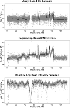
(a)	(b)

Figure 3: Comparison of seqCBS and array-based CN profiling. (a) HCC/BL1954 Chr 8, array, seqCBS, baseline read intensity. (b) HCC/BL1954 Chr 11, array, seqCBS, baseline read intensity.

Figure 3 shows the copy number profiles estimated from the array data (top) and from the sequencing data by seqCBS (middle), for two representative chromosomes where there appears to be a number of copy number alternation events. The bottom plots show the baseline $\lambda(t)$ function estimated by smoothing the binned counts of the normal sample sequencing data. There is clearly inhomogeneity in the rate function. The points for the top plots are normalized $\log$ ratios for the intensities of each probe on the array, whereas those for the middle plots are log ratios of binned counts for the tumor and normal samples. Note that the binned counts for the sequencing data are only for illustrative purposes, as the proposed method operates on the point processes directly, which are difficult to visualize at the whole-chromosome scale. The piecewise constant lines indicate the estimated $\log$ relative copy numbers and the change-point locations. Note that after adjusting for overall number of read differences between the two samples, the relative copy number is estimated by $\hat{p}(t)/(1-\hat{p}(t))$, where $\hat{p}(t)$ is the MLE estimate of the success probability of the segment into which $t$ falls.

The shape of the profile and overall locations for most change-point calls are common between the array and sequencing data. That is, CBS and SeqCBS applied on data generated from two distinct platforms generally agree. It is interesting that in the regions where a large number of CNA events seem to have occurred, our proposed method with sequencing is able to identify shorter and more pronounced CNA events. It also appears that the CNA calls based on sequencing are smoother in the sense that small magnitude shifts in array-based results, such as the change points after 102 Mb of Chromosome 11, are ignored by seqCBS. Similar observations can be made with results on other chromosomes as well. Since we do not know the ground truth in these tumor samples, it is hard to assess in more detail the performance of the estimates. Detailed spike-in simulation studies in the next section give a systematic view of the accuracy of the proposed method, as compared to the current standard approach.

Figure 4 is an example illustrating the approximate Bayesian confidence interval estimates around two CNA events on Chromosome 8 of HCC1954. This is not a typical example among the change-point calls. Typically, the signal differences are stronger and, hence, the confidence bands are narrower with little ambiguity region. The actual locations of mapped reads are shown as tick marks, with ticks at the bottom of the plot representing control reads, and ticks at the top representing case reads. The estimated relative copy numbers and their point-wise approximate Bayesian confidence intervals are shown as black and grey lines, respectively. One can see that the width of the confidence intervals depends not only on the number of reads in the segment, but also on the distance from the position of interest to the called change points, and that the confidence intervals are not necessarily symmetric around the estimated copy number.

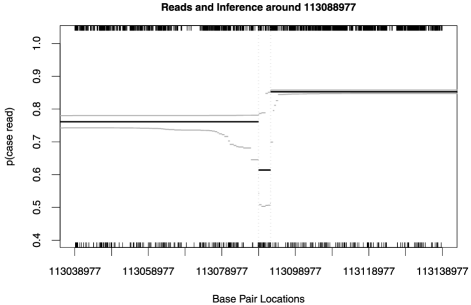
Figure 4: Bayesian CI, HCC1954 Chr 8. The solid black line is the estimated copy number, light gray lines are 95% confidence intervals. The actual locations of the case and control reads are shown as tick marks at the top and bottom of the plot, respectively.

6 Performance assessment

To assess the performance of the proposed method more precisely, we conducted a spike-in simulation study. We empirically estimated the underlying inhomogeneous rate function $\lambda(t)$ by kernel smoothing of the read counts from the normal sample, BL1954, in Chiang et al. (2009). The simulated tumor rate function $\mu(t)$ is then constructed by spiking into $\lambda(t)$ segments of single copy gain/loss. Since the length of the CNA events influences their ease of detection, we considered a range of different signal lengths. Each simulated case sample contains 50 changed segments. We compared seqCBS to SegSeq, which is one of the more popular available algorithms. For seqCBS, we used mBIC to determine appropriate model complexity. We used SegSeq with its default parameters. A change-point call was deemed true if it was within 100 reads of a true spike-in change point, after using a matching algorithm implemented in the R package clue by Hornik (2005, 2010) to find minimal-distance pairing between the called change points and the true change points. Performance was evaluated by recall and precision, defined respectively as the proportion of true signals called by the method and the proportion of signals called that are true. The simulation was repeated multiple times to reduce the variance in the performance measures.

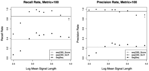
Figure 5: Recall and precision of seqCBS & SegSeq.

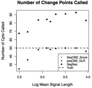
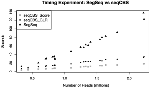
(a)	(b)

Figure 6: Model complexity and timing by seqCBS & SegSeq. (a) Model complexity comparison. (b) Timing comparison.

Figure 5 summarizes the performance comparison at default settings for a number of spike-in signal lengths. The horizontal lines are mean recall and precision rates for the methods. We see that SeqCBS, used with either the score test statistic or the GLR statistic, offers significant improvement over the existing method in both precision and recall. The performances of the score and GLR statistics are very similar, as their recall and precision curves almost overlap. The improvement in precision can be largely attributed to the fact that mBIC provides a good estimate of model complexity, as can be seen in Figure 6(a).

Table 1: Performance measures and tuning parameters. SegSeq: W${}={}$fixed local window size (default 500), A${}={}$number of false positive candidates for initialization (default 1000), B${}={}$number of false positive segments for termination (default 10). SeqCBS: Scr${}={}$score statistic, Bin${}={}$GLR statistic, G${}={}$IGS power step size (default 10); N/A values indicate program failures

Log mean breakpoint length
Length	$2.49$	$2.68$	$2.91$	$3.10$	$3.18$	$3.29$	$3.51$	$3.73$	$3.95$
Recall
SegSeq
Default	$0.066$	$0.146$	$0.394$	$0.514$	$0.464$	$0.476$	$0.502$	$0.438$	$0.424$
W250	$0.23$	$0.422$	$0.67$	$0.662$	$0.59$	$0.654$	$0.64$	$0.564$	$0.516$
W750	NA	NA	$0.148$	$0.206$	$0.248$	$0.36$	$0.408$	$0.384$	$0.346$
A500	NA	$0.148$	$0.394$	$0.514$	$0.464$	$0.476$	$0.502$	$0.438$	$0.424$
A2000	NA	$0.146$	$0.394$	$0.514$	$0.464$	$0.476$	$0.502$	$0.438$	$0.424$
B25	NA	$0.182$	$0.404$	$0.532$	$0.484$	$0.502$	$0.506$	$0.452$	$0.458$
B5	NA	$0.126$	$0.382$	$0.476$	$0.432$	$0.442$	$0.476$	$0.428$	$0.364$
SeqCBS
Scr-Def	$0.49$	$0.714$	$0.95$	$0.988$	$0.95$	$0.936$	$0.968$	$0.878$	$0.782$
Bin-Def	$0.492$	$0.718$	$0.948$	$0.99$	$0.956$	$0.936$	$0.968$	$0.876$	$0.81$
Scr-G5	$0.496$	$0.71$	$0.922$	$0.99$	$0.956$	$0.956$	$0.978$	$0.922$	$0.844$
Bin-G5	$0.496$	$0.712$	$0.928$	$0.99$	$0.958$	$0.962$	$0.98$	$0.946$	$0.844$
Scr-G15	$0.494$	$0.708$	$0.926$	$0.974$	$0.942$	$0.938$	$0.968$	$0.89$	$0.736$
Bin-G15	$0.496$	$0.716$	$0.93$	$0.976$	$0.946$	$0.96$	$0.972$	$0.91$	$0.748$
Precision
SegSeq
Default	$0.049$	$0.105$	$0.235$	$0.305$	$0.284$	$0.263$	$0.276$	$0.237$	$0.255$
W250	$0.174$	$0.317$	$0.490$	$0.472$	$0.467$	$0.478$	$0.442$	$0.405$	$0.399$
W750	NA	NA	$0.107$	$0.137$	$0.165$	$0.227$	$0.242$	$0.232$	$0.212$
A500	NA	$0.097$	$0.235$	$0.305$	$0.284$	$0.263$	$0.276$	$0.237$	$0.255$
A2000	NA	$0.101$	$0.235$	$0.305$	$0.284$	$0.263$	$0.276$	$0.237$	$0.255$
B25	NA	$0.101$	$0.203$	$0.278$	$0.254$	$0.243$	$0.246$	$0.219$	$0.240$
B5	NA	$0.104$	$0.278$	$0.361$	$0.323$	$0.308$	$0.327$	$0.295$	$0.271$
SeqCBS
Scr-Def	$0.980$	$0.997$	$0.985$	$0.988$	$0.985$	$0.944$	$0.968$	$0.878$	$0.839$
Bin-Def	$0.984$	$0.997$	$0.988$	$0.990$	$0.992$	$0.947$	$0.968$	$0.876$	$0.884$
Scr-G5	$0.984$	$0.997$	$0.956$	$0.990$	$0.992$	$0.980$	$0.994$	$0.945$	$0.942$
Bin-G5	$0.984$	$0.994$	$0.959$	$0.990$	$0.994$	$0.990$	$0.996$	$0.977$	$0.942$
Scr-G15	$0.980$	$0.994$	$0.953$	$0.944$	$0.961$	$0.949$	$0.964$	$0.876$	$0.710$
Bin-G15	$0.984$	$0.994$	$0.953$	$0.946$	$0.973$	$0.984$	$0.972$	$0.910$	$0.733$

We studied the performance sensitivity on tuning parameters. SegSeq allows three tuning parameters: local window size (W), number of false positive candidates for initialization (A), and number of false positive segments for termination (B). The proposed method has a step size parameter (G) that controls the trade-off between speed and accuracy in our Iterative Grid Scan component, and hence influences performance. We varied these parameters and recorded the performance measures in Table 1. It appears that local window size (W) is an important tuning parameter for SegSeq, and in scenarios with relatively short signal length, a smaller W${}={}$250 provides significant improvement in its performance. This echoes with our previous discussion that methods using a single fixed window size would perform less well when the signals are not of the corresponding length. Some of the parameter combinations for SegSeq result in program running errors in some scenarios, and are marked as NA. The step size parameter (G) in SeqCBS, in constrast, controls the rate at which coarse segment candidates are refined and the rate at which the program descends into searching smaller local change points, rather than defining a fixed window size. A smaller step size typically yields slightly better performance. However, the proposed method is not nearly as sensitive to its tuning parameters. We also conducted a timing experiment to provide the reader with a sense of the required computational resources to derive the solution. Our proposed method compares favorably with SegSeq as seen in Figure 6(b). The GLR statistic is slightly more complex to compute than the score statistic, as is reflected in the timing experiment. However, copy number profiling is inherently a highly parallelizable computing problem: one may distribute the task for each chromosome among a multi-CPU computing grid, hence dramatically reducing the amount of time required for this analysis.

7 Discussion

We proposed an approach based on nonhomogeneous Poisson Processes to directly model next-generation DNA sequencing data, and formulated a change-point model to conduct copy number profiling. The model yields simple score and generalized likelihood ratio statistics, as well as a modified Bayes information criterion for model selection. The proposed method has been applied to real sequencing data and its performance compares favorably to an existing method in a spike-in simulation study.

Statistical inference, in the form of confidence estimates, is very important for sequencing-based data, since, unlike arrays, the effective sample size (i.e., coverage) for estimating copy number varies substantially across the genome. In this paper, we derived a procedure to compute Bayesian confidence intervals on the estimated copy number. Other types of inference, such as $p$-values or confidence intervals on the estimated change points, may also be useful. Siegmund (1988b) compares different types of confidence intervals on the change points, and the methods there can be directly applied to this problem. The reader is referred to Rabinowitz (1994) and Siegmund (1988a) for existing methods on significance evaluation.

Some sequencing experiments produce paired end reads, where two short reads are performed on the two ends of a longer fragment of DNA. The pairing information can be quite useful in the profiling of structural genomic changes. It will be important to extend the approach in this paper to handle this more complex data type.

A limitation of the proposed method and the existing methods is that they do not handle allele-specific copy number variants. It is possible to extend our model to accommodate this need. With deep sequencing, one may assess whether each loci in a CNV is heterozygous, and estimate the degree to which each allele contributes to the gain or loss of copy number, by considering the number of reads covering the locus with the major allele versus those with the minor allele. This is particularly helpful for detecting deletion. Furthermore, in the context of assessing the allele-specific copy number, existing SNP arrays have the advantage that the assay targets specific sites for that problem, whereas to obtain sufficient evidence of allele-specific copy number variants with sequencing, a much greater coverage would be required since the overwhelming majority of reads would land in nonallelic genomic regions. Spatial models that borrow information across adjacent variant sites, such as Chen, Xing and Zhang (2011) and Olshen et al. (2011), would be helpful for improving power.

Recently, there has been increased attention to the problem of simultaneous segmentation of multiple samples [Lipson et al. (2006); Shah et al. (2007); Zhang et al. (2010); Siegmund, Yakir and Zhang (2011)]. One may also wish to extend this method to the multi-sample setting, where in addition to modeling challenges, one also needs to address more sources of systematic biases, such as batch effects and carry-over problems.

Computational challenges remain in this field. With sequencing capacity growing at record speed, even basic operations on the data set are resource-consuming. It is pertinent to develop faster and more parallelizable solutions to the copy number profiling problem.

References

- Bai and Perron (2003) {barticle}[author] \bauthor\bsnmBai, \bfnmJushan\binitsJ. and \bauthor\bsnmPerron, \bfnmP.\binitsP. (\byear2003). \btitleComputation and analysis of multiple structural change models. \bjournalJ. Appl. Econometrics \bvolume18 \bpages1–22. \bptokimsref \endbibitem
- Bellman (1961) {barticle}[author] \bauthor\bsnmBellman, \bfnmR.\binitsR. (\byear1961). \btitleOn the approximation of curves by line segments using dynamic programming. \bjournalCommun. ACM \bvolume4 \bpages284. \bptokimsref \endbibitem
- Benjamini and Speed (2011) {bmisc}[author] \bauthor\bsnmBenjamini, \bfnmY.\binitsY. and \bauthor\bsnmSpeed, \bfnmT.\binitsT. (\byear2011). \bhowpublishedEstimation and correction for GC-content bias in high throughput sequencing. Technical Report 804, Dept. Statistics, Univ. California, Berkeley. \bptokimsref \endbibitem
- Boeva et al. (2011) {barticle}[pbm] \bauthor\bsnmBoeva, \bfnmValentina\binitsV., \bauthor\bsnmZinovyev, \bfnmAndrei\binitsA., \bauthor\bsnmBleakley, \bfnmKevin\binitsK., \bauthor\bsnmVert, \bfnmJean-Philippe\binitsJ.-P., \bauthor\bsnmJanoueix-Lerosey, \bfnmIsabelle\binitsI., \bauthor\bsnmDelattre, \bfnmOlivier\binitsO. and \bauthor\bsnmBarillot, \bfnmEmmanuel\binitsE. (\byear2011). \btitleControl-free calling of copy number alterations in deep-sequencing data using GC-content normalization. \bjournalBioinformatics \bvolume27 \bpages268–269. \biddoi=10.1093/bioinformatics/btq635, issn=1367-4811, pii=btq635, pmcid=3018818, pmid=21081509 \bptokimsref \endbibitem
- Campbell et al. (2008) {barticle}[author] \bauthor\bsnmCampbell, \bfnmPeter J.\binitsP. J., \bauthor\bsnmStephens, \bfnmPhilip J.\binitsP. J., \bauthor\bsnmPleasance, \bfnmErin D.\binitsE. D., \bauthor\bsnmO’Meara, \bfnmSarah\binitsS., \bauthor\bsnmLi, \bfnmHeng\binitsH., \bauthor\bsnmSantarius, \bfnmThomas\binitsT., \bauthor\bsnmStebbings, \bfnmLucy A.\binitsL. A., \bauthor\bsnmLeroy, \bfnmCatherine\binitsC., \bauthor\bsnmEdkins, \bfnmSarah\binitsS., \bauthor\bsnmHardy, \bfnmClaire\binitsC., \bauthor\bsnmTeague, \bfnmJon W.\binitsJ. W., \bauthor\bsnmMenzies, \bfnmAndrew\binitsA., \bauthor\bsnmGoodhead, \bfnmIan\binitsI., \bauthor\bsnmTurner, \bfnmDaniel J.\binitsD. J., \bauthor\bsnmClee, \bfnmChristopher M.\binitsC. M., \bauthor\bsnmQuail, \bfnmMichael A.\binitsM. A., \bauthor\bsnmCox, \bfnmAntony\binitsA., \bauthor\bsnmBrown, \bfnmClive\binitsC., \bauthor\bsnmDurbin, \bfnmRichard\binitsR., \bauthor\bsnmHurles, \bfnmMatthew E.\binitsM. E., \bauthor\bsnmEdwards, \bfnmPaul A. W.\binitsP. A. W., \bauthor\bsnmBignell, \bfnmGraham R.\binitsG. R., \bauthor\bsnmStratton, \bfnmMichael R.\binitsM. R. and \bauthor\bsnmFutreal, \bfnmP. Andrew\binitsP. A. (\byear2008). \btitleIdentification of somatically acquired rearrangements in cancer using genome-wide massively parallel paired-end sequencing. \bjournalNature Genetics \bvolume40 \bpages722–729. \bptokimsref \endbibitem
- Chen, Xing and Zhang (2011) {barticle}[mr] \bauthor\bsnmChen, \bfnmHao\binitsH., \bauthor\bsnmXing, \bfnmHaipeng\binitsH. and \bauthor\bsnmZhang, \bfnmNancy R.\binitsN. R. (\byear2011). \btitleEstimation of parent specific DNA copy number in tumors using high-density genotyping arrays. \bjournalPLoS Comput. Biol. \bvolume7 \bpagese1001060, 15. \biddoi=10.1371/journal.pcbi.1001060, issn=1553-734X, mr=2776334 \bptokimsref \endbibitem
- Cheung et al. (2011) {barticle}[pbm] \bauthor\bsnmCheung, \bfnmMing-Sin\binitsM.-S., \bauthor\bsnmDown, \bfnmThomas A.\binitsT. A., \bauthor\bsnmLatorre, \bfnmIsabel\binitsI. and \bauthor\bsnmAhringer, \bfnmJulie\binitsJ. (\byear2011). \btitleSystematic bias in high-throughput sequencing data and its correction by BEADS. \bjournalNucleic Acids Res. \bvolume39 \bpagese103. \biddoi=10.1093/nar/gkr425, issn=1362-4962, pii=gkr425, pmcid=3159482, pmid=21646344 \bptokimsref \endbibitem
- Chiang et al. (2009) {barticle}[author] \bauthor\bsnmChiang, \bfnmDerek Y.\binitsD. Y., \bauthor\bsnmGetz, \bfnmGad\binitsG., \bauthor\bsnmJaffe, \bfnmDavid B.\binitsD. B., \bauthor\bsnmO’Kelly, \bfnmMichael J.\binitsM. J., \bauthor\bsnmZhao, \bfnmXiaojun\binitsX., \bauthor\bsnmCarter, \bfnmScott L.\binitsS. L., \bauthor\bsnmRuss, \bfnmCarsten\binitsC., \bauthor\bsnmNusbaum, \bfnmChad\binitsC., \bauthor\bsnmMeyerson, \bfnmMatthew\binitsM. and \bauthor\bsnmLander, \bfnmEric S.\binitsE. S. (\byear2009). \btitleHigh-resolution mapping of copy-number alterations with massively parallel sequencing. \bjournalNature Methods \bvolume6 \bpages99–103. \bptokimsref \endbibitem
- Cobb (1978) {barticle}[mr] \bauthor\bsnmCobb, \bfnmGeorge W.\binitsG. W. (\byear1978). \btitleThe problem of the Nile: Conditional solution to a changepoint problem. \bjournalBiometrika \bvolume65 \bpages243–251. \biddoi=10.1093/biomet/65.2.243, issn=0006-3444, mr=0513930 \bptokimsref \endbibitem
- Conrad et al. (2006) {barticle}[pbm] \bauthor\bsnmConrad, \bfnmDonald F.\binitsD. F., \bauthor\bsnmAndrews, \bfnmT. Daniel\binitsT. D., \bauthor\bsnmCarter, \bfnmNigel P.\binitsN. P., \bauthor\bsnmHurles, \bfnmMatthew E.\binitsM. E. and \bauthor\bsnmPritchard, \bfnmJonathan K.\binitsJ. K. (\byear2006). \btitleA high-resolution survey of deletion polymorphism in the human genome. \bjournalNat. Genet. \bvolume38 \bpages75–81. \biddoi=10.1038/ng1697, issn=1061-4036, pii=ng1697, pmid=16327808 \bptokimsref \endbibitem
- Dohm et al. (2008) {barticle}[pbm] \bauthor\bsnmDohm, \bfnmJuliane C.\binitsJ. C., \bauthor\bsnmLottaz, \bfnmClaudio\binitsC., \bauthor\bsnmBorodina, \bfnmTatiana\binitsT. and \bauthor\bsnmHimmelbauer, \bfnmHeinz\binitsH. (\byear2008). \btitleSubstantial biases in ultra-short read data sets from high-throughput DNA sequencing. \bjournalNucleic Acids Res. \bvolume36 \bpagese105. \biddoi=10.1093/nar/gkn425, issn=1362-4962, pii=gkn425, pmcid=2532726, pmid=18660515 \bptokimsref \endbibitem
- Hinkley (1970) {barticle}[mr] \bauthor\bsnmHinkley, \bfnmDavid V.\binitsD. V. (\byear1970). \btitleInference about the change-point in a sequence of random variables. \bjournalBiometrika \bvolume57 \bpages1–17. \bidissn=0006-3444, mr=0273727 \bptokimsref \endbibitem
- Hornik (2005) {barticle}[author] \bauthor\bsnmHornik, \bfnmKurt\binitsK. (\byear2005). \btitleA CLUE for CLUster Ensembles. \bjournalJournal of Statistical Software \bvolume14. \bptokimsref \endbibitem
- Hornik (2010) {bmisc}[author] \bauthor\bsnmHornik, \bfnmKurt\binitsK. (\byear2010). \bhowpublishedclue: Cluster ensembles R package version 0.3-34. \bptokimsref \endbibitem
- Ivakhno et al. (2010) {barticle}[pbm] \bauthor\bsnmIvakhno, \bfnmSergii\binitsS., \bauthor\bsnmRoyce, \bfnmTom\binitsT., \bauthor\bsnmCox, \bfnmAnthony J.\binitsA. J., \bauthor\bsnmEvers, \bfnmDirk J.\binitsD. J., \bauthor\bsnmCheetham, \bfnmR. Keira\binitsR. K. and \bauthor\bsnmTavaré, \bfnmSimon\binitsS. (\byear2010). \btitleCNAseg–a novel framework for identification of copy number changes in cancer from second-generation sequencing data. \bjournalBioinformatics \bvolume26 \bpages3051–3058. \biddoi=10.1093/bioinformatics/btq587, issn=1367-4811, pii=btq587, pmid=20966003 \bptokimsref \endbibitem
- Khaja et al. (2007) {barticle}[author] \bauthor\bsnmKhaja, \bfnmR.\binitsR., \bauthor\bsnmZhang, \bfnmJ.\binitsJ., \bauthor\bsnmMacDonald, \bfnmJ. R.\binitsJ. R., \bauthor\bsnmHe, \bfnmY.\binitsY., \bauthor\bsnmJoseph-George, \bfnmA. M.\binitsA. M., \bauthor\bsnmWei, \bfnmJ.\binitsJ., \bauthor\bsnmRafiq, \bfnmQian C.\binitsQ. C. \bsuffixM. A., \bauthor\bsnmShago, \bfnmM.\binitsM., \bauthor\bsnmPantano, \bfnmL.\binitsL., \bauthor\bsnmAburatani, \bfnmH.\binitsH., \bauthor\bsnmJones, \bfnmK.\binitsK., \bauthor\bsnmRedon, \bfnmR.\binitsR., \bauthor\bsnmHurles, \bfnmM.\binitsM., \bauthor\bsnmArmengol, \bfnmL.\binitsL., \bauthor\bsnmEstivill, \bfnmX.\binitsX., \bauthor\bsnmMural, \bfnmR. J.\binitsR. J., \bauthor\bsnmLee, \bfnmC\binitsC., \bauthor\bsnmScherer, \bfnmSW\binitsS. and \bauthor\bsnmFeuk, \bfnmL.\binitsL. (\byear2007). \btitleGenome assembly comparison to identify structural variants in the human genome. \bjournalNature Genetics \bvolume38 \bpages1413–1418. \bptokimsref \endbibitem
- Lai, Xing and Zhang (2007) {barticle}[author] \bauthor\bsnmLai, \bfnmT. L.\binitsT. L., \bauthor\bsnmXing, \bfnmH.\binitsH. and \bauthor\bsnmZhang, \bfnmN. R.\binitsN. R. (\byear2007). \btitleStochastic segmentation models for array-based comparative genomic hybridization data analysis. \bjournalBiostatistics \bvolume9 \bpages290–307. \bptokimsref \endbibitem
- Lai et al. (2005) {barticle}[pbm] \bauthor\bsnmLai, \bfnmWeil R.\binitsW. R., \bauthor\bsnmJohnson, \bfnmMark D.\binitsM. D., \bauthor\bsnmKucherlapati, \bfnmRaju\binitsR. and \bauthor\bsnmPark, \bfnmPeter J.\binitsP. J. (\byear2005). \btitleComparative analysis of algorithms for identifying amplifications and deletions in array CGH data. \bjournalBioinformatics \bvolume21 \bpages3763–3770. \biddoi=10.1093/bioinformatics/bti611, issn=1367-4803, mid=NIHMS171393, pii=bti611, pmcid=2819184, pmid=16081473 \bptokimsref \endbibitem
- Lavielle (2005) {barticle}[author] \bauthor\bsnmLavielle, \bfnmM.\binitsM. (\byear2005). \btitleUsing penalized contrasts for the change-point problem. \bjournalSignal Processing \bvolume85 \bpages1501–1510. \bptokimsref \endbibitem
- Lipson et al. (2006) {barticle}[mr] \bauthor\bsnmLipson, \bfnmDoron\binitsD., \bauthor\bsnmAumann, \bfnmYonatan\binitsY., \bauthor\bsnmBen-Dor, \bfnmAmir\binitsA., \bauthor\bsnmLinial, \bfnmNathan\binitsN. and \bauthor\bsnmYakhini, \bfnmZohar\binitsZ. (\byear2006). \btitleEfficient calculation of interval scores for DNA copy number data analysis. \bjournalJ. Comput. Biol. \bvolume13 \bpages215–228 (electronic). \bidissn=1066-5277, mr=2255255 \bptokimsref \endbibitem
- McCarroll et al. (2006) {barticle}[author] \bauthor\bsnmMcCarroll, \bfnmS. A.\binitsS. A., \bauthor\bsnmHadnott, \bfnmT. N.\binitsT. N., \bauthor\bsnmPerry, \bfnmG. H.\binitsG. H., \bauthor\bsnmSabeti, \bfnmP. C.\binitsP. C., \bauthor\bsnmZody, \bfnmM. C.\binitsM. C., \bauthor\bsnmBarrett, \bfnmJ. C.\binitsJ. C., \bauthor\bsnmDallaire, \bfnmS.\binitsS., \bauthor\bsnmGabriel, \bfnmS. B.\binitsS. B., \bauthor\bsnmLee, \bfnmC.\binitsC., \bauthor\bsnmDaly, \bfnmM. J.\binitsM. J., \bauthor\bsnmAltshuler, \bfnmD. M.\binitsD. M. and \bauthor\bsnmThe International HapMap Consortium (\byear2006). \btitleCommon deletion polymorphisms in the human genome. \bjournalNature Genetics \bvolume38 \bpages86–92. \bptokimsref \endbibitem
- Medvedev, Stanciu and Brudno (2009) {barticle}[pbm] \bauthor\bsnmMedvedev, \bfnmPaul\binitsP., \bauthor\bsnmStanciu, \bfnmMonica\binitsM. and \bauthor\bsnmBrudno, \bfnmMichael\binitsM. (\byear2009). \btitleComputational methods for discovering structural variation with next-generation sequencing. \bjournalNat. Methods \bvolume6 \bpagesS13–S20. \biddoi=10.1038/nmeth.1374, issn=1548-7105, pii=nmeth.1374, pmid=19844226 \bptokimsref \endbibitem
- Olshen et al. (2004) {barticle}[pbm] \bauthor\bsnmOlshen, \bfnmAdam B.\binitsA. B., \bauthor\bsnmVenkatraman, \bfnmE. S.\binitsE. S., \bauthor\bsnmLucito, \bfnmRobert\binitsR. and \bauthor\bsnmWigler, \bfnmMichael\binitsM. (\byear2004). \btitleCircular binary segmentation for the analysis of array-based DNA copy number data. \bjournalBiostatistics \bvolume5 \bpages557–572. \biddoi=10.1093/biostatistics/kxh008, issn=1465-4644, pii=5/4/557, pmid=15475419 \bptokimsref \endbibitem
- Olshen et al. (2011) {barticle}[pbm] \bauthor\bsnmOlshen, \bfnmAdam B.\binitsA. B., \bauthor\bsnmBengtsson, \bfnmHenrik\binitsH., \bauthor\bsnmNeuvial, \bfnmPierre\binitsP., \bauthor\bsnmSpellman, \bfnmPaul T.\binitsP. T., \bauthor\bsnmOlshen, \bfnmRichard A.\binitsR. A. and \bauthor\bsnmSeshan, \bfnmVenkatraman E.\binitsV. E. (\byear2011). \btitleParent-specific copy number in paired tumor-normal studies using circular binary segmentation. \bjournalBioinformatics \bvolume27 \bpages2038–2046. \biddoi=10.1093/bioinformatics/btr329, issn=1367-4811, pii=btr329, pmcid=3137217, pmid=21666266 \bptokimsref \endbibitem
- Rabinowitz (1994) {bincollection}[mr] \bauthor\bsnmRabinowitz, \bfnmDaniel\binitsD. (\byear1994). \btitleDetecting clusters in disease incidence. In \bbooktitleChange-Point Problems (South Hadley, MA, 1992). \bseriesInstitute of Mathematical Statistics Lecture Notes—Monograph Series \bvolume23 \bpages255–275. \bpublisherIMS, \baddressHayward, CA. \biddoi=10.1214/lnms/1215463129, mr=1477929 \bptokimsref \endbibitem
- Redon et al. (2006) {barticle}[author] \bauthor\bsnmRedon, \bfnmRichard\binitsR., \bauthor\bsnmIshikawa, \bfnmShumpei\binitsS., \bauthor\bsnmFitch, \bfnmKaren R.\binitsK. R., \bauthor\bsnmFeuk, \bfnmLars\binitsL., \bauthor\bsnmPerry, \bfnmGeorge H.\binitsG. H., \bauthor\bsnmAndrews, \bfnmDaniel T.\binitsD. T., \bauthor\bsnmFiegler, \bfnmHeike\binitsH., \bauthor\bsnmShapero, \bfnmMichael H.\binitsM. H., \bauthor\bsnmCarson, \bfnmAndrew R.\binitsA. R., \bauthor\bsnmChen, \bfnmWenwei\binitsW., \bauthor\bsnmCho, \bfnmEun K.\binitsE. K., \bauthor\bsnmDallaire, \bfnmStephanie\binitsS., \bauthor\bsnmFreeman, \bfnmJennifer L.\binitsJ. L., \bauthor\bsnmGonzalez, \bfnmJuan R.\binitsJ. R., \bauthor\bsnmGratacos, \bfnmMonica\binitsM., \bauthor\bsnmHuang, \bfnmJing\binitsJ., \bauthor\bsnmKalaitzopoulos, \bfnmDimitrios\binitsD., \bauthor\bsnmKomura, \bfnmDaisuke\binitsD., \bauthor\bsnmMacdonald, \bfnmJeffrey R.\binitsJ. R., \bauthor\bsnmMarshall, \bfnmChristian R.\binitsC. R., \bauthor\bsnmMei, \bfnmRui\binitsR., \bauthor\bsnmMontgomery, \bfnmLyndal\binitsL., \bauthor\bsnmNishimura, \bfnmKunihiro\binitsK., \bauthor\bsnmOkamura, \bfnmKohji\binitsK., \bauthor\bsnmShen, \bfnmFan\binitsF., \bauthor\bsnmSomerville, \bfnmMartin J.\binitsM. J., \bauthor\bsnmTchinda, \bfnmJoelle\binitsJ., \bauthor\bsnmValsesia, \bfnmArmand\binitsA., \bauthor\bsnmWoodwark, \bfnmCara\binitsC., \bauthor\bsnmYang, \bfnmFengtang\binitsF., \bauthor\bsnmZhang, \bfnmJunjun\binitsJ., \bauthor\bsnmZerjal, \bfnmTatiana\binitsT., \bauthor\bsnmZhang, \bfnmJane\binitsJ., \bauthor\bsnmArmengol, \bfnmLluis\binitsL., \bauthor\bsnmConrad, \bfnmDonald F.\binitsD. F., \bauthor\bsnmEstivill, \bfnmXavier\binitsX., \bauthor\bsnmTyler-Smith, \bfnmChris\binitsC., \bauthor\bsnmCarter, \bfnmNigel P.\binitsN. P., \bauthor\bsnmAburatani, \bfnmHiroyuki\binitsH., \bauthor\bsnmLee, \bfnmCharles\binitsC., \bauthor\bsnmJones, \bfnmKeith W.\binitsK. W., \bauthor\bsnmScherer, \bfnmStephen W.\binitsS. W. and \bauthor\bsnmHurles, \bfnmMatthew E.\binitsM. E. (\byear2006). \btitleGlobal variation in copy number in the human genome. \bjournalNature \bvolume444 \bpages444–454. \bptokimsref \endbibitem
- Schwarz (1978) {barticle}[mr] \bauthor\bsnmSchwarz, \bfnmGideon\binitsG. (\byear1978). \btitleEstimating the dimension of a model. \bjournalAnn. Statist. \bvolume6 \bpages461–464. \bidissn=0090-5364, mr=0468014 \bptokimsref \endbibitem
- Shah et al. (2007) {barticle}[author] \bauthor\bsnmShah, \bfnmS. P.\binitsS. P., \bauthor\bsnmLam, \bfnmW. L.\binitsW. L., \bauthor\bsnmNg, \bfnmR. T.\binitsR. T. and \bauthor\bsnmMurphy, \bfnmK. P.\binitsK. P. (\byear2007). \btitleModeling recurrent DNA copy number alterations in array CGH data. \bjournalBioinformatics \bvolume23 \bpages450–458. \bptokimsref \endbibitem
- Siegmund (1988a) {barticle}[mr] \bauthor\bsnmSiegmund, \bfnmDavid\binitsD. (\byear1988a). \btitleApproximate tail probabilities for the maxima of some random fields. \bjournalAnn. Probab. \bvolume16 \bpages487–501. \bidissn=0091-1798, mr=0929059 \bptokimsref \endbibitem
- Siegmund (1988b) {barticle}[mr] \bauthor\bsnmSiegmund, \bfnmDavid\binitsD. (\byear1988b). \btitleConfidence sets in change-point problems. \bjournalInternat. Statist. Rev. \bvolume56 \bpages31–48. \biddoi=10.2307/1403360, issn=0306-7734, mr=0963139 \bptokimsref \endbibitem
- Siegmund, Yakir and Zhang (2011) {barticle}[author] \bauthor\bsnmSiegmund, \bfnmD. O.\binitsD. O., \bauthor\bsnmYakir, \bfnmB.\binitsB. and \bauthor\bsnmZhang, \bfnmN. R.\binitsN. R. (\byear2011). \btitleDetecting simultaneous variant intervals in aligned sequences. \bjournalAnn. Appl. Stat. \bvolume5 \bpages645–668. \bidmr=2840169 \bptokimsref \endbibitem
- Venkatraman and Olshen (2007) {barticle}[pbm] \bauthor\bsnmVenkatraman, \bfnmE. S.\binitsE. S. and \bauthor\bsnmOlshen, \bfnmAdam B.\binitsA. B. (\byear2007). \btitleA faster circular binary segmentation algorithm for the analysis of array CGH data. \bjournalBioinformatics \bvolume23 \bpages657–663. \biddoi=10.1093/bioinformatics/btl646, issn=1367-4811, pii=btl646, pmid=17234643 \bptokimsref \endbibitem
- Walther (2010) {barticle}[mr] \bauthor\bsnmWalther, \bfnmGuenther\binitsG. (\byear2010). \btitleOptimal and fast detection of spatial clusters with scan statistics. \bjournalAnn. Statist. \bvolume38 \bpages1010–1033. \biddoi=10.1214/09-AOS732, issn=0090-5364, mr=2604703 \bptokimsref \endbibitem
- Wang et al. (2005) {barticle}[author] \bauthor\bsnmWang, \bfnmP.\binitsP., \bauthor\bsnmKim, \bfnmY.\binitsY., \bauthor\bsnmPollack, \bfnmJ.\binitsJ., \bauthor\bsnmNarasimhan, \bfnmB.\binitsB. and \bauthor\bsnmTibshirani, \bfnmR.\binitsR. (\byear2005). \btitleA method for calling gains and losses in array-CGH data. \bjournalBiostatistics \bvolume6 \bpages45–58. \bptokimsref \endbibitem
- Willenbrock and Fridlyand (2005) {barticle}[author] \bauthor\bsnmWillenbrock, \bfnmH.\binitsH. and \bauthor\bsnmFridlyand, \bfnmJ.\binitsJ. (\byear2005). \btitleA comparison study: Applying segmentation to arrayCGH data for downstream analyses. \bjournalBioinformatics \bvolume21 \bpages4084–4091. \bptokimsref \endbibitem
- Xie and Tammi (2009) {barticle}[pbm] \bauthor\bsnmXie, \bfnmChao\binitsC. and \bauthor\bsnmTammi, \bfnmMartti T.\binitsM. T. (\byear2009). \btitleCNV-seq, a new method to detect copy number variation using high-throughput sequencing. \bjournalBMC Bioinformatics \bvolume10 \bpages80. \biddoi=10.1186/1471-2105-10-80, issn=1471-2105, pii=1471-2105-10-80, pmcid=2667514, pmid=19267900 \bptokimsref \endbibitem
- Yoon et al. (2009) {barticle}[pbm] \bauthor\bsnmYoon, \bfnmSeungtai\binitsS., \bauthor\bsnmXuan, \bfnmZhenyu\binitsZ., \bauthor\bsnmMakarov, \bfnmVladimir\binitsV., \bauthor\bsnmYe, \bfnmKenny\binitsK. and \bauthor\bsnmSebat, \bfnmJonathan\binitsJ. (\byear2009). \btitleSensitive and accurate detection of copy number variants using read depth of coverage. \bjournalGenome Res. \bvolume19 \bpages1586–1592. \biddoi=10.1101/gr.092981.109, issn=1549-5469, pii=gr.092981.109, pmcid=2752127, pmid=19657104 \bptokimsref \endbibitem
- Zhang (2010) {bincollection}[author] \bauthor\bsnmZhang, \bfnmNancy R.\binitsN. R. (\byear2010). \btitleDNA copy number profiling in normal and tumor genomes. In \bbooktitleFrontiers in Computational and Systems Biology (\beditor\bfnmJianfeng\binitsJ. \bsnmFeng, \beditor\bfnmWenjiang\binitsW. \bsnmFu and \beditor\bfnmFengzhu\binitsF. \bsnmSun, eds.). \bseriesComputational Biology \bvolume15 \bpages259–281. \bpublisherSpringer, \baddressLondon. \bptokimsref \endbibitem
- Zhang and Siegmund (2007) {barticle}[mr] \bauthor\bsnmZhang, \bfnmNancy R.\binitsN. R. and \bauthor\bsnmSiegmund, \bfnmDavid O.\binitsD. O. (\byear2007). \btitleA modified Bayes information criterion with applications to the analysis of comparative genomic hybridization data. \bjournalBiometrics \bvolume63 \bpages22–32, 309. \biddoi=10.1111/j.1541-0420.2006.00662.x, issn=0006-341X, mr=2345571 \bptokimsref \endbibitem
- Zhang et al. (2010) {barticle}[mr] \bauthor\bsnmZhang, \bfnmNancy R.\binitsN. R., \bauthor\bsnmSiegmund, \bfnmDavid O.\binitsD. O., \bauthor\bsnmJi, \bfnmHanlee\binitsH. and \bauthor\bsnmLi, \bfnmJun Z.\binitsJ. Z. (\byear2010). \btitleDetecting simultaneous changepoints in multiple sequences. \bjournalBiometrika \bvolume97 \bpages631–645. \biddoi=10.1093/biomet/asq025, issn=0006-3444, mr=2672488 \bptokimsref \endbibitem