Second order coupling between excited atoms and surface polaritons

Abstract

Casimir–Polder interactions between an atom and a macroscopic body are typically regarded as due to the exchange of virtual photons. This is strictly true only at zero temperature. At finite temperature, real-photon exchange can provide a significant contribution to the overall dispersion interaction. Here we describe a new resonant two-photon process between an atom and a planar interface. We derive a second order effective Hamiltonian to explain how atoms can couple resonantly to the surface polariton modes of the dielectric medium. This leads to second-order energy exchanges which we compare with the standard nonresonant Casimir–Polder energy.

I Introduction

Fluctuation-induced forces such as Casimir–Polder (CP) forces between atoms or molecules and macroscopic bodies are manifestations of the zero-point energy of the electromagnetic vacuum Casimir and Polder (1948). They occur even if the atom and the macroscopic body are in their respective (unpolarized) ground states Scheel and Buhmann (2008) and can be understood — at least in the nonretarded limit — as interactions between a spontaneously generated atomic dipole and its (instantaneous) image inside the macroscopic body. As soon as it became possible to achieve atom-surface distances below $\displaystyle 100\mu$m, experiments revealed that the coupling between the atom and the surface at these short distances would produce significant effects Sukenik et al. (1993).

Following the advances in laser cooling and trapping techniques in the 1980s, a new area of research has emerged. Modern laser-based techniques have allowed an unprecedented amount of control, with this control came the ability to study very large atom-based systems. As a result of these advances, trapping and manipulating single atoms, driving atoms into highly excited Rydberg states or creating Bose-Einstein condensates have become possible. New complex microstructures like atom chips allow one to trap, cool and manipulate ensembles of ultracold atoms in the vicinity of a surface Reichel and Vuletić (2011).

Atoms and surface polaritons are very distinct quantum objects with different characteristics which make them suitable to perform different tasks. Atoms are very good candidates for storing and manipulating quantum information. The extremely promising results in the field of Rydberg atoms, both in ultracold atoms or in thermal vapours, shown that they make very good candidates to build quantum gates Gaëtan et al. (2009); Urban et al. (2009). The renewed experimental interest in Rydberg atoms is due to the unique opportunities afforded by their exaggerated properties Gallagher (1988) which make them extremely sensitive to small-scale perturbations of their environment and to dispersion forces. Previous work Crosse et al. (2010) showed that these properties includes massive level shifts that a Rydberg atom experiences in close proximity of another atom or in the vicinity of a macroscopic body, with shifts on the order of several GHz expected at micrometer distances.

Surface polaritons appear at the interface of two media. They represent particular solutions of the Maxwell equations which correspond to waves propagating in parallel to the interface and whose amplitude decreases exponentially when moving away from the surface. They are capable of interacting and be moved around on a surface, making them very attractive means of transporting quantum information from one point to another Stehle et al. (2011). Upon taking advantage of the individual properties of atoms and surface polaritons and their different properties, it is possible to propose sophisticated quantum circuits Shaffer (2011).

Atom-polariton couplings lead to the (nonresonant) Casimir–Polder interaction between an atom and a planar interface. In the nonretarded limit, this interaction scales with $\displaystyle 1/z^{3}$ ($\displaystyle z$ is the atom-surface distance) Scheel and Buhmann (2008). Moreover, it has already been shown that it is possible to turn the (usually attractive) Casimir–Polder interaction into a repulsive force by a resonant coupling between a virtual emission of an atom and a virtual excitation of a surface polariton Failache et al. (1999). Similarly, it has been shown that the atom-surface coupling can drastically modify atomic branching ratios, because of surface-induced enhancement of a resonant decay channel Failache et al. (2002).

In this article we analyse a new type of near-field effect involving surface polaritons inspired by the experiment of Kübler et al. Kübler et al. (2010) with hot Rb vapour in glass cells. Their experiment indicated that a description of the atom-surface interactions should also include a second order coupling between the atomic transitions and surface polaritons. Their experimental results indicated that it should be possible for an atom to be coupled resonantly to the surface polariton modes of the dielectric material which leads to second-order energy exchanges with the atomic transition energy matching the difference in polariton energies.

The article is organised as follows. After briefly reviewing the formalism of macroscopic QED in Sec. II, we derive an effective second order atom-polariton coupling Hamiltonian in Sec. III and give concluding remarks in Sec. IV.

II Basic Equations

In electric dipole approximation, the Hamiltonian that governs the dynamics of the coupled atom-field system can be written as Scheel and Buhmann (2008)

$$\displaystyle\hat{H}=\hat{H}_{F}+\hat{H}_{A}+\hat{H}_{\mathrm{int}}$$

$$\displaystyle=\int\limits_{0}^{\infty}d\omega\int d^{3}r\,\hbar\omega\,\hat{\mathbf{f}}^{\dagger}(\mathbf{r},\omega)\cdot\hat{\mathbf{f}}(\mathbf{r},\omega)+\sum_{n}\hbar\omega_{n}\hat{A}_{nn}$$

$$\displaystyle-\sum_{m,n}\hat{A}_{nm}\mathbf{d}_{nm}\cdot\hat{\mathbf{E}}(\mathbf{r}_{A})\,.$$ (1)

$\displaystyle\hat{H}_{F}$ is the Hamiltonian of the medium–assisted electromagnetic field. It is expressed in terms of a set of bosonic variables $\displaystyle\hat{\mathbf{f}}^{\dagger}(\mathbf{r},\omega)$ and $\displaystyle\hat{\mathbf{f}}(\mathbf{r},\omega)$ that have the interpretation as amplitude operators for the elementary excitations of the system composed of the electromagnetic field and absorbing medium. They obey the commutation rules

$$[\hat{f}_{k}(\mathbf{r},\omega),\hat{f}^{\dagger}_{k^{\prime}}(\mathbf{r}^{\prime},\omega^{\prime})]=\delta_{kk^{\prime}}\delta(\omega-\omega^{\prime})\delta(\mathbf{r}-\mathbf{r}^{\prime})\,.$$ (2)

$\displaystyle\hat{H}_{A}$ is the free Hamiltonian of an atom with eigenenergies $\displaystyle E_{n}=\hbar\omega_{n}$ and eigenstates $\displaystyle\left|n\right\rangle$, $\displaystyle\hat{A}_{nm}=\left|n\right\rangle\left\langle m\right|$ denotes the transition operators between two internal atomic states; they obey the commutation rules

$$[\hat{A}_{kl},\hat{A}_{mn}]=\delta_{lm}\hat{A}_{kn}-\delta_{kn}\hat{A}_{ml}.$$ (3)

The most relevant part of the Hamiltonian for our study is the atom–field interaction Hamiltonian

$$\hat{H}_{\mathrm{int}}=-\sum_{n,m}\hat{A}_{nm}\mathbf{d}_{nm}\cdot\hat{\mathbf{E}}(\mathbf{r}_{A}),$$ (4)

with dipole transition matrix elements $\displaystyle\mathbf{d}_{nm}=\left\langle n\right|\hat{\mathbf{d}}\left|m\right\rangle$. The frequency components of the electric field operator

$$\hat{\mathbf{E}}(\mathbf{r}_{A})=\int\limits_{0}^{\infty}d\omega\,\hat{\mathbf{E}}(\mathbf{r}_{A},\omega)+\mbox{h.c.}$$ (5)

are constructed via a source-quantity representation from the dynamical variables $\displaystyle\hat{\mathbf{f}}^{\dagger}(\mathbf{r},\omega)$ and $\displaystyle\hat{\mathbf{f}}(\mathbf{r},\omega)$ as

$$\hat{\mathbf{E}}(\mathbf{r}_{A},\omega)=\int d^{3}r\,\bm{G}_{e}(\mathbf{r}_{A},\mathbf{r},\omega)\cdot\hat{\mathbf{f}}(\mathbf{r},\omega)\,.$$ (6)

The tensor $\displaystyle\bm{G}_{e}(\mathbf{r}_{A},\mathbf{r},\omega)$ is related to the classical Green tensor $\displaystyle\bm{G}(\mathbf{r}_{A},\mathbf{r},\omega)$ by

$$\bm{G}_{e}(\mathbf{r},\mathbf{r}^{\prime},\omega)=i\frac{\omega^{2}}{c^{2}}\sqrt{\frac{\hbar}{\varepsilon_{0}\pi}\mathrm{Im}\,\varepsilon(\mathbf{r}^{\prime},\omega)}\,\bm{G}(\mathbf{r},\mathbf{r}^{\prime},\omega),$$ (7)

where $\displaystyle\varepsilon(\mathbf{r},\omega)$ is the permittivity of the macroscopic system.

The Green tensor itself is a solution of the Helmholtz equation

$$\left[\bm{\nabla}\times\bm{\nabla}\times\,-\frac{\omega^{2}}{c^{2}}\varepsilon(\mathbf{r},\omega)\right]\bm{G}(\mathbf{r},\mathbf{r}^{\prime},\omega)=\bm{\delta}(\mathbf{r}-\mathbf{r}^{\prime})$$ (8)

together with the boundary condition $\displaystyle\bm{G}(\mathbf{r},\mathbf{r}^{\prime},\omega)\to\bm{0}$ for $\displaystyle|\mathbf{r}-\mathbf{r}^{\prime}|\to\infty$. The Green tensor obeys the useful integral relation

$$\displaystyle\int d^{3}s\,\frac{\omega^{2}}{c^{2}}\mathrm{Im}\,\varepsilon(\mathbf{s},\omega)\,\bm{G}(\mathbf{r},\mathbf{s},\omega)\cdot\bm{G}^{\ast}(\mathbf{s},\mathbf{r}^{\prime},\omega)$$

$$\displaystyle=\mathrm{Im}\,\bm{G}(\mathbf{r},\mathbf{r}^{\prime},\omega)\,,$$ (9)

which follows directly from the Helmholtz equation (8) and which reflects the linear fluctuation-dissipation theorem.

III Effective Atom-Polariton Coupling

In this section, we derive the quantum mechanical description for an effective second order atom-polariton interaction. The situation we envisage is depicted in Fig. 1 in which an atomic transition couples resonantly to two surface polariton modes of the dielectric material. This corresponds to second-order energy exchanges with the atomic transition energy matching the difference in polariton energies.

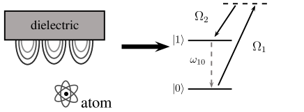
Figure 1: Scheme of resonance between the atomic transition and one surface polariton which leads to the creation of a second polariton $\displaystyle\Omega_{1}\approx\omega_{10}+\Omega_{2}$.

To illustrate our basic idea, we consider the interaction of an atomic transition of frequency $\displaystyle\omega_{10}$ between two eigenstates $\displaystyle|0\rangle$ and $\displaystyle|1\rangle$ with two surface polaritons with corresponding center frequencies $\displaystyle\Omega_{1}$ and $\displaystyle\Omega_{2}$ $\displaystyle(\Omega_{1}\neq\Omega_{2})$ for whom the resonance condition $\displaystyle\Omega_{1}\approx\omega_{10}+\Omega_{2}$ is satisfied. The polariton resonance frequencies $\displaystyle\Omega_{1}$ and $\displaystyle\Omega_{2}$ are assumed to be far from any other atomic transition frequency $\displaystyle\omega_{mn}$.

Heisenberg’s equations of motion $\displaystyle\dot{\hat{O}}=\frac{i}{\hbar}[\hat{H},\hat{O}]$ for the dynamical variables and the atomic transition operators follow from the Hamiltonian (1) as

$$\displaystyle\dot{\hat{\mathbf{f}}}(\mathbf{r},\omega,t)=-i\omega\hat{\mathbf{f}}(\mathbf{r},\omega)+\frac{i}{\hbar}\sum_{k,l}\hat{A}_{kl}\mathbf{d}_{kl}\cdot\bm{G}^{\ast}_{e}(\mathbf{r}_{A},\mathbf{r},\omega)\,,$$ (10)

$$\displaystyle\dot{\hat{A}}_{mn}(t)=i\omega_{mn}\hat{A}_{mn}$$

$$\displaystyle-\frac{i}{\hbar}\sum_{k}\left(\hat{A}_{kn}\mathbf{d}_{km}-\hat{A}_{mk}\mathbf{d}_{nk}\right)\cdot\hat{\mathbf{E}}(\mathbf{r}_{A})\,.$$ (11)

These two equations of motion describe the light atom system, for a full solution one needs to solve the two equations. Formal integration of Eq. (11) yields

$$\displaystyle\hat{A}_{mn}(t)=e^{i\omega_{mn}t}\hat{A}_{mn}-\frac{i}{\hbar}\sum_{k}\int\limits_{0}^{t}dt^{\prime}\>e^{i\omega_{mn}(t-t^{\prime})}$$

$$\displaystyle\times\left[\hat{A}_{kn}(t^{\prime})\mathbf{d}_{km}-\hat{A}_{mk}(t^{\prime})\mathbf{d}_{nk}\right]\cdot\hat{\mathbf{E}}(\mathbf{r}_{A},t^{\prime}),$$ (12)

which, inserted back into the equation of motion for the dynamical variables of the medium-assisted field, Eq. (10), yields the first iteration of the equations of motion for the dynamical variables as

$$\displaystyle\dot{\hat{\mathbf{f}}}(\mathbf{r},\omega,t)=-i\omega\hat{\mathbf{f}}(\mathbf{r},\omega)+\frac{i}{\hbar}\sum_{m,n}e^{i\omega_{mn}t}\hat{A}_{mn}\mathbf{d}_{mn}\cdot\bm{G}^{\ast}_{e}(\mathbf{r}_{A},\mathbf{r},\omega)+\frac{1}{\hbar^{2}}\sum_{k,m,n}\int\limits_{0}^{t}dt^{\prime}\int\limits_{0}^{\infty}d\omega^{\prime}\int d^{3}r^{\prime}\,e^{i\omega_{mn}(t-t^{\prime})}$$

$$\displaystyle\times\mathbf{d}_{mn}\cdot\bm{G}^{\ast}_{e}(\mathbf{r}_{A},\mathbf{r},\omega)\left[\hat{A}_{kn}(t^{\prime})\mathbf{d}_{km}-\hat{A}_{mk}(t^{\prime})\mathbf{d}_{nk}\right]\cdot\left[\bm{G}_{e}(\mathbf{r}_{A},\mathbf{r}^{\prime},\omega^{\prime})\cdot\hat{\mathbf{f}}(\mathbf{r}^{\prime},\omega^{\prime},t^{\prime})+\bm{G}^{\ast}_{e}(\mathbf{r}_{A},\mathbf{r}^{\prime},\omega^{\prime})\cdot\hat{\mathbf{f}}^{\dagger}(\mathbf{r}^{\prime},\omega^{\prime},t^{\prime})\right]\,.$$ (13)

Equation (13) is now a nonlinear operator equation that is capable of describing resonant processes involving two polaritons. This is despite the fact that the original Hamiltonian (1) is bilinear in all operators. The effective nonlinearity appears as a consequence of the iteration. In order to pick out the resonant interactions from the equation of motion, we introduce slowly varying amplitude operators as $\displaystyle\hat{\tilde{\mathbf{f}}}(\mathbf{r},\omega,t)=\hat{\mathbf{f}}(\mathbf{r},\omega,t)e^{i\omega t}$ and $\displaystyle\hat{\tilde{A}}_{mn}(t)=\hat{A}_{mn}(t)e^{-i\omega_{mn}t}$ and apply the Markov approximation. This involves taking the slowly varying amplitude operators out of the integral at the upper time $\displaystyle t$. For simplicity let us demonstrate this for one of the terms in Eq. (13),

$$\displaystyle\mathbf{I}_{1}(\mathbf{r},\omega,t)$$ (14)

$$\displaystyle\equiv\frac{1}{\hbar^{2}}\sum_{k,m,n}\int\limits_{0}^{t}dt^{\prime}\int\limits_{0}^{\infty}d\omega^{\prime}\int d^{3}r^{\prime}\,e^{i\omega_{mn}(t-t^{\prime})}\hat{A}_{kn}(t^{\prime})$$

$$\displaystyle\times\mathbf{d}_{mn}\cdot\bm{G}^{\ast}_{e}(\mathbf{r}_{A},\mathbf{r},\omega)\mathbf{d}_{km}\cdot\bm{G}_{e}(\mathbf{r}_{A},\mathbf{r}^{\prime},\omega^{\prime})\cdot\hat{\mathbf{f}}(\mathbf{r}^{\prime},\omega^{\prime},t^{\prime})$$

$$\displaystyle=\frac{1}{\hbar^{2}}\sum_{k,m,n}\int\limits_{0}^{\infty}d\omega^{\prime}\int d^{3}r^{\prime}\,\mathbf{d}_{mn}\cdot\bm{G}^{\ast}_{e}(\mathbf{r}_{A},\mathbf{r},\omega)\hat{A}_{kn}(t)$$

$$\displaystyle\times\mathbf{d}_{km}\cdot\bm{G}_{e}(\mathbf{r}_{A},\mathbf{r}^{\prime},\omega^{\prime})\cdot\hat{\mathbf{f}}(\mathbf{r}^{\prime},\omega^{\prime},t)\int\limits_{0}^{t}dt^{\prime}e^{i(\omega_{mk}+\omega^{\prime})(t-t^{\prime})}\,.$$

The integrals can be approximated in the long-time limit, i.e. by extending the upper limit of integration to infinity and assuming that the atomic transitions are well away from the field resonances, so that $\displaystyle\int_{0}^{t}dt^{\prime}e^{i(\omega_{mk}+\omega^{\prime})(t-t^{\prime})}\sim-\frac{1}{i(\omega_{mk}+\omega^{\prime})}$. This leads to the result

$$\displaystyle\mathbf{I}_{1}(\mathbf{r},\omega,t)=\frac{1}{\hbar^{2}}\sum_{k,m,n}\int\limits_{0}^{\infty}d\omega^{\prime}\int d^{3}r^{\prime}\,\mathbf{d}_{mn}\cdot\bm{G}^{\ast}_{e}(\mathbf{r}_{A},\mathbf{r},\omega)$$

$$\displaystyle\times\frac{\hat{A}_{kn}(t)\mathbf{d}_{km}\cdot\bm{G}_{e}(\mathbf{r}_{A},\mathbf{r}^{\prime},\omega^{\prime})}{i(\omega_{mk}+\omega^{\prime})}\hat{\mathbf{f}}(\mathbf{r}^{\prime},\omega^{\prime},t).$$ (15)

The other three terms in Eq. (13) can be approximated in an analogous way.

For our present investigation one has to keep in mind that in the nonretarded limit the polariton spectrum is not continuous (see discussion in Sec. III.1) but consists of of a quasidiscrete set of lines of midfrequencies $\displaystyle\Omega_{\nu}$ and widths $\displaystyle\gamma_{\nu}$, where the linewidths are typically very much smaller than the line center separations $\displaystyle\gamma_{\nu}\ll(\Omega_{\nu+1}-\Omega_{\nu-1})/2$. We then divide the $\displaystyle\omega$ axis into intervals $\displaystyle\Delta_{\nu}=[(\Omega_{\nu-1}+\Omega_{\nu})/2,(\Omega_{\nu}+\Omega_{\nu+1})/2]$. Recalling the resonance condition $\displaystyle\Omega_{1}\approx\omega_{10}+\Omega_{2}$, we apply the rotating-wave approximation and finally arrive at the effective equation of motion describing the dynamics of the resonant atom–polariton coupling where now the frequency integrals have to be taken over the linewidth of the surface polaritons,

$$\displaystyle\dot{\hat{\mathbf{f}}}(\mathbf{r},\omega)=-i\omega\hat{\mathbf{f}}(\mathbf{r},\omega)$$

$$\displaystyle-i\int d^{3}r^{\prime}\int\limits_{\Delta_{\nu}}d\omega^{\prime}\,\left[\hat{\mathbf{g}}(\mathbf{r},\mathbf{r}^{\prime},\omega,\omega^{\prime})\cdot\hat{\mathbf{f}}(\mathbf{r}^{\prime},\omega^{\prime})\right]\,.$$ (16)

Here we have introduced the abbreviation

$$\displaystyle\hat{\mathbf{g}}(\mathbf{r},\mathbf{r}^{\prime},\omega,\omega^{\prime})=$$

$$\displaystyle-\frac{\hat{A}_{10}}{\hbar}\sum_{k}\bigg{[}\frac{\mathbf{d}_{k0}\cdot\bm{G}^{\ast}_{e}(\mathbf{r}_{A},\mathbf{r},\omega)\otimes\mathbf{d}_{1k}\cdot\bm{G}_{e}(\mathbf{r}_{A},\mathbf{r}^{\prime},\omega^{\prime})}{\omega_{k1}+\omega^{\prime}}$$

$$\displaystyle-\frac{\mathbf{d}_{1k}\cdot\bm{G}^{\ast}_{e}(\mathbf{r}_{A},\mathbf{r},\omega)\otimes\mathbf{d}_{k0}\cdot\bm{G}_{e}(\mathbf{r}_{A},\mathbf{r}^{\prime},\omega^{\prime})}{\omega_{0k}+\omega^{\prime}}\bigg{]}\,$$ (17)

for the operator-valued coupling tensor. As one can see from the structure of $\displaystyle\hat{\mathbf{g}}(\mathbf{r},\mathbf{r^{\prime}},\omega,\omega^{\prime})$, the atom–polariton coupling is mediated by a virtual atomic transition from $\displaystyle\left|1\right\rangle\rightarrow\left|0\right\rangle$ via an intermediate state $\displaystyle\left|k\right\rangle$ (see Fig. 2) with dipole moments $\displaystyle\mathbf{d}_{1k}$ and $\displaystyle\mathbf{d}_{0k}$.

Figure 2: The transition from $\displaystyle\left|1\right\rangle$ to $\displaystyle\left|0\right\rangle$ is mediated by the virtual transitions via the state $\displaystyle\left|k\right\rangle$.

The equation of motion (13) can be thought of as being generated by the effective second order interaction Hamiltonian

$$\dot{\hat{\mathbf{f}}}=(i\hbar)^{-1}[\hat{\mathbf{f}},\hat{H}_{F}+\hat{H}_{\mathrm{(int)eff}}]\,,$$ (18)

where

$$\displaystyle\hat{H}_{\mathrm{(int)eff}}=\hbar\int d^{3}r^{\prime}\int d^{3}r\int\limits_{\Delta_{\nu}}d\omega\int\limits_{\Delta_{\nu^{\prime}}}d\omega^{\prime}\,$$

$$\displaystyle\hat{\mathbf{f}}^{\dagger}(\mathbf{r},\omega)\cdot\bigl{[}\hat{\mathbf{g}}(\mathbf{r},\mathbf{r}^{\prime},\omega,\omega^{\prime})-\hat{\mathbf{g}}^{\dagger}(\mathbf{r},\mathbf{r}^{\prime},\omega,\omega^{\prime})\bigr{]}\cdot\hat{\mathbf{f}}(\mathbf{r}^{\prime},\omega^{\prime})\,.$$ (19)

This Hamiltonian describes the effective creation of one polariton excitation with a simultaneous annihilation of another. In the specific scenario depicted in Fig. 1, only the term involving $\displaystyle\hat{\mathbf{g}}(\mathbf{r},\mathbf{r}^{\prime},\omega,\omega^{\prime})$ will contribute to the near-resonant interaction Hamiltonian.

III.1 Coupling to singly excited polaritons

We consider an atom at nonretarded distance $\displaystyle z$ from a flat surface of multi–resonance Drude–Lorentz permittivity

$$\varepsilon(\omega)=1+\sum_{j}\frac{\omega_{Pj}^{2}}{\omega_{Tj}^{2}-\omega^{2}-i\omega\Gamma_{j}}$$ (20)

with plasma frequencies $\displaystyle\omega_{Pj}$ and transverse resonance frequencies $\displaystyle\omega_{Tj}$. The Green tensor for a half-infinite dielectric medium (subscript $\displaystyle d$) in vacuum (subscript $\displaystyle v$) can be given as

$$\displaystyle\mathbf{G}(\mathbf{r},\mathbf{r},\omega)=\frac{i}{8\pi}\int_{0}^{\infty}dk_{\rho}\frac{k_{\rho}}{k_{vz}}e^{2ik_{vz}z_{A}}\left\{r_{s}(\omega)\begin{pmatrix}1&0&0\\ 0&1&0\\ 0&0&0\end{pmatrix}\right.$$

$$\displaystyle\left.+r_{p}(\omega)\frac{c^{2}}{\omega^{2}}\begin{pmatrix}-k_{vz}^{2}&0&0\\ 0&-k_{vz}^{2}&0\\ 0&0&2k_{\rho}^{2}\end{pmatrix}\right\}$$ (21)

where

$$\displaystyle r_{p}(\omega)=\frac{\varepsilon(\omega)k_{vz}-k_{dz}}{\varepsilon(\omega)k_{vz}+k_{dz}},r_{s}(\omega)=\frac{k_{vz}-k_{dz}}{k_{vz}+k_{dz}}$$ (22)

are the Fresnel reflection coefficients for $\displaystyle s-$ and $\displaystyle p-$polarized waves. In the nonretarded limit the approximation $\displaystyle k_{vz}=k_{dz}=ik_{\rho}$ can be made and the Green tensor of such a surface reduces to $\displaystyle\bm{G}(\mathbf{r},\mathbf{r},\omega)\simeq z^{-3}\bm{G}^{\prime}(\omega)$ with

$$\bm{G}^{\prime}(\omega)=\frac{c^{2}}{32\pi\omega^{2}}\tilde{r}_{p}(\omega)\begin{pmatrix}1&0&0\\ 0&1&0\\ 0&0&2\end{pmatrix}$$ (23)

where now $\displaystyle\tilde{r}_{p}(\omega)=(\varepsilon(\omega)-1)/(\varepsilon(\omega)+1)$. The general condition to obtain $\displaystyle p-$polarized surface waves is given by the dispersion relation

$$\varepsilon(\omega)k_{vz}+k_{dz}=0\,.$$ (24)

When taken to the nonretarded limit ($\displaystyle k\to\infty$) it exhibits resonances where the associated modes are the surface polaritons (strictly speaking, there are poles in the complex frequency plane where $\displaystyle\varepsilon(\omega)=-1$).

Combining these two equations, one sees that the local density of states $\displaystyle\omega^{2}\mathrm{Im}\,\bm{G}(\mathbf{r},\mathbf{r},\omega)$ near a given polariton resonance can be approximated by a single Lorentzian peak of mid-frequency $\displaystyle\Omega_{\nu}$ and width $\displaystyle\gamma_{\nu}$,

$$\omega^{2}\mathrm{Im}\,\bm{G}(\mathbf{r},\mathbf{r},\omega)\simeq\Omega_{\nu}^{2}\mathrm{Im}\,\bm{G}(\mathbf{r},\mathbf{r},\Omega_{\nu})\frac{\gamma_{\nu}^{2}/4}{(\omega-\Omega_{\nu})^{2}+\gamma_{\nu}^{2}/4}\,.$$ (25)

It is then useful to define the respective single–polariton excitations (similar to the generic construction of quantum-mechanical single-photon wave packets, cf. Ref. Buhmann and Welsch (2008)) as

$$\displaystyle\left|1(\mathbf{r}_{A},\Omega_{i})\right\rangle=\sqrt{\frac{2}{\pi\gamma_{i}}}\int\limits_{\Delta_{\Omega_{i}}}d\omega\int d^{3}s\,\frac{1}{g(\mathbf{r}_{A},\Omega_{i})}$$

$$\displaystyle\times\bm{G}^{\ast}_{e}(\mathbf{r}_{A},\mathbf{s},\omega)\cdot\hat{\mathbf{f}}^{\dagger}(\mathbf{s},\omega)\left|\left\{0\right\}\right\rangle$$ (26)

with the normalization factor

$$g(\mathbf{r}_{A},\Omega_{i})=\sqrt{\frac{\mu_{0}}{\hbar\pi}\Omega_{i}^{2}\mathrm{Tr}\,\mathrm{Im}\,\bm{G}(\mathbf{r}_{A},\mathbf{r}_{A},\Omega_{i})}\,,$$ (27)

where $\displaystyle\mathrm{Tr}$ denotes the trace. Using the integral relation (9) for the Green tensor, the integral in frequency can be approximated in the long–frequency limit by extending the upper limit of integration to infinity using the definition for normalization of a Lorentzian function

$$\int_{-\infty}^{\infty}\frac{1}{\pi}\frac{\gamma/2}{(\omega-\Omega)^{2}+\gamma^{2}/4}=1,$$ (28)

one easily checks that the states (26) are indeed properly normalized, $\displaystyle\langle 1(\mathbf{r}_{A},\Omega_{i})\left|1(\mathbf{r}_{A},\Omega_{i})\right\rangle=1$. Note that the states $\displaystyle\left|1(\mathbf{r}_{A},\Omega_{i})\right\rangle$ carry a vector index as well as the continuous space and frequency labels.

In our envisaged situation of a resonant coupling between a single atomic transition and the difference between two polariton resonances, the energies of the initial and final states are identical. Degenerate first-order perturbation theory asserts that the interacting potential is Cohen-Tannoudji et al. (1997)

$$U_{\mathrm{eff}}=\sqrt{\left|\left\langle K\right|\hat{H}_{\mathrm{eff}}\left|I\right\rangle\right|^{2}}.$$ (29)

Here $\displaystyle\left|I\right\rangle=\left|1_{A}\right\rangle\left|0_{1}\right\rangle\left|1_{2}\right\rangle$ stands for the tensor product of the initial excited atomic state $\displaystyle\left|1_{A}\right\rangle$ and a singly excited polariton with frequency $\displaystyle\Omega_{2}$, and $\displaystyle\left|K\right\rangle=\left|0_{A}\right\rangle\left|1_{1}\right\rangle\left|0_{2}\right\rangle$ denotes the tensor product of the final atomic state $\displaystyle\left|0_{A}\right\rangle$ and a single excitation in the polariton with frequency $\displaystyle\Omega_{1}$. The single-polariton states $\displaystyle\left|1_{\nu}\right\rangle\equiv\left|1(\mathbf{r}_{A},\Omega_{\nu})\right\rangle$ are defined according to Eq. (26) and $\displaystyle\left|0_{\nu}\right\rangle$ denotes the polariton ground state $\displaystyle\left|0_{\nu}\right\rangle=\left|\{0\}\right\rangle$, $\displaystyle\forall\omega\in[\Omega_{\nu}-\delta\omega/2,\Omega_{\nu}+\delta\omega/2]$.

Using the commutation rules of the operators as well as the properties of the Green functions, together with the definition of the Lorentzian lineshape, Eq. (25), we find that the effective interaction potential can be written in the form

$$\displaystyle U_{\mathrm{eff}}=-\frac{\mu_{0}\Omega_{1}\Omega_{2}}{2}$$

$$\displaystyle\times\sqrt{\frac{\gamma_{1}\gamma_{2}}{\mathrm{Tr}\left[\mathrm{Im}\bm{G}(\mathbf{r}_{A},\mathbf{r}_{A},\Omega_{1})\right]\mathrm{Tr}\left[\mathrm{Im}\bm{G}(\mathbf{r}_{A},\mathbf{r}_{A},\Omega_{2})\right]}}$$

$$\displaystyle\sum_{k}\Bigg{\{}\mathrm{Tr}\left[\mathrm{Im}\bm{G}(\mathbf{r}_{A},\mathbf{r}_{A},\Omega_{1})\cdot\mathbf{d}_{0k}\otimes\mathbf{d}_{k1}\cdot\mathrm{Im}\bm{G}(\mathbf{r}_{A},\mathbf{r}_{A},\Omega_{2})\right]$$

$$\displaystyle\times\frac{\Omega_{1}+\omega_{0k}}{(\Omega_{1}+\omega_{0k})^{2}+\gamma_{1}^{2}/4}$$

$$\displaystyle-\mathrm{Tr}\left[\mathrm{Im}\bm{G}(\mathbf{r}_{A},\mathbf{r}_{A},\Omega_{1})\cdot\mathbf{d}_{k1}\otimes\mathbf{d}_{0k}\cdot\mathrm{Im}\bm{G}(\mathbf{r}_{A},\mathbf{r}_{A},\Omega_{2})\right]$$

$$\displaystyle\times\frac{\Omega_{1}+\omega_{k1}}{(\Omega_{1}+\omega_{k1})^{2}+\gamma_{1}^{2}/4}\Bigg{\}}.$$ (30)

Let us compare Eq. (30) with the nonresonant Casimir–Polder potential at finite temperature Scheel and Buhmann (2008); Crosse et al. (2010),

$$\displaystyle\Delta E^{\mathrm{NR}}=\mu_{0}k_{B}T\sideset{}{{}^{\prime}}{\sum}_{j=0}^{\infty}\xi_{j}^{2}\mathrm{Tr}\left[\bm{\alpha}(i\xi_{j})\cdot\bm{G}(\mathbf{r}_{A},\mathbf{r}_{A},i\xi_{j})\right]$$

$$\displaystyle+\mu_{0}\sum_{k\neq n}\omega_{kn}^{2}\bar{n}_{\mathrm{th}}(\omega_{kn})\mathbf{d}_{nk}\cdot\mathrm{Re}\,\bm{G}(\mathbf{r}_{A},\mathbf{r}_{A},\omega_{kn})\cdot\mathbf{d}_{kn},$$ (31)

where $\displaystyle\xi_{j}$ are the Matsubara frequencies, $\displaystyle\bm{\alpha}(\omega)$ is the atomic polarizability and $\displaystyle\bar{n}_{\mathrm{th}}(\omega)=[\exp(\hbar\omega/k_{B}T)-1]^{-1}$ the thermal occupation number. We note that the effective potential scales with the atom-surface distance $\displaystyle z$ in exactly the same way as nonresonant Casimir–Polder potential ($\displaystyle\propto z^{-3}$). The effective Hamiltonian (19) is quadratic in the field variables and contributes to the potential (29) at (degenerate) first-order perturbation theory. The nonresonant potential arises from a Hamiltonian which is linear in the field variables, contributing only in second-order perturbation theory Scheel and Buhmann (2008). In both cases, we therefore obtain a result that is quadratic in the atom-field coupling, or, equivalently, linear in the imaginary part of the Green tensor (the local mode density).

The total potential experienced by the atom is the sum of the nonresonant (attractive) Casimir–Polder potential and the resonant coupling between the atoms and the surface polaritons,

$$\Delta E^{\mathrm{Total}}=\Delta E^{\mathrm{NR}}+\Delta E^{\mathrm{R}}.$$ (32)

Using Eqs. (23) and (25), the respective energy shifts for the nonresonant and (second-order) resonant interactions in the nonretarded limit considering an isotropic atom are

$$\displaystyle\Delta E^{\mathrm{NR}}=-\frac{\mu_{0}c^{2}k_{B}T}{12\pi\hbar z^{3}}\sum_{k}\left|\mathbf{d}_{nk}\right|^{2}\sideset{}{{}^{\prime}}{\sum}_{j=0}^{\infty}\frac{\omega_{kn}}{\omega_{kn}^{2}+\xi_{j}^{2}}\frac{\varepsilon(i\xi_{j})-1}{\varepsilon(i\xi_{j})+1}$$

$$\displaystyle+\frac{\mu_{0}c^{2}}{24\pi z^{3}}\sum_{k}\bar{n}_{\mathrm{th}}(\omega_{kn})\left|\mathbf{d}_{nk}\right|^{2}\mathrm{Re}\left[\frac{\varepsilon(\omega_{kn})-1}{\varepsilon(\omega_{kn})+1}\right]$$ (33)

and

$$\displaystyle\Delta E^{\mathrm{R}}=-\frac{\mu_{0}\Omega_{1}\Omega_{2}}{2z^{3}}\sqrt{\frac{\gamma_{1}\gamma_{2}}{\mathrm{Tr}\left[\mathrm{Im}\bm{G}^{\prime}(\Omega_{1})\right]\mathrm{Tr}\left[\mathrm{Im}\bm{G}^{\prime}(\Omega_{2})\right]}}$$

$$\displaystyle\times\sum_{k}\Bigg{\{}\mathrm{Tr}\left[\mathrm{Im}\bm{G}^{\prime}(\Omega_{1})\cdot\mathbf{d}_{0k}\otimes\mathbf{d}_{k1}\cdot\mathrm{Im}\bm{G}^{\prime}(\Omega_{2})\right]$$

$$\displaystyle\times\frac{\Omega_{1}+\omega_{0k}}{(\Omega_{1}+\omega_{0k})^{2}+\gamma_{1}^{2}/4}$$

$$\displaystyle-\mathrm{Tr}\left[\mathrm{Im}\bm{G}^{\prime}(\Omega_{1})\cdot\mathbf{d}_{k1}\otimes\mathbf{d}_{0k}\cdot\mathrm{Im}\bm{G}^{\prime}(\Omega_{2})\right]$$

$$\displaystyle\times\frac{\Omega_{1}+\omega_{k1}}{(\Omega_{1}+\omega_{k1})^{2}+\gamma_{1}^{2}/4}\Bigg{\}},$$ (34)

recall Eq. (23).

III.2 Thermal States

As we are dealing with thermally excited surface polaritons the concept of perturbation theory has to be expanded from pure states described by a single state vector to a statistical mixture or ensemble of states Fano (1957). The density matrix for a thermal state with temperature $\displaystyle T$ can be written in the Fock basis $\displaystyle|n\rangle$ as

$$\hat{\rho}_{\mathrm{th}}=\sum_{n}p_{n}\left|n\right\rangle\left\langle n\right|=\sum_{n}\frac{e^{-n\hbar\Omega_{n}/k_{B}T}}{Z(T)}\left|n\right\rangle\left\langle n\right|$$ (35)

where $\displaystyle Z(T)=\sum_{m}e^{-m\hbar\Omega_{m}/k_{B}T}$ denotes the partition function.

So far we have computed the interaction energy for the situation in which there is initially only one excited polariton with frequency $\displaystyle\Omega_{2}$ and in the final state only one polariton with frequency $\displaystyle\Omega_{1}$ [see Eq. (29)]. This has to be generalized to thermal states in which there can be initially $\displaystyle m$ polaritons with frequency $\displaystyle\Omega_{1}$ and $\displaystyle n$ polaritons with frequency $\displaystyle\Omega_{2}$. In this case, we rewrite the result of the perturbation theory as

$$\left|\left\langle K\right|\hat{H}_{\mathrm{eff}}\left|I\right\rangle\right|^{2}=\mathrm{Tr}\left[\hat{H}_{\mathrm{eff}}\hat{\rho}_{\mathrm{in}}\hat{H}_{\mathrm{eff}}\left|K\right\rangle\left\langle K\right|\right]$$ (36)

where

$$\displaystyle\hat{\rho}_{\mathrm{in}}=\hat{\rho}_{\mathrm{th}}(\Omega_{1})\otimes\hat{\rho}_{\mathrm{th}}(\Omega_{2})\otimes\left|1_{A}\right\rangle\left\langle 1_{A}\right|$$

$$\displaystyle=\sum_{n,m}p_{m}^{(1)}p_{n}^{(2)}\left|m_{1},n_{2}\right\rangle\left\langle m_{1},n_{2}\right|\otimes\left|1_{A}\right\rangle\left\langle 1_{A}\right|.$$ (37)

Due to the form of the effective interaction Hamiltonian $\displaystyle\hat{H}_{\mathrm{(int)eff}}\propto\hat{\mathbf{f}}^{\dagger}(\mathbf{r},\omega)\hat{\mathbf{f}}(\mathbf{r}^{\prime},\omega^{\prime})$ the only final state $\displaystyle\left|K\right\rangle$ that provides a non-vanishing matrix element will be $\displaystyle\left|K\right\rangle=\left|(m+1)_{1},(n-1)_{2}\right\rangle\left|0_{A}\right\rangle$. Recall that $\displaystyle\hat{\mathbf{f}}\left|k\right\rangle=\sqrt{k}\left|k-1\right\rangle$ and $\displaystyle\hat{\mathbf{f}}^{\dagger}\left|k\right\rangle=\sqrt{k+1}\left|k+1\right\rangle$. Hence,

$$\displaystyle\left|\left\langle K\right|\hat{H}_{\mathrm{eff}}\left|I\right\rangle\right|^{2} \displaystyle= \displaystyle\sum_{m,n}p_{m}^{(1)}p_{n}^{(2)}(m+1)_{(1)}(n)_{(2)}U_{\mathrm{eff}}^{2}$$ (38)

$$\displaystyle= \displaystyle\left[\bar{n}_{\mathrm{th}}(\Omega_{1})+1\right]\bar{n}_{\mathrm{th}}(\Omega_{2})U_{\mathrm{eff}}^{2}.$$

Finally, the resonant energy shift $\displaystyle\Delta E^{R}$ for thermal states will be given as

$$\Delta E^{\mathrm{R}}=U_{\mathrm{eff}}\sqrt{\left[\bar{n}_{\mathrm{th}}(\Omega_{1})+1\right]\bar{n}_{\mathrm{th}}(\Omega_{2})}.$$ (39)

This result is intuitively clear, as the initial polariton with frequency $\displaystyle\Omega_{2}$ has to be thermally populated before the resonant interaction can take place.

III.3 Discussion

Let us apply the general results for the potentials (33) and (39) with (34) to the envisaged Drude–Lorentz model (20). For this scenario with two well-separated narrow polariton resonances, (in this case the width of the polariton resonance $\displaystyle\gamma$ is approximately the same as the width of the Drude-Lorentz resonance $\displaystyle\Gamma$ of the material), the effective potential becomes

$$\displaystyle\Delta E^{\mathrm{R}}\sim-\frac{\mu_{0}c^{2}}{128\pi z^{3}}\frac{\omega_{P1}\omega_{P2}}{\sqrt{\Omega_{1}\Omega_{2}}}$$

$$\displaystyle\times\sqrt{\left[\bar{n}_{\mathrm{th}}(\Omega_{1})+1\right]\bar{n}_{\mathrm{th}}(\Omega_{2})}\sum_{k}\frac{5\left|\mathbf{d}_{0k}\right|\left|\mathbf{d}_{k1}\right|}{12}$$

$$\displaystyle\times\Bigg{\{}\frac{\Omega_{1}+\omega_{0k}}{(\Omega_{1}+\omega_{0k})^{2}+\gamma_{1}^{2}/4}-\frac{\Omega_{1}+\omega_{k1}}{(\Omega_{1}+\omega_{k1})^{2}+\gamma_{1}^{2}/4}\Bigg{\}}.$$ (40)

Similarly, the nonresonant Casimir–Polder potential for a one-polariton model is

$$\displaystyle\Delta E^{\mathrm{NR}}\sim-\frac{\mu_{0}c^{2}}{48\pi z^{3}}\frac{k_{B}T}{\hbar}\sum_{\nu}\frac{\omega_{P}^{2}\left|\mathbf{d}_{1\nu}\right|^{2}}{\Omega\omega_{\nu 1}}$$

$$\displaystyle+\frac{\mu_{0}c^{2}}{24\pi z^{3}}\sum\limits_{\nu}\bar{n}_{\mathrm{th}}(\omega_{\nu 1})\left|\mathbf{d}_{1\nu}\right|^{2}$$

$$\displaystyle\times\mathrm{Re}\left[\frac{\omega_{P}^{2}}{2(\omega_{T}^{2}-\omega_{1\nu}^{2}-i\omega_{1\nu}\Gamma)+\omega_{P}^{2}}\right].$$ (41)

For typical cell materials such as sapphire Yu et al. (2004) and quartz Spitzer and Kleinman (1961) the resonant second order shift was evaluated numerically for atoms typically used in these type of experiments such as Rubidium. For the temperatures at which these experiments are performed, from 350–600 K, the surface polaritons frequencies are thermally populated. In comparison to the nonresonant CP shift (which is in the order of several GHz for Rydberg atoms) the resonant second order shift is too small (only several kHz) to be relevant. Although we have detailed experimental results in Ref. Kübler et al. (2010), a comparison between theory and the experimental work cannot be performed because we lack information on the real cell material properties.

Let us investigate which intermediate atomic transitions might provide the largest second order effect. In order to have an effect that is comparable to then nonretarded Casimir–Polder interaction, there has to be a matching atomic transition between energetically close states — note that the transition $\displaystyle\left|1\right\rangle\to\left|0\right\rangle$ does not need to be allowed by the selection rules — i.e. the intermediate state $\displaystyle\left|k\right\rangle$ has to be close to the initial and final states $\displaystyle\left|1\right\rangle$ and $\displaystyle\left|0\right\rangle$, see Fig. 2. The reason for this constraint is the rapidly decreasing magnitude of the dipole transition matrix element between states with increasing energy difference. Therefore, the dominant contribution will come from an intermediate state $\displaystyle\left|k\right\rangle$ approximately halfway between the initial and final states.

In this case the difference between the resonant and nonresonant terms will come from the last line in Eq. (40). Its maximum value is obtained whenever $\displaystyle\omega_{0k}$ or $\displaystyle\omega_{1k}$ is one of $\displaystyle\Omega_{1}\pm\gamma_{1}/2$; away from these points the numerical value of this term decreases. As we have assumed throughout our calculations that all atomic transitions are far from any single-polariton resonance, the Lorentzian peaks have to be broad, i.e. $\displaystyle\gamma_{1}$ has to be large. This in turn means that, in order for this second order effect to be comparable to the nonresonant Casimir–Polder potential, a strongly dissipative material is needed. Note that we assumed in our derivation that linewidths need to smaller than the line center separations which does not exclude the possibility of the peaks to be broad, in fact that is a characteristic that one observes in real polariton spectra.

With these considerations in mind, we give some estimates to show that it would possible to access this phenomenon. For our purpose we choose the $\displaystyle 27S_{1/2}\to 26S_{1/2}$ transition in rubidium. In order for the second-order process to be relevant, one has to find a material with surface polariton frequencies whose difference matches that atomic transition ($\displaystyle\sim 17$ cm^-1). For example, let us choose a material with surface polaritons at 73 and 90 cm^-1 (which we model as two narrow resonances with $\displaystyle\gamma\sim 0.03\Omega$, in which case $\displaystyle\mathrm{Im}r_{p}(\Omega)>100$). With an atom-surface distance of $\displaystyle z=1\mu$m, the Casimir–Polder shift due to the second-order process is $\displaystyle\Delta E^{\mathrm{R}}=-2.74619\times 10^{7}s^{-1}$. As the total level shift can be calculated to be $\displaystyle\Delta E^{\mathrm{Total}}=-1.07583\times 10^{8}s^{-1}$, the resonant second-order process contributes around $\displaystyle 25\%$ to the todal Casimir–Polder shift and is thus expected to be experimentally accessible.

IV Conclusion

We have shown that second order effective interactions involving two surface polaritons lead to novel contributions to dispersion interactions such as the Casimir-Polder potential. We have explicitly derived the dependence of such effects on the atomic and surface parameters and compared their magnitude to that of the conventional nonresonant Casimir-Polder interaction. In principle, one can envisage conditions under which the two become comparable.

However, a more quantitative analysis is largely dependent on exact data of the individual surface properties. For each dielectric material there is a unique surface polariton spectrum that depends sensitively on the concentration and distribution of the impurities and surface quality of the samples (surface roughness). As each sample is unique, the polariton spectrum should be found experimentally. Current experimental findings have revealed some discrepancies, which are most likely due to variations in the quality of the sample, the degree of its impurities and the orientation of the crystal axes Gorza et al. (2001). The latter effect provides a handle to tune the surface polariton frequency by changing the crystal orientation Failache et al. (1999).

References

• Casimir and Polder (1948) H. B. G. Casimir and D. Polder, Physical Review 73 (1948).
• Scheel and Buhmann (2008) S. Scheel and S. Y. Buhmann, Acta Physica Slovaca 58, 675 (2008).
• Sukenik et al. (1993) C. I. Sukenik, M. G. Boshier, D. Cho, V. Sandoghdar, and E. A. Hinds, Physical Review Letters 70, 560 (1993).
• Reichel and Vuletić (2011) J. Reichel and V. Vuletić, eds., Atom Chips (Wiley-VCH Publication, 2011).
• Gaëtan et al. (2009) A. Gaëtan, Y. Miroshnychenko, T. Wilk, A. Chotia, M. Viteau, D. Comparat, P. Pillet, A. Browaeys, and P. Grangier, Nature Physics Letters 5, 115 (2009).
• Urban et al. (2009) E. Urban, T. A. Johnson, T. Henage, L. Isenhower, D. D. Yavuz, T. G. Walker, and M. Saffman, Nature Physics Letters 5, 110 (2009).
• Gallagher (1988) T. F. Gallagher, Reports in Progress on Physics 51, 143 (1988).
• Crosse et al. (2010) J. A. Crosse, S. A. Ellingsen, K. Clements, S. Y. Buhmann, and S. Scheel, Physical Review A 82, 010901(R) (2010).
• Stehle et al. (2011) C. Stehle, H. Bender, C. Zimmermann, D. Kern, M. Fleischer, and S. Slama, Nature Photonics 5, 494 (2011).
• Shaffer (2011) J. P. Shaffer, Nature Photonics 5, 451 (2011).
• Failache et al. (1999) H. Failache, S. Saltiel, M. Fichet, D. Bloch, and M. Ducloy, Physical Review Letters 83, 5467 (1999).
• Failache et al. (2002) H. Failache, S. Saltiel, A. Fischer, D. Bloch, and M. Ducloy, Physical Review Letters 88, 243603 (2002).
• Kübler et al. (2010) H. Kübler, J. P. Shaffer, T. Baluktsian, R. Löw, and T. Pfau, Nature Photonics 4, 112 (2010).
• Buhmann and Welsch (2008) S. Y. Buhmann and D.-G. Welsch, Physical Review A 77, 012110 (2008).
• Cohen-Tannoudji et al. (1997) C. Cohen-Tannoudji, B. Diu, and F. Laloe, Quantum Mechanics, vol. 2 (Hardcover, Hermann, 1997).
• Fano (1957) U. Fano, Reviews of Modern Physics 29 (1957).
• Yu et al. (2004) G. Yu, N. L. Rowell, and D. J. Lockwood, J. Vac. Sci. Technol. A 22 (2004).
• Spitzer and Kleinman (1961) W. G. Spitzer and D. A. Kleinman, Physical Review 121, 1324 (1961).
• Gorza et al. (2001) M.-P. Gorza, S. Saltiel, H. Failache, and M. Ducloy, The European Physical Journal D 15, 113 (2001).