A two-species continuum model for aeolian sand transport

Abstract

Starting from the physics on the grain scale, we develop a simple continuum description of aeolian sand transport. Beyond popular mean-field models, but without sacrificing their computational efficiency, it accounts for both dominant grain populations, hopping (or “saltating”) and creeping (or “reptating”) grains. The predicted stationary sand transport rate is in excellent agreement with wind tunnel experiments simulating wind conditions ranging from the onset of saltation to storms. Our closed set of equations thus provides an analytically tractable, numerically precise and computationally efficient starting point for applications addressing a wealth of phenomena from dune formation to dust emission.

1 Introduction

Wind-driven sand transport is the most noticeable process shaping the morphology of arid regions on the Earth, Mars and elsewhere. It is responsible for the spontaneous creation of a whole hierarchy of self-organized dynamic structures from ripples over isolated dunes to devastating fields of shifting sands. It also contributes considerably to dust proliferation, which is a major determinant of our global climate. There is thus an urgent need for mathematical models that can efficiently and accurately predict aeolian sand fluxes. But the task is very much complicated by the complex turbulent flow of the driving medium (e.g. streaming air) and the erratic nature of the grain hopping it excites [1]. Yet, it is by now well understood that this hopping of grains accelerated by the wind has some characteristic structure [2]. Highly energetic “saltating” grains make a dominant contribution to the overall mass transport. When impacting on the sand bed, they dissipate some of their energy in a complex process called splash, ejecting a cloud of “reptating” grains [3, 4]. A snapshot of this splash would show a whole ensemble of trajectories corresponding to a distribution of jump lengths from short, over intermediate, to large hops. However, grain-scale studies and theoretical considerations have indicated that a reduced description in terms of only two idealized populations (sometimes called saltons and reptons) should indeed be able to provide a faithful parametrization of the complex aeolian sand transport process and the ensuing structure formation [2, 5]. A rule of thumb to say which grains in a real splash pertain to idealized population of saltating or reptating grains is, whether or not their jump height exceeds a threshold of about a few grain diameters.

A drawback of the two-species description has been that it is still conceptually and computationally quite demanding. For reasons of simplicity and computational efficiency, many theoretical studies have therefore chosen to reduce the mathematical description even further, to mean-field type “single-trajectory” models [6]. This may be justified for certain purposes, e.g. for the mathematical modelling of aeolian sand dunes, which are orders of magnitude larger than the characteristic length scales involved in the saltation process, and thus not expected to be very sensitive to the details on the grain scale. Their formation and migration is thought to predominantly depend on large-scale features of the wind field and of the saltation flux, chiefly the symmetry breaking of the turbulent flow over the dune and the delayed reaction of the sand transport to the wind [7]. Moreover, the reptating grains, although they are many, are generally thought to contribute less to the overall sand transport, because they have short trajectories and quickly get trapped in the bed again. Therefore, it seems admissible to concentrate on the saltating particles. On this basis, numerically efficient models for one effective grain species that can largely be identified with the saltating grain fraction, have been constructed. The Sauermann model [8] is a popular and widely used example of such mean-field continuum models. One-species models have become a very successful means of gaining analytical insight into [9, 10, 11, 12, 13, 14] and to conduct efficient large-scale numerical simulations of [15, 16, 17, 18, 19] the complex structure formation processes caused by aeolian transport. The reduction to a single representative trajectory makes the one-species models analytically tractable and computationally efficient. However, it is also responsible for some weaknesses both concerning the way how the two species are subsumed into one [5] and how they feed back onto the wind [12]. These entail imperfections in the model predictions, most noticeable a systematic overestimation of the stationary flux at high wind speed (see figure 5, below). Therefore, the one-species models have been criticized for their lack of numerical accuracy and internal consistency [5, 20]. There are also a number of interesting phenomena that cannot be quantitatively modelled within a one-species model, because they specifically depend on one of the two species, or on their interaction, or because the two species are not merely conceptually but also physically different.

As three important representatives of such phenomena, we name dust emission from the desert, ripples, and megaripples. Dust is created, exposed to the wind, and emitted by aeolian sand transport, and saltating and reptating particles play quite different roles in these processes [1, 21]. For example, fragmentation processes might be driven by the bombardment of high-energy saltating grains [22], but not by the slower reptating grains. In contrast, the emission of dust hidden from the wind underneath the top layer of grains in a sand bed could arguably be linked to the absolute number of reptating grains dislodged from the bed. The reptating grain fraction and its sensitivity to the local slope of the sand bed are, moreover, held responsible for the spontaneous evolution of aeolian ripples [1, 4, 2, 23, 24, 25, 26, 27, 28, 29]. But the amount of reptating particles depends on the strength of the splash caused by the saltating grains. This interdependence of the reptating and saltating species becomes even more transparent when the two species correspond to visibly different types of grains. This is the case for megaripples, which have wavelengths in the metre range and form on strongly polydisperse sand beds in a process accompanied by a pronounced grain sorting [30, 31, 32]. The mechanism underlying their formation and evolution is still not entirely understood, but it seems that the highly energetic bombardment of small saltating grains drives the creep of the larger grains armouring the ripple crests. The mentioned grain-sorting emerges due to the different hop lengths of the grains of different sizes.

The demand for more faithful descriptions of aeolian sand transport has recently spurred notable efforts to eliminate the deficiencies of the one-species models [11, 12, 33] or to develop a numerically efficient two-species model [5]. It also motivated the development of the model described in detail below, as we felt that the problem has not yet been cured at its root. In our opinion, many of the amendments proposed so far have targeted the symptoms rather than the disease by invoking some ad hoc assumptions. It was our aim to modify the sand transport equations from bottom-up, based on a careful analysis of the physics on the grain scale and including the feedback of the two dissimilar grain populations on the turbulent flow. In this way, we derived a conceptually simple, analytically tractable, and numerically efficient two-species model with only two phenomenological fit parameters. They serve to parametrize the complicated splash process and take very reasonable values if the predicted flux law is fitted to measured data. Compared with the time when the first continuum sand transport models were formulated, we could build on a more detailed experimental and theoretical knowledge of the grain-scale physics [5, 34, 35, 36, 37, 38, 39] and rely on more comprehensive empirical information about the wind shear stress and sand transport to test our predictions [40, 41, 42, 43].

The plan of the paper is as follows. We first summarize some of the pertinent basic notions of turbulent flows and aeolian sand transport and introduce the two-species formalism. Then we implement the two-species physics on the level of the sand flux in section 3.1, and on the level of the turbulent closure for the wind in section 3.2. In sections 3.3 and 3.4, we address the most interesting observables, namely the speed and the average number of hopping grains, and the saturated sand flux. We finally compare our results with other models and experiments in section 4, before concluding in section 5.

2 Basic notions of aeolian sand transport and the two-species parametrization

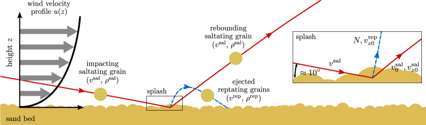
Figure 1: The two-species picture of aeolian sand transport maps the ensemble of mobile grains onto two representative species. High-energy (“saltating”) grains accelerated by the wind (arrows in the wind-speed profile indicating the wind velocity) rebound upon impact and eject some low-energy (“reptating”) grains in a splash. Sand transport is quantified in terms of the transport velocities, $v^{\mathrm{sal}}$ and $v^{\mathrm{rep}}$, and mean densities, $\rho^{\mathrm{sal}}$ and $\rho^{\mathrm{rep}}$, of the two species. The momentum balance of the splash process (inset, see section 3.1) is effectively encoded in the impact velocity $v^{\mathrm{sal}}$, the horizontal and vertical rebound velocities of the saltating grain, $v^{\mathrm{sal}}_{0}$ and $v^{\mathrm{sal}}_{z0}$, respectively, and the number $N$ and velocity $v^{\mathrm{rep}}_{z0}=v^{\mathrm{rep}}_{0}$ of the ejected reptating grains (neglecting a small horizontal velocity component, for simplicity).

Our analysis of the two-phase flow of air and sand is similar, in spirit, to the Sauermann model [8]. The Sauermann model is a continuum or hydrodynamic model. Rather than with the positions and velocities of individual grains it deals with spatio-temporal fields of these quantities, viz. the local mass density $\varrho(\vec{x},t)$ and sand transport velocity $\vec{v}(\vec{x},t)$. It is of mean-field type since it reduces both fields to the mean quantities $\rho(x,t)$, $v(x,t)$ for a single representative trajectory, characterizing the conditions along the wind direction (the $x$-direction), with the distribution of airborne grains in the vertical direction (the $z$-direction) integrated out. Note that $\rho$ therefore is an area density, obtained from integrating the volume density $\varrho$ over $z$. (The vertical grain distribution is a crucial element of the modified turbulent closure, though, which accounts for the feedback of the sand onto the wind.) In this contribution, we deal exclusively with the saturated sand flux, i.e. the sand flux along the wind direction over a flat sand bed and under stationary wind conditions. What we call the flux $q=\rho v$ is actually a vertically integrated flux, or a sand transport rate [8]. The central aim is to derive a constitutive relation $q(\tau)$, giving the stationary flux at a given shear stress $\tau$.

In the following, the strong mean-field approximation of the one-species models is somewhat relaxed and reptating and saltating particles with densities $\rho^{\mathrm{rep}}$, $\rho^{\mathrm{sal}}$ and transport velocities $v^{\mathrm{rep}}$, $v^{\mathrm{sal}}$ are treated separately. The flux is split up accordingly

$$q=q^{\mathrm{rep}}+q^{\mathrm{sal}}=\rho^{\mathrm{sal}}v^{\mathrm{sal}}+\rho^{\mathrm{rep}}v^{\mathrm{rep}}\,.$$ (1)

Introducing the dimensionless mass fraction $\varphi\in[0,1]$ of saltating grains relative to the total amount of mobile grains, the (integrated) densities of the mobile grains can be written in the form

$$\rho^{\mathrm{sal}}=\varphi\rho\quad\mathrm{and}\quad\rho^{\mathrm{rep}}=(1-\varphi)\rho\,.$$ (2)

Accordingly, the flux balance and the relative contribution of reptating and saltating grains to the flux read as

$$\eqalign{q=\rho v=\rho\left[\varphi v^{\mathrm{sal}}+(1-\varphi)v^{\mathrm{rep}}\right]\quad\mathrm{and}\\ q^{\mathrm{rep}}/q^{\mathrm{sal}}=(\varphi^{-1}-1)v^{\mathrm{rep}}/v^{\mathrm{sal}}\,.}$$ (3)

The fluxes depend on the wind velocity field, which, in turn, depends on the grain-wind feedback. To make progress in this respect, the (steady) shear stress $\tau$ in the saltation layer is split up into two components carried by the airborne grains (“g”) and the air (“a”) itself, respectively,

$$\tau=\tau_{\mathrm{g}}(z)+\tau_{\mathrm{a}}(z)=\mathrm{const.}$$ (4)

This idea, introduced by Owen [44], which amounts to an effective two-fluid representation of the wind and the airborne sand, was used in many analytical models [5, 8, 11, 45] and confirmed by numerical simulations [6, 37, 38, 39, 46]. In the two-species model, we moreover keep track of the two species of mobile grains in (4). Similar to the flux division introduced in (1), we further split up the grain-borne shear stress

$$\tau_{\mathrm{g}}(z)=\tau_{\mathrm{g}}^{\mathrm{rep}}(z)+\tau_{\mathrm{g}}^{\mathrm{sal}}(z)\,.$$ (5)

Concerning the feedback of the grains on the wind, it turns out that the wind velocity profile $u(z)$ is predominantly determined by the reptating grain fraction and thus by the functional form of $\tau_{\mathrm{g}}^{\mathrm{rep}}(z)$, while the number and trajectories of the saltating grains hardly affect the wind profile at all. Physically, this makes sense, since the saltating particles form a very disperse gas compared with the dense reptating layer. Also note that the reptating grains, which lose all their momentum upon impact, are responsible for the momentum loss of the flow field. The wind profile may thus be computed in a reduced one-species scheme, as explained in section 3.2 and B.

Under steady conditions, a common simplifying assumption is that the airborne stress near the ground ($z=0$) can be identified with the threshold shear stress $\tau_{\mathrm{t}}$ required to mobilize grains from the ground [44],

$$\tau_{\mathrm{a}}(0)\approx\tau_{\mathrm{t}}\,.$$ (6)

If it were larger or smaller, an increasing or decreasing number of grains would be mobilized, respectively, resulting in an unsteady flow. This idea is indeed supported by empirical observations, which find that the number of ejected grains increases (almost linearly) with the impact speed, not their ejection velocity or jump height [34, 35, 47, 48]. The feedback of the grains on the wind thus essentially fixes the air shear stress at the ground (and, if $\tau\approx\tau_{\mathrm{t}}$, also above) to the threshold value $\tau_{\mathrm{t}}$. To be precise, $\tau_{\mathrm{t}}$ is called the impact threshold, to emphasize that it is easier to lift grains from the splash cloud than to lift completely immobile grains from the ground [1]. But, for the sake of simplicity, we do not bother to make this distinction here, nor do we speculate about possible small deviations of $\tau_{\mathrm{a}}(0)$ from $\tau_{\mathrm{t}}$ under steady conditions [12, 33]. Combining (4) and (6), we may express the shear stress contributed by the grains near the ground as

$$\tau_{\mathrm{g}}(0)=\tau_{\mathrm{g}}^{\mathrm{rep}}(0)+\tau_{\mathrm{g}}^{\mathrm{sal}}(0)=\tau-\tau_{\mathrm{t}}\,.$$ (7)

Both stress contributions are defined as the product of the vertical sand flux $\phi^{i}$ and the horizontal velocity difference $v^{i}-v_{0}^{i}$ upon impact, $\tau_{\mathrm{g}}^{i}(0)=(v^{i}-v_{0}^{i})\phi^{i}$. The vertical sand flux $\phi^{i}$ is given by the horizontal (height integrated) flux $q^{i}$ divided by the grains’ mean hop length, $\phi^{i}\propto q^{i}=\rho^{i}v^{i}$. Here, $i$ represents the species indices “$\mathrm{rep}$” or “$\mathrm{sal}$”. Following Sauermann et al[8], we assume parabolic grain trajectories with initial horizontal and vertical velocity components $v_{0}^{i}$ and $v_{z0}^{i}$, respectively, and obtain

$$\phi^{i}=g\rho^{i}/(2v_{z0}^{i})\,,\quad\tau_{\mathrm{g}}^{i}(0)=g\rho^{i}(v^{i}-v_{0}^{i})/(2v_{z0}^{i})\,,\quad i=\mathrm{rep},\,\mathrm{sal}\,.$$ (8)

Since the average ejection angle of the reptating particles is known to be about $80^{\circ}$ [34], $v_{0}^{\mathrm{rep}}\approx 0$ and we identify the total ejection speed of the reptating grains with its vertical component $v^{\mathrm{rep}}_{z0}$. The impact angle of saltating grains is known to be almost independent of the wind strength and to take typical mean values of about $10^{\circ}$ [49], so that we can identify the total impact speed with the horizontal speed $v^{\mathrm{sal}}$ of the impacting particle, see figure 1.

In order to derive the sought-after constitutive equation, we have to understand the balance of the two species of mobile grains. If one considers the vertical fluxes $\phi^{\mathrm{sal}}$ and $\phi^{\mathrm{rep}}$ rather than the horizontal fluxes $q^{\mathrm{sal}}$ and $q^{\mathrm{rep}}$, one has

$$\phi^{\mathrm{rep}}=N\phi^{\mathrm{sal}}\,,$$ (9)

with the average number $N$ of reptating grains ejected by an impacting saltating grain. Together with the first relation in (8), we then have

$$\varphi^{-1}=1+Nv^{\mathrm{rep}}_{z0}/v^{\mathrm{sal}}_{z0}\,.$$ (10)

Using also the second relation in (8) and remembering that we dismissed the horizontal component of the ejection velocity, we can thus write the overall density of mobile grains in the form

$$\rho=\frac{2\varrho_{\mathrm{air}}}{g}\frac{u_{\ast}^{2}-u_{\ast\mathrm{t}}^{2}}{\varphi(v^{\mathrm{sal}}-v^{\mathrm{sal}}_{0})/v^{\mathrm{sal}}_{z0}+(1-\varphi)v^{\mathrm{rep}}/v^{\mathrm{rep}}_{z0}}\,.$$ (11)

As often found in the literature, we have employed the notion of the shear velocity or friction velocity $u_{\ast}$, defined by $\tau\equiv\varrho_{\mathrm{air}}u_{\ast}^{2}$, as a more intuitive measure of the shear stress $\tau$ here. The velocity ratios in the denominator of (11) are supposedly only very weakly dependent on the wind strength. The first one is recognized as an effective restitution coefficient

$$\alpha\equiv v^{\mathrm{sal}}_{z0}/(v^{\mathrm{sal}}-v^{\mathrm{sal}}_{0})$$ (12)

of the saltating grains [8]. Because of the complexity of the splash process, which makes first-principle quantitative estimates of $\alpha$ forbiddingly complex, we suggest to treat it as a phenomenological fit parameter. We do however provide a reasonable theoretical estimate of the ratio $v^{\mathrm{rep}}/v^{\mathrm{rep}}_{z0}$, based on the trajectory of a vertically ejected grain driven by the wind, in section 3.3 and C. Anticipating the result $v^{\mathrm{rep}}/v^{\mathrm{rep}}_{z0}=0.7(\sigma\nu_{\mathrm{air}}g)^{1/3}/u_{\ast\mathrm{t}}$, we can rewrite the density of the transported sand in the more explicit form

$$\rho=\frac{2\varrho_{\mathrm{air}}}{g}\frac{u_{\ast}^{2}-u_{\ast\mathrm{t}}^{2}}{\varphi/\alpha+0.7(1-\varphi)(\sigma\nu_{\mathrm{air}}g)^{1/3}/u_{\ast\mathrm{t}}}\,.$$ (13)

Here $\nu_{\mathrm{air}}$ denotes the kinematic viscosity of air, and since the grain-air density ratio $\sigma\gg 1$ under terrestrial conditions, we do not bother to distinguish between $\sigma$ and $\sigma-1$ here and in the following. Note that on top of the explicit wind strength dependence of $\rho$ via the numerator, there is an implicit, yet undetermined one via $\varphi$.

In the following, we develop the sought-after “second generation” transport law $q(u_{\ast})$, based on the grain-scale physics. Some empirical input is employed to fix certain phenomenological coefficients summarized in table 2. Our result (see table 1) accounts for essential elements of the aeolian sand transport process beyond the single-trajectory approximation, and turns out to be in remarkable agreement with wind tunnel measurements.

3 Implementing the two-species framework

The two-species framework is implemented in three steps. First, we deal with the mass balance between the species, then with their feedback onto the wind and their resulting transport velocities, before we finally arrive at an improved stationary transport law $q(u_{\ast})$.

3.1 Sand density: two-species mass balance

We first estimate the partition of the grain population into a saltating and a reptating fraction from several evident assumptions for the splash process, based on fundamental physical principles. In our formalism, a saltating grain always rebounds upon impact and ejects $N$ reptating grains, while a certain fraction of its kinetic energy and momentum is dissipated in the sand bed. We further assume that every reptating grain performs only a single hop after which it remains trapped in the sand bed. These mild approximations for the stationary sand transport reduce the number of free parameters of our model compared with more elaborate descriptions [5].

As argued, e.g., by Kok and Renno [37], the relevant constraint limiting the number $N$ of ejected grains per impact is given by the conservation of the grain-borne momentum rather than the energy. In writing the momentum balance, we make a physically plausible linear-response approximation, namely that all terms scale linearly in the velocity $v^{\mathrm{sal}}$ of the impacting grain. This amounts to assuming a wind-strength-independent scattering geometry, so that we can add $z$- and $x$-components up to constant geometric factors that are later absorbed in phenomenological coefficients. Including also the bed losses proportional to $v_{\mathrm{bed}}$ in this vein, we have

$$v^{\mathrm{sal}}=v^{\mathrm{sal}}_{0}+v^{\mathrm{sal}}_{z0}+Nv^{\mathrm{rep}}_{z0}+v_{\mathrm{bed}}\,.$$ (14)

For the first two terms on the right-hand side of (14), the proportionality to $v^{\mathrm{sal}}$ is already implicit in the definition (12) of the restitution coefficient $\alpha$. There is an important subtlety concerning the last two terms, however. Namely, the ejected grains have to gain enough momentum to jump over neighbouring grains in the bed in order to be counted as mobile grains. But they also should not themselves eject other grains upon impact; otherwise we would have to count them among the saltating fraction. Hence, the impact velocity $v^{\mathrm{rep}}$ and the ejection velocity $v^{\mathrm{rep}}_{z0}$ of the reptating grains are tightly constrained and cannot, by definition, be strongly dependent of the impact velocity of the saltating grain or the wind strength. Within experimental errors, observations of the collision process of saltating grains by Rice et al[49] are indeed in reasonable agreement with a constant $v^{\mathrm{rep}}_{z0}$ of the order of $u_{\ast\mathrm{t}}$. In fact, they found the horizontal component of the ejection velocity to be independent of $v^{\mathrm{sal}}$, and only a slight increase of the vertical component with $v^{\mathrm{sal}}$. A compelling confirmation of this observation was recently obtained by better controlled laboratory experiments, in which PVC beads were injected at an impact angle of $10^{\circ}$ onto a quiescent bed of such beads [34, 35]. There are two important consequences of the constraints on $v^{\mathrm{rep}}_{z0}$. Firstly, $N$ should grow linearly with $v^{\mathrm{sal}}$. Secondly, since the momentum of the impacting grain is only partially transferred to the ejected grains, a critical impact velocity $v^{\mathrm{sal}}=v^{\mathrm{sal}}_{\mathrm{c}}\gg v^{\mathrm{rep}}_{z0}$, has to be overcome to mobilize any grains at all. It can be interpreted as a constant offset in $v_{\mathrm{bed}}$, which does not scale with $v^{\mathrm{sal}}$. According to the collision experiments [34, 35], one can take $v^{\mathrm{sal}}_{\mathrm{c}}\approx 40\sqrt{gd}\approx 9u_{\ast\mathrm{t}}$, where we used Bagnold’s estimate $u_{\ast\mathrm{t}}^{2}\approx 0.01\sigma gd$ [1]. A concise summary of the empirical input entering our model is provided in table 2.

Summarizing the above discussion, we can rewrite the momentum balance (14) as

$$Nv^{\mathrm{rep}}_{z0}\propto v^{\mathrm{sal}}-v^{\mathrm{sal}}_{\mathrm{c}}\,,$$ (15)

where $v^{\mathrm{sal}}>v^{\mathrm{sal}}_{\mathrm{c}}$ is tacitly assumed to hold throughout our discussion, and the omitted factor of proportionality should be insensitive to the wind strength. Observations of saltating grains [49], model collision experiments [34, 35, 47, 48], particle dynamics simulations [6, 50] and reduced numerical models, such as the binary collision scheme proposed by Valance and Crassous [36], all support this affine relation of the number of ejected grains, which is the cornerstone of our two-species mass balance. To fix the omitted factor in (15) and make contact with (10), we write

$$Nv^{\mathrm{rep}}_{z0}=(\eta/\alpha)\left(1-v^{\mathrm{sal}}_{\mathrm{c}}/v^{\mathrm{sal}}\right)v^{\mathrm{sal}}_{z0}\,.$$ (16)

The constant $\eta$, which serves as the second free fit parameter of our model, determines together with $v^{\mathrm{sal}}_{\mathrm{c}}$ how the momentum lost by a rebounding grain is distributed between the bed and the ejected particles. (Details of the phenomenological values of $\alpha$ and $\eta$ obtained by fitting the complete model to the experimental flux data are given below.) Comparison with (10) now yields an explicit expression of the mass fraction

$$\varphi^{-1}=1+(1-v^{\mathrm{sal}}_{\mathrm{c}}/v^{\mathrm{sal}})\eta/\alpha$$ (17)

in terms of $v^{\mathrm{sal}}$, alone. Thereby, the problem of specifying the stationary mass balance between saltating and reptating grains has been completely reduced to the task of finding the stationary transport velocity $v^{\mathrm{sal}}$ of the saltating particles as a function of the wind strength.

3.2 Wind velocity field: two-species turbulent closure

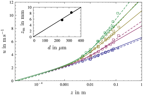
Figure 2: The wind speed $u$ at height $z$. Theory, equation (21) (curves), compared with the measured data (symbols) for grains of diameter $d=242\,\mathrm{\mu m}$ (solid curves, circles) and $d=320\,\mathrm{\mu m}$ (dashed curves, boxes) and various shear velocities ($u_{\ast}=0.27$, $0.39$, $0.56$, $0.69\,\mathrm{m\,s^{-1}}$ and $u_{\ast}=0.27$, $0.47$, $0.74$, $0.87\;\mathrm{m\,s^{-1}}$ from bottom to top for $d=242\;\mathrm{\mu m}$ [42] and $d=320\;\mathrm{\mu m}$ [41], respectively); as global fit parameters we used the roughness length ($z_{0}=d/20$), the threshold shear velocity ($u_{\ast\mathrm{t}}=0.19\;\mathrm{m\,s^{-1}}$, $0.20\;\mathrm{m\,s^{-1}}$ for the finer/coarser sand) and the mean saltation height $z_{\mathrm{m}}$, which is compared with (23) in the inset.

Before we can work out the transport velocities of the two species of grains, we need to know the height-dependent wind speed $u(z)$ and how it is affected by the presence of the airborne grains. Unfortunately, this leads us back to the question of the grain densities that we just delegated to the calculation of the grain velocities. In the past, an elaborate self-consistent calculation has been avoided by anticipating the resulting form of the wind profile on the basis of empirical observations. In the Sauermann model, for instance, an exponential vertical decay of the grain-borne shear stress is imposed,

$$\tau_{\mathrm{g}}(z)=\tau_{\mathrm{g}}(0)\exp(-z/z_{\mathrm{m}})\,,$$ (18)

in good agreement with grain-scale simulations [6, 37, 38, 46]. Since the airborne stress $\tau_{\mathrm{a}}(z)$ follows from this via (4), it reduces the task to the problem of finding the mean saltation height $z_{\mathrm{m}}$. In B, we present a refined version of this approach, adapted to the two-species approach. It accounts for the contributions of the different species to the grain-borne shear stress, separately, and also for their considerably different trajectories. However, as we detail in the appendix, the whole exercise yields essentially identical results as (18), which can in fact be interpreted as the pre-averaged two-species expression. This lends further support to the general form of (18), recommending it as a suitable basis for our further discussion of the two-species model.

From (18), we get, via (4), the wind speed profile $u(z)$ by integrating Prandtl’s turbulence closure

$$\tau_{\mathrm{a}}(z)=\varrho_{\mathrm{air}}\kappa^{2}z^{2}[\partial_{z}u(z)]^{2}\,.$$ (19)

To proceed analytically, we use a modified secant approximation similar to what was proposed by Sørensen [11]. As shown in A, the closure equation then becomes

$$\partial_{z}u\approx\frac{u_{\ast}}{\kappa z}\left[1-(1-u_{\ast\mathrm{t}}/u_{\ast})\rme^{-z/z_{\mathrm{m}}}\right]\,.$$ (20)

Upon integration from the roughness length $z_{0}\ll z_{\mathrm{m}}$, defined by $u(z_{0})=0$, this yields the explicit result [11, 12]

$$u(z)=\frac{u_{\ast}}{\kappa}\ln(z/z_{0})-\frac{u_{\ast}-u_{\ast\mathrm{t}}}{\kappa}[\mathrm{E}_{1}(z_{0}/z_{\mathrm{m}})-\mathrm{E}_{1}(z/z_{\mathrm{m}})]\,,$$ (21)

with the integral exponential $\mathrm{E}_{1}(z)\equiv\int_{z}^{\infty}\!\rmd x\,\rme^{-x}/x$. For small wind speeds $u_{\ast}\to u_{\ast\mathrm{t}}$ ($u_{\ast}\geq u_{\ast\mathrm{t}}$), the usual logarithmic velocity profile is recovered. Inside the saltation layer, a universal asymptotic wind velocity field

$$u(z)\sim\frac{u_{\ast\mathrm{t}}}{\kappa}\ln(z/z_{0})\qquad(z_{0}\lesssim z\ll z_{\mathrm{m}})$$ (22)

emerges, which is independent of the wind strength outside the saltation layer. This rationalizes the convergence of the wind profiles for different wind strengths, found in wind tunnel measurements, without the ad hoc assumption [12] of a debatable focal point [51], which resulted in the prediction of an unphysical negative flux $q(u_{\ast})$ at high wind speeds [12]. A direct comparison of our above prediction for $u(z)$ with wind tunnel data from [41, 42] can be found in figure 2. From these data (available for two grain sizes $d$) we determine the mean saltation height $z_{\mathrm{m}}$. Past attempts to relate $z_{\mathrm{m}}$ to $d$ invoked a new undetermined length scale depending solely on atmospheric properties [52]. However, the results of our fit rather support the simpler (and more natural) linear relation

$$z_{\mathrm{m}}\approx 25d$$ (23)

(right panel of figure 2). This is in line with recent analytical and numerical work [33], albeit possibly with a somewhat different numerical factor dependent on specific model assumptions.

3.3 Transport kinetics: two-species transport velocities

With the wind speed profile $u(z)$ at hand, we can now determine the characteristic stationary transport velocity $v^{\mathrm{sal}}$ of the saltating sand fraction from a standard force-balance argument. We evaluate the wind speed at a characteristic height $z^{\mathrm{sal}}$, at which the fluid drag on the grains is then balanced with the effective bed friction, in the usual way (for a detailed derivation and discussion, see [8, 12]). Namely, the drag force on a volume element of the saltation cloud (the force per mass acting on a single saltating grain times the density $\rho^{\mathrm{sal}}$ of the saltation cloud) is balanced with $\tau_{\mathrm{g}}^{\mathrm{sal}}(0)$. This yields the transport velocity of the saltating sand fraction

$$v^{\mathrm{sal}}=u\!\left(z^{\mathrm{sal}}\right)-v^{\mathrm{sal}}_{\infty}\,,$$ (24)

with the estimate [12, 53]

$$v^{\mathrm{sal}}_{\infty}\approx\frac{\sqrt{\sigma dg/\alpha}}{1.3+41\,\nu_{\mathrm{air}}/\sqrt{\sigma d^{3}g/\alpha}}$$ (25)

for the terminal steady-state relative velocity $u-v^{\mathrm{sal}}$. Formally, $v^{\mathrm{sal}}_{\infty}$ is equal to the settling velocity asymptotically reached by a grain freely falling in air (of kinematic viscosity $\nu_{\mathrm{air}}$ and with grain–air density ratio $\sigma$), with a rescaled gravitational acceleration $g\mapsto g/(2\alpha)$.

We fix the $u_{\ast}$-independent parameter $z^{\mathrm{sal}}$ by the plausible assumption that the splash at the (impact) threshold wind speed $u_{\ast\mathrm{t}}$ dies out, corresponding to $v^{\mathrm{sal}}(u_{\ast}=u_{\ast\mathrm{t}})=v^{\mathrm{sal}}_{\mathrm{c}}$. The underlying physical picture is that it is the splash that keeps the saltation process going, even below the aerodynamic entrainment threshold, because the reptating particles compensate for rebound failures [5]. Accordingly, using (24) with the logarithmic wind field, equation (22), we find that

$$z^{\mathrm{sal}}=z_{0}\,\exp\!\left(\kappa\frac{v^{\mathrm{sal}}_{\mathrm{c}}+v^{\mathrm{sal}}_{\infty}}{u_{\ast\mathrm{t}}}\right)\,.$$ (26)

In C, we use a similar argument to derive the mean reptation velocity, which turns out to be almost independent of the grain size $d$. It can thus be approximated by the constant

$$v^{\mathrm{rep}}\approx 0.7(\sigma\nu_{\mathrm{air}}g)^{1/3}\,,$$ (27)

for most practical purposes. This relation corresponds to a $u_{\ast}$-independent reptation length $2v^{\mathrm{rep}}v^{\mathrm{rep}}_{z0}/g=0.14[\sigma^{5}\nu_{\mathrm{air}}^{2}d^{3}/g]^{1/6}$ in the centimetre range, while the saltation length $2v^{\mathrm{sal}}v^{\mathrm{sal}}_{z0}/g\propto u_{\ast}^{2}/g$ is quadratic in the shear velocity $u_{\ast}$ (see figure 3) and of the order of decimetres [1, 54, 55].

In figure 3, the transport velocities $v^{\mathrm{sal}}$ and $v^{\mathrm{rep}}$ for the two species and the mean velocity $v=\varphi v^{\mathrm{sal}}+(1-\varphi)v^{\mathrm{rep}}$ are plotted over the shear velocity $u_{\ast}$. An important result is that the species-averaged transport velocity $v$ is nearly constant over a broad range of wind strengths. This is consistent with the fundamental assumption on which the model is based, namely that the number of mobilized grains is sensitive to the wind strength, but their overall transport kinetics is not.

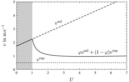
Figure 3: The transport velocities of the saltating (dashed) and reptating (dotted) sand fraction versus the rescaled shear velocity $U\equiv u_{\ast}/u_{\ast\mathrm{t}}$, as predicted by (24) and (27), respectively. The solid line represents the average transport velocity in a reduced effective single-trajectory description.

3.4 Stationary sand flux: two-species transport law

The stationary flux law is now obtained by collecting the above results for the saturated density $\rho$ from (11), the saltation fraction $\varphi$ from (10), the transport velocities (24) with the wind velocity (21), and inserting them into (3). We introduce reduced variables, measuring the shear velocity $u_{\ast}$ in terms of the impact threshold $u_{\ast\mathrm{t}}$ and the saturated flux $q$ in units of $\varrho_{\mathrm{air}}u_{\ast}^{3}/g$,

$$U\equiv u_{\ast}/u_{\ast\mathrm{t}}\,,\qquad Q\equiv qg/(\varrho_{\mathrm{air}}u_{\ast}^{3})\,.$$ (28)

The result for our two-species stationary flux relation then takes the form

$$Q=\left(1-U^{-2}\right)\frac{\alpha_{0}U+\beta_{0}-\gamma_{0}U^{-1}}{aU-b}\,,$$ (29)

with the coefficients $\alpha_{0}$, $\beta_{0}$, $\gamma_{0}$, $a$ and $b$ depending on the two free parameters $\alpha$ and $\eta$, as summarized in D. It goes without saying that this result pertains to $U>1$ and that $Q(U<1)\equiv 0$. Except for $b$, which becomes negative for small $\eta$, and in particular for $\eta=0$, all coefficients are positive. But since $\gamma_{0}<\alpha_{0}+\beta_{0}$ and $b<a$, the flux always remains positive.

The positivity of the flux in (29) guarantees physically reasonable results, even under transient wind conditions, as occurring, for example, in sand dune simulations. The extension of the present discussion to non-stationary conditions is a major task for future investigations, in particular with regard to the saturation length, i.e. the characteristic length scale over which the system relaxes towards the steady state [8]. Its derivation within our two-species approach is of conceptual interest, since the wind strength dependence of the saturation length has recently been the subject of debates (see, e.g., [20]).

4 Discussion

Before we determine the free parameters $\alpha$ and $\eta$ by comparing (29) with experimental data, we first discuss the effect of our two-species parametrization on the two related transport modes—saltation and reptation—and present two different single trajectory reductions of the two-species model. Subsequently, we compare these reduced schemes to single-species transport laws that have previously been proposed in the literature.

4.1 The two-species flux balance

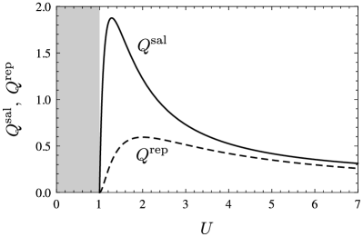
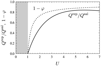
Figure 4: The rescaled fluxes $Q^{\mathrm{sal}}\equiv q^{\mathrm{sal}}g/(\varrho_{\mathrm{air}}u_{\ast}^{3})$ and $Q^{\mathrm{rep}}\equiv q^{\mathrm{rep}}g/(\varrho_{\mathrm{air}}u_{\ast}^{3})$ of the saltating and reptating grains, respectively, versus the rescaled shear velocity $U\equiv u_{\ast}/u_{\ast\mathrm{t}}$ (parameters: $\alpha=0.65$ , $\eta=9$, as determined in section 4.3; grain size $d=250\,\mathrm{\mu m}$). Left: direct comparison of $Q^{\mathrm{sal}}$ (solid line) and $Q^{\mathrm{rep}}$ (dashed line). Right: the flux ratio $Q^{\mathrm{rep}}/Q^{\mathrm{sal}}=q^{\mathrm{rep}}/q^{\mathrm{sal}}$ (solid line) compared with the mass fraction $1-\varphi$ of reptating grains (dashed line).

Our derivation of the overall sand flux $Q$, given in (29), also yields the partial fluxes $Q^{\mathrm{sal}}\equiv q^{\mathrm{sal}}g/(\varrho_{\mathrm{air}}u_{\ast}^{3})$ and $Q^{\mathrm{rep}}\equiv q^{\mathrm{rep}}g/(\varrho_{\mathrm{air}}u_{\ast}^{3})$ of the saltating and reptating species, respectively. Their dependence on the wind velocity is illustrated in figure 4. It is frequently argued in the literature that the saltating grains dominate the sand transport, for they perform large jumps, while the reptating sand fraction might be negligible in terms of mass transport. Our model basically confirms this view for moderate winds, not too far above the impact threshold. However, it predicts that both species contribute almost equally to the total flux, under strong winds. The shift in the mass balance $\varphi$ towards reptation (figure 4, right plot) reflects the dependence of the number of ejected grains on the wind strength, which follows from the splash-impact relation (15) if one inserts the transport velocities of the individual species, as given in figure 3. The variable contribution of the two species to the overall sand flux is a result that cannot be obtained from the conventional single-species models, but should be of interest for some of the more advanced applications mentioned in the introduction.

4.2 One-species limits

Table 1: Scaling functions $f(U)$ for stationary aeolian sand transport relations of the form $Q(U)=\left(1-U^{-2}\right)f(U)$. Note that the coefficients of the various models cannot be identified even if represented by the same symbol. Explicit analytical expressions for the coefficients $\alpha_{0}$, $\beta_{0}$, $\gamma_{0}$, $a$ and $b$ of the two-species model can be found in D.

• This work	$\displaystyle\frac{\alpha_{0}U+\beta_{0}-\gamma_{0}U^{-1}}{aU-b}$
  This work, one-species limit	$\displaystyle a-bU^{-1}$   $(b<0)$
  Sauermann et al2001 [8]	$a\sqrt{1+\alpha_{0}U^{-2}}+bU^{-1}$
  Sørensen 2004 [11]	$a+bU^{-1}+cU^{-2}$
  Durán and Herrmann 2006 [12]	$a-bU^{-1}$   $(a,b<0)$
  Pähtz et al2011 [33]	$-a+bU^{-1}+cU^{-2}$

It is interesting to see how the conventional one-species descriptions emerge from the two-species model upon contraction to a single effective grain species. This contraction is clearly not unique but may be performed in different ways. On the basis of the two-species flux balance, discussed in the preceding section, two natural contractions suggest themselves: one for moderate wind speeds where the flux is dominated by saltation, and one for strong winds, where the ratio of the contributions from reptating and saltating grains was found to be roughly constant.

The first single trajectory reduction, where the reptating species is dismissed, is obtained by setting $\varphi=1$ or $\eta=0$, which corresponds to the flux relation

$$Q=\left(1-U^{-2}\right)\left(a-b\,U^{-1}\right)\,,$$ (30)

with a negative coefficient $b<0$ (D). Since this equation accounts only for high-energy saltating grains, the resulting absolute flux is too large compared with the original two-species description. This can be corrected by reducing the effective trajectory height or, in our formalism, by rescaling the effective height $z^{\mathrm{sal}}$ at which the fluid drag is balanced with the effective bed friction. The lower dotted line in figure 5 was obtained in this way.

The second single trajectory reduction is motivated by the weak dependence of the mass fraction $\varphi$ on $u_{\ast}$ for strong winds $u_{\ast}\gg u_{\ast\mathrm{t}}$, which suggests to replace $\varphi$ by its $u_{\ast}$-independent limit $1/(1+\eta/\alpha)$. This yields

$$Q=\left(1-U^{-2}\right)\left(\tilde{\alpha}_{0}+\tilde{\beta}_{0}\,U^{-1}\right)\,,$$ (31)

with

$$\tilde{\alpha}_{0}=\frac{\alpha_{0}}{a}\quad\mathrm{and}\quad\tilde{\beta}_{0}=\frac{\beta_{0}}{2a}+\frac{\tilde{\eta}}{1+\tilde{\eta}}\frac{v^{\mathrm{rep}}_{z0}}{u_{\ast\mathrm{t}}}\,,$$ (32)

and the abbreviation $\tilde{\eta}\equiv\eta v^{\mathrm{rep}}/v^{\mathrm{rep}}_{z0}$. If one interprets the (now constant) species mass balance as a free phenomenological parameter, it may be adjusted by fine-tuning $\eta$, so that the absolute value of the sand flux predicted by this formula agrees better with experimental observations. This is how we obtained the upper dotted line in figure 5.

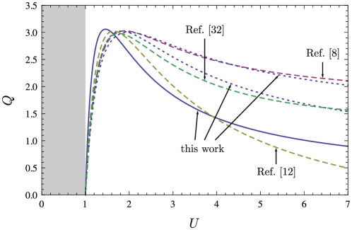
Figure 5: The stationary sand-flux laws. Predictions from the two-species model, equation (29) (solid line) with its natural one-species limits (30) and (31) (lower and upper dotted line), are compared with transport laws from conventional one-species models: Sauermann et al[8] (upper dashed), Durán and Herrmann [12] (lower dashed), and Pähtz et al[33] (middle dashed). All curves have been obtained for a grain size of $d=250\,\mathrm{\mu m}$. The values of the free parameters $\alpha$ and $\eta$ in (29) were determined by comparison to experiments as described in section 4.3. The predictions of the single-trajectory limits of the two-species model, (30) and (31), were adjusted by the parameter rescaling $z^{\mathrm{sal}}\to 0.18z^{\mathrm{sal}}$ and $\eta\to 0.138\eta$.

Both (30) and (31) have the functional form of the transport law proposed by Durán and Herrmann [12] based on the focal point assumption. Note that the effective height $z^{\mathrm{sal}}$ is small compared with the saltation height, where the wind speed obtained from the focal point assumption is very weak. As a consequence, the mean drag force is reduced, which results in a negative parameter $a<0$ in (30) and a negative sand transport rate $Q<0$ for large shear velocities $U>|a/b|$. Table 1 and figure 5 provide a summary of various stationary aeolian sand transport laws that have been proposed in the literature, in comparison with the prediction of our two-species model and its above single-trajectory contractions.

4.3 Comparison with experiments

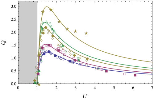
Figure 6: The rescaled saturated flux $Q=qg/(\varrho_{\mathrm{air}}u_{\ast}^{3})$ for various grain sizes ($d=125\,\mathrm{\mu m},\,170\,\mathrm{\mu m},\,242\,\mathrm{\mu m},\,320\,\mathrm{\mu m},\,242\,\mathrm{\mu m}$ from bottom to top): data from wind tunnel measurements using particle tracking methods [43] (stars) and sand traps [40] (other symbols) are compared with the prediction by the two-species model, equation (29) (solid curves). The restitution coefficient $\alpha$ served as a global but grain-size-dependent fit parameter (see figure 7), while $\eta=9$ and $\eta=3.8$ was fixed for the sand trap and the particle tracking data, respectively. (The open symbols represent several rescaled data sets, obtained for a variety of bed slopes.)

We now fit our two-species flux relation $Q(U)$ from (29) to the empirical data from various wind tunnel measurements [40, 43], using $\eta$ and $\alpha$ as free fit parameters. As demonstrated in figure 6, we obtain excellent agreement with the experimental data for a grain-size-independent splash efficiency $\eta$ and an effective coefficient of restitution $\alpha$ that increases with increasing grain size $d$. The transport rates for four different grain sizes collected in [40] were obtained using sand traps; the data in [43] were obtained by particle tracking techniques for a single grain size only. The different methods yield different absolute values for the sand flux, which might be due to systematic differences in the detection efficiency. In the model, these differences are reflected in the (apparently) different efficiencies with which saltating grains generate reptating grains, i.e. different values of the parameter $\eta$. We find that $\eta=3.8$ for the data obtained by particle tracking and $\eta=9$ for the sand trap data, independently of the grain size. But both data sets were consistent with the same formula for the bed restitution coefficient

$$\alpha=1-d_{0}/d\,,$$ (33)

with $d>d_{0}=88\,\mathrm{\mu m}$ (left panel of figure 7). The rebound becomes increasingly elastic for larger grains, while $\alpha$ vanishes for smaller grains at a critical grain diameter $d=d_{0}$, which is in accord with the observation that saltation only occurs for sand grains larger than about $70\,\mathrm{\mu m}$ [56]. The dependence of the restitution coefficient $\alpha$ on the grain size is phyically plausible, for the collision of smaller grains is increasingly influenced by hydrodynamic interactions (and also by cohesive and electrostatic forces). In other words, $d_{0}$ is a characteristic grain size marking the transition from a phenomenology typical of sand to one typical of dust.

Moreover, while we also fine-tune the threshold $u_{\ast\mathrm{t}}$ for each grain size by hand when fitting the experimental data, the values used turn out to be in very good agreement with the expectation $u_{\ast\mathrm{t}}\approx 0.1\sqrt{\sigma gd}$, as demonstrated by the inset of figure 6. Altogether, the stationary sand transport rate observed in experiments is thus convincingly reproduced by the two-species result, equation (29), over a wide parameter range, with very plausible and physically meaningful values for the model parameters.

The observed value of $d_{0}$ can be rationalized by a hydrodynamic order of magnitude estimate. Commonly, one relates the crossover from sand-like to dust-like behaviour to the difference in transport modes of these two classes of granular. While sand is transported by grain hopping dust remains suspended in the air for a while. Balancing the settling velocity of the grains by the typical (upward) eddy currents, which are of the order of $u_{\ast\mathrm{t}}$, one obtains a minimal sand grain size of about $1.5(\nu^{2}/\sigma g)^{1/3}\approx 30\,\mathrm{\mu m}$ [1]. To match $d_{0}=88\,\mathrm{\mu m}$, the eddy velocity would have to be $4.5u_{\ast\mathrm{t}}$. Two further estimates of $d_{0}$ may be obtained as follows. The first assumes that the crossover marked by $d_{0}$ is concomitant with the crossover from a more elastic to a more viscous collision between individual grains. In this case, the relevant quantity is the Stokes number, which characterizes the particle inertia relative to the viscous forces. Using the observations of the collision experiments by Gondret et al[57] for the critical Stokes number $\mathrm{St}$, below which the impacting particles do not rebound from a rigid wall, one gets a critical grain size of about $20\,\mathrm{St}^{2/3}\nu^{2/3}/\sigma/g^{1/3}\approx 20\,\mathrm{\mu m}$. To match $d_{0}=88\,\mathrm{\mu m}$, the critical Stokes number would have to be of the order of 190, i.e. ten times larger than the value obtained in [57], for which experimental differences might possibly be blamed. Note, however, that the most pertinent argument should be the one that gives the largest value of $d_{0}$, as it provides a lower bound for the grain size contributing to saltation. A larger estimate of $d_{0}$ is indeed obtained by observing that sand grains collide with the bed, and they are lifted from the bed by turbulent fluctuations in the wind velocity. In contrast, suspended and resting dust particles are protected from bed collisions and turbulent lift, respectively, by the laminar boundary layer that coats any solid (no slip) boundary. The characteristic length scale of this laminar coating is related to the so-called Kolmogorov dissipation scale $(\nu_{\mathrm{air}}^{3}/\varepsilon)^{1/4}$ [58], where $\varepsilon$ is the dissipation per unit mass of the driving medium (in our case air at normal conditions). For the logarithmic wind profile near the ground, equation (22), the scale-dependent dissipation takes the form $\varepsilon(z)=u_{\ast\mathrm{t}}^{3}/\kappa z$ [59]. A self-consistency argument requiring that the Kolmogorov dissipation scale at height $z$ above the ground equals $z$ (if no externally imposed roughness scale is available) yields $z\simeq[\nu_{\mathrm{air}}^{3}/\varepsilon(d_{0})]^{1/4}$. Extrapolating the logarithmic profile with $u_{\ast\mathrm{t}}=0.1\sqrt{\sigma gd}$ down to the scale $z$, we obtain $z=4.6(\nu_{\mathrm{air}}^{2}/\sigma g)^{1/3}\approx 10^{2}\,\mathrm{\mu m}$. We find this estimate to be in excellent agreement with the data in the left panel of figure 7, which suggests

$$d_{0}\approx 4(\nu_{\mathrm{air}}^{2}/\sigma g)^{1/3}\,.$$ (34)

Figure 7: The restitution coefficient $\alpha$ (left) and the threshold shear velocity $u_{\ast\mathrm{t}}$ (right) versus the grain size $d$. Parameter values deduced from model fits to flux data in figure 6. The solid lines represent the scaling $(d/d_{0})^{-1}$ according to (33) for $1-\alpha$ and the classical estimate $u_{\ast\mathrm{t}}=0.1\sqrt{\sigma gd}$, respectively.

5 Conclusions

We have developed a “second generation” continuum description of aeolian sand transport, relaxing the strong mean-field approximation inherent in the classical single-trajectory models such as [8], and introducing a two-species framework, as advocated in [5]. We started from the physics on the grain scale and corroborated our explicit analytical expressions by a comprehensive comparison with empirical data for the splash, the wind velocity field and the sand flux, covering a broad range of ambient conditions and grain sizes. While the usefulness of our general approach of contracting the complicated splash and saltation process into a drastically reduced two-species picture was strongly suggested by empirical and theoretical work, it necessarily involved some free phenomenological coefficients. For our two-species model, these are, apart from a few minor numerical coefficients listed in table 2, the effective bed restitution coefficient $\alpha(d)$ for the saltating grains of diameter $d$ and the parameter $\eta$ that fixes the number of reptating grains ejected by the average impacting saltating grain. Both parameters were found to take consistent and plausible values if used as free parameters when fitting the empirical flux data obtained in wind tunnel experiments. In particular, the size dependence of the restitution coefficient fits perfectly to the phenomenological criteria commonly used to distinguish dust from sand. The predicted two-species stationary flux law (29) was found to be in excellent agreement with comprehensive data from different sources. It should provide an excellent analytical starting point for a variety of advanced applications calling for a more faithful description of the saltation process so far available—from wind-driven structure formation in the desert to saltation-driven dust production and emission.

Appendix A Solving the Prandtl turbulent closure

With (4) and the assumption of an exponential decay of the grain-borne shear stress with height, equation (18), the modified Prandtl turbulence closure (19) reads as

$$\partial_{z}u=\frac{u_{\ast}}{\kappa z}\sqrt{1-\frac{\tau_{\mathrm{g}}(0)}{\tau}\rme^{-z/z_{\mathrm{m}}}}\,.$$ (35)

To make analytical progress, we follow Sørensen [11] in approximating the square root by a secant. The right-hand side of (35) has the functional form $\sqrt{1-\epsilon x}$, with $x\equiv\exp(-z/z_{\mathrm{m}})$ and $\epsilon\equiv\tau_{\mathrm{g}}(0)/\tau$, which we approximate by a secant of the form $ax+b(1-x)$. Matching the points $\{0,1\}$ and $\{1,\sqrt{1-\epsilon}\}$ yields $b=1$ and $a=\sqrt{1-\epsilon}$, hence

$$\sqrt{1-\epsilon x}\approx 1-(1-\sqrt{1-\epsilon})x\,.$$ (36)

Under stationary conditions, using (7), we have $\sqrt{1-\epsilon}=\sqrt{(\tau-\tau_{\mathrm{g}}(0))/\tau}=u_{\ast\mathrm{t}}/u_{\ast}$, which leads to (20). This avoids an artefact of Sørensen’s original approximation [11], $\sqrt{1-\epsilon x}\approx 1-\epsilon x$, which implies $\sqrt{\tau_{\mathrm{a}}(0)/\tau}=1-\tau_{\mathrm{g}}(0)/\tau$ for the shear stress at the ground, as already criticized by Durán and Herrmann [12].

Appendix B The two-species approach for the wind profile

In (5) of section 2, the grain-borne shear stress was split up into the contributions from saltating and reptating particles, respectively. The ratio of the grain-borne shear stresses at the ground,

$$\frac{\tau_{\mathrm{g}}^{\mathrm{rep}}(0)}{\tau_{\mathrm{g}}^{\mathrm{sal}}(0)}=\alpha\frac{v^{\mathrm{rep}}}{v^{\mathrm{rep}}_{z0}}\frac{1-\varphi}{\varphi}\equiv\tilde{\alpha}\,\frac{1-\varphi}{\varphi}\,,$$ (37)

immediately follows from (8) and (12), and from our simplifying assumption that the reptating grains are ejected vertically. Assuming the exponential decay of the grain-borne shear stress $\tau_{\mathrm{g}}$ with height to hold for both components, the Prandtl turbulent closure reads

$$\rho_{\mathrm{air}}\kappa^{2}z^{2}(\partial_{z}u)^{2}=\tau-\tau_{\mathrm{g}}^{\mathrm{rep}}(0)\rme^{-z/z^{\mathrm{rep}}_{\mathrm{m}}}-\tau_{\mathrm{g}}^{\mathrm{sal}}(0)\rme^{-z/z^{\mathrm{sal}}_{\mathrm{m}}}\,.$$ (38)

We exploit the strong scale separation $z^{\mathrm{sal}}_{\mathrm{m}}/z^{\mathrm{rep}}_{\mathrm{m}}\simeq 10^{2}$ between the characteristic jump heights of saltating and reptating grains [1, 60], on which the two-species model is based. (The precise value turns out to be irrelevant to our discussion.) It allows to solve the closure for two separate height ranges: (i) $z<z^{\mathrm{rep}}_{\mathrm{m}}\ll z^{\mathrm{sal}}_{\mathrm{m}}$associated with reptation, where we may set $\exp(-z/z^{\mathrm{sal}}_{\mathrm{m}})\to 1$, and (ii) $z\gg z^{\mathrm{rep}}_{\mathrm{m}}$, associated with saltation, where we may set $\exp(-z/z^{\mathrm{rep}}_{\mathrm{m}})\to 0$. Applying the secant approximation for the square root as described in A, we can perform the integrations within both ranges and match the asymptotic solutions at $z=z^{\mathrm{rep}}_{\mathrm{m}}$. Using (7) and (37) to eliminate $\tau_{\mathrm{g}}^{\mathrm{sal}}(0)$ and $\tau_{\mathrm{g}}^{\mathrm{rep}}(0)$, this yields

$$u(z)=\cases{\frac{Su_{\ast}}{\kappa}\ln\frac{z}{z_{0}}-\frac{Su_{\ast}-u_{\ast\mathrm{t}}}{\kappa}\left[\mathrm{E}_{1}\!\left(z_{0}/z^{\mathrm{rep}}_{\mathrm{m}}\right)-\mathrm{E}_{1}\!\left(z/z^{\mathrm{rep}}_{\mathrm{m}}\right)\right]\,,&$z\leq z^{\mathrm{rep}}_{\mathrm{m}}$\\ u(z^{\mathrm{rep}}_{\mathrm{m}})+\frac{u_{\ast}}{\kappa}\ln\frac{z}{z^{\mathrm{rep}}_{\mathrm{m}}}\\ \qquad\quad-\frac{u_{\ast}(1-S)}{\kappa}\left[\mathrm{E}_{1}\!\left(z^{\mathrm{rep}}_{\mathrm{m}}/z^{\mathrm{sal}}_{\mathrm{m}}\right)-\mathrm{E}_{1}\!\left(z/z^{\mathrm{sal}}_{\mathrm{m}}\right)\right]\,,&$z>z^{\mathrm{rep}}_{\mathrm{m}}\,,$}$$ (39)

where we abbreviated

$$S=\sqrt{1-\frac{(1-\tau_{\mathrm{t}}/\tau)\varphi}{\varphi+(1-\varphi)\tilde{\alpha}}}\,.$$ (40)

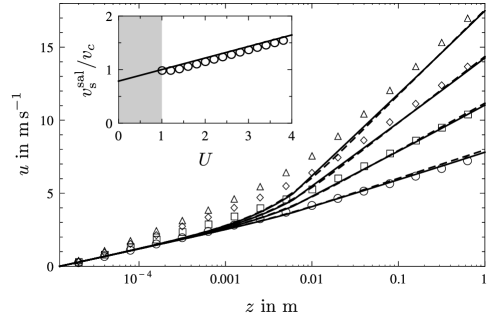
Figure 8: Comparison of the wind velocity profile (39) obtained from the self-consistent numerical solution of (41) (solid lines) with the pre-averaged profile (21) (dashed lines) for grains of diameter $d=242\,\mathrm{\mu m}$ and for various shear velocities ($U=1.5$, 2.5, 3.5 and 4.5 from bottom to top). As explained in the main text, both approaches coincide for $z_{\mathrm{m}}=z^{\mathrm{rep}}_{\mathrm{m}}$. Additionally, we show the results from numerical solutions of the turbulence closure (38) (open symbols) to support the approximate expression (39). Inset: The saltation velocity $v^{\mathrm{sal}}$, rescaled by the minimum saltation velocity $v^{\mathrm{sal}}_{\mathrm{c}}$ needed to eject any grains, over the shear velocity: self-consistent numerical solution of (41) (symbols) and its analytical prediction in the limit $(1-\tau_{\mathrm{t}}/\tau)\varphi\to 0$, for which $u(z)$ is given by (42), (line).

Using this in the force balance, (24), we gain the implicit equation

$$v^{\mathrm{sal}}=u(z^{\mathrm{sal}},v^{\mathrm{sal}})-v^{\mathrm{sal}}_{\infty}\,,$$ (41)

where the fraction $\varphi$ of saltating grains itself depends on the velocity $v^{\mathrm{sal}}$ of the saltating grains via (10). To solve it, we note that the fraction $\varphi$ of saltating particles is a decreasing function of the shear stress $\tau$, bracketed by 1 and 0 (figure 4, right panel). Hence, the product $(1-\tau_{\mathrm{t}}/\tau)\varphi$ is a small number for all $\tau\geq\tau_{\mathrm{t}}$. Setting it to zero in (39), we obtain

$$u(z)\sim\frac{u_{\ast}}{\kappa}\ln\left(\frac{z}{z_{0}}\right)-\frac{u_{\ast}-u_{\ast\mathrm{t}}}{\kappa}\times\cases{[\mathrm{E}_{1}(z_{0}/z^{\mathrm{rep}}_{\mathrm{m}})-\mathrm{E}_{1}(z/z^{\mathrm{rep}}_{\mathrm{m}})]\,,&$z\leq z^{\mathrm{rep}}_{\mathrm{m}}$\\[0.0pt] \,,&$z>z^{\mathrm{rep}}_{\mathrm{m}}$}$$ (42)

Since the exponential integral $\mathrm{E}_{1}(z/z_{\mathrm{m}})$ vanishes rapidly for increasing $z>z_{\mathrm{m}}$, we recover the wind speed profile (21) successfully employed in the one-species models, with the characteristic decay height given by $z_{\mathrm{m}}\equiv z^{\mathrm{rep}}_{\mathrm{m}}$. Inserting (42) into (41) yields an affine increase of $v^{\mathrm{sal}}$ with $u_{\ast}$, in good accord with the exact numerical solution of (41) (figure 8, right panel).

For the numerical solution, one has to deal with the two free parameters $z^{\mathrm{rep}}_{\mathrm{m}}$ and $\alpha$. While the former is directly related to the wind profile, the latter is a fit parameter of the model, determined from a comparison of the predicted sand transport rate with empirical data (figure 6). To make progress, we vary $z^{\mathrm{rep}}_{\mathrm{m}}$ and take the value of $\alpha$ from section 3.4, where the sand flux is estimated by means of the pre-averaged approach for the wind profile. For a grain diameter $d=242\,\mathrm{\mu m}$, we obtained $\alpha\approx 0.63$ (i.e. $\tilde{\alpha}=1.4$), which is consistent with collision experiments, as argued in [12]. From the numerical solution of (41), we find good agreement between the self-consistently gained $u(z)$ and wind tunnel measurements [42] for $z^{\mathrm{rep}}_{\mathrm{m}}=25d$, which is exactly the same value as obtained in section 3.2 within the pre-averaged approach. This supports our observation that (39) can be approximated by taking the limit $\varphi\to 0$ in (42), which yields the pre-averaged wind profile for $z_{\mathrm{m}}\equiv z^{\mathrm{rep}}_{\mathrm{m}}$. This result is almost independent of the ratio $z^{\mathrm{sal}}_{\mathrm{m}}/z^{\mathrm{rep}}_{\mathrm{m}}$, for (42) is independent of $z^{\mathrm{sal}}_{\mathrm{m}}$. Thereby, we formally confirm the intuitive expectation that the feedback of the grains on the wind profile is predominantly due to the many reptating particles and hardly affected by the saltating particles.

Appendix C Reptation velocity

As to the saltating grain fraction in 3.3, we estimate the transport velocity of the reptating grains from the grain-scale physics, i.e. from the hop-averaged horizontal velocity of an individual grain. (Note that we do not introduce a new variable to distinguish the grain-scale velocity from the mean transport velocity, because the context prevents confusion.) The time-dependent velocity of a reptating grain obeys the drag relation

$$\partial_{t}v^{\mathrm{rep}}=\frac{g}{(v^{\mathrm{rep}}_{\infty})^{2}}\,\left|u-v^{\mathrm{rep}}\right|\,\left(u-v^{\mathrm{rep}}\right)\,,$$ (43)

similar to that for saltating grains [8, 12]. For saltating grains, an additional friction force (besides the drag force) would appear on the right-hand site of the equation of motion, representing the mean loss of momentum upon rebound. But, since the reptating grains perform only a single hop, such a friction term does not enter (43). We assume that the ejection is essentially vertical with the initial velocity $v^{\mathrm{rep}}_{z0}$ of the order of $u_{\ast\mathrm{t}}$. A more accurate discussion would not substantially change our findings, as confirmed by the numerical solution of (43). Note that the nonlinearity of the drag law entails a time-dependent “terminal settling velocity” $v^{\mathrm{rep}}_{\infty}$, dependent on the actual relative grain velocity $u-v^{\mathrm{rep}}$ (e.g., [53]). However, for our purpose, and in view of the low reptation trajectories, we can safely approximate the reptation velocity from (43) by inserting the wind speed $u(z^{\mathrm{rep}})$ at a given reptation height and the steady-state terminal velocity

$$v^{\mathrm{rep}}_{\infty}=\sqrt{\sigma gd}\left[0.95+20\,\nu_{\mathrm{air}}/\sqrt{\sigma gd^{3}}\right]^{-1}$$ (44)

derived from the effective drag law proposed in [53], similar to (25) (see also [8, 12]). Neglecting moreover vertical drag forces, the maximum height of the reptation trajectory is $(v^{\mathrm{rep}}_{z0})^{2}/(2g)\approx 10d<z_{\mathrm{m}}$. Consequently, we may insert the ground-level wind field (22) and obtain the mean reptation velocity

$$v^{\mathrm{rep}}\approx\frac{u_{\ast\mathrm{t}}\ln(z^{\mathrm{rep}}/z_{0})}{\kappa\left[1+\kappa\;{(v^{\mathrm{rep}}_{\infty})}^{2}/\left(2v^{\mathrm{rep}}_{z0}u_{\ast\mathrm{t}}\ln(z^{\mathrm{rep}}/z_{0})\right)\right]}\,,$$ (45)

where we approximated the time of flight by that for a parabolic trajectory, $2v^{\mathrm{rep}}_{z0}/g$, as usual. Inserting the empirical observation $v^{\mathrm{rep}}_{z0}\approx u_{\ast\mathrm{t}}$ as well as $u_{\ast\mathrm{t}}^{2}=0.01\sigma gd$ and $z_{0}=d/20$, see table 2, results in an estimate for the reptation velocity $v^{\mathrm{rep}}$ as a function of the grain diameter $d$, illustrated by a solid line in figure 9, which we may identify with the (mean field) transport velocity of the reptating grain fraction.

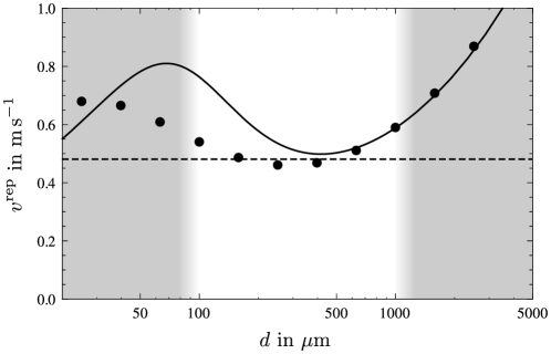
Figure 9: The Reptation velocity $v^{\mathrm{rep}}$ against the grain diameter $d$. The dots correspond to the numerical solution of (43) averaged over one trajectory, while the solid and dashed lines represent the approximate solution (45) and the representative value $v^{\mathrm{rep}}=0.7(\sigma\nu_{\mathrm{air}}g)^{1/3}\approx 0.5\;\mathrm{m\,s^{-1}}$ proposed in (27), respectively. The latter can be understood as an average over the relevant grain sizes (white background).

The yet undetermined value of the effective reptation height $z^{\mathrm{rep}}$ is expected to be of the order of the maximum height $(v^{\mathrm{rep}}_{z0})^{2}/(2g)$ of the trajectory. Indeed, if we compare the approximate result given by (45) with the numerical solution $v^{\mathrm{rep}}(t)$ of (43) averaged over the whole trajectory,

$$\overline{v^{\mathrm{rep}}}=\frac{g}{2v^{\mathrm{rep}}_{z0}}\int_{0}^{2v^{\mathrm{rep}}_{z0}/g}\rmd t\;v^{\mathrm{rep}}(t)\,,$$ (46)

we obtain a good match for large grain diameters $d>800\;\mathrm{\mu m}$ for $z^{\mathrm{rep}}=0.14u_{\ast\mathrm{t}}^{2}/(2g)$. Note, however, that the numerical solution yields an almost $d$-independent reptation velocity $\overline{v^{\mathrm{rep}}}\approx 0.5\;\mathrm{m\,s^{-1}}$ for the relevant grain sizes $d\approx 100\,\mathrm{\mu m}\dots 1\,\mathrm{mm}$, as illustrated in figure 9. To find an estimate for $\overline{v^{\mathrm{rep}}}$, which still captures the dependence on other parameters appearing in (45), we evaluate this equation for a representative grain diameter within the relevant range. A closer look at (45) reveals that the reptation velocity at the inflection point $d\approx 6.7\nu_{\mathrm{air}}^{2/3}(\sigma g)^{-1/3}\approx 150\;\mathrm{\mu m}$ can be approximated by $v^{\mathrm{rep}}\approx(\nu_{\mathrm{air}}\sigma g)^{1/3}=0.68\;\mathrm{m\,s^{-1}}$, which provides the wanted parameter dependence. To better match the absolute values found from the numerical solution, we insert a factor $0.7$ by hand, thus arriving at the analytical estimate given in (27).

Appendix D The coefficients of the transport law

Table 2: The Parameters occurring in equations (47) to (51) which are either numerical constants or dependent on the grain diameter $d$, the gravitational acceleration $g=9.81\;\mathrm{m\,s^{-1}}$, the sand–air density ratio $\sigma=2163$, or the kinematic viscosity of air, $\nu_{\mathrm{air}}=1.5\times 10^{-5}\;\mathrm{m^{2}\,s^{-1}}$.

• parameter	value or formula
  $u_{\ast\mathrm{t}}$	$0.1\sqrt{\sigma gd}$
  $\kappa$	$0.4$
  $\eta$	$9$ [40], $3.8$ [43]
  $v^{\mathrm{sal}}_{\mathrm{c}}$	$10u_{\ast\mathrm{t}}$
  $v^{\mathrm{rep}}_{z0}$	$u_{\ast\mathrm{t}}$
  $z_{0}$	$d/20$
  $z_{\mathrm{m}}$	$25\,d$
  $\alpha$	$1-d_{0}/d$,  $d_{0}=4(\nu_{\mathrm{air}}^{2}/\sigma g)^{1/3}$
  $v^{\mathrm{sal}}_{\infty}$	$\sqrt{\sigma gd/\alpha}\left[1.3+41\sqrt{\alpha}\,\nu_{\mathrm{air}}/\sqrt{\sigma gd^{3}}\right]^{-1}$
  $v^{\mathrm{rep}}$	$0.7(\sigma\nu_{\mathrm{air}}g)^{1/3}$

Here we give explicit expressions for the coefficients occurring in the saturated sand flux (29):

$$a =2\alpha(1+\tilde{\eta})\frac{v^{\mathrm{sal}}_{\mathrm{c}}+v^{\mathrm{sal}}_{\infty}}{u_{\ast\mathrm{t}}}-2\alpha\frac{1+\tilde{\eta}}{\kappa}\mathcal{E}\!\left[z_{0}\exp\!\left(\kappa\frac{v^{\mathrm{sal}}_{\mathrm{c}}+v^{\mathrm{sal}}_{\infty}}{u_{\ast\mathrm{t}}}\right)\right]$$ (47)

$$b =a-2\alpha\frac{v^{\mathrm{sal}}_{\mathrm{c}}}{u_{\ast\mathrm{t}}}$$ (48)

and

$$\alpha_{0} =\frac{a^{2}}{(1+\tilde{\eta})^{2}}$$ (49)

$$\beta_{0} =\frac{2\tilde{\eta}a}{1+\tilde{\eta}}\left(\frac{v^{\mathrm{rep}}_{z0}}{u_{\ast\mathrm{t}}}+\frac{a}{1+\tilde{\eta}}-\frac{b}{\tilde{\eta}}\right)$$ (50)

$$\gamma_{0} =\frac{\tilde{\eta}v^{\mathrm{rep}}_{z0}}{u_{\ast\mathrm{t}}}\left[\frac{\tilde{\eta}v^{\mathrm{rep}}_{z0}}{u_{\ast\mathrm{t}}}+2(a-b)\right]-\left(\frac{1+\tilde{\eta}}{2a}\beta_{0}\right)^{2}$$ (51)

with the abbreviations

$$\mathcal{E}(z)=\mathrm{E}_{1}(z_{0}/z_{\mathrm{m}})-\mathrm{E}_{1}(z/z_{\mathrm{m}})$$ (52)

and

$$\tilde{\eta}\equiv\eta\,v^{\mathrm{rep}}/v^{\mathrm{rep}}_{z0}\,.$$ (53)

All parameters occurring in these equations are listed in table 2. As explained in the main text, these quantities are determined as follows. From collision experiments, we obtain the numerical values of the critical impact velocity $v^{\mathrm{sal}}_{\mathrm{c}}$ and the vertical ejection speed $v^{\mathrm{rep}}_{z0}$. The roughness length $z_{0}$ and the height $z_{\mathrm{m}}$ (the characteristic decay height of the air-borne sand density) are estimated by fitting experimentally observed wind velocity profiles above the saltation layer. Finally, the parameters $\eta$, $\alpha$ and the threshold shear velocity $u_{\ast\mathrm{t}}$ are determined by fitting the sand transport rate to wind tunnel measurements.

References

References

- [1] Bagnold R 1954 The physics of blown sand and desert dunes (London: Methuen)
- [2] Anderson R S, Sørensen M and Willets B B 1991 Acta Mech. 1 (Suppl.) 1–19
- [3] Ungar J E and Haff P K 1987 Sedimentology 34, 2 289–299
- [4] Anderson R S 1987 Sedimentology 34 943–956 ISSN 1365-3091
- [5] Andreotti B 2004 J. Fluid Mech. 510 47–70
- [6] Anderson R S and Haff P K 1991 Acta Mech. 1 (Suppl.) 21–51
- [7] Kroy K, Sauermann G and Herrmann H J 2002 Phys. Rev. Lett. 88 054301
- [8] Sauermann G, Kroy K and Herrmann H J 2001 Phys. Rev. E 64 031305
- [9] Andreotti B, Claudin P and Douady S 2002 Europ. Phys. J. B 28(3) 321–339 ISSN 1434-6028 10.1140/epjb/e2002-00236-4
- [10] Andreotti B, Claudin P and Douady S 2002 Europ. Phys. J. B 28(3) 341–352 ISSN 1434-6028 10.1140/epjb/e2002-00237-3
- [11] Sørensen M 2004 Geomorphology 59 53–62
- [12] Durán O and Herrmann H J 2006 J. Stat. Mech. Theor. Exp. 2006 P07011
- [13] Fischer S, Cates M E and Kroy K 2008 Phys. Rev. E 77 031302
- [14] Jenkins J T, Cantat I and Valance A 2010 Phys. Rev. E 82(2) 020301
- [15] Schwämmle V and Herrmann H J 2005 Europ. Phys. J. E 16(1) 57–65 ISSN 1292-8941 10.1140/epje/e2005-00007-0
- [16] Durán O and Herrmann H J 2006 Phys. Rev. Lett. 97 188001
- [17] Parteli E J R and Herrmann H J 2007 Phys. Rev. E 76 041307 (pages 16)
- [18] Parteli E J R, Durán O and Herrmann H J 2007 Phys. Rev. E 75 011301
- [19] Durán O, Parteli E J and Herrmann H J 2010 Earth Surf. Proc. Land. 35(13) 1591–1600
- [20] Andreotti B and Claudin P 2007 Phys. Rev. E 76(6) 063301 URL http://link.aps.org/doi/10.1103/PhysRevE.76.063301
- [21] Cahill T A, Gill T E, Reid J S, Gearhart E A and Gilette D A 1996 Earth Surf. Proc. Land. 21 621–639
- [22] Kok J F 2010 Proceedings of the National Academy of Sciences URL http://www.pnas.org/content/early/2010/12/23/1014798108.abstr%act
- [23] Anderson R S 1990 Earth-Sci. Rev. 29 77 – 96 ISSN 0012-8252
- [24] Prigozhin L 1999 Phys. Rev. E 60 729–733
- [25] Hoyle R B and Mehta A 1999 Phys. Rev. Lett. 83 5170–5173
- [26] Valance A and Rioual F 1999 Europ. Phys. J. B 10(3) 543–548 ISSN 1434-6028 10.1007/s100510050884
- [27] Yizhaq H, Balmforth N J and Provenzale A 2004 Physica D 195 207 – 228 ISSN 0167-2789
- [28] Andreotti B, Claudin P and Pouliquen O 2006 Phys. Rev. Lett. 96 028001 (pages 4)
- [29] Manukyan E and Prigozhin L 2009 Phys. Rev. E 79 031303 (pages 10)
- [30] Yizhaq H 2008 Journal of Coastal Research 24(6) 1369–1378
- [31] Milana J P 2009 Geology 37 343–346 (Preprint http://geology.gsapubs.org/content/37/4/343.full.pdf+html) URL http://geology.gsapubs.org/content/37/4/343.abstract
- [32] Yizhaq H, Katra I, Kok J F and Isenberg O 2012 Geology (Preprint http://geology.gsapubs.org/content/early/2012/03/16/G32995.1.full.pdf+html) URL http://geology.gsapubs.org/content/early/2012/03/16/G32995.1.%abstract
- [33] Pähtz T, Kok J F and Herrmann H J 2012 New Journal of Physics 14 043035 URL http://stacks.iop.org/1367-2630/14/i=4/a=043035
- [34] Beladjine D, Ammi M, Oger L and Valance A 2007 Phys. Rev. E 75 061305
- [35] Ammi M, Oger L, Beladjine D and Valance A 2009 Phys. Rev. E 79(2) 021305
- [36] Valance A and Crassous J 2009 Eur. Phys. J. E 30 43–54
- [37] Kok J F and Renno N O 2009 J. Geophys. Res. 114 D17204
- [38] Kang L and Zou X 2011 Geomorphology 125 361 – 373 ISSN 0169-555X
- [39] Duran O, Andreotti B and Claudin P 2011 ArXiv e-prints 13 (Preprint 1111.6898) URL http://arxiv.org/abs/1111.6898
- [40] Iversen J D and Rasmussen K R 1999 Sedimentology 46, 4 723–731
- [41] Rasmussen K R and Sørensen M 2005 Dynamics of particles in aeolian saltation Proc. Powders and Grains ed Garcia-Rojo R, Herrmann H and McNamara S (Rotterdam: Taylor and Francis) pp 967–972
- [42] Rasmussen K R and Sørensen M 2008 J. Geophys. Res. 113 F02S12
- [43] Creyssels M, Dupont P, el Moctar A O, Valance A, Cantat I, Jenkins J T, Pasini J M and Rasmussen K R 2009 J. Fluid Mech. 625 47–74
- [44] Owen P R 1964 J. Fluid Mech. 20 225–242
- [45] Raupach M R 1991 Acta Mech. 1 (Suppl.) 83–96
- [46] McEwan I K and Willets B B 1991 Acta Mech. 1 (Suppl.) 53–66
- [47] Rioual F, Valance A and Bideau D 2000 Phys. Rev. E 62 2450–2459
- [48] Rioual F, Valance A and Bideau D 2003 Europhys. Lett. 61 194
- [49] Rice M A, Willetts B B and McEwan I K 1995 Sedimentology 42 695–706 ISSN 1365-3091
- [50] Anderson R S and Haff P K 1988 Science 241 820–823
- [51] Li Z S, Ni J R and Mendoza C 2004 Geomorphology 60 359 – 369 ISSN 0169-555X
- [52] Andreotti B 2008 Proc. Natl. Acad. Sci. 105 E60
- [53] Jimenez J A and Madsen O S 2003 J. Waterw. Port Coast. Ocean Eng. 129 70–78
- [54] Nalpanis P, Hunt J C R and Barrett C F 1993 Journal of Fluid Mechanics 251 661–685 (Preprint http://journals.cambridge.org/article_S0022112093003568) URL http://dx.doi.org/10.1017/S0022112093003568
- [55] Almeida M P, Parteli E J R, Andrade J S and Herrmann H J 2008 Proceedings of the National Academy of Sciences 105 6222–6226 (Preprint http://www.pnas.org/content/105/17/6222.full.pdf+html) URL http://www.pnas.org/content/105/17/6222.abstract
- [56] Shao Y 2000 Physics and Modelling of Wind Erosion (Kluwer Academic Publishers)
- [57] Gondret P, Hallouin E, Lance M and Petit L 1999 Physics of Fluids 11 2803–2805 URL http://link.aip.org/link/?PHF/11/2803/1
- [58] Frisch U 1995 Turbulence: The Legacy of A. N. Kolmogorov (Cambridge University Press)
- [59] Landau L D and Lifshitz E M 1987 A Course in Theoretical Physics - Fluid Mechanics vol 6 (Elsevier Science & Technology) URL http://www.elsevier.com/wps/find/bookdescription.cws_home/676%779/description#description
- [60] Andreotti B, Claudin P and Pouliquen O 2010 Geomorphology 123 343 – 348 ISSN 0169-555X