Analytic description of Airy-type beams when truncated by finite apertures ${}^{\>({\dagger})}$

Michel Zamboni-Rached

DMO–FEEC, Universidade Estadual de Campinas, Campinas, SP, Brasil.

K. Z. Nóbrega

Departamento de Eletro-Eletrônica, Instituto Federal do Maranhão, São Luis, Ma, Brasil

and

C. A. Dartora

Departamento de Engenharia Elétrica, Universidade Federal do Paraná, Curitiba, Pr, Brasil

Abstract  –  In this paper, we have developed an analytic method for describing Airy-Type beams truncated by finite apertures. This new approach is based on suitable superposition of exponentially decaying Airy beams. Regarding both theoretical and numerical aspects, the results here shown are interesting because they have been quickly evaluated through a simple analytic solution, whose characteristics of propagation has agreed with those already published in literature through the use of numerical methods. To demonstrate the method’s potentiality, three different truncated beams have been analyzed: ideal Airy, Airy-Gauss and Airy-Exponential.

OCIS codes: (999.9999) Non-diffracting waves; (260.1960) Diffraction theory; (070.7545) Wave propagation; (050.1120) Apertures; (050.1755) Computational electromagnetic methods.

1 Introduction

In the last five years, a new nondiffracting wave has called attention: the Airy Beam[1-4]. Solution of the wave equation under paraxial approximation, the Airy Beam has slightly different properties. Contrary to Bessel and Mathieu beams that keep their transverse shapes only, the Airy beam maintains that property but also it is observed that its main spot propagates according to a parabolic trajectory, which gives the idea of a bent propagation or a self-accelerated beam.

Like every ideal nondiffracting wave, the ideal Airy Beam can propagate over infinite distance resisting the diffraction effects, but it presents an infinite power flux through any plane orthogonal to the propagation direction.

To overcome this problem, Siviloglou and Christodoulides [1] obtained a finite energy Airy beam solution given by an ideal Airy beam modulated by an exponentially decaying function at $z=0$.

Another possibility is to perform a spatial truncation on the ideal Airy beam (finite aperture generation). Actually, the spatial truncation is the most effective and realistic option, since every beam must be generated by finite apertures.

Until now, to the best of our knowledge, no one has ever studied propagation characteristics of truncated Airy-Type beams using any kind of analytic method once that all results reported in literature were done numerically [2] or experimentally [3]. In this paper we will present the first effort to this direction, describing the propagation of truncated Airy-Type beams in a homogeneous medium through an analytic approach.

The method here described is based on suitable superposition of exponentially decaying Airy beams. To support the method three different truncated beams have been analyzed: ideal Airy, Airy-Gauss and Airy-Exponential.

The results here presented are of interest in any possible application, theoretical or practical, that makes use of Airy-Type beams.

2 Analytic Description for Truncated Airy-Type Beams

In [1], Siviloglou et al. considered an initial field profile, at $\zeta=0$, given by

$$\psi(s,\zeta=0)\;=\;Ai(s)\exp(as)$$ (1)

as an initial condition to the electric field envelope equation in the paraxial regime and (1+1)D, $i\partial_{\zeta}\psi+1/2\partial^{2}_{s}\psi=0$, obtaining the following finite energy Airy beam

$$\psi(s,\zeta)\;=\;Ai(s-(\zeta/2)^{2}+ia\zeta)\exp(as-(a\zeta^{2}/2)-i\zeta^{3}/12+ia^{2}\zeta/2+is\zeta/2)\,\,,$$ (2)

where $s=x/x_{0}$ and $\zeta=z/kx_{0}^{2}$ are the dimensionless transverse and longitudinal coordinates, with $x_{0}$ being the spatial spotlight and $k=2\pi n/\lambda_{0}$ the wavenumber of the optical wave. We shall named the solution (2) as Airy-Exponential beam.

Before expose our method, it is important to notice that our goal is to describe, analytically, Airy-Type beams truncated by finite apertures at $\zeta=0$, i.e., we wish a solution describing (approximately) the evolution of fields of the type $\Psi(s,\zeta)=Ai(s)\,m(s)[\theta(s+S)-\theta(s-S)]$, where $m(s)$ is a function that modulates the Airy function within the finite aperture, $-S\leq s\leq S$, which is represented by the difference between the Heaviside functions $\theta(s+S)$ and $\theta(s-S)$. Here, $S=X/x_{0}$ is the dimensionless width of the aperture.

Now we start to develop our method by considering the initial field profile, at $\zeta=0$, as the following superposition

$$\Psi(s,\zeta=0)\;=\;\sum_{n=-\infty}^{\infty}B_{n}\,Ai(s)\exp(a_{n}s)\,\,,$$ (3)

where $B_{n}$ and

$a_{n}$ are complex constants.

Of course the resulting field, $\Psi(s,\zeta)$, emanated from the plane $\zeta=0$, will be given by the superposition of Airy-Exponential beams:

$$\Psi(s,\zeta)\;=\;\sum_{n=-\infty}^{\infty}B_{n}\,Ai(s-(\zeta/2)^{2}+ia_{n}\zeta)\exp(a_{n}s-(a_{n}\zeta^{2}/2)-i\zeta^{3}/12+i\,a_{n}^{2}\zeta/2+is\zeta/2)\,\,.$$ (4)

Let us return to the initial field (3) and make the choice

$$a_{n}=a_{R}+i2\pi\,n/L\,\,,$$ (5)

where $a_{R}$ and $L$ are positive constants. It is important to notice that $a_{R}$ is the same for all terms in the summatory. Therefore, the initial field is rewritten as:

$$\Psi(s,\zeta=0)\;=\;Ai(s)\exp(a_{R}\,s)\sum_{n=-\infty}^{\infty}B_{n}\exp(i\frac{2\,\pi}{L}n\,s)$$ (6)

and we define a function $I$ as the whole expression of summatory in eq.(6),

$$I(s)\;=\;\sum_{n=-\infty}^{\infty}B_{n}\exp(i\frac{2\,\pi}{L}n\,s)\,\,\,,$$ (7)

that clearly is a Fourier’s Series with $L$ as the period.

Now, we chose $I(s)$, within $-L/2\leq s\leq L/2$, as given by:

$$I(s)\;=\;\left\{\begin{array}[]{clr}\exp(-a_{R}\,s)m(s);&{\rm for}\;\;\;-S\leq s\leq S\\ \\ \;\;\;\;0;&{\rm for}\;\;\;-L/2\leq s\leq-S\,\,{\rm and}\,\,S\leq s\leq L/2\par\end{array}\right.$$ (8)

that results on the following $B_{n}$ in eqs.(7,6):

$$B_{n}\;=\;\frac{1}{L}\int_{-S}^{S}\exp(-a_{R}\,s)m(s)\exp(-i\frac{2\,\pi}{L}n\,s)ds$$ (9)

where, as we are going to see, $m(s)$ is a function that will modulate the Airy function within the finite aperture.

The reason for choosing $I(s)$, eq.(7), as given by (8) will become clear in the next step.

By using our choices (5) and (9) into eq.(6) we get the following expression to the initial field:

$$\begin{array}[]{l}\Psi(s,\zeta=0)=Ai(s)\exp(a_{R}\,s)\displaystyle{\sum_{n=-\infty}^{\infty}}B_{n}\exp(i\frac{2\,\pi}{L}n\,s)\\ \\ =\left\{\begin{array}[]{clr}Ai(s)\,m(s)&{\rm for}\;\;|s|\leq S\\ \\ 0&{\rm for}\;\;S<|s|\leq L/2\\ \\ Ai(s)\,\exp(a_{R}\,s)\,I(s)\approx 0&{\rm for}\;\;|s|\geq L/2\par\end{array}\right.\end{array}$$ (10)

where $I(s)$ is the same of eq.(7) and so it repeats its values in periodic space intervals. Since $L/2>S$, for appropriated choices of $L$ and $a_{R}$ we have that $Ai(s)\exp(a_{R}\,s)I(s)\approx 0$ for $|s|\geq L/2$ due to the behavior of the functions $Ai(s)$ and $\exp(a_{R}s)$ for positive and negative values of $s$, respectively.

In this way, we have shown that the initial field given by (3), with $a_{n}$ and $B_{n}$ given by (5) and (9), can represent at $z=0$ an Airy-Type beam truncated by a finite aperture.

Finally, once the truncated Airy-Type beam at $z=0$ is described by eq.(3), the resulting beam emanated from the finite aperture will be given by the solution (4).

3 Applying the method to three truncated Airy-Type beams

In this Section we shall apply our method to three situations involving Airy-Type beams truncated by finite apertures: the ideal Airy beam, the Airy-Exponential beam and the Airy-Gauss beam. Obviously, we will use a finite number $2N+1$ in (3) and (4), with $-N\leq n\leq N$.

It is important to notice that the choice of the values of $L$ and $a_{R}$ in (5) is not unique, actually there are many alternative sets of those values that yield excellent results.

In all cases we shall assume a wavelength of 500 nm.

3.1 Analytic description of the truncated Ideal Airy beam

Let us consider an Ideal Airy beam truncated, at $\zeta=0$ (i.e., at $z=0$), by a linear aperture of width $2X$; i.e., $\Psi(s,\zeta=0)=Ai(s)\,(\theta(s+S)-\theta(s-S))$, where we chose (the spot size) $x_{0}=100\,\mu$m and $X=1.65\,$mm. We remember that $s=x/x_{0}$, $\zeta=z/kx_{0}^{2}$ and $S=X/x_{0}$.

At $\zeta=0$ this field is described by eq.(3), with $a_{n}$ and $B_{n}$ given by eqs.(5) and (9) respectively and with $m(s)=1$. In this example, an excellent result can be obtained by the choice $L=50$,  $a_{R}=0.1$ and $N=60$.

Figure 1 shows the intensity of the field given by eq.(3) and we can see that it represents, at $\zeta=0$, the truncated Ideal Airy beam with high fidelity

The field emanated by the aperture is given by solution (4), and its intensity is shown in Fig.2a. This result corresponds to an Ideal Airy beam truncated by a finite aperture. Figure 2b shows the orthogonal projection of this case.

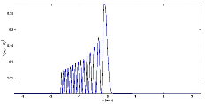
Figure 1: Field given by eq.(3), representing an Ideal Airy beam, with $x_{0}=100\,\mu$m and truncated, at $\zeta=0$, by a linear aperture of width $2X=3.3\,$mm. The quantities $a_{n}$ and coefficients $B_{n}$ are given by eqs.(5,9), with $m(s)=1$. We use $a_{R}=0.1$,  $L=50$, and $N=60$.

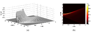
Figure 2: (a)Intensity of an Ideal Airy beam truncated by a finite aperture, as given by solution (4).(b) The same result depicted in orthogonal projection

In spite of the excellent results, we could get more accurate solutions by increasing the number of terms in the series (4), which expresses the resulting field, while keeping the same values for $L$ and $a_{R}$.

3.2 Analytic description of the truncated Airy-Exponential beam

Let us consider an Airy-Exponential beam truncated, at $\zeta=0$, by the same aperture of width $2X$; i.e., $\Psi(s,\zeta=0)=Ai(s)\,\exp(qs)\,(u(s+S)-u(s-S))$. Here we also chose $x_{0}=100\,\mu$m and $X=1.65\,$mm, with the value of $q$ set as $q=0.05$.

At $\zeta=0$ the field is approximately described by eq.(3), with $a_{n}$ and $B_{n}$ given by eqs.(5) and (9) respectively and with $m(s)=\exp(qs)$. Here we obtain quite good result by choosing, again, $L=50$,  $a_{R}=0.1$ and $N=60$.

Figure 3 shows the intensity of the field given by eq.(3) and we can see that it represents very well, at $z=0$, the truncated Airy-Exponential beam.

The resulting beam emanated by the aperture is given by solution (4), and its intensity is shown in Fig.4a. Figure 4b shows the orthogonal projection of this case.

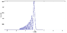
Figure 3: Field given by eq.(3), representing, at $z=0$, an Airy-Exponential beam, with $q=0.05$ and $x_{0}=100\,\mu$m, truncated by a linear aperture of width $2X=3.3\,$mm. The quantities $a_{n}$ and coefficients $B_{n}$ are given by eqs.(5,9) with $m(s)=\exp(qs)$. We use $a_{R}=0.1$,  $L=50$, and $N=60$.

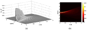
Figure 4: (a)Intensity of an Airy-Exponential beam truncated by a finite aperture, as given by solution (4).(b) The same result depicted in orthogonal projection

3.3 Analytic description of the truncated Airy-Gauss beam

Now, we wish to consider an Airy-Gauss beam truncated by a linear aperture of width $2X$; i.e., $\Psi(s,\zeta=0)=Ai(s)\,\exp(-qs^{2})\,(\theta(s+S)-\theta(s-S))$, with the spot size $x_{0}=100\,\mu$m, $X=1.65\,$mm and $q=5x_{0}^{2}/X^{2}=0.018$. This aperture possesses a size large enough to accommodate almost the entire power-flux of the Airy-Gauss beam.

At $\zeta=0$ this field is described by eq.(3), with $a_{n}$ and $B_{n}$ given by eqs.(5) and (9) respectively and with $m(s)=\exp(-qs^{2})$. In this case, an excellent result can be obtained by the choice $L=50$,  $a_{R}=0.1$ and $N=60$.

Figure 5 shows the intensity of the field given by eq.(3) and we can see that it represents, at $z=0$, the truncated Airy-Gauss beam with high fidelity

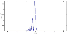
Figure 5: Field at $z=0$ given by eq.(3), representing an Airy-Gauss beam, with $q=0.018$ and $x_{0}=100\,\mu$m, truncated by a linear aperture of width $2X=3.3\,$mm. The quantities $a_{n}$ and coefficients $B_{n}$ are given by eqs.(5,9) with $m(s)=\exp(-qs^{2})$. We use $a_{R}=0.1$,  $L=50$, and $N=60$.

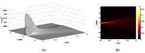
Figure 6: (a)Intensity of an Airy-Gauss beam truncated by a finite aperture, as given by solution (4).(b) The same result depicted in orthogonal projection

The beam emanated by the aperture is given by solution (4), and its intensity is shown in Fig.6a. This result corresponds to an Airy-Gauss beam truncated by a finite aperture. Figure 2b shows the orthogonal projection of this case.

4 Acknowledgments

The authors are grateful to Erasmo Recami, Hugo E. Hernández Figueroa, Jane M. Madureira Rached and Suzy Zamboni Rached for many stimulating contacts and discussions. The authors acknowledge partial support from FAPESP (under grant 11/51200-4); from CNPq (under grants 307962/2010-5 and 301079/2011-0).

5 Conclusion

In this paper we developed an analytic method capable to describe Airy-Type beams truncated by finite apertures.

This new approach is based on suitable superposition of Airy-Exponential beams and presents a simple analytic solution. The results agree with those already published in literature through the use of numerical methods. We demonstrated the method’s potentiality applying it to three different truncated Airy type beams: the Ideal Airy, the Airy-Gauss and the Airy-Exponential, but many others Airy-Type beams can easily be described with this analytic approach.

References

- [1] G. A. Siviloglou and D. N. Christodoulides, “Accelerating finite energy Airy beams,” Opt. Lett. 32, 979-981 (2007); and references therein.
- [2] M. I. Carvalho and M. Facão, “Propagation of Airy-related beams,” Opt. Express 18, 21938-21949 (2010)
- [3] G. A. Siviloglou, J. Broky, A. Dogariu, and D. N. Christodoulides, “Observation of accelerating Airy beams,” Phys. Rev. Lett. 99, 213901 (2007).
- [4] I. M. Besieris and A. M. Shaarawi,“A note on an accelerating finite energy Airy beam,” Opt. Lett. 32, 2447 (2007).