A nonequilibrium statistical model of spectrally truncated Burgers-Hopf dynamics

Abstract

Exact spectral truncations of the unforced, inviscid Burgers-Hopf equation are Hamiltonian systems with many degrees of freedom which exhibit intrinsic stochasticity and coherent scaling behavior. For this reason recent studies have employed these systems as prototypes to test stochastic mode reduction strategies. In the present paper the Burgers-Hopf dynamics truncated to $n$ Fourier modes is treated by a new statistical model reduction technique, and a closed system of evolution equations for the mean values of the $m$ lowest modes is derived for $m\ll n$. In the reduced model the $m$-mode macrostates are associated with trial probability densities on the phase space of the $n$-mode microstates, and a cost functional is introduced to quantify the lack of fit of paths of these densities to the Liouville equation. The best-fit macrodynamics is obtained by minimizing the cost functional over paths, and the equations governing the closure are then derived from Hamilton-Jacobi theory. The resulting reduced equations have a fractional diffusion and modified nonlinear interactions, and the explicit form of both are determined up to a single closure parameter. The accuracy and range of validity of this nonequilibrium closure is assessed by comparison against direct numerical simulations of statistical ensembles, and the predicted behavior is found to be well represented by the reduced equations.

1 Introduction

Throughout the applied mathematical sciences one meets complex nonlinear dynamical systems having large finite dimension, or infinite dimension, whose typical solutions exhibit chaotic or turbulent behavior. Often the same systems also reveal some organized structures that persist within the disordered fluctuations intrinsic to the dynamics. One is then faced with the challenge of describing such systems by appropriate model equations that synthesize the coherent behavior and the fluctuations, and that properly account for the interactions between them. A common approach is first to devise some low-dimensional governing equations for the coherent behavior and then to add some noise, or stochastic forcing, to capture the effect of the fluctuations. But if the original system is already described by an accepted set of governing equations that are deterministic, the question arises: in what sense is the stochastic model consistent with the given complex dynamics? To address this question of principle, it is necessary to derive the proposed stochastic model from the underlying deterministic dynamics by a systematic reduction technique [9, 14, 28, 24, 25].

This general problem of model reduction for complex dynamical systems, usually governed by nonlinear ODEs or PDEs, is conceptually identical to the generic problem of nonequilibrium statistical mechanics, which endeavors to connect macroscopic descriptions of systems consisting of a huge number of interacting particles or modes to the microscopic dynamics of their constituents [3, 15, 16, 22, 32, 33]. The standard approach in the field of statistical mechanics is to invoke projection operators that map the full phase space onto the span of some relevant, or resolved, dynamical variables, which define a macroscopic state. This method is used in the well-known Mori-Zwanzig formalism, which applies to an arbitrary set of resolved variables for a general Hamiltonian system [3, 33, 7, 8]. Typically these derivations make use of near-equilibrium assumptions to define tractable projection operators, and they lead to stochastic integro-differential equations having memory kernels and non-Markovian noise. While the fluctuation-dissipation theorem determines a key relation between the autocorrelation of the noise and the memory kernel, the evaluation of the kernel itself is determined by ensemble averages of the certain derived observables propagated under a complementary projection of the microdynamics. Consequently, it is normally imperative to make further approximations and simplifications, most notably taking a Markovian limit, to arrive at a useful and manageable model. As a result, systematic reductions of this kind are mostly confined to dynamical systems having special structures dictated by the methodology.

In recent work [31] one of the authors has proposed a new approach to statistical model reduction, which applies to any Hamiltonian dynamics and any suitable choice of resolved variables, and which leads directly from the given deterministic dynamics to closed reduced equations without recourse to intermediate stochastic approximations. This method of model reduction relies on a statistical optimization principle. First, a parametric statistical model is adopted consisting of trial probability densities on phase space associated with the mean values of the selected resolved variables. Then the reduced dynamics are determined by minimizing a cost functional over paths in the statistical parameter space. In this way a unique statistical closure is obtained once an appropriate cost functional is specified. The cost functional is designed to quantify the lack-of-fit of the path of trial densities to the underlying dynamics, and information-theoretic considerations suggest its form as a time-integrated, weighted, squared-norm on the residual of the trial densities with respect to the Liouville equation. A predicted, or estimated, evolution of the resolved variables therefore corresponds to a path in the statistical parameter space that best fits the underlying Hamiltonian dynamics in a sense quantified by the cost functional. All adjustable parameters in the closure appear as weights in the cost functional. These weights, which encode the influence of the unresolved fluctuations on the mean resolved evolution, are determined empirically.

The closed reduced equations that result from this dynamical optimization procedure have the desirable feature that they take the generic form of governing equations for nonequilibrium thermodynamics [10]. Namely, they are systems of first-order differential equations in the mean macrostate, and they contain a reversible term, which is a generalized Hamiltonian vector field, and an irreversible term, which is a gradient vector field [29]. Moreover, the structured derivation of these equations implies that the reversible and irreversible terms in the reduced equations correspond to terms in the cost function that quantify the resolved and unresolved components of the Liouville residual, respectively.

The purpose of the present paper is to illustrate and test this statistical reduction method by applying it to the Truncated Burgers-Hopf (TBH) equation. The untruncated version of this partial differential equation has long been a prototype for understanding fluid shock formation among other phenomena [21]. Its $n$-mode Fourier-Galerkin truncation, without forcing or viscosity, and for sufficiently large $n$, has been proposed as a good testbed for model reduction strategies, since it arises as the truncation of a familiar, one-dimensional nonlinear PDE and yet shares the statistical properties of many important complex dynamical systems [26, 27, 1, 24]. In particular, the TBH dynamics is chaotic and numerical simulations show it to be ergodic and mixing. The sharp truncation at wavenumber $n$ also leads to backscatter of energy from high to low wavenumbers, which produces coherent behavior in the low modes. It has a (noncanonical) Hamiltonian structure, and its equilibrium distribution is given by a Gibbs measure. In addition, it has the important statistical property that the decorrelation time of Fourier modes varies directly with their spatial scale [26], a property shared by important fluid dynamical systems such as those relevant to geophysical applications. The expository article [27] describes the properties of the model both analytically and numerically, and the paper [1] details the Hamiltonian structure, the invariants and the ensemble statistical behavior.

The abovementioned relationship between decorrelation time scale and wavenumber suggests a natural coarse-grained description in which the resolved modes are the lowest $m$ modes, for $m\ll n$. But, since every mode $k$ for $m+1\leq k\leq n$ is unresolved in this reduction, the separation of time scales between the resolved and unresolved modes is not wide. Consequently, the TBH dynamics poses a stringent test of any closure methodology, and the efficacy of a closure for the TBH system has implications for the the design of effective reduced descriptions of many high-dimensional, complex dynamics systems encountered in the physical sciences.

Our main result is an explicit $m$-mode reduced dynamics which has a structure similar to $m$-mode TBH dynamics itself, but with modified nonlinear interactions and strong, mode-dependent dissipation. Interestingly, the dissipation derived from the reduction procedure is not a standard diffusion, but rather a fractional diffusion. Furthermore, our statistical closure on $m$ resolved modes only depends on a single adjustable parameter, which scales the magnitude of the dissipation. By comparing the solutions of the reduced equations against ensemble averages of direct numerical simulations for $n=50$ and $m=5$, we show that the reduced equations of the statistical closure reproduce the true statistical evolution across the $m$-mode resolved spectrum, and for large as well as small initial conditions.

2 TBH dynamics and statistics

The unforced, inviscid Burgers-Hopf equation is the PDE

$$\frac{\partial u}{\partial t}+\frac{\partial}{\partial x}\left(\frac{1}{2}u^{2}\right)\,=\,0\,\;\;\;\;\;\;\;\;\;\;(\,x\in I\!\!R^{1}\,,t\geq 0\,)$$ (1)

for a scalar unknown $u=u(x,t)$. This equation has been extensively investigated as a simple prototype for the nonlinear behavior typical of the multi-dimensional equations of hydrodynamics, especially the formation of shock discontinuities and development of turbulence. For these considerations it is natural to consider the Burgers-Hopf equation with a finite viscosity and with forcing, which may be deterministic or stochastic. By contrast, the present work focusses exclusively on the free dynamics of spectral (or Galerkin) truncations the inviscid equation (1). These finite-dimensional dynamical system have been proposed as useful test systems for coarse-graining strategies and model reduction methodologies, which are intended to be applied to much more complex dynamic systems [26, 27, 1, 24].

We study the dynamics of the projection of $u$ onto the first $n$ modes of the Fourier series for $u$. For $2\pi$-periodic functions $u(x,t)$, $x\in[0,2\pi)$, the truncated series is defined by the projection operator,

$$(P_{n}u)(x,t)\,=\,\sum_{k=-n}^{n}z_{k}(t)\,e^{ikx}\,,\;\;\;\;\;\;\;\;\;\;z_{k}(t)=\frac{1}{2\pi}\int_{0}^{2\pi}u(x,t)\,e^{-ikx}\,dx\,.$$

The mean $z_{0}=\int_{0}^{2\pi}u(x,t)\,dx$ is a conserved quantity under (1), and so it is set to $0$ throughout. For a real solution $u(x,t)$, $z_{-k}=z^{*}_{k}$, for $k=1,\ldots,n$. [$z^{*}$ denotes complex conjugate of $z$.] The state space for the truncated dynamics with $n$ modes is therefore $\,l\!\!\!C^{n}$, and a generic state is a point $z=(z_{1},\ldots,z_{n})\in l\!\!\!C^{n}$. The governing dynamics for $u_{n}(x,t)=(P_{n}u)(x,t)$ is determined by the Galerkin truncation of (1), namely,

$$\frac{\partial u_{n}}{\partial t}+\frac{\partial}{\partial x}P_{n}\left(\frac{1}{2}u_{n}^{2}\right)\,=\,0\,.$$ (2)

In terms of the Fourier coefficients, $z=z(t)$, the Truncated Burger-Hopf (TBH) dynamics is accordingly the following system of $n$ quadratically nonlinear ODEs:

$$\frac{dz_{k}}{dt}+\frac{ik}{2}\sum_{k_{1}+k_{2}=k}z_{k_{1}}z_{k_{2}}\,=\,0\,,\;\;\;\;\;\;\;\;\;\;(k=1,\ldots,n).$$ (3)

where $k_{1},k_{2}$ run over $\{\pm 1,\ldots,\pm n\}$.

The dynamics (3) exactly conserves the following two quantities:

$$E\,=\,\frac{1}{4\pi}\int_{0}^{2\pi}u^{2}\,dx\,=\,\frac{1}{2}\sum_{k=-n}^{n}|z_{k}|^{2}\,,$$ (4)

$$H\,=\,\frac{1}{6\pi}\int_{0}^{2\pi}u^{3}\,dx\,=\,\frac{1}{6}\sum_{k_{1}+k_{2}+k_{3}=0}z_{k_{1}}z_{k_{2}}z_{k_{3}}\,.$$ (5)

The quadratic invariant, $E$, defines the total energy of the truncated system (3). Curiously, it is the cubic invariant, $H$, not the energy, $E$, that appears in the Hamiltonian form of the TBH dynamics (3); that is,

$$\frac{dz_{k}}{dt}\,=\,\sum_{k^{\prime}}J_{kk^{\prime}}\frac{\partial H}{\partial z_{k}^{*}}\,,\;\;\;\;\;\;\;\;\mbox{ for}\;\;\;\;J_{kk^{\prime}}=-ik\,\delta_{kk^{\prime}}\,,$$

where $\delta_{kk^{\prime}}=1$ if $k=k^{\prime}$, and $=0$ if $k\neq k^{\prime}$. These equations have the form of a noncanonical Hamiltonian system, or Poisson system, with cosymplectic matrix $J$ and Hamiltonian $H$, having $n$ complex degrees of freedom. Nonetheless, the invariant $H$ plays a much less prominent role in conditioning the dynamics than does the energy $E$, as has been documented by previous researchers [27, 1].

Except for $n=1,2$ the TBH dynamics is chaotic, and for $n>20$ numerical simulations indicate that it is ergodic and mixing. We therefore adopt a statistical mechanical perspective that focuses on the evolution of ensembles of solutions of (3), rather than individual solution trajectories. The Hamiltonian structure of (3) implies the Liouville property, namely, the invariance of phase volume, $dz=dx_{1}dy_{1}\ldots dx_{n}dy_{n}$, ($z_{k}=x_{k}+iy_{k}$) under the phase flow. Consequently, the propagation of probability by the TBH dynamics is represented in terms of a probability density $\rho(z,t)$ with respect to $dz$ that is transported according to the Liouville equation,

$$0\,=\,\frac{\partial\rho}{\partial t}+\sum_{k=1}^{n}\dot{x}_{k}\frac{\partial\rho}{\partial x_{k}}+\dot{y}_{k}\frac{\partial\rho}{\partial y_{k}}\,=\,\frac{\partial\rho}{\partial t}+\sum_{k=-n}^{n}\dot{z}_{k}\frac{\partial\rho}{\partial z_{k}}\,.$$ (6)

In principle, $\rho(z,t)$ is completely determined by (6), given an initial density $\rho(z,0)$, and hence the expectation of any observable $F$ on $l\!\!\!C^{n}$ at time $t>0$ is determined by

$$\langle F(t)\,|\,\rho\,\rangle=\int_{l\!\!\!C^{n}}F(z)\,\rho(z,t)\,dz\,.$$

[Throughout the paper $\langle F|\rho\rangle$ denotes expectation.] In practice, however, the exact density $\rho(z,t)$ evolves under the nonlinear, chaotic dynamics in an extremely complicated way, and numerical evaluation of the expectation of any observable with respect to $\rho(z,t)$ requires computing an ensemble of trajectories (3) starting from a sufficiently large sample of the initial density. This intrinsic feature of the dynamics, which is shared by many turbulent dynamical systems, is the fundamental reason for invoking model reduction procedures, which are devised to furnish sufficiently accurate approximations to those expectations without expensive sampling of the detailed dynamics.

Our reduction technique is based on using a convenient family of trial probability densities on the phase space to approximate the exact density evolving under (6). This family of nonequilibrium densities is constructed from a fixed reference equilibrium density, which we take to be the canonical ensemble,

$$\rho_{\beta}(z)=\frac{\exp(-\beta E(z))}{\int\exp(-\beta E(z))\,dz}\,=\,\prod_{k=1}^{n}\frac{\beta}{\pi}e^{-\beta|z_{k}|^{2}}\,,$$ (7)

with specified inverse temperature $\beta>0$. We choose the first $m$ components, $A(z)=(z_{1},\ldots,z_{m})$, of the microstate $z\in l\!\!\!C^{n}$ to be the resolved variables, or resolved modes, in the model. Experience with computed solutions of the TBH equation, as well as a heuristic scaling argument, informs this choice, because it is observed that the decorrelation time scales for the modes scale with $1/k$ [28, 23]. Accordingly, the lowest $m$ modes can be considered slow variables in the $n$-mode TBH dynamics. and the resolved vector $A$ constitutes a natural coarse-graining of the microstate $z\in l\!\!\!C^{n}$. We call the mean values $A$ the macrostate and denote it by $a=(a_{1},\ldots,a_{m})$. This coarse-grained description choice does not, however, ensure a wide separation of time scales between the resolved and unresolved variables, and consequently the TBH dynamics presents a rather challenging test for the model reduction technique.

The general properties of the non-equilibrium probability distributions of this system were examined numerically in [18] where it was noted that they are often quasi-normal. Motivated by this empirical observation, our statistical model employs the quasi-equilibrium (or quasi-canonical) densities

$$\tilde{\rho}(z;\lambda)\,=\,\exp\left(\sum_{k=-m}^{m}\lambda_{k}^{*}z_{k}-\frac{1}{2\beta}|\lambda_{k}|^{2}\right)\rho_{\beta}(z)\,,$$ (8)

This exponential family of densities (8) form a parametric statistical model, the parameter vector being $\lambda=(\lambda_{1},\ldots,\lambda_{m})\in l\!\!\!C^{m}$ [5, 19]. The convention, $\lambda_{-k}=\lambda_{k}^{*}$, for $k=1,\ldots,n$, and $\lambda_{0}=0$, applies to the parameters. Since $\rho_{\beta}$ is a Gaussian density, each density $\tilde{\rho}(\lambda)$ is also Gaussian; with respect to $\tilde{\rho}(\lambda)$ the means and variances of the resolved variables are

$$a_{k}=\langle\,z_{k}\,|\,\tilde{\rho}(\lambda)\,\rangle\,=\,\frac{1}{\beta}\,\lambda_{k}\,,\;\;\;\;\;\;\;\;\langle\,(z_{k}-a_{k})(z_{k^{\prime}}-a_{k^{\prime}})^{*}\,|\,\tilde{\rho}(\lambda)\,\rangle\,=\,\frac{1}{\beta}\,\delta_{kk^{\prime}}\,,$$ (9)

for $k,k^{\prime}=\pm 1,\ldots,\pm m$. A highly desirable feature of the statistical model (8) is that all the modes $z_{k}$ are independent and the correspondence between the mean resolved variables $a_{k}$ and the statistical parameters $\lambda_{k}$ is linear and decoupled.

Other possible choices of statistical model are conceivable. For instance, the invariance of both $E$ and $H$ suggests using the more general equilibrium density

$$\rho_{\beta,\alpha,\eta}(z)\,=\,Q(\beta,\alpha,\eta)^{-1}\exp(\,-\beta E(z)-\eta E(z)^{2}-\alpha H(z)\,)$$

with $\eta>0$; $Q(\beta,\alpha,\eta)$ is the normalizing factor. This density is a so-called Gaussian ensemble with respect to $E$, as it includes the quadratic term $E^{2}$ in the exponential, which is necessary to make the density normalizable given the presence of the cubic invariant $H$. But, using $\rho_{\beta,\alpha,\eta}$ as the reference density for the statistical model $\tilde{\rho}(\lambda)$ leads to non-Gaussian trial densities, and hence an intractable subsequent analysis. Fortunately, simulations of ensembles of solutions of the TBH dynamics have shown that the distribution of the modes $z_{k}$ is very nearly Gaussian, and that $H$ has only a slight effect on the statistical behavior, provided that the mean value $\langle H\rangle$ is close enough to the relaxed value $\langle H\,|\,\rho_{\beta}\rangle=0\;$ [28, 23, 1]. Accordingly, our statistical model and closure procedure are built from the reference density (7) that does not include $H$. In this formulation we expect to approximate a statistical evolution in which the mean value of $H$ is near its relaxed value, but not an evolution from an initial statistical state with a large mean value of $H$.

Neither $\langle E|\tilde{\rho}(\lambda)\rangle$ nor $\langle H|\tilde{\rho}(\lambda)\rangle$ is exactly conserved along an arbitrary admissible path $\lambda=\lambda(t)$ in the statistical parameter space. It is possible to alter the formulation of the statistical model to ensure that both of these invariants are respected, but with the inevitable consequence that the trial densities are non-Gaussian [31]. Our main justification for allowing some variation in these dynamical invariants is, therefore, expediency, combined with the fact that for $n\gg m$ the relative variations in the means of $E$ and $H$ are small.

3 Formulating the optimization principle

Our $m$-mode closure of the $n$-mode TBH dynamics is derived from an optimization principle over paths, $\lambda(t)$, in the parameter space, $l\!\!\!C^{m}$, of the statistical model (8). A predicted, or estimated, evolution of the macrostate $a=a(t)$, with $a_{k}(t)=\langle\,z_{k}\,|\,\tilde{\rho}(\lambda(t))\,\rangle$ for $k=1,\ldots,m$, corresponds to a path $\lambda(t)$ that is optimally compatible with the underlying TBH dynamics, in the sense that $\lambda(t)$ minimizes a certain lack-of-fit cost functional over all admissible paths. This lack-of-fit is a metric on the Liouville residual, a fundamental statistic in our approach that we define to be

$$R\,=\,\left(\,\frac{\partial}{\partial t}+\sum_{k=-n}^{n}\frac{dz_{k}}{dt}\frac{\partial}{\partial z_{k}}\,\right)\log\tilde{\rho}(\cdot\,;\lambda(t))\,=\,\sum_{k=-m}^{m}\dot{\lambda}_{k}^{*}(z_{k}-a_{k})+\lambda_{k}^{*}\frac{dz_{k}}{dt}\,.$$ (10)

Here $dz_{k}/dt$ is given by the governing TBH dynamics (3), and $\dot{\lambda}_{k}=d\lambda_{k}/dt$. If $\tilde{\rho}(\cdot\,;\lambda(t))$ is replaced by an exact solution $\rho(\cdot\,,t)$ of (6) in (10), then $R=0$ identically on the phase space $l\!\!\!C^{n}$. In [31] it is shown that the statistic $R=R(z;\lambda,\dot{\lambda})$ may be interpreted as the local rate of information loss at the sample point $z$ due to reduction via the statistical model (8). The significance of $R$ is also revealed by the family of identities

$$\frac{d}{dt}\langle\,F\,|\,\tilde{\rho}(\lambda(t))\,\rangle\,-\,\langle\,\dot{F}\,|\,\tilde{\rho}(\lambda(t))\,\rangle\,=\,\langle\,FR\,|\,\tilde{\rho}(\lambda(t))\,\rangle\,,$$

which hold for every observable $F$ on $l\!\!\!C^{n}$, with $\partial F/\partial t=0$; here, $\dot{F}=\{F,H\}$ denotes the Poisson bracket of $F$ with $H$, so that $dF(z(t))/dt=\dot{F}(z(t))$ on solutions $z=z(t)$ of (3). Since the mean of $R$ with respect to $\tilde{\rho}(\lambda)$ is zero, $\langle R|\tilde{\rho}\rangle=0$, the covariance between an observable $F$ and the Liouville residual $R$ quantifies the deficiency of the path of trial densities $\tilde{\rho}(\lambda(t))$ to propagate the expectation of $F$. This family of identities over test observables furnishes a natural linear structure for defining the lack-of-fit of any admissible path $\lambda(t)$ to the underlying dynamics, and motivates the use of a weighted $L^{2}(l\!\!\!C^{n},\tilde{\rho}(\lambda))$ squared norm as the lack-of-fit cost function.

The weights in the lack-of-fit cost function relate to the resolved and unresolved subspaces of $L^{2}(l\!\!\!C^{n},\tilde{\rho}(\lambda))$. The mean-centered resolved variables

$$U_{k}=z_{k}-a_{k}\,=\,\frac{\partial}{\partial\lambda_{k}}\log\tilde{\rho}(\cdot\,;\lambda)\,\;\;\;\;\;\;\;\;\;\;(\,k=1,\ldots,m\,)\,,$$ (11)

span the resolved subspace, and, by (9), they are uncorrelated Gaussian variables, $\langle U_{k}U_{k^{\prime}}^{*}\rangle=\beta^{-1}\delta_{kk^{\prime}}$, for all $\lambda\in l\!\!\!C^{n}$. The orthogonal projection of $L^{2}(l\!\!\!C^{n},\tilde{\rho})$ onto the resolved subspace is

$$P_{A}F\,=\,\beta\sum_{k=-m}^{m}\langle\,FU_{k}^{*}\,|\,\tilde{\rho}\,\rangle\,U_{k}\,,$$ (12)

and the complementary projection onto the unresolved subspace (the orthogonal complement of the resolved subspace) is $Q_{A}=I-P_{A}$. The projections of the Liouville residual $R=R(\lambda,\dot{\lambda})$ onto its resolved and unresolved components are calculated to be

$$P_{A}R\,=\,\beta\sum_{k=-m}^{m}\left[\,\dot{a}_{k}+\frac{ik}{2}\sum_{k_{1}+k_{2}=k}a_{k_{1}}a_{k_{2}}\,\right]^{*}U_{k}$$ (13)

$$Q_{A}R\,=\,\frac{-i\beta}{2}\sum_{k=-m}^{m}ka_{k}^{*}\sum_{k_{1}+k_{2}=k}U_{k_{1}}U_{k_{2}}\,=\,\frac{i\beta}{2}\sum_{k_{1}+k_{2}+k_{3}=0}k_{3}a_{k_{3}}U_{k_{1}}U_{k_{2}}\,.$$ (14)

Here, $\dot{a}_{k}=da_{k}/dt=\dot{\lambda}_{k}/\beta$. Since $a_{k}=0$ for $|k|>m$, the wavenumber indices $k_{1},k_{2}$ in (13) run over $\{\pm 1,\ldots,\pm m\}$, unlike the nonlinear term in the TBH dynamics, in which all modes in $\{\pm 1,\ldots,\pm n\}$ interact with the resolved modes. By contrast, $k_{1},k_{2}$ in (14) run over $\{\pm 1,\ldots,\pm n\}$, and the definition of $U_{k}$ is extended for $|k|>m$ to be simply $U_{k}=z_{k}$.

The identities (13) and (14) make use of the following identities for the Gaussian scores variables:

$$\langle\,U_{k_{1}}U_{k_{2}}U_{k_{3}}\,|\,\tilde{\rho}\,\rangle = 0\,,$$ (15)

$$\langle\,U_{k_{1}}U_{k_{2}}U_{k^{\prime}_{1}}^{*}U_{k^{\prime}_{2}}^{*}\,|\,\tilde{\rho}\,\rangle = \frac{1}{\beta^{2}}[\,\delta_{k_{1}k^{\prime}_{1}}\delta_{k_{2}k^{\prime}_{2}}+\delta_{k_{1}k^{\prime}_{2}}\delta_{k_{2}k^{\prime}_{1}}\,]\,.$$

The calculations (13) and (14) are summarized as follows. In light of (10),

$$P_{A}R\,=\,\sum_{k=-m}^{m}\dot{\lambda}_{k}^{*}U_{k}+\lambda_{k}^{*}\beta\sum_{k^{\prime}=-m}^{m}\langle\,\frac{dz_{k}}{dt}\,U_{k^{\prime}}^{*}\,\rangle\,U_{k^{\prime}}\,.$$

Substituting (3) and using $\beta\langle\,z_{k_{1}}z_{k_{2}}U_{k^{\prime}}^{*}\,\rangle=a_{k_{1}}\delta_{k_{2}k^{\prime}}+a_{k_{2}}\delta_{k_{1}k^{\prime}}\,$, which is implied by (15), results in

$$P_{A}R = \sum_{k=-m}^{m}\dot{\lambda}_{k}^{*}U_{k}+\lambda_{k}^{*}\,ik\sum_{k^{\prime}=-m}^{m}a_{k-k^{\prime}}U_{k^{\prime}}$$

$$= \sum_{k=-m}^{m}\left\{\dot{\lambda}_{k}^{*}-i\sum_{k^{\prime}=-m}^{m}k^{\prime}\lambda_{k^{\prime}}^{*}a_{k-k^{\prime}}^{*}\right\}U_{k}$$

$$= \sum_{k=-m}^{m}\left\{\dot{\lambda}_{k}^{*}+i\sum_{k_{1}+k_{2}=k}k_{1}\lambda_{k_{1}}a_{k_{2}}\right\}^{*}U_{k}\,.$$

Putting $\lambda_{k}=\beta a_{k}$ and using the symmetry between $k_{1}$ and $k_{2}$ then produces the desired identity (13). In a similar manner,

$$Q_{A}R = R\,-\,P_{A}R$$

$$= \sum_{k=-m}^{m}\lambda_{k}^{*}\left[\frac{dz_{k}}{dt}+\,ik\sum_{k^{\prime}=-m}^{m}a_{k-k^{\prime}}\right]U_{k^{\prime}}$$

$$= -\frac{i}{2}\sum_{k=-m}^{m}k\lambda_{k}^{*}\sum_{k_{1}+k_{2}=k}z_{k_{1}}z_{k_{2}}-a_{k_{1}}U_{k_{2}}-a_{k_{2}}U_{k_{1}}$$

$$= -\frac{i}{2}\sum_{k=-m}^{m}k\lambda_{k}^{*}\sum_{k_{1}+k_{2}=k}U_{k_{1}}U_{k_{2}}-a_{k_{1}}a_{k_{2}}\,,$$

using the symmetry between $k_{1}$ and $k_{2}$ in the third equality. The constant term in the last expression vanishes, because

$$\sum_{k=-m}^{m}k\lambda_{k}^{*}\sum_{k_{1}+k_{2}=k}a_{k_{1}}a_{k_{2}}\,=\,-\beta\sum_{k_{1}+k_{2}+k_{3}=0}k_{3}a_{k_{1}}a_{k_{2}}a_{k_{3}}\,=\,0\,,$$

and hence the desired identities (14) follow.

The cost function for our optimization principle is declared to be

$${\mathcal{L}}(\lambda,\dot{\lambda})\,=\,\frac{1}{2}\langle\,[P_{A}R(\lambda,\dot{\lambda})]^{2}\,|\,\tilde{\rho}(\lambda)\,\rangle+\frac{1}{2}\langle\,[WQ_{A}R(\lambda,\dot{\lambda})]^{2}\,|\,\tilde{\rho}(\lambda)\,\rangle\,,$$ (16)

in which $W$ is a linear operator on $L^{2}(l\!\!\!C^{n},\tilde{\rho})$ satisfying $WP_{A}=P_{A}W$. We refer to $W$ as the weight operator, because it weights the contributions of the unresolved component, $Q_{A}R$, of the Liouville residual $R$ relative to the (unit weighted) resolved component, $P_{A}R$. The requirement that $W$ commutes with the projection $P_{A}$ implies that $W$ also commutes with $Q_{A}$ and hence that $W$ takes the unresolved subspace into itself. The inclusion of $W$ in the cost function (16) gives our best-fit closure the character of a weighted least-squares approximation over paths $\lambda(t)$.

With this cost function in hand, we are now able to formulate the optimization principle that defines our statistical closure. In this section we present the stationary version of the principle, which is simpler to describe and motivate. A nonstationary version, which is needed when comparing the predictions of the closure with direct numerical simulations, is given in Section 6.

The best-fit closure scheme is based on the dynamical minimization problem

$$v(\lambda^{0})\,=\,\min_{\lambda(t_{0})=\lambda^{0}}\;\int_{t_{0}}^{+\infty}{\mathcal{L}}(\lambda,\dot{\lambda})\,dt\,,$$ (17)

in which the admissible paths $\lambda(t),\;t_{0}\leq t<+\infty\,$, in the configuration space of the statistical model are constrained to start at $\lambda^{0}\in l\!\!\!C^{n}$ at time $t_{0}$. In optimization and control theory, $v(\lambda^{0})$ is called the value function for the minimization problem (17) [4, 11, 12]. Since ${\mathcal{L}}(\lambda,\dot{\lambda})$ is independent of $t$, and the integration extends to infinity in time, $v(\lambda)$ is time-independent, and the initial time $t_{0}$ may be shifted to $0$ in (17).

By analogy to analytical mechanics, one may regard (17) as a principle of least action for the “Lagrangian” ${\mathcal{L}}(\lambda,\dot{\lambda})$ and interpret the first member in (23) as its “kinetic” term and the second member as its “potential” term [2, 13, 20]. The kinetic term is a positive-definite quadratic form in the generalized velocities $\dot{\lambda}$, and it is entirely determined by the structure of the resolved variables and trial densities. By contrast, the potential term embodies the influence of the unresolved variables on the resolved variables and involves the weight operator $W$, which contains all the adjustable closure parameters.

Each extremal path $\hat{\lambda}(t)$, $t_{0}\leq t<+\infty$, for (17) corresponds to an evolving trial density $\tilde{\rho}(\,\cdot\,;\hat{\lambda}(t))$ that is best-fit to the Liouville equation in the sense that the time-integral of the lack-of-fit cost function is minimized. Finiteness of the value function implies that $\lambda(t)\rightarrow 0$ as $t\rightarrow+\infty$, meaning that the best-fit path connects the given initial state $\lambda^{0}$ to equilibrium $\lambda^{eq}=0$. Hence, these extremal paths model the relaxation of the mean resolved vector $\hat{a}(t)=\langle A\,|\tilde{\rho}(\hat{\lambda}(t))\rangle$, from a given initial state $a^{0}=\langle A\,|\tilde{\rho}(\lambda^{0})\rangle$.

It is important to emphasize that the weight operator $W$ is an independent ingredient in our closure strategy and that $W$ includes all the empirical parameters in the best-fit closure. It is unavoidable that some empirical ingredient should enter into the definition of such a closure, because the defining optimization principle does not refer to the autocorrelations of the unresolved modes under the full dynamics, or the projected dynamics orthogonal to the resolved subspace. As is well-known in nonequilibrium statistical mechanics, the transport properties of the complex system, as well as the memory kernels in its projected dynamics, are expressible in terms of such autocorrelations [3, 6, 32, 33]. In this light our closure strategy of adopting a time-integrated, weighted, least-squares approximation is a practical expedient to avoid the expensive computation of such autocorrelations, which require the propagation of ensembles of solutions of the fully resolved dynamics. Our approach instead quantifies the influence of the unresolved modes on the resolved modes by an appropriately chosen weight operator $W$ which depends on some adjustable parameters that must be tuned empirically.

In this general formulation of the optimization principle, the weight operator $W$ is not restricted to any particular form. Moreover, the closed reduced equations satisfied by its extremals have a generic thermodynamic format and associated properties for any admissible choice of $W$ [31]. In any concrete implementation of the best-fit approach, however, it is essential to discern a convenient form for $W$ from the structure of the underlying dynamics, the resolved variables and the unresolved Liouville residual. It is also desirable to choose a weight operator that contains as few adjustable parameters as possible, given the required level of fidelity of the closure approximation to the true statistical dynamics. In the Burgers-Hopf dynamics the quadratic nonlinearity, typical of hydrodynamics, affords a particularly simple and efficacious choice of $W$, as is described in the next section.

4 Deriving the closed reduced dynamics

First, let us consider the implications of the trivial choice for the weight operator in (16), namely, $W=0$. In that situation the solution of the minimization problem (17) is complete determined by setting $P_{A}R=0$ at each instant of time. The resolved vector, $a=(a_{1}(t),\ldots,a_{m}(t))=(\langle z_{1}|\tilde{\rho}\rangle,\ldots,\langle z_{m}|\tilde{\rho}\rangle)$, then satisfies

$$\frac{da_{k}}{dt}+\frac{ik}{2}\sum_{k_{1}+k_{2}=k}a_{k_{1}}a_{k_{2}}\,=0\;\;\;\;\;\;\;\;\;\;\;\;\;\;(k=1,\ldots,m)\,,$$

meaning that the reduced dynamics coincides with the spectral truncation to $m$ modes of the Burgers-Hopf equation. Not only are the $m$-mode truncations of $E$ and $H$ invariant under this dynamics, but the entropy,

$$s\,=\,-\langle\,\log\tilde{\rho}\,|\,\tilde{\rho}\,\rangle\,=\,-\frac{\beta}{2}\sum_{k=-m}^{m}|a_{k}|^{2}\,,$$ (18)

is also invariant; indeed, the entropy production is

$$\frac{ds}{dt}\,=\,-\,\beta\sum_{k=-m}^{m}a_{k}^{*}\,\frac{da_{k}}{dt}\;=\;\frac{i\beta}{2}\sum_{k_{1}+k_{2}+k_{3}=0}k_{3}a_{k_{1}}a_{k_{2}}a_{k_{3}}\,=0\,.$$

This naive closure is therefore adiabatic, in that it suppresses interactions between the resolved modes and the unresolved modes, those interactions being the source of entropy production and dissipation in a proper reduced dynamics.

Now, we seek an effective choice of $W$ that appropriately quantifies the cost of the unresolved component of the Liouville residual as well as the resolved component. An examination of (14) reveals that unresolved residual, $Q_{A}R$, is a linear combination of the products $U_{k_{1}}U_{k_{2}}$ over $k_{1},k_{2}=\pm 1,\ldots,\pm n$. This structure is a consequence of the quadratic nonlinearity of the TBH dynamics. Since these products form an orthogonal basis for the unresolved subspace, it is natural and convenient to construct the desired weight operator in terms of them. Accordingly, we take $W$ to be diagonal with respect to this basis and we set

$$W(U_{k_{1}}U_{k_{2}})\,=\,\epsilon_{k_{1},k_{2}}\,(U_{k_{1}}U_{k_{2}})\,,$$ (19)

for some sequence of constants $\epsilon_{k_{1},k_{2}}\geq 0$, symmetric with respect to interchanging $k_{1}$ with $k_{2}$. The “potential” term in the cost function (16) is then

$$\frac{1}{2}\langle\,[WQ_{A}R(\lambda,\dot{\lambda})]^{2}\,|\,\tilde{\rho}(\lambda)\,\rangle = \frac{1}{4}\sum_{k=-m}^{m}k^{2}|a_{k}|^{2}\cdot\sum_{k_{1}+k_{2}=k}\epsilon_{k_{1},k_{2}}^{2}\langle\,U_{k_{1}}U_{k_{2}}U_{k_{1}}^{*}U_{k_{2}}^{*}\,\rangle$$ (20)

$$= \frac{1}{2\beta^{2}}\sum_{k=-m}^{m}\gamma_{k}\,k^{2}|a_{k}|^{2}\,,$$

with

$$\gamma_{k}\,=\,\frac{1}{2}\sum_{k_{1}+k_{2}=k}\epsilon_{k_{1},k_{2}}^{2}\;\;\;\;\;\;\;\;\;\;\;\;(\,k=1,\ldots,m\,)\,.$$ (21)

The sums in (20) and (21) extend over $1\leq|k_{1}|,|k_{2}|\leq n$. The calculation in (20) uses the fourth moments in (15). We thus arrive at the explicit expression for the cost function,

$${\mathcal{L}}(\lambda,\dot{\lambda})\,=\,\frac{1}{2}\sum_{k=-m}^{m}\frac{1}{\beta}\left|\,\dot{\lambda}_{k}+\frac{ik}{2\beta}\sum_{k_{1}+k_{2}=k}\lambda_{k_{1}}\lambda_{k_{2}}\,\right|^{2}\,+\,\frac{\gamma_{k}\,k^{2}}{\beta^{2}}\,|\lambda_{k}|^{2}\,,$$ (22)

which follows from (16) by (13) and (20), together with the simple relations given in (9).

We notice that the weights $\epsilon_{k_{1},k_{2}}$ defining $W$ enter the cost function ${\mathcal{L}}$ only though the combinations $\gamma_{1},\ldots,\gamma_{m}$ in (21). While it is possible to retain these $m$ adjustable parameters in the closure, their form as sums over the weights $\epsilon_{k_{1},k_{2}}$ suggests a further simplification. Namely, for $1\leq k\leq m\ll n$, the $\gamma_{k}$ in (21) are approximately independent of $k$, whenever the weight sequence $\epsilon_{k_{1},k_{2}}$ is chosen to be bounded and slowly varying over the range $1\leq|k_{1}|,|k_{2}|\leq n$. On this basis it is reasonable to set $\gamma_{k}=\gamma>0$, for $k=1,\ldots,m$, and to adopt a cost function with a single adjustable parameter, $\gamma$. We confine ourselves to this simplified formulation throughout the present paper. This choice of cost function is also justified a posteriori by our subsequent analysis, which shows that the scaling of the modal dissipation rates with $|k|$ implied by a constant $\gamma$ agrees with the direct numerical simulations presented in Sections 7 and 8 as well as the formal dimensional argument summarized in Section 5. Indeed, we find that the TBH dynamics is an example of a complex system in which the effect of unresolved modal fluctuations on the resolved modes is efficiently and accurately modeled by a lack-of-fit cost function having a single, empirically-tuned, closure parameter.

The equations satisfied by the extremal paths for (17) are found by the techniques of the calculus of variations [4, 12, 11, 13, 30]. In particular, Hamilton-Jacobi theory furnishes the the closed reduced equations for the statistical model in terms of the value function $v(\lambda)$. To this end we write the cost-function (22) in the more compact form,

$${\mathcal{L}}(\lambda,\dot{\lambda})\,=\,\sum_{k=1}^{m}\frac{1}{\beta}\left|\,\dot{\lambda}_{k}-\beta f_{k}(\lambda)\,\right|^{2}\,+\,\frac{\gamma\,k^{2}}{\beta^{2}}\,|\lambda_{k}|^{2}\,,$$ (23)

introducing the shorthand notation

$$f_{k}(\lambda)\,=\,-\frac{ik}{2\beta^{2}}\sum_{k_{1}+k_{2}=k}\lambda_{k_{1}}\lambda_{k_{2}}\,.$$ (24)

and recalling that $\lambda_{-k}=\lambda_{k}^{*}$. We form the Hamiltonian ${\mathcal{H}}(\lambda,\mu)$ conjugate to the Lagrangian ${\mathcal{L}}(\lambda,\dot{\lambda})$ by taking the Legendre transform of ${\mathcal{L}}$:

$$\mu_{k} = \frac{\partial{\mathcal{L}}}{\partial\dot{\lambda}_{k}^{*}}\,=\,\frac{1}{\beta}\dot{\lambda}_{k}-f_{k}(\lambda)\,,$$ (25)

$${\mathcal{H}}(\lambda,\mu) = \sum_{k=1}^{m}\mu_{k}^{*}\dot{\lambda}_{k}+\dot{\lambda}_{k}^{*}\mu_{k}-{\mathcal{L}}(\lambda,\dot{\lambda})$$

$$= \sum_{k=1}^{m}\beta|\mu|^{2}+\beta[\,\mu_{k}^{*}f_{k}(\lambda)+f_{k}(\lambda)^{*}\mu_{k}\,]-\frac{\gamma}{\beta^{2}}k^{2}|\lambda_{k}|^{2}\,.$$

[That these complex expressions are appropriate complexifications of the real Legendre transform is shown in the Appendix.]

The value function, $v(\lambda)$, in (17), which is analogous to an action integral or Hamilton principal function, satisfies the stationary Hamilton-Jacobi equation:

$${\mathcal{H}}\left(\lambda,\,-\frac{\partial v}{\partial\lambda^{*}}\right)\,=\,0\,,$$ (26)

According to Hamilton-Jacobi theory, the conjugate variable $\mu=\hat{\mu}(t)$ along an extremal path $\lambda=\hat{\lambda}(t)$ is given by the relation

$$\hat{\mu}\,=\,-\frac{\partial v}{\partial\lambda^{*}}(\hat{\lambda})\,.$$ (27)

This key relation closes the reduced dynamics along the extremal path, since together with (25) it yields the system of first-order ODEs

$$\frac{d\hat{a}_{k}}{dt}\,=\,f_{k}(\hat{\lambda})\,-\,\frac{\partial v}{\partial\lambda_{k}^{*}}(\hat{\lambda})\,,\;\;\;\;\;\;\;\;\;\;\;\;(\,k=1,\ldots,m\,)$$ (28)

recalling that $\hat{a}_{k}=\hat{\lambda}_{k}/\beta$. When expressed entirely in terms of the mean resolved variables, the closed reduced equations are

$$\frac{d\hat{a}_{k}}{dt}+\frac{ik}{2}\sum_{k_{1}+k_{2}=k}\hat{a}_{k_{1}}\hat{a}_{k_{2}}\,=\,-\frac{\partial v}{\partial\lambda_{k}^{*}}(\beta\hat{a})\,.$$ (29)

The left-hand side of this system of equations is recognizable as the $m$-mode TBH dynamics. The adiabatic closure mentioned earlier in this section is obtained by setting $v=0$ identically in (29). The presence of the gradient vector field of $v$ on the right hand side provides the dissipation, or irreversibility, of the closed reduced dynamics. Indeed, the relation (27) has the interpretation that the conjugate vector $\mu$ to the statistical state vector $\lambda$ represents the irreversible part of the flux of the mean resolved vector $a$.

The best-fit closure (28,29) is completed once the value function (17) is determined explicitly, at least to some suitable approximation. This calculation is the content of the next section.

5 Approximating the value function

Before presenting the nonlinear analysis needed to approximate the value function, we exhibit the first-order, linear approximation in the near-equilibrium regime, which can be obtained by elementary methods. We consider the relaxation of a small initial disturbance from equilibrium, and so we retain only the quadratic terms in the cost function (23), which becomes

$${\mathcal{L}}(\lambda,\dot{\lambda})\,=\,\sum_{k=1}^{m}\frac{1}{\beta}|\,\dot{\lambda}_{k}|^{2}\,+\,\frac{\gamma\,k^{2}}{\beta^{2}}\,|\lambda_{k}|^{2}\,.$$

Each extremal, $\hat{\lambda}(t)$, solves the Euler-Lagrange equations for (17) for this integrand,

$$-\frac{d^{2}\hat{\lambda}_{k}}{dt^{2}}+\frac{\gamma k^{2}}{\beta}\hat{\lambda}_{k}\,=\,0\,.$$

Since the admissible paths connect the initial state to equilibrium as $t\rightarrow+\infty$, the relevant extremals are the exponentially decaying solutions,

$$\hat{\lambda}_{k}(t)=\lambda_{k}(0)\exp\left(-\sqrt{\frac{\gamma}{\beta}}\,|k|t\right).$$

The near-equilibrium closed reduced equations satisfied by these extremals are

$$\frac{d\hat{a}_{k}}{dt}\,=\,-\sqrt{\frac{\gamma}{\beta}}\,|k|\,\hat{a}_{k}\,,$$ (30)

and the value function evaluated on these extremals is

$$v(\lambda)\,=\,\sqrt{\frac{\gamma}{\beta^{3}}}\,\sum_{k=1}^{m}k\,|\lambda_{k}|^{2}\,.$$

The elementary result (30) is consistent with (28), since $f=0$ in this approximation. Moreover, the same result is anticipated by a heuristic scaling argument in [26, 27]. Phenomenological reasoning about the transfer of energy in the turbulent TBH system suggests forming an eddy turnover time, $T_{k}$, for the $k$-th mode from the wavenumber, $k$, and the energy per mode in statistical equilibrium, $1/\beta$. The only dimensionally consistent time scale is $T_{k}\sim\sqrt{\beta}/k$. It is well confirmed by direct numerical simulations of the TBH dynamics in [26, 27] that the equilibrium autocorrelations of the modes, $z_{k}$, exhibit the $k$-dependent decay rate proportional to $T_{k}^{-1}$ across the spectrum, thus validating this scaling argument. To relate our basic prediction (30) to this scaling theory and its validating numerical simulations we rely on linear response theory, which holds for relaxation near equilibrium and connects the nonequilibrium mean value of the resolved variables $A_{k}$ to their equilibrium autocorrelations [6, 15, 33]. Precisely, the ensemble mean of $A_{k}(t)$, the resolved variable propagated under the phase flow for time $t$, with respect to an initial quasi-equilibrium density $\tilde{\rho}(\lambda^{0})$ for small $|\lambda^{0}|$ is calculated up to linear-response approximations to be

$$\langle A_{k}(t)\,|\,\tilde{\rho}(\lambda^{0})\rangle\,\approx\langle A_{k}(t)\,[1+\sum_{k^{\prime}=-m}^{m}(\lambda_{k^{\prime}}^{0})^{*}A_{k^{\prime}}]\rangle_{eq}=\sum_{k^{\prime}=-m}^{m}\langle A_{k}(t)A_{k^{\prime}}^{*}\rangle_{eq}\,\lambda_{k^{\prime}}^{0}\,.$$

Thus the time scale for decay of $\langle A_{k}(t)\,|\,\tilde{\rho}(\lambda^{0})\rangle$ is dictated by the time scalings of the decaying autocorrelations $\langle A_{k}(t)A_{k^{\prime}}^{*}\rangle_{eq}$. In light of the robust scaling behavior of the autocorrelations, the decay rates in (30) are necessarily proportional to $|k|/\sqrt{\beta}$. This correspondence also validates the choice of the weight operator in the cost function and the further simplification to a single closure parameter $\gamma$, independent of $k$.

We now turn to the nonlinear problem of determining an approximation to $v(\lambda)$ that is valid for larger amplitudes $|\lambda|$. We seek an solution that is accurate up to cubic terms in $\lambda$, so that the resulting gradient term in (29) contributes quadratically-accurate nonlinear terms. Accordingly, we submit a third-order Taylor expansion for $v$ to the Hamilton-Jacobi equation (26):

$$v(\lambda)\,=\,\sum_{k=1}^{m}M_{k}|\lambda_{k}|^{2}\,+\,\sum_{k_{1},k_{2},k_{3}}N_{k_{1}k_{2}k_{3}}\lambda_{k_{1}}\lambda_{k_{2}}\lambda_{k_{2}}\,+\ldots\,.$$ (31)

The constant and first-order terms in (31) vanish, since $v(0)=0=\partial v/\partial\lambda(0)$. The quadratic terms in the expansion (31) already have the special form anticipated by the foregoing linear analysis, with real and positive coefficients $M_{k}$. The indices $k_{1},k_{2},k_{3}$ for the cubic terms run over $\{\pm 1,\ldots,\pm m\}$, and the complex coefficients $N_{k_{1}k_{2}k_{3}}$ are assumed to be symmetric under permutation of $k_{1},k_{2},k_{3}$ and to satisfy $N_{-k_{1},-k_{2},-k_{3}}=N_{k_{1}k_{2}k_{3}}^{*}$, since $v(\lambda)$ is a real-valued function. These requirements supplemented the convention that $\lambda_{-k}=\lambda_{k}^{*}$ and $\mu_{-k}=\mu_{k}^{*}$. The reader is referred to the Appendix for a summary of the appropriate form of Taylor’s theorem for functions of several complex variables.

The Hamiltonian in (26), when written in full using (24), is

$${\mathcal{H}}(\lambda,\mu)\,=\,\sum_{k=1}^{m}\beta|\mu_{k}|^{2}-\frac{\gamma}{\beta^{2}}k^{2}|\lambda_{k}|^{2}\;+\,\frac{i}{2\beta}\sum_{k_{1}+k_{2}+k_{3}=0}k_{3}\lambda_{k_{1}}\lambda_{k_{2}}\mu_{k_{3}}\,.$$ (32)

The leading term in (26) is evaluated as follows:

$$\sum_{k=1}^{m}\left|\frac{\partial v}{\partial\lambda_{k}^{*}}\right|^{2} = \sum_{k=1}^{m}\frac{\partial v}{\partial\lambda_{k}}\frac{\partial v}{\partial\lambda_{-k}}$$

$$= \sum_{k=1}^{m}M_{k}^{2}|\lambda_{k}|^{2}\,+\,\sum_{k_{1},k_{2},k_{3}}N_{k_{1}k_{2}k_{3}}\sum_{k=1}^{m}M_{k}\left(\lambda_{k}\frac{\partial}{\partial\lambda_{k}}+\lambda_{-k}\frac{\partial}{\partial\lambda_{-k}}\right)\lambda_{k_{1}}\lambda_{k_{2}}\lambda_{k_{3}}$$

$$= \sum_{k=1}^{m}M_{k}^{2}|\lambda_{k}|^{2}\,+\,\sum_{k_{1},k_{2},k_{3}}N_{k_{1}k_{2}k_{3}}(M_{k_{1}}+M_{k_{2}}+M_{k_{3}})\lambda_{k_{1}}\lambda_{k_{2}}\lambda_{k_{3}}\;.$$

Substituting $\partial v/\partial\lambda_{k}^{*}=M_{k}\lambda_{k}+O(|\lambda|^{2})$ into (26), and using (5), yields the Hamilton-Jacobi equation up to third order:

$$\sum_{k=1}^{m}\beta M_{k}^{2}|\lambda_{k}|^{2}-\frac{\gamma}{\beta^{2}}k^{2}|\lambda_{k}|^{2}\,+\,\beta\sum_{k_{1},k_{2},k_{3}}N_{k_{1}k_{2}k_{3}}(M_{k_{1}}+M_{k_{2}}+M_{k_{3}})\lambda_{k_{1}}\lambda_{k_{2}}\lambda_{k_{3}}$$ (34)

$$\;\;\;\;\;\;\;\;\;\;-\,\frac{i}{2\beta}\sum_{k_{1}+k_{2}+k_{3}=0}k_{3}M_{k_{3}}\lambda_{k_{1}}\lambda_{k_{2}}\lambda_{k_{2}}\;=\,0\,.$$

Equating the quadratic terms in (34) produces the anticipated coefficients,

$$M_{k}=\sqrt{\frac{\gamma}{\beta^{3}}}|k|\;\;\;\;\;\;\;\;\;\;(k=1,\ldots,m)\,.$$ (35)

Equating the cubic terms in (34), and symmetrizing the second cubic term, produces

$$\beta\sum_{k_{1},k_{2},k_{3}}N_{k_{1}k_{2}k_{3}}(M_{k_{1}}+M_{k_{2}}+M_{k_{3}})\lambda_{k_{1}}\lambda_{k_{2}}\lambda_{k_{3}}$$

$$\;\;\;\;\;\;\;-\frac{i}{6\beta}\sum_{k_{1}+k_{2}+k_{3}=0}(k_{1}M_{k_{1}}+k_{2}M_{k_{2}}+k_{3}M_{k_{3}})\lambda_{k_{1}}\lambda_{k_{2}}\lambda_{k_{2}}\;=\,0\,.$$

It follows that

$$N_{k_{1}k_{2}k_{3}}=0\,,\;\;\;\;\;\;\;\;\mbox{ unless }\;k_{1}+k_{2}+k_{3}=0\,,$$

and for index triples with $k_{1}+k_{2}+k_{3}=0$,

$$N_{k_{1}k_{2}k_{3}} = \frac{i}{6\beta^{2}}\frac{k_{1}M_{k_{1}}+k_{2}M_{k_{2}}+k_{3}M_{k_{3}}}{M_{k_{1}}+M_{k_{2}}+M_{k_{3}}}$$

$$= \frac{i}{6\beta^{2}}\frac{k_{1}|k_{1}|+k_{2}|k_{2}|+k_{3}|k_{3}|}{|k_{1}|+|k_{2}|+|k_{3}|}\,,$$

in light of (35). We note that $N_{k_{1}k_{2}k_{3}}$ is symmetric under permutation of its indices, and that $N_{-k_{1},-k_{2},-k_{3}}=N_{k_{1},k_{2},k_{3}}^{*}$. Thus, the coefficients of the approximate solution (31) are determined.

This explicit expression for the value function $v(\lambda)$ furnishes the gradient term in the closed reduced equation (29); namely, for $k=1,\ldots,m$,

$$-\frac{\partial v}{\partial\lambda_{k}^{*}} = -M_{k}\lambda_{k}\,-\frac{\partial}{\partial\lambda_{k}^{*}}\sum_{k_{1}+k_{2}+k_{3}=0}N_{k_{1}k_{2}k_{3}}\,\lambda_{k_{1}}\lambda_{k_{2}}\lambda_{k_{3}}$$

$$= -M_{k}\lambda_{k}\,-3\sum_{k_{1}+k_{2}=k}N_{k_{1},k_{2},-k}\,\lambda_{k_{1}}\lambda_{k_{2}}$$

$$= -M_{k}\lambda_{k}\,-\frac{i}{2\beta^{2}}\sum_{k_{1}+k_{2}=k}\frac{k_{1}|k_{1}|+k_{2}|k_{2}|-k^{2}}{|k_{1}|+|k_{2}|+k}\,\lambda_{k_{1}}\lambda_{k_{2}}\,,$$

using the symmetry of $N_{k_{1}k_{2}k_{3}}$ in the second equality.

The closed reduced equation, accurate to second order in amplitude, for the resolved vector $a=(\,\langle z_{1}\,|\,\tilde{\rho}\rangle,\,\ldots,\,\langle z_{m}\,|\,\tilde{\rho}\rangle\,)$ is thus found to be

$$\frac{d\hat{a}_{k}}{dt}\,+\,\frac{ik}{2}\sum_{k_{1}+k_{2}=k}[\,1+\omega(k_{1},k_{2})\,]\,\hat{a}_{k_{1}}\hat{a}_{k_{2}}\;=\;-\sqrt{\frac{\gamma}{\beta}}\,|k|\,\hat{a}_{k}\,,$$ (37)

in which

$$\omega(k_{1},k_{2})\,=\,\frac{k_{1}|k_{1}|+k_{2}|k_{2}|-(k_{1}+k_{2})^{2}}{(k_{1}+k_{2})(|k_{1}|+|k_{2}|+k_{1}+k_{2})}\,.$$

As in the TBH dynamics itself, the indices $k_{1}$ and $k_{2}$ in the convolution-like sum run over $\{\pm 1,\ldots,\pm m\}$. The effective dynamics (37) for the $m$ resolved modes is our main result for the stationary version of the best-fit closure scheme. The dissipative terms coincide exactly with those obtained above in the near-equilibrium, linear-response regime. The quadratic interaction terms in (37) have the same form as the corresponding terms in the TBH dynamics (3), but they are modified by addition of the factors $\omega(k_{1},k_{2})$. Thus, the best-fit closure procedure produces governing equations for the mean resolved modes which capture both the linear dissipation and the modified nonlinear interactions of the resolved modes which result from couplings between the resolved and unresolved modes.

The dissipative structure of (37) is novel in the sense that it does not correspond to a standard diffusion, for which the decay of mode $k$ scales with $k^{2}$. Rather the dissipation for the closure of the TBH dynamics is a fractional diffusion, for which the decay of mode $k$ scales with $|k|$. As mentioned above, this prediction of our closure theory is robustly observed in numerical simulations, including those presented in Sections 7 and 8.

The effects of the modification of the TBH mode interactions are more subtle. The factors $\omega(k_{1},k_{2})$ can be either positive or negative depending on the signs of $k_{1}$ and $k_{2}$. Specifically,

$$-\frac{1}{4}\,\leq\omega(k_{1},k_{2})\,=\,\frac{-k_{1}k_{2}}{(k_{1}+k_{2})^{2}}\,<\,0,\;\;\;\;\;\;\;\;\mbox{ when }\;\;k_{1}>0,\,k_{2}>0\,,$$

$$0\,<\,\omega(k_{1},k_{2})\,=\,\frac{|k_{2}|}{k_{1}}\,<\,1\;\;\;\;\;\;\;\;\;\;\;\mbox{ when }\;\;k_{1}>0,\,k_{2}<0\,,$$

and symmetrically when $k_{1}<0,\,k_{2}>0$. Accordingly, the low-to-high mode transfers for the closed reduced equation are weaker than for the TBH equation itself, while the high-to-low mode transfers are stronger. Also, there is an asymmetry between the weakening and the strengthening of the mode transfers: The downscale (low-to-high mode) transfers are weakened by factors of at most 25%, while the upscale (high-to-low mode) transfers are strengthened by factors that can approach 100%.

6 Nonstationary formulation of the closure

The stationary formulation of the best-fit closure scheme developed in the preceding section produces a time-independent value function, $v(\lambda)$, which determines the irreversible component of the flux of the estimated mean resolved vector $\hat{a}$ according to (28). The entropy production along an extremal $\hat{\lambda}(t)$ for the stationary optimization principle (17) is given by

$$\frac{d\hat{s}}{dt}\,=\,\;\sum_{k=-m}^{m}\hat{\lambda}_{k}\,\frac{\partial v}{\partial\lambda_{k}}(\hat{\lambda})\,.$$

It follows that throughout the subdomain over which the value function is convex, which includes a neighborhood of equilibrium,

$$\frac{d\hat{s}}{dt}\,\geq\,v(\hat{\lambda})\,>0\,,$$

since, by convexity, $0=v(0)\geq v(\lambda)-\sum_{-m}^{m}\lambda_{k}\partial v/\partial\lambda_{k}$. Conceptually, this inequality is entirely satisfactory: the entropy production is bounded below by the value function, which quantifies the optimal information loss in the closure and depends only on the statistical state $\hat{\lambda}$. But, when a quasi-equilibrium density $\tilde{\rho}(\lambda^{0})$ is specified as the initial state at $t=0$, the entropy production of the path of quasi-equilibrium states emanating from $\tilde{\rho}(\lambda^{0})$ and following the exact mean values $a(t)$ tends to zero as $t\rightarrow 0+$. In this situation the entropy production, and the irreversible component of the flux, vanish initially and there is a “plateau” time over which they grow to their stationary values [31]. Since our numerical experiments in Sections 7 and 8 make use of such initial conditions, it is necessary to modify the formulation of the defining optimization principle to include this plateau effect. We refer to this modification as the nonstationary formulation, in that the value function $v=v(\lambda,t)$ becomes time dependent, and $v(\lambda,0)=0$ identically.

The nonstationary optimization principle has the value function

$$v(\lambda^{1},t_{1})\,=\,\min_{\lambda(t_{1})=\lambda^{1}}\;\int_{0}^{t_{1}}{\mathcal{L}}(\lambda,-\dot{\lambda})\,dt\,,$$ (38)

in which the admissible paths $\lambda(t),\;0\leq t\leq t_{1}\,$, in the configuration space of the statistical model are constrained to terminate at $\lambda^{1}\in l\!\!\!C^{n}$ at time $t_{1}\geq 0$, while $\lambda(0)$ is unconstrained. The integrand in (38) is modified to account for time-reversal. The admissible paths may be viewed as evolving in reversed time, $\tau=t_{1}-t$, starting from $\lambda^{1}$ at $\tau=0$. The value function at $t=t_{1}$ then quantifies the optimal lack-of-fit of time-reversed paths connecting the current state $\lambda^{1}$ to some (unspecified) initial state $\lambda(0)$ corresponding to some (quasi-equilibrium) trial density at $t=0$. A fuller justification is given in [31].

In terms of this value function (38), closure is achieved at each time $t$ by setting (now with $(\lambda,t)$ replacing $(\lambda^{1},t_{1}$) )

$$\hat{\mu}(t)\,=\,-\frac{\partial v}{\partial\lambda^{*}}(\lambda,t)\,.$$ (39)

This relation is the nonstationary analogue to (27), and it determines the reduced dynamics in the same way that (28) follows from (27). The resulting equations for the mean resolved variables are the nonstationary version of (29); namely,

$$\frac{d\hat{a}_{k}}{dt}+\frac{ik}{2}\sum_{k_{1}+k_{2}=k}\hat{a}_{k_{1}}\hat{a}_{k_{2}}\,=\,-\frac{\partial v}{\partial\lambda_{k}^{*}}(\beta\hat{a},t)\,.$$ (40)

The value function (38) is the unique solution of the initial value problem

$$\frac{\partial v}{\partial t}\,+\,{\mathcal{H}}\left(\lambda,\,-\frac{\partial v}{\partial\lambda^{*}}\right)\,=\,0\,,\;\;\mbox{ for }\;t>0,\;\;\;\;\;\mbox{ with }\;v(\lambda,0)=0\,,$$ (41)

which is a time-reversed Hamilton-Jacobi equation; that is, ${\mathcal{H}}(\lambda,-\mu)$ is the Legendre transform of ${\mathcal{L}}(\lambda,-\dot{\lambda})$.

Since ${\mathcal{H}}(\lambda,\mu)$ is positive-definite in $\mu$, the solution $v(\lambda,t)$ of (41) exists for all time $t>0$, and as $t\rightarrow+\infty$, $v(\lambda,t)\rightarrow v(\lambda)$, the stationary value function. Thus, the nonstationary best-fit closure is a natural generalization of the stationary closure that straightforwardly includes an intrinsic plateau effect.

As in Section 5, the closure that holds in the near equilibrium regime is calculable by elementary methods. In the defining nonstationary optimization principle (38) the extremal path $\hat{\lambda}(t)$ satisfies $d\hat{\lambda}/dt(0)=0$, because $\lambda(0)$ is free; solving the Euler-Lagrange equations with this initial condition gives

$$\hat{\lambda}_{k}(t)=\hat{\lambda}_{k}(t_{1})\frac{\cosh\sqrt{\frac{\gamma}{\beta}}|k|t}{\cosh\sqrt{\frac{\gamma}{\beta}}|k|t_{1}}\,,$$

an extremal that decays exponentially in reversed time. The near-equilibrium, nonstationary, closed reduced equations are accordingly

$$\frac{d\hat{a}_{k}}{dt}\,=\,-\sqrt{\frac{\gamma}{\beta}}\,|k|\,\tanh\left(\sqrt{\frac{\gamma}{\beta}}|k|t\right)\hat{a}_{k}\,.$$ (42)

These equations clearly approach the corresponding stationary equations (30) asymptotically as $t\rightarrow+\infty$. The value function evaluated on this family of extremals is calculated to be

$$v(\lambda,t)\,=\,\sqrt{\frac{\gamma}{\beta^{3}}}\,\sum_{k=1}^{m}k\,|\lambda_{k}|^{2}\,\tanh\left(\sqrt{\frac{\gamma}{\beta}}|k|t\right)$$

Proceeding to the quadratically nonlinear corrections for the nonstationary closed reduced equations, we consider a Taylor expansion (31) for $v(\lambda,t)$, in which now the coefficients are time-dependent, $M_{k}(t),\;N_{k_{1},k_{2},k_{3}}(t)$, and $M_{k}(0)=0,\;N_{k_{1},k_{2},k_{3}}(0)=0$. The analysis of Section 5 then follows along the same lines as in the stationary version, except that now $M_{k}$ and $N_{k_{1},k_{2},k_{3}}$ satisfy ordinary differential equations rather than algebraic equations. Specifically, the quadratic and cubic terms in the expansion of the time-reversed Hamilton-Jacobi equation (41) yield the ODEs

$$\frac{dM_{k}}{dt}\,+\,\beta M_{k}^{2}\,=\,\frac{\gamma}{\beta^{2}}k^{2}\,,$$ (43)

$$\frac{dN_{k_{1}k_{2}k_{3}}}{dt}\,+\,\beta(M_{k_{1}}+M_{k_{2}}+M_{k_{3}})\,N_{k_{1}k_{2}k_{3}}\;=\,\frac{i}{6\beta}(k_{1}M_{k_{1}}+k_{2}M_{k_{2}}+k_{3}M_{k_{3}})\,.$$ (44)

The solution of the Riccati differential equation (43) with $M_{k}(0)=0$ is

$$M_{k}(t)\,=\,\sqrt{\frac{\gamma}{\beta^{3}}}\,|k|\,\tanh\left(\sqrt{\frac{\gamma}{\beta}}|k|t\right)\,;$$

this result produces the linear terms in (40), which are anticipated in (42). Inclusion of the quadratic terms in (40) associated with the coefficient functions $N_{k_{1}k_{2}k_{3}}(t)$ produces the nonstationary version of the closed reduced equations (29). Namely, for $k=1,\ldots,m$,

$$\frac{d\hat{a}_{k}}{dt}\,+\,\frac{ik}{2}\sum_{k_{1}+k_{2}=k}[\,1+\Omega(k_{1},k_{2},t)\,]\,\hat{a}_{k_{1}}\hat{a}_{k_{2}}\;=\;-\sqrt{\frac{\gamma}{\beta}}\,|k|\,\tanh\left(\sqrt{\frac{\gamma}{\beta}}\,|k|\,t\right)\hat{a}_{k}\,,$$ (45)

where the functions $\Omega(k_{1},k_{2},t)$ solve the ODEs

$$\frac{d\,\Omega(k_{1},k_{2},t)}{dt} + \beta\left[\,M_{k_{1}}(t)+M_{k_{2}}(t)+M_{k}(t)\,\right]\,\Omega(k_{1},k_{2},t)$$

$$= \frac{\beta}{k}\,\left[\,k_{1}M_{k_{1}}(t)+k_{2}M_{k_{2}}(t)-kM_{k}(t)\,\right]\hskip 28.45274pt(\,k_{1}+k_{2}=k\,)\,,$$

along with homogeneous initial conditions $\Omega(k_{1},k_{2},0)=0$. These ODEs follow immediately from (44) by setting $\;\Omega(k_{1},k_{2},t)=(6\beta^{2}/ik)N_{k_{1},k_{2},-k}(t)\;$ for $k_{1}+k_{2}=k>0$.

Even though the equations for the factors $\Omega(k_{1},k_{2},t)$ are inhomogeneous linear ODEs, their coefficients and source terms are time-dependent, and hence they are not solvable analytically. A simple approximation, which may be helpful conceptually, is to replace the functions $M_{k}(t)$ in (6) by their saturated values, $\lim_{t\rightarrow+\infty}M_{k}(t)$. Then the time-dependent factors $\Omega(k_{1},k_{2},t)$ are simply related to the time-independent factors $\omega(k_{1},k_{2})$ in (37); namely,

$$\Omega(k_{1},k_{2},t)\,\approx\,\omega(k_{1},k_{2})\cdot\left\{\,1-\exp\left(-\sqrt{\frac{\gamma}{\beta}}\left[\,|k_{1}|+|k_{2}|+k_{1}+k_{2}\right]\,t\,\right)\right\}\,.$$

It is transparent from these approximate expressions that the modifications of the nonlinear interactions in the nonstationary formulation saturate to the stationary formulation with saturation rates that are mode dependent.

The nonstationary closed reduced equations (45) constitute our final result of the best-fit closure analysis. We emphasize that this coarse-graining of the TBH dynamics depends only on a single closure parameter, $\gamma$. By adjusting $\gamma$ the best-fit theory endeavors to model the linear dissipation, the modifications of the nonlinear interactions, and the plateau effect, all of which are mode dependent. The quantitative validation of this model via numerical experiments is described in next section.

7 Numerical model and experimental setup

7.1 Direct numerical simulations (DNS)

To ensure that the equilibrium distribution of the TBH model is close to the Gibbs distribution (7), we choose $n=50$ complex modes. This particular value has been tested extensively numerically in the literature [27]. To obtain a reduced model that is much smaller but still resonably complicated, we choose $m=5$, retaining the 5 complex modes of smallest wavenumber, $k=1,\ldots,5$. Thus, our reduction is from 100 independent real modes to 10 real modes.

For the prognostic numerical integration of the Fourier modes $z_{k}(t)$, $k=1,\ldots,50$, we use a fourth order Runge-Kutta timestepping method. The nonlinear advection terms are calculated by evaluating the Fast Fourier transform of $P_{n}\left(\frac{1}{2}u_{n}^{2}\right)$ and then multiplying by $ik$; that is, a pseudo-spectral method is utilized to integrate equations (2) and (3). This algorithm has been found by [27] to respect the conservation of $E$ to a high accuracy; throughout the time integrations reported here we observe conservation to an accuracy of around $10^{-5}$, the expected value of $E$ being $10.0$.

Ensembles are constructed by sampling initial conditions from a particular trial distribution of the form (8). The $100$ real modes under these distributions are Gaussian with variances all equal to $1/2\beta$. A value of $\beta=5.0$ is adopted for the inverse temperature, corresponding to a standard deviation of $1/\sqrt{10}$ for the real and imaginary parts of all $z_{k}$. The means of the resolved complex modes, $z_{1},\ldots,z_{5}$, for the initial trial distribution trial distributions are derived as follows: From a long and hence equilibrated integration of the numerical model we draw a vector $b_{k}\equiv z_{k}(T)$, $k=1,\ldots,5$; the initial means, $a_{k}(0)$, are then specified by multiplying $b_{k}$ by a fixed factor $r_{dev}$. The ensemble members for the initial distribution are drawn by sampling the resulting Gaussian distribution. This approach allows us to test the sensitivity of results on the magnitude of the initial deviation from equilibrium. We examine the two cases, $r_{dev}=1/\sqrt{10}$ and $r_{dev}=\sqrt{10}$, and refer to them below as the “close to” and “significantly removed from” equilibrium experiments, respectively. We comment below on other choices for $r_{dev}$. The results reported here are found to be qualitatively similar when different choices for the $b_{k}$ are adopted. We thus report results from only one particular set of randomly generated $b_{k}$.

Since the focus of this study is on the time evolution of the resolved mean variables, $a_{k}(t)=\left\langle z_{k}|\tilde{\rho}(\lambda(t))\right\rangle$, we construct ensembles of sufficient size so that this first moment is statistically steady. Emprically this has been determined to be more than met by samples of size $10^{6}$, which we adopt here. As an objective test of the ensemble size issue, we have examined subsample results with size $10^{5}$ and have noted only very small differences to the results. As we shall discuss further below, the ensemble means $a_{k}(t)\rightarrow 0$ for sufficiently large $t$, and in fact the time scale for this first moment equilibration varies inversely with the wavenumber $k$. The results we report are integrated until $t=1.5$, which ensure all the complex modes except the first have very clearly equilibrated first moments; the first complex mode ($k=1$) has nearly but not completely equilibrated after this integration time.

7.2 Closure model computations

The appropriate closure equation for comparison with the DNS results is given by equations (45) and (6) in Section 6. There are two important features of these two sets of equations. The reduced equation (45) controlling the first moment evolution is similar in form to the original DNS model but with modified advection coefficients and with wavenumber-dependent damping. To solve it we modify the original TBH integrator by truncating to $m$ complex modes and revert the calculation of the advection term to a purely spectral calculation that uses the time-dependent factors $\Omega$. These factors, which modify the advection coefficients, are determined by the decoupled, forced and damped, linear ODEs (6), and hence they are computed by a simple two time-step in which the damping and forcing are evaluated on the backward timestep. The wavenumber-dependent damping in (45) is evaluated at the first time step of the fourth-order Runge-Kutta scheme for advection.

The closure equations have one free parameter $\gamma$ which we determine as follows: The total squared difference between the $2m$ closure modes and the first $2m$ variables of the DNS at each time step (which is .0015) is designated the error function for the fitting execise. It is evaluated numerically for a large number of choices for $\gamma$ by running both equations (45) and (6) many times, a very cheap exercise. It is found to be always convex with a unique minimum which is determined by a manual convergence technique.

7.3 Modified closure procedure

The time scale separation between the retained modes and the discarded modes is not very sharp, a common feature for turbulent systems. One might expect intutively for this situation to adversely affect the closure performance. In order to evaluate this possibility we extend the closure model from $2m$ resolved modes to $4m$ resolved modes and regard the additional $2m$ modes as inserting a buffer between the fast and slow parts of the system. The extended closure model has $2m$ slow modes, $2m$ intermediate modes, and $16m$ “ignored” modes with the highest wavenumbers and the fastest time scales, which are regarded as a “heat bath.” The closure model is run as before but the buffer modes are initialized at mean zero, while the original resolved $2m$ modes are initialized by $r_{dev}b_{k}$ as in the previous subsection.

8 Numerical results

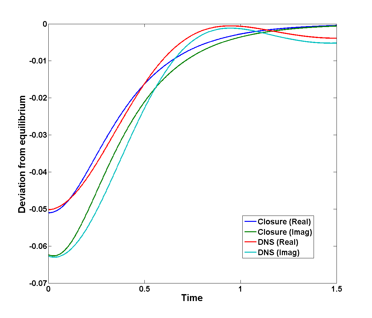
(a) Complex Mode 1

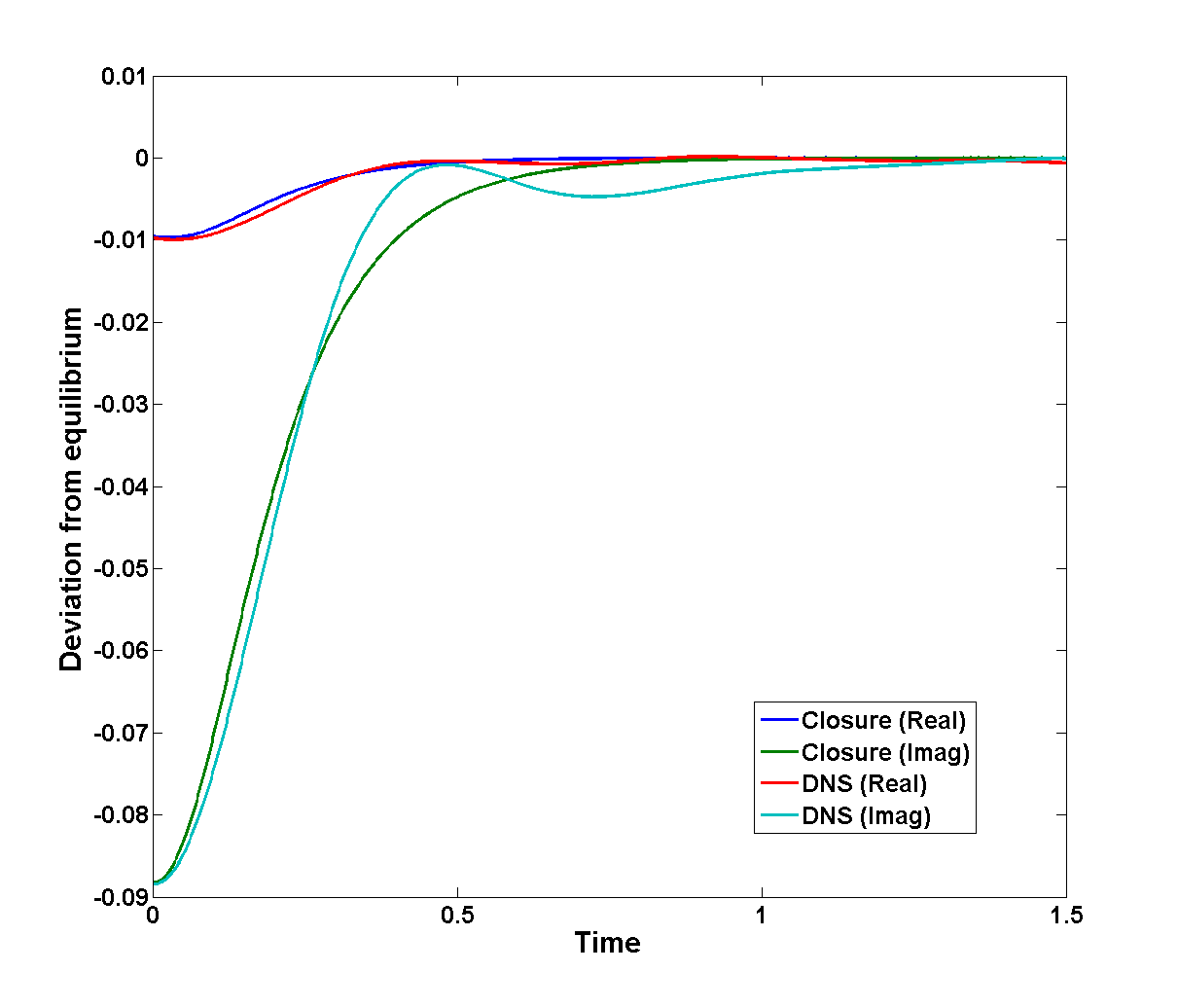
(b) Complex Mode 2

Figure 1: Comparison of the evolution of first moments for the direct numerical simulation (DNS) and the closure model. The initial conditions here are close to equilibrium (see text). There are five panels corresponding to the five retained complex modes of lowest wavenumbers. In each panel the real and imaginary part of each complex mode is plotted for both the DNS and closure. As usual both components of the complex modes have the same wave number.

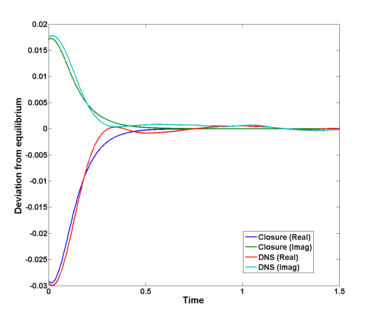
(a) Complex Mode 3

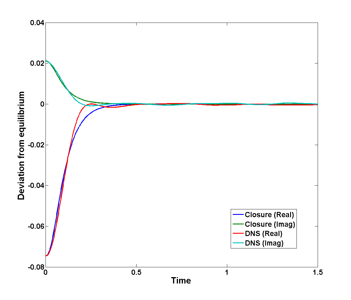
(b) Complex Mode 4

Figure 2: (continued)

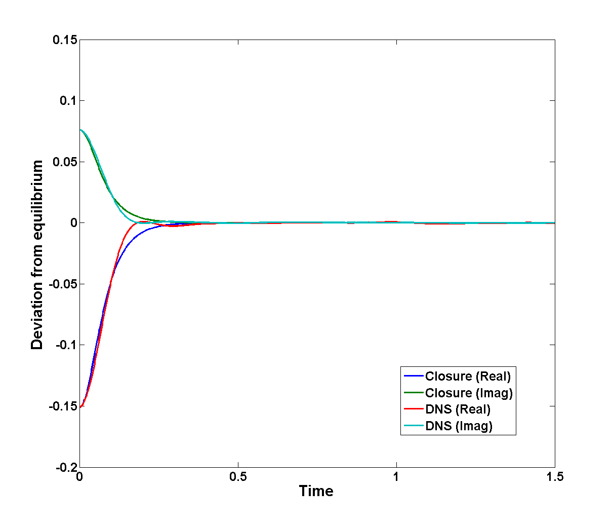
(a) Complex Mode 5

Figure 3: (continued)

8.1 Close to equilibrium case

A comparison between the first moments calculated by the DNS and those calculated using the closure model with the best choice of $\gamma=64.74$ is displayed in Figure 3. Overall the RMS error per mode per timestep is found to be $0.002035$, which may compared with the amplitude of the first moments. Each panel shows the behavior of the real and imaginary parts of $a_{k}(t)$ and all $m=5$ closure modes and DNS modes are plotted. The performance is quite good, and in particular two distinctive features of the statistical dynamics are well simulated qualitatively by the closure:

1. The DNS equilibration time for each complex mode is very clearly proportional to wavenumber and excellently reproduced by the closure equations. This provides strong evidence that the correct dissipation for reduced models of TBH is given by a fractional diffusion process. It is notable that exactly this kind of dissipation is the bare minimum required by the infinite Fourier mode Burgers-Hopf equation to prevent the appearance of a singular shock in finite time [17]. The optimal value of $\gamma$ reported above corresponds with an exponential damping time of $0.2779/|k|$, according to the simplified analysis at the beginning of Section 5, and this timescale is clearly visible in the approach to equilibrium of all modes.

2. Each mode exhibits essentially two well-defined regimes during equilibration: An initial “plateau” period and a later exponential decay to equilibrium. These periods are of comparable duration and are both directly proportional to wavenumber. Both of these features are predicted by the theoretical analysis of Section 6 and are readily apparent in Figure 3, most obviously for the low wavenumber cases. As the theoretical analysis shows, the fractional diffusion is ramping up during the plateau period, suggesting that the evolution of the resolved variables is more under the control of the initial conditions and to a lesser extent the non-linear interactions.

The discrepancy between DNS and closure tends, in general, to increase with time and is also more apparent in the low wavenumber modes. The DNS exhibits some oscillatory behaviour as it approaches equilibrium, which the closure model does not reproduce. These oscillations have a wavelength inversely proportional to the mode wavenumber. Nonetheless, a careful inspection reveals that the closure trajectories tend to “bisect” these DNS oscillations cleanly in every instance.

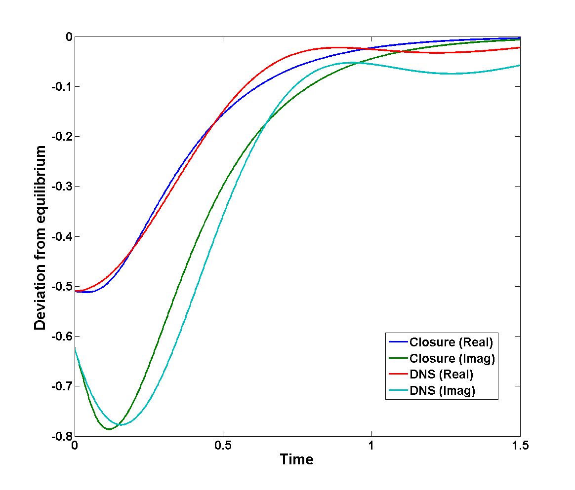
(a) Complex Mode 1

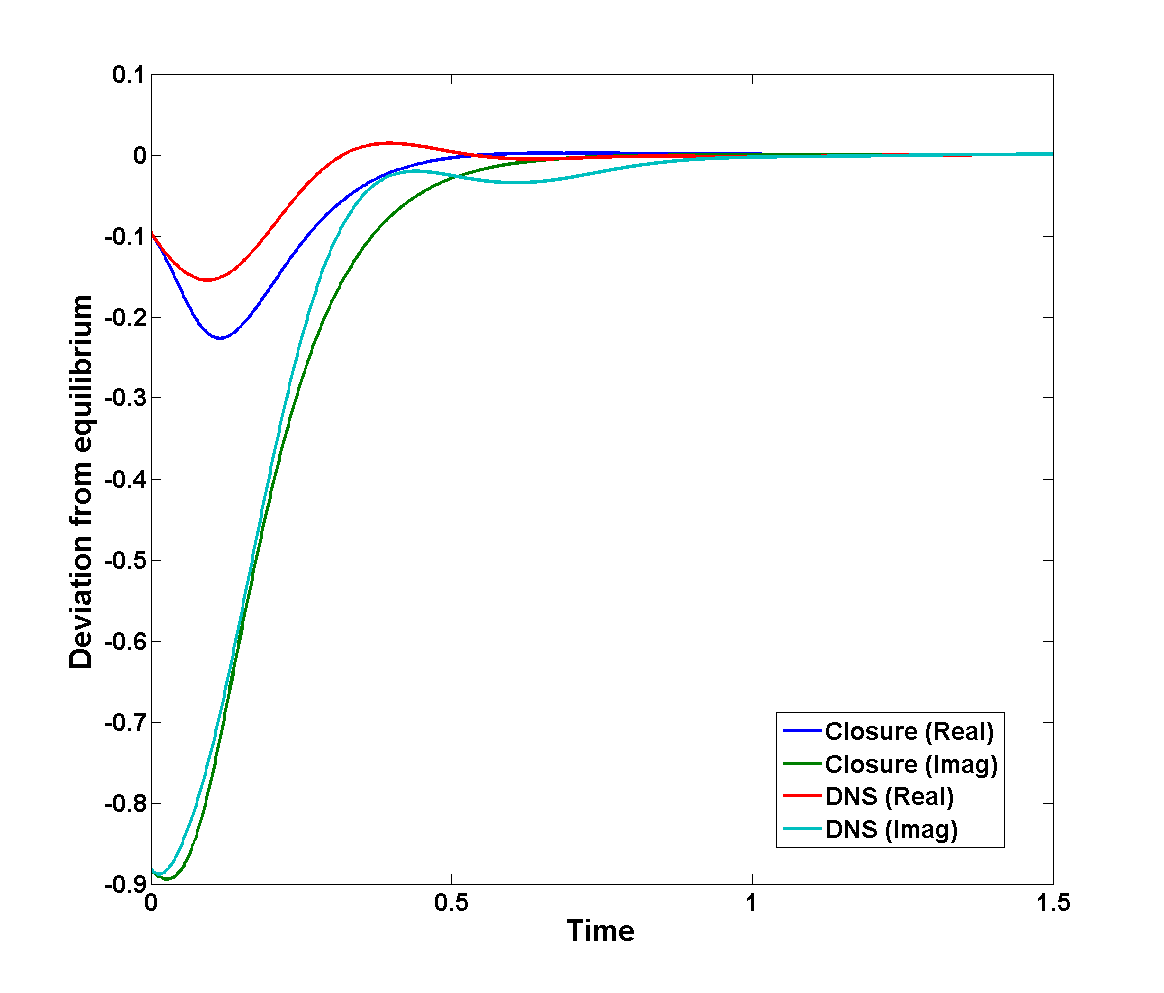
(b) Complex Mode 2

Figure 4: Same as Figure 3 except the initial conditions here are significantly removed from equilibrium (see text)

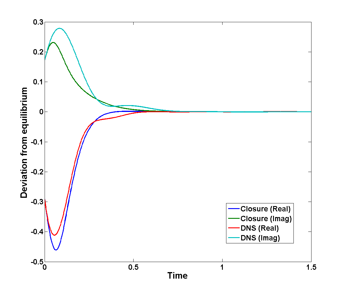
(a) Complex Mode 3

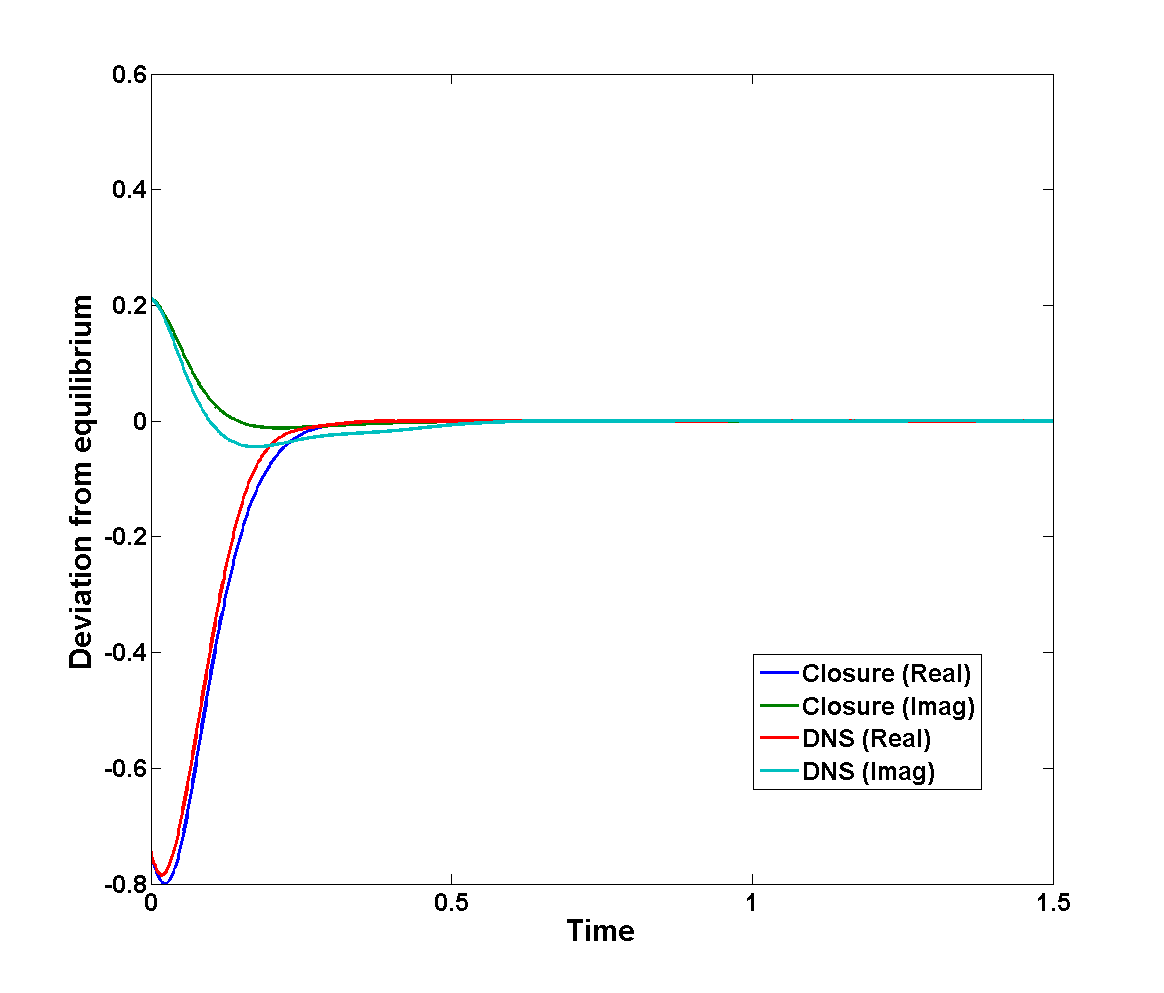
(b) Complex Mode 4

Figure 5: (continued)

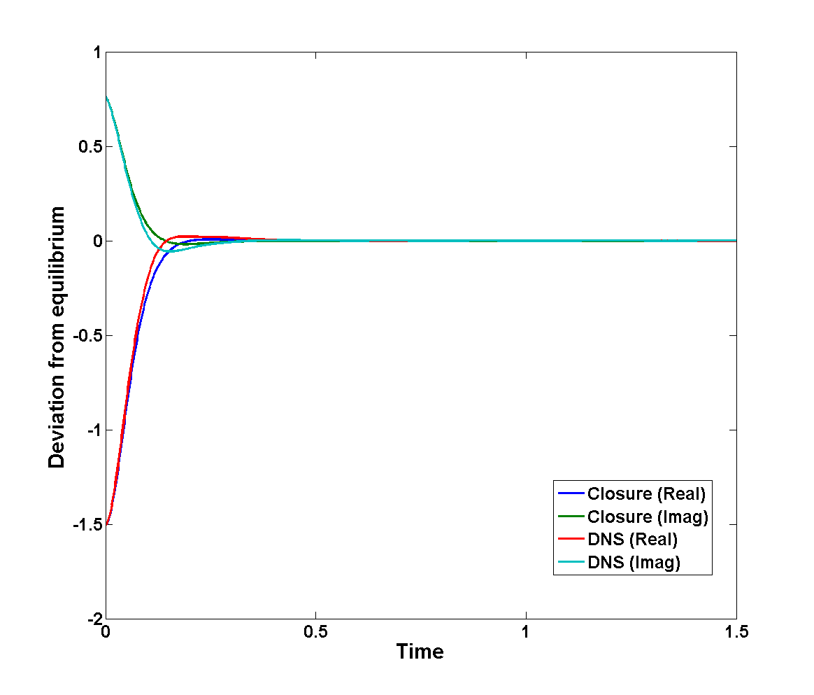
(a) Complex Mode 5

Figure 6: (continued)

8.2 Significantly removed from equilibrium case

Historically, closures theories have tended to be more successful in situations that are near statistical equilibrium. In the previous subsection our comparisons used initial mean deviations smaller than a typical equilibrium excursion of the system, namely, $1/\sqrt{2\beta}$ for each real mode. We now, therefore, pose a more stringent test of the closure to examine the case significantly removed equilibrium behavior. For simple expediency we multiply all deviations in the initial mean resolved variables by a factor of $\sqrt{10}$, the $r_{dev}$ parameter. The initial condition amplitudes are therefore an order of magnitude larger than the first experiment. This amplification also emphasizes the contribution of the quadratic advection terms in the closure equations. The results are displayed in Figure 6 in the same format as Figure 3. The best choice tunable parameter in this case is found to be $\gamma=73.83$, which corresponds to an exponential damping time of $0.2602/|k|$. The RMS error per mode and time step is $0.02561$ in this instance. Since all curves have been scaled up by a factor of $10$, this magnitude of error indicates that the fit is approximately 25% worse than in the close to equilibrium case.

The general behavior of the DNS equilibration is fairly similar to the close to equilibrium case, but with some notable differences. In particular, the general equilibration time scale is very much the same as the close to equilibrium case, again reinforcing the success of the reduced model with fractional diffusion. The primary difference is in the plateau period, during which larger differences between the closure and the DNS are evident, particularly for the lowest two wavenumbers (Figures 4(a) and 4(b)). This deviation suggests that the modification of the advection terms in the closure model is somewhat less successful than the robust prediction of effective, fractional diffusion.

8.3 Other initial condition deviations from equilibrium

We also examined the case $r_{dev}=1$ which lies midway between the choices considered above. Results are qualitiatively very similar (and indeed slightly improved) over the close to equilibrium case. The best choice for damping time here was $0.28156/|k|$ which is little removed from the close to equlibrium case considered above.

In contrast the case $r_{dev}=10$ produces poor results. This, of course, corresponds with a very large, ten standard deviation, excursion from equilibrium. The RMS error per mode and time step is $0.235$ and this is around four times what a simple rescaling of the results above would suggest. In addition the best fit damping time was dramatically shortened to $0.13805/|k|$, about half what the previous three settings give. Qualitatively the results (not shown) had big discrepancies which were most apparent as the various modes approached equilibrium, when large oscillations in the DNS were not reproduced by the closure. Failure of the closure in this case is perhaps not a complete surprise given that a Taylor series expansion about equilibrium was used to solve the Hamilton-Jacobi equation (see Section 6).

8.4 Robustness of tuning parameter

The results above show that for the three settings, $r_{dev}=1/\sqrt{10}$, $r_{dev}=1$ and $r_{dev}=\sqrt{10}$, the damping time only varies by approximately $8\%$. Given that the amplitude had been increased by an order of magnitude, the small change in the single adjustable parameter $\gamma$ is a rather reassuring indication of the robustness of the closure theory. To illustrate this robustness further we set the adjustable parameter $\gamma$ for the significantly removed from equilibrium case to be equal to the best-fit parameter for the close to equilibrium case. The ensuing closure dynamics is exhibited in Figure 9, which should be compared with Figure 6.

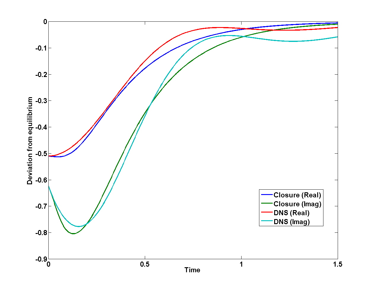
(a) Complex Mode 1

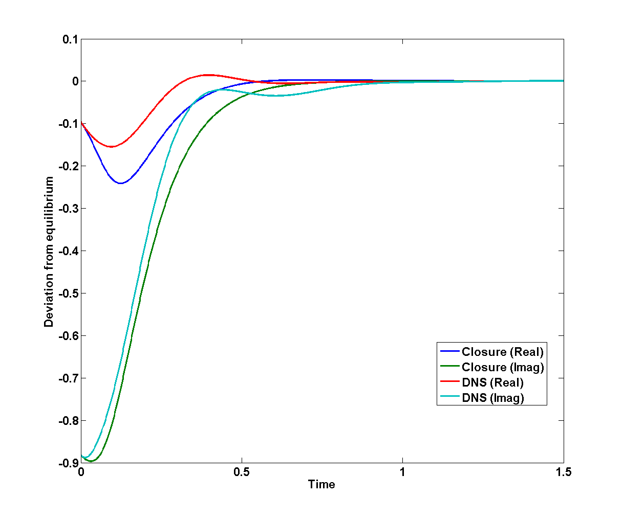
(b) Complex Mode 2

Figure 7: Same as Figure 6 except that the tuning parameter is set to that applying for Figure 3 (see text). This tests the robustness of the tuning parameter. This Figure should be compared with Figure 6.

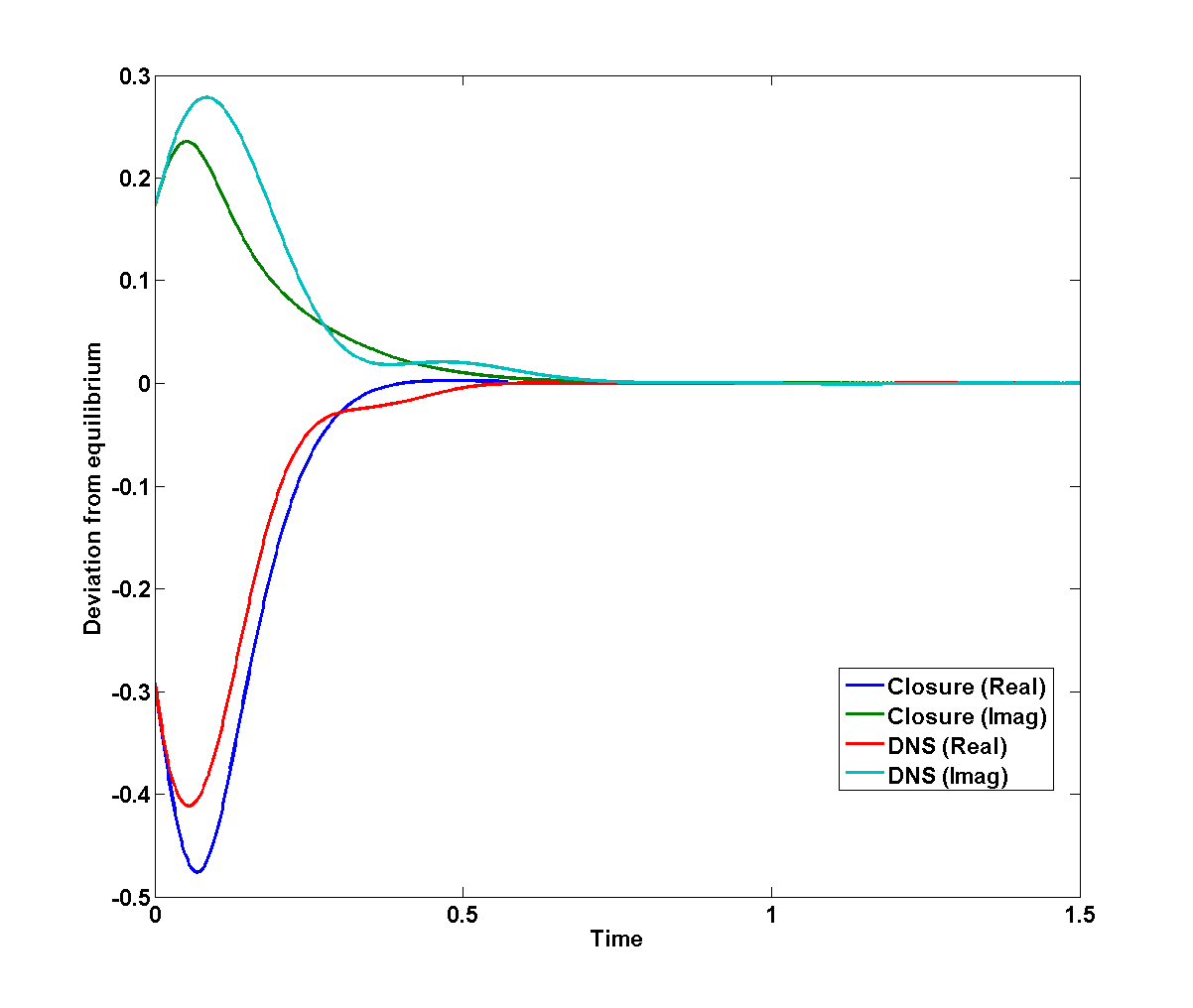
(a) Complex Mode 3

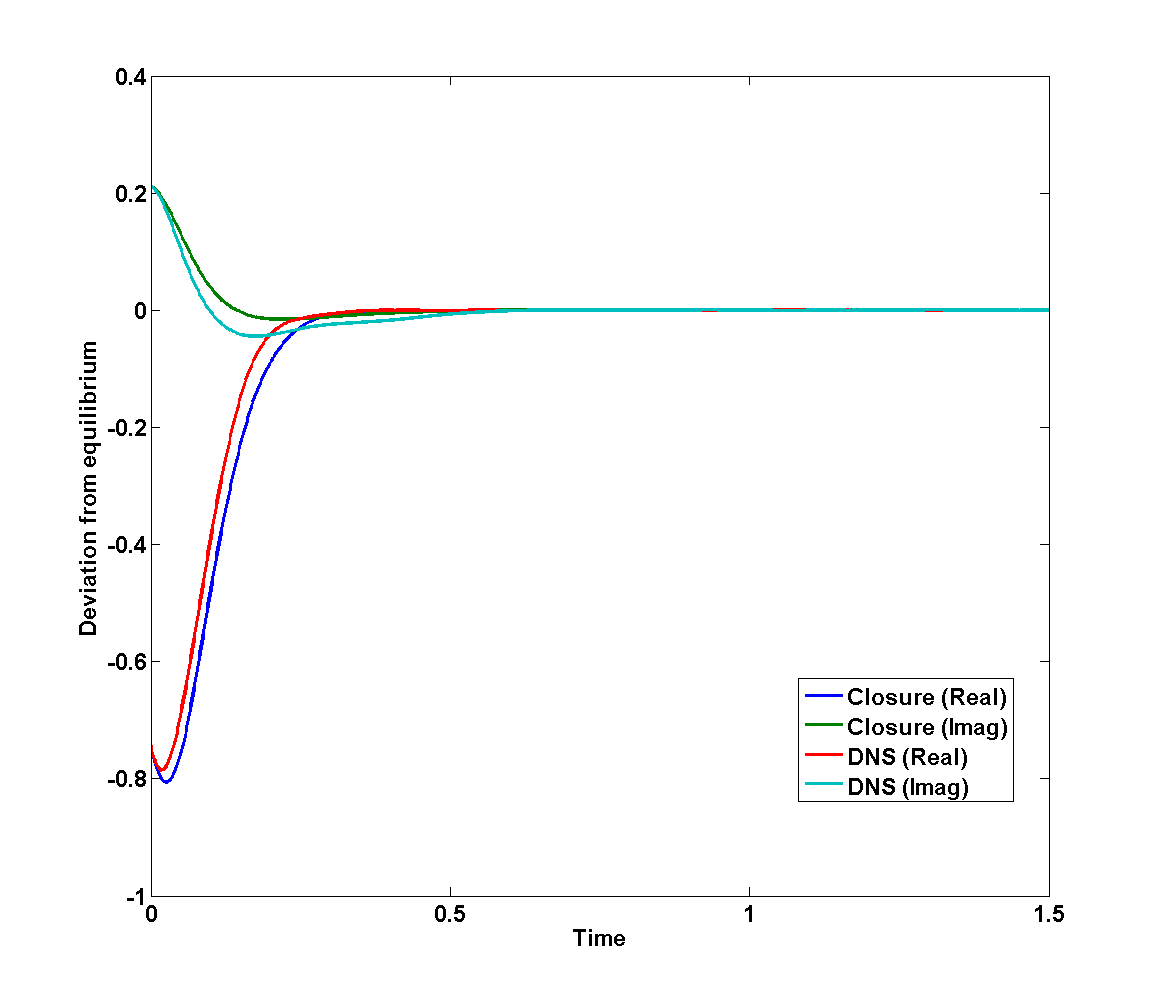
(b) Complex Mode 4

Figure 8: (continued)

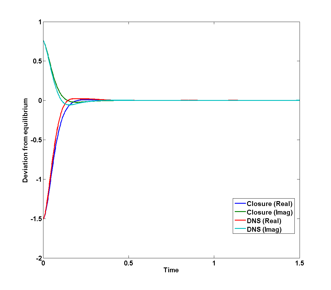
(a) Complex Mode 5

Figure 9: (continued)

8.5 A time scale separation experiment

As noted previously the system under study does not exhibit a clear separation of time scales between the slow, low wavenumber modes and the “neglected” fast, high wavenumber modes. Indeed, as shown in [27], this time scale is empirically observed to be inversely proportional to wave number, just like the dissipation time scale discussed above. Thus, for example, the second set of $2m$ modes have a time scale on average of only one third less than that of the last retained mode. This issue makes the construction of closure models for this system a challenge, as has been noted in detail in the stochastic mode reduction work of Majda, Vanden-Eijnden and collaborators (see [23]). Given this background it is reasonable to suspect that the discrepancies observed above, most notably for the significantly removed from equilibrium case, are due in part to time-scale separation issues. To test this idea in the context of our approach, we extend the closure model by incorporating an additional $2m$ “buffer” modes in the resolved variables, to separate the time scale of original closure modes from that of the neglected “heat bath” modes. In this new configuration the first unresolved mode has a time scale of one half of the last original resolved mode.

The buffered results for significantly removed from equilibrium initial conditions may be seen in Figure 12 in the same format as the previous two experiments. Interestingly, the best fit closure now exhibits a longer damping time of $0.3004/|k|$. This slower equilibration is perhaps explained by the inclusion of the buffer modes which mediate the nonlinear dissipation via the advection terms of the closure. The fit of the original modes is significantly improved relative to the unbuffered run, with the RMS error reduced to $0.0218$. Qualitatively, this improvement occurs most strikingly in the higher wavenumber modes $4$ and $5$ ,where the fit is now really quite impressive. This agreement might be expected since presence of the buffer modes removes the abrupt discontinuity in the original model at wavenumber $5$. There are also some smaller improvements with the low wave-number modes, especially in the plateau phase, but still the discrepancy with respect to the DNS oscillations on approach to equilibrium remains.

It is interesting to compare the results above to those in [24] where a stochastic reduction of the TBH system is proposed. These authors consider the case in which $m=1,2$ and assess performance using auto-correlation rather than first moment as is done here. In the near equilibrium case these are comparable due to the fluctuation dissipation relation. Like here they find that relaxation to equilibrium is exponential with a decay time given by the eddy turnover time. They also find the DNS oscillatory behaviour we observe and are also unable to produce it with their reduced model. They attribute this discrepancy to the lack of time separation between fast and slow modes. Our results with a significant buffer do not produce a large improvement in performance of the low wavenumber variables. This difference deserves closer future attention.

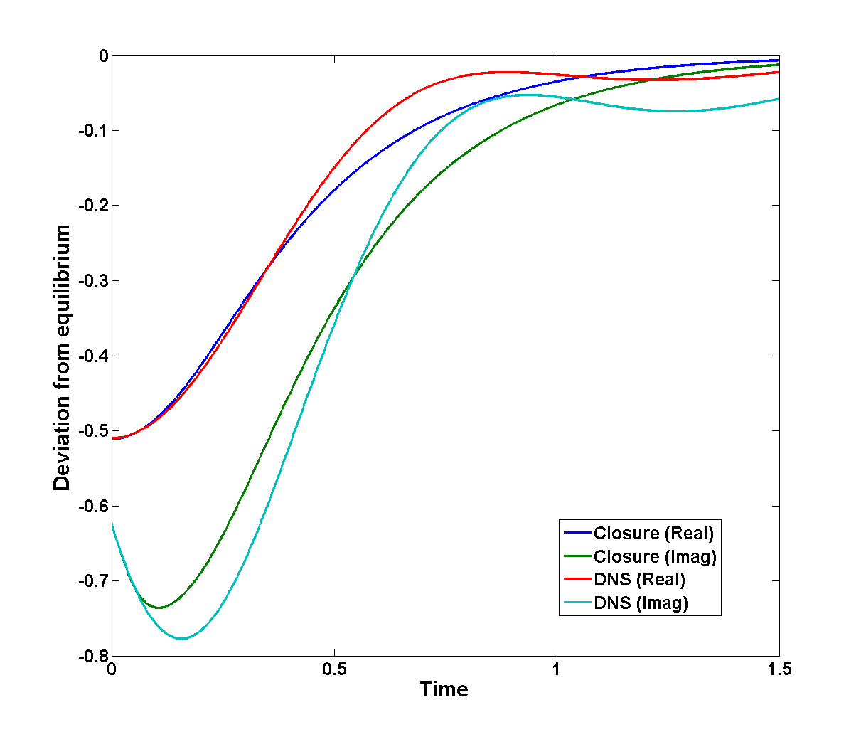
(a) Complex Mode 1

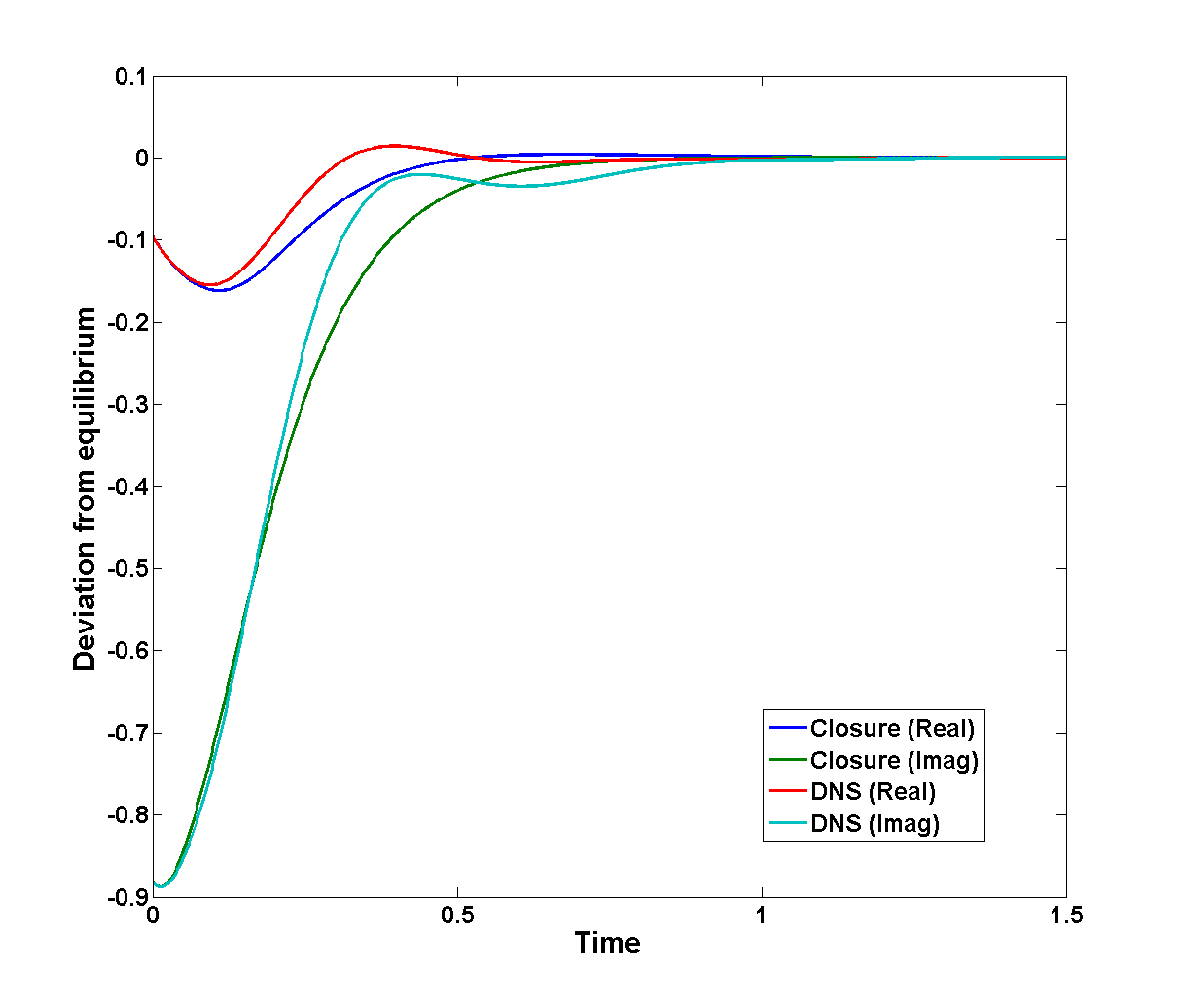
(b) Complex Mode 2

Figure 10: Same as Figure 6 except the closure model has an additional 5 complex ”buffer” modes (see text)

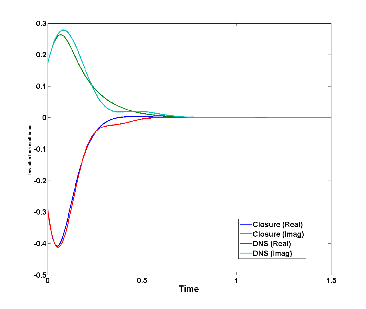
(a) Complex Mode 3

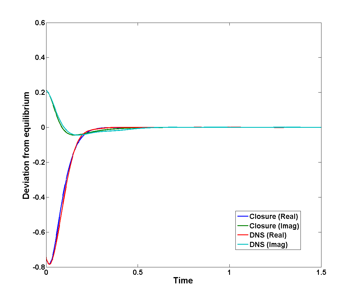
(b) Complex Mode 4

Figure 11: (continued)

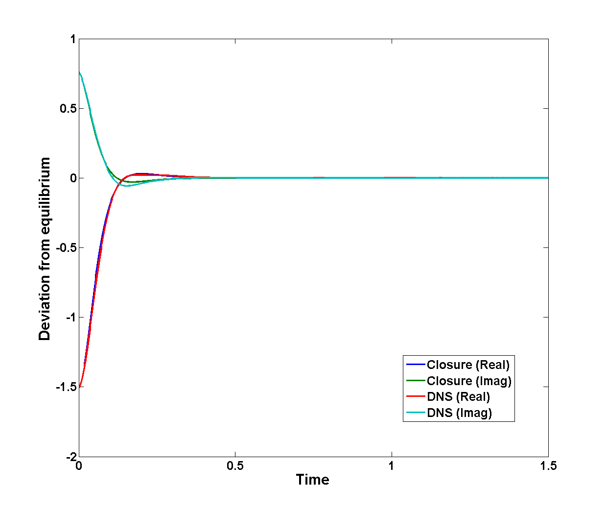
(a) Complex Mode 5

Figure 12: (continued)

9 Summary and Conclusions

A fundamental problem in nonequilibrium statistical mechanics, studies of turbulence and stochastic modelling of complex systems is the formulation of tractable reduced models of the slow, coherent part of the dynamical system. One of the authors has proposed a general variational principle for producing such closures in the context of Hamiltonian dynamics. This closure theory fits a continuous time series of trial probability densities to the Liouville equation using a weighted, time-integrated, mean-squared cost functional to quantify the lack-of-fit. The closed reduced equations satisfied by minimizers of the cost functional are then obtained by classical Hamilton-Jacobi theory. More details may be found in the companion paper [31].

In this contribution we have applied this closure theory to a Galerkin-truncated Burgers-Hopf model, which has been proposed as a simple analog of more complex and realistic fluid systems. The model is governed by a Hamiltonian dynamics, has a Gibbs invariant measure, and exhibits mode decorrelation with time scales that vary inversely with wavenumber. These properties make it an ideal testbed for future work with more realistic turbulent systems. In the present work we have concentrated on the free relaxation of the system from nonequilibrium statistical initial conditions.

Our results pertain to a reduced model for the lowest $5$ complex modes in a dynamical system of $50$ nonlinearly interacting complex modes. In light of the simplicity of the Gibbs measure, under which all the modes are independent Gaussians, it is possible to carry out the calculation of the governing equations for the reduced model explicitly up to second-order (quadratic nonlinearity) in the mean resolved variables. The result is a set of governing equations for the temporal evolution of the first moments of the resolved modes which resembles a severe truncation of original nonlinear system with the following modifications and characteristics.

1. There is a fractional dissipation which is proportional to the wavenumber of the mode. Remarkably this fractional diffusion is the minimum such regularization required to prevent finite-time singularities in the continuous (infinite mode) Burgers-Hopf system [17]. It is the primary mechanism by which the reduced model irreversibly equilibrates, and as expected by linear-response theory it has the same wavenumber-dependent time scale as the modal decorrelation time.

2. The nonlinear terms of the best-fit reduced model have modified coefficients which imply an altered energy flux between resolved modes compared with the original TBH system. By means of these coefficients the reduced model approximates the indirect influence of the unresolved modes on the interactions between the mean resolved modes.

3. Both these modifications of the dynamics are time-dependent in that they take a time comparable to the equilibration time to manifest themselves in full. This initial period, which we term the plateau time, is incorporated naturally in the nonstationary version of our closed reduced model.

The first-moment best-fit closure model has been compared with a direct numerical simulation (DNS) of the full TBH system using very large ensembles. The comparisons are generally good for a broad range of initial deviations from equilibrium. If however the deviation is made sufficiently large the fit does break down significantly. This is not surprising given that the closure equations rely on a Taylor expansion of the Hamilton-Jacobi equation centered on equilibrium.

The wavenumber-dependent equilibration time scale predicted by the best-fit closure matches that produced by the DNS across the spectrum of resolved modes. Only one scalar parameter is adjusted empirically to fit the closure predictions to the DNS results. The value of this parameter is observed to be quite robust even as the imposed nonequilibrium initial conditions are increased by an order of magnitude.

The TBH dynamics is a rather severe test for reduced models given that there is no clear separation of timescales. We have found that the performance of the reduced model can be improved by inserting some “buffer” modes, which widens the separation of time scales between the slow and fast parts of the system. Nonetheless, some slow oscillatory behavior of the low resolved modes is missed by the reduced model, indicating perhaps that there are memory effects inherent in the statistical dynamics. It is conceivable that an extended set of resolved variables that includes the time derivatives of the lowest modes might be able to capture those oscillations.

Given that the TBH dynamics has been developed as a paradigm for more complex dynamical systems having quadratic nonlinearities typical of hydrodynamical equations of motion, the question arises whether the methodology that we have applied in the present investigation could be extended to other systems. When coarse-graining complex systems of this type onto their low, slow modes, one may expect to encounter Liouville residuals having similar structure to that in the TBH case. Under such circumstances cost functions akin to the one that we have constructed in the TBH case, which quantify the collective effect of products of pairs of modes, may prove to be an efficacious way to represent the influence of unresolved fluctuations on the reduced dynamics. Future investigations on other systems of this kind exhibiting turbulent dynamics would be helpful in evaluating the range of applicability of our best-fit approach and the useful forms of the cost functions that define it. The reader is referred to [31] for some further discussion on these issues.

Appendix A Ancilliary Material

Here we collect some standard conventions and calculations concerning functions of several complex variables which may be useful to the reader a various points in the paper.

For any smooth, complex-valued function $f(z)$, of $n$ complex variables, $z=(z_{1},\ldots,z_{n})\in l\!\!\!C^{n}$, with $z_{k}=x_{k}+iy_{k}$, the usual derivatives are defined by

$$\frac{\partial f}{\partial z_{k}}=\frac{1}{2}\left(\,\frac{\partial f}{\partial x_{k}}-i\frac{\partial f}{\partial y_{k}}\,\right)\,,\;\;\;\;\;\;\;\;\frac{\partial f}{\partial z_{k}^{*}}=\frac{1}{2}\left(\,\frac{\partial f}{\partial x_{k}}+i\frac{\partial f}{\partial y_{k}}\,\right)\,;$$

the notation $z_{k}^{*}=x_{k}-iy_{k}$ is used for complex conjugate. In terms of these, the chain rule for the composite function $f(z(t))$, where $t$ is a real variable, is simply

$$\frac{d}{dt}f(z(t))=\sum_{k=n}^{n}\frac{\partial f}{\partial z_{k}}\frac{dz_{k}}{dt}+\frac{\partial f}{\partial z_{k}^{*}}\frac{dz_{k}^{*}}{dt}\,=\,\sum_{k=-n}^{n}\frac{\partial f}{\partial z_{k}}\frac{dz_{k}}{dt}\,.$$

The last equality uses the convention that $z_{-k}=z_{k}^{*}$, which occurs naturally in the context of a Fourier representation of a dynamics in terms of complex amplitudes $z_{k}$.

Repeated application of this chain rule to the function $f(tz)$, $0\leq t\leq 1$, yields the complex form of Taylor’s expansion,

$$f(z)=f(0)+\sum_{k=-n}^{n}L_{k}\,z_{k}+\sum_{k_{1},k_{2}=-n}^{n}M_{k_{1}k_{2}}\,z_{k_{1}}z_{k_{2}}+\sum_{k_{1},k_{2},k_{3}=-n}^{n}N_{k_{1}k_{2}k_{3}}\,z_{k_{1}}\,z_{k_{2}}z_{k_{3}}+O(|z|^{4})\,,$$

with coefficients

$$L_{k}=\frac{\partial f}{\partial z_{k}}(0)\,,\;\;\;\;M_{k_{1}k_{2}}=\frac{1}{2}\frac{\partial^{2}f}{\partial z_{k_{1}}\partial z_{k_{2}}}(0)\,,\;\;\;\;N_{k_{1}k_{2}k_{3}}=\frac{1}{6}\frac{\partial^{3}f}{\partial z_{k_{1}}\partial z_{k_{2}}\partial z_{k_{3}}}(0)\,.$$

In Section 5 this expansion is used to determined an approximation to the value function, $v(\lambda)$, for $\lambda\in l\!\!\!C^{m}$, and in Section 6 for the time-dependent value function $v(\lambda,t)$. For those calculations this form of the expansion is better than the equivalent multi-index form.

The Lagrangian ${\mathcal{L}}(\lambda,\dot{\lambda})$ and the Hamiltonian ${\mathcal{H}}(\lambda,\mu)$ that occur in the defining optimization principle and the associated Hamilton-Jacobi equation, respectively, are related by the Legendre tranform (25). It is instructive to relate this complexified Legendre transform to the familiar real transform. Write the complex variables as $\lambda_{k}=\xi_{k}+i\eta_{k}$ and $\mu_{k}=\phi_{k}+i\psi_{k}$, for $k=1,\ldots,m$. Then, (25) is equivalent to

$$\phi_{k}=\frac{\partial}{\partial\dot{\xi}_{k}}\,\frac{{\mathcal{L}}}{2}\,,\;\;\;\;\psi_{k}=\frac{\partial}{\partial\dot{\eta}_{k}}\,\frac{{\mathcal{L}}}{2}\,,\;\;\;\;\frac{{\mathcal{H}}}{2}=\sum_{k=1}^{m}\phi_{k}\dot{\xi}_{k}+\psi_{k}\dot{\eta}_{k}\,-\,\frac{{\mathcal{L}}}{2}\,.$$

Thus the complex Legendre transform (25) between ${\mathcal{L}}$ and ${\mathcal{H}}$ is identical with the real tranform between ${\mathcal{L}}/2$ and ${\mathcal{H}}/2$. The stationary value function, $v(\lambda)$, in (17) is defined by the action integral for ${\mathcal{L}}(\lambda,\dot{\lambda})$ and satisfies the complex form of the Hamilton-Jacobi equation (26). The conjugacy relation (27) determined by $v$ is

$$\mu_{k}=-\frac{\partial v}{\partial\lambda_{k}^{*}}(\lambda)=-\left[\,\frac{\partial}{\partial\xi_{k}}+i\frac{\partial}{\partial\eta_{k}}\,\right]\frac{v}{2}\,,$$

This relation shows that (26) and (27) are identical with the real Hamilton-Jacobi theory applied to the Hamiltonian ${\mathcal{H}}(\xi,\eta,\phi,\psi)/2$ and the value function $v(\xi,\eta)/2$. The nonstationary case is complexified in the same way. The common factor of $1/2$ throughout is irrelevant to the analysis, being absorbed in the complex variable conventions.

In the course of this work the authors benefited from conversations with A. J. Majda and E. Vanden Eijnden. Part of this research was completed during B.T.’s two-month visit to the Courant Institute of Mathematical Sciences in Spring 2012. The authors also acknowledge the use of the Burgers-Hopf numerical model code authored by I. Timofeyev.

References

- [1] Abramov, R.; Kovacic, G.; Majda, A. Hamiltonian structure and statistically relevant conserved quantities for the truncated Burgers-Hopf equation. Communications on pure and applied mathematics 56 (2003), no. 1, 1–46.
- [2] Arnol’d, V. I. Mathematical methods of classical mechanics, Springer-Verlag, New York, 1989.
- [3] Balescu, R. Equilibrium and nonequilibrium statistical mechanics, Wiley, New York, 1975.
- [4] Bryson, A. E.; Ho, Y.-C. Applied optimal control: Optimization, estimation, and control, Hemisphere Pub. Corp.(Washington and New York), 1975.
- [5] Casella, G.; Berger, R. L. Statistical inference, Duxbury Press, 2001.
- [6] Chandler, D. Introduction to modern statistical mechanics, Oxford University Press, 1987.
- [7] Chorin, A. J.; Hald, O. H.; Kupferman, R. Optimal prediction and the Mori–Zwanzig representation of irreversible processes. Proc. Nat. Acad. Sci. 97 (2000), no. 7, 2968–2973.
- [8] Chorin, A. J.; Hald, O. H.; Kupferman, R. Optimal prediction with memory. Physica D: Nonlinear Phenomena 166 (2002), no. 3, 239–257.
- [9] Chorin, A. J.; Kast, A. P.; Kupferman, R. Optimal prediction of underresolved dynamics. Proc Nat. Acad. Sci. 95 (1998), no. 8, 4094–4098.
- [10] De Groot, S. R.; Mazur, P. Non-equilibrium thermodynamics, North Holland, 1962.
- [11] Evans, L. C. Partial differential equations. graduate studies in mathematics 19. American Mathematical Society (1998).
- [12] Fleming, W. H.; Rishel, R. W. Deterministic and stochastic optimal control, vol. 268, Springer-Verlag New York, 1975.
- [13] Gelfand, I. M.; Fomin, S. V. Calculus of variations, Dover publications, 2000.
- [14] Givon, D.; Kupferman, R.; Stuart, A. Extracting macroscopic dynamics: model problems and algorithms. Nonlinearity 17 (2004), no. 6, R55.
- [15] Katz, A. Principles of statistical mechanics: the information theory approach, WH Freeman, 1967.
- [16] Keizer, J. Statistical thermodynamics of nonequilibrium processes, Springer, 1987.
- [17] Kisalev, A.; Nazaraov, F.; Shterenberg, R. Blow up and regularity for fractal Burgers equation. pre-print (2008). ArXiv:0804.3549.
- [18] Kleeman, R.; Majda, A. J.; Timofeyev, I. Quantifying predictability in a model with statistical features of the atmosphere. Proc. Nat. Acad. Sci. USA 99 (2002), 15 291–15 296.
- [19] Kullback, S. Information theory and statistics, Dover publications, 1997.
- [20] Lanczos, C. The variational principles of mechanics, Dover Publications, 1986.
- [21] Lax, P. D. Hyperbolic systems of conservation laws ii. Selected Papers Volume I (2005), 233–262.
- [22] Luzzi, R.; Vasconcellos, Á. R.; Ramos, J. G. Predictive Statistical Mechanics: A Nonequilibrium Ensemble Formalism, Springer, 2002.
- [23] Majda, A.; Timofeyev, I.; Vanden-Eijnden, E. A priori tests of a stochastic mode reduction strategy. Physica D 170 (2002), 206–252.
- [24] Majda, A.; Timofeyev, I.; Vanden-Eijnden, E. Stochastic models for selected slow variables in large deterministic systems. Nonlinearity 19 (2006), no. 4, 769.
- [25] Majda, A. J.; Harlim, J.; Gershgorin, B. Mathematical strategies for filtering turbulent dynamical systems. Discrete and Continuous Dynamical Systems 27 (2010), no. 2, 441–486.
- [26] Majda, A. J.; Timofeyev, I. Remarkable statistical behavior for truncated Burgers-Hopf dynamics. Proc. Nat. Acad. Sci. USA 97 (2000), 12 413–12 417.
- [27] Majda, A. J.; Timofeyev, I. Statistical mechanics for truncations of the Burgers-Hopf equation: a model for intrinsic stochastic behavior with scaling. Milan Journal of Mathematics 70(1) (2002), 39–96.
- [28] Majda, A. J.; Timofeyev, I.; Vanden-Eijnden, E. A mathematics framework for stochastic climate models. Comm. Pure Appl. Math. 54 (2001), 891–974.
- [29] Öttinger, H. C. Beyond equilibrium thermodynamics, Wiley-Interscience, 2005.
- [30] Sagan, H. Introduction to the Calculus of Variations, Dover Publications, 1992.
- [31] Turkington, B. An optimization principle for deriving nonequilibrium statistical models of Hamiltonian dynamics. pre-print (2012). ArXiv:1207.2692.
- [32] Zubarev, D. N. Nonequilibrium Statistical Thermodynamics, Plenum Press, New York, 1974.
- [33] Zwanzig, R. Nonequilibrium statistical mechanics, Oxford University Press, USA, 2001.