The Ising antiferromagnet on an anisotropic simple cubic lattice in the presence of a magnetic field

Abstract

We have studied the anisotropic three-dimensional nearest-neighbor Ising model with competitive interactions in an uniform longitudinal magnetic field $H$. The model consists of ferromagnetic interaction $J_{x}(J_{z})$ in the $x(z)$ direction and antiferromagnetic interaction $J_{y}$ in the $y$ direction. We have compared our calculations within a effective-field theory in clusters with four spins (EFT-4) in the simple cubic (sc) lattice with traditional Monte Carlo (MC) simulations. The phase diagrams in the $h-k_{B}T/J_{x}$ plane ($h=H/J_{x}$) were obtained for the particular case $\lambda_{1}=J_{y}/J_{x}(\lambda_{2}=J_{z}/J_{x})=1$ (anisotropic sc). Our results indicate second-order frontiers for all values of $H$ for the particular case $\lambda_{2}=0$ (square lattice), while in case $\lambda_{1}=\lambda_{2}=1$, we observe first- and second-order phase transitions in the low and high temperature limits, respectively, with presence of a tricritical point. Using EFT-4, a reentrant behavior at low temperature was observed in contrast with results of MC.

I Introduction

In recent years, the effect of a longitudinal field in the Ising antiferromagnet on an anisotropic simple cubic (sc) lattice has been discussed. The experimental example is compound $(C_{2}H_{5}NH_{3})_{2}CuCl_{4}$ dejongh . The differential magnetic susceptibility $\chi=\left(\frac{\partial M}{\partial H}\right)_{T}$ of this compound was analysed as a function of an extra external field ($0-2$ kOe) and of temperature ($1-30$ K; $T_{c}=10.20$ K). The compound is a typical layer-type ferromagnet, with a very weak antiferromagnetic coupling between the $Cu^{2+}$ layers, where has been established the magnetic phase diagram of the antiferromagnetic structure. One of the attractive points of investigating the properties of $(C_{2}H_{5}NH_{3})_{2}CuCl_{4}$ is that as a consequence of the antiferromagnetic interlayer coupling we may obtain quantitative information about the anisotropy and $J_{AF}$ (exchange coupling) by investigating the field dependence of the susceptibility at $T<T_{c}$. In previous papers dejongh2 ; bloembergen ; dejongh3 ; miedema it has been reported that the $Cu$ compounds of general formula $(C_{n}H_{2n+1}NH_{3}CuX_{4})$, where $n=1$, $2$, $3$, $4$, $5$, $6$, $10$ and $X=Cl$ or $Br$, may be considered as consisting of nearly isolated magnetic layers. Other example of the compound with cubic anisotropy are antiferromagnet $K_{2}MnF_{4}$ mulder , $(CH_{3}NH_{3})_{2}MnCl_{4}$ and $(CD_{3}ND_{3})_{2}MnCl_{4}$ heger .

Three dimensional (3D) Ising models and (pseudo-) Ising physical systems have been analysed extensively domb ; wolf . Graim and Landau graim studied the critical behavior of a spin-$1/2$ Ising model on a simple cubic lattice with spatially anisotropic nearest-neighbor coupling using the Monte Carlo method. This model on an anisotropic square lattice was investigated by using a modified mean-field theory in which the intrachain is treated exactly and the interactions between chains are considered in the mean-field theory stout ; hone ; sato . Various approximate methods have show this critical bahavior of the curve $T_{N}$ versus $H$, such as mean field approximation (MFA) garrett ; ziman , effective-field theory (EFT) zukovic , mean field renormalization group (MFRG) slotte , effective-field renormalization group (EFRG) neto2004 , Monte Carlo simulation (MC) landau ; landau1976 ; ferrenberg , and high-temperature series expansion (SE) bienenstock . For the case of the 3D lattice, the theoretical calculations show disagreement between differente methods. The results obtained by the MFA and EFT methods show a reentrant behavior in the phase diagram in low-temperature, i.e., if $H$ is just above $H_{c}$, then these are two phase transitions as the temperature is increased.

In recent years, the effect a longitudinal field in the Ising antiferromagnetic on an anisotropic square lattice was explored by MC viana2009 . Although MC simulations play an important role for the study of phase transitions and critical phenomena, the well-known difficulties arise when one uses standard algorithms (one-flip algorithms) metropolis for the study of first-and second-order phase transitions. This has contributed for the development of alternative MC methods, such as parallel-tempering nemoto , cluster algorithms wolff , multicanonical algorithms berg , and more recently Wang-Landau method wanglandau .

In the present paper we use the MC simulations and effective-field theory in clusters with four spins (EFT-4). We investigate the first- and second-order phase transition in the plane $h-k_{B}T/J_{x}$ of the Ising superantiferromagnet on an anisotropic simple cubic lattice in the presence of a magnetic field. Standard finite-size scaling techniques were used to estimate the critical temperatures. In Section II we present the model and formalism. The numerical results and discussions are given in Section III. Finally, the last section is devoted to conclusions.

II Model and Formalism

II.1 Hamiltonian

The model in this work is the nearest-neighbor ($nn$) Ising antiferromagnetic in a longitudinal field magnetic divided into two equivalent interpenetrating sublattices $A$ e $B$, that is described by following Hamiltonian

$$\mathcal{H}=-J_{x}\sum\limits_{i,\overrightarrow{\delta_{x}}}\sigma_{i}^{z}\sigma_{i+\overrightarrow{\delta_{x}}}^{z}+J_{y}\sum\limits_{i,\overrightarrow{\delta_{y}}}\sigma_{i}^{z}\sigma_{i+\overrightarrow{\delta_{y}}}^{z}-J_{z}\sum\limits_{i,\overrightarrow{\delta_{z}}}\sigma_{i}^{z}\sigma_{i+\overrightarrow{\delta_{z}}}^{z}-H\sum\limits_{i}\sigma_{i}^{z},$$ (1)

where $\sigma_{i}^{\mu}$ is the $\mu(=x,y,z)$ component spin-$1/2$ Pauli operator at site $i$, $J_{x}(J_{y},J_{z})$ is the exchange coupling along the $x(y,z)$ axis, $\delta_{x}(\delta_{y},\delta_{z})$ denotes the nearest-neighbor vector along the $x(y,z)$ axis and $H$ is the longitudinal magnetic field. We define the parameters $\lambda_{1}=J_{y}/J_{x}$ and $\lambda_{2}=J_{z}/J_{x}$. The ordered state for low temperatures and fields is the superantiferromagnetic order (SAF), which is characterrized by a parallel spin orientation in horizontal direction and an antiparallel spin orientation of a parallel spin orientation of nearest-neighbors in vertical direction and therefore exhibit Néel order within the initial sublattice $A$ and $B$ (see figure (1)).

If $\lambda_{2}=0$ ($J_{z}=0$), the lattice is now composed of independent planes, so the model is exactly solved for $H=0$, and the critical temperature is obtained by the following relation onsager

$$\sinh\left(\frac{2J_{x}}{k_{B}T_{N}}\right)\sinh\left(\frac{2J_{y}}{k_{B}T_{N}}\right)=1,$$ (2)

where for the particular isotropic case $J_{x}=J_{y}=J$ ($\lambda_{1}=1$ ) we have $k_{B}T_{N}/J=2/\ln(1+\sqrt{2})$. For $H\neq 0$, with $\lambda_{1}\neq 1$, $\lambda_{1}=1$ we have an Ising model with an external magnetic field on an anisotropic square lattic (1), which was already studied by MC viana2009 . Accordingly, we improve the understanding of this model by studying it by means of the Effective-Field Theory and Monte Carlo simulations for the case $\lambda_{1}=\lambda_{2}$ and $H\neq 0$.

II.2 Monte Carlo Simulation

In order to implement the present model to perform MC by the Metropolis Algorithm, the simple cubic lattice of size $L$ having $L\times L\times L$ sites is decomposed into two sublattices ($A$ and $B$) with opposite spins, corresponding to the SAF ground state. To meassure the SAF order, the appropriate order parameter is defined by $\left\langle m_{s}\right\rangle=\left\langle(m_{A}-m_{B})/2\right\rangle$, where $\left\langle m_{\mu}\right\rangle=\left\langle\frac{2}{N}\sum_{i\in\mu}\sigma_{i}\right\rangle$ is the magnetization of the sublattice $\mu=A$, $B$ and $N=L^{3}$ number of spins. The susceptibility related to this order parameter is defined as follows:

$$\chi=L^{d}(\langle m_{s}^{2}\rangle-{\langle m_{s}\rangle}^{2})/T,$$ (3)

where $d$ is the dimension of the lattice.

In our simulations we have considered lattices with periodic boundary conditions. In order to determine the system’s behavior in the thermodynamic limit ($L\rightarrow\infty$), which is imposible to implement on account of computational limitation, we have to use a finite-size scaling theory fisher . Accordingly, to locate the critical temperature for second-order phase transitions, we approximately locate the crossing point of curves for different sizes of the fourth-order cumulant $U_{4}(L)$ (Binder Cumulant) defined as binder

$$U_{4}(L)=1-\frac{\left\langle m_{s}^{4}\right\rangle}{3\left\langle m_{s}^{2}\right\rangle^{2}},$$ (4)

where $\left\langle m_{s}^{2}\right\rangle$ and $\left\langle m_{s}^{4}\right\rangle$ are the canonical averages of the second and fourth moments of magnetization, respectively. On the other hand, the critical temperature $T_{c}$ can also be obtained by means of the relation $T_{c}^{L}=T_{c}+aL^{-1/\nu}$, where $T_{c}^{L}$ is the pseudocritical temperature corresponding to the size $L$, and $\nu$ is the correlation critical exponent. For first-order phase transitions the same formula applies by setting $1/\nu=d$. A more extensive description of the Monte Carlo method was published elsewhere landau1976 and the reader is referred there for further details. We performed simulations for $\lambda_{1}=\lambda_{2}$, for several values of $h$, with a temperature step $\Delta T=0.01$ and runs comprising up to $2\times 10^{5}$ MC steps after equilibration. The statistical errors of the MC simulations used for the estimation of $T_{N}(\lambda_{1},\lambda_{2},h)$ of a particular $\lambda_{1}$, $\lambda_{2}$ and $h=H/J_{x}$ were found much smaller than the statistical errors coming from the fact that we used. Therefore, the error bars are not shown in our graphs because they are smaller than the symbol sizes.

II.3 Effective-Field Theory

As a starting point, the averages of a general function involving spin operator components $O(\{n\})$ are obtained by denise

$$\left\langle\mathcal{O}(\{n\})\right\rangle=\left\langle\frac{\text{Tr}{\{n\}}\mathcal{O}(\{n\})e^{-\beta\mathcal{H}_{\{n\}}}}{Tr_{\{n\}}e^{-\beta\mathcal{H}_{\{n\}}}}\right\rangle,$$ (5)

where the partial trace Tr_{n} is taken over the set $\{n\}$ of spin variables (finite cluster) specified by the multisite spin Hamiltonian $H_{\{n\}}$ and $\left\langle\cdot\cdot\cdot\right\rangle$ indicates the usual canonical thermal average.

The method treats the effects of the surrounding spins of a finite cluster with $N$ spins through a convenient differential operator technique honmura such that, in contrast to the usual MFA procedure, all relevant self-spin correlations are taken exactly into account. The interactions within the cluster are exactly treated and the effect of the remaining lattice spins is treated by a given approximation (here we use the random phase approximation-RPA).

To treat the model (1) by the EFT approach, we consider a simple example in cluster of size $N=4$ spins, and the Hamiltonian for this cluster is given by

$$-\beta\mathcal{H}_{4}=-K\lambda_{1}\sigma^{z}_{1}\sigma^{z}_{2}+K\lambda_{2}\sigma^{z}_{2}\sigma^{z}_{3}-K\lambda_{1}\sigma^{z}_{3}\sigma^{z}_{4}+K\lambda_{2}\sigma^{z}_{4}\sigma^{z}_{1}+\sum_{r=1}^{4}a_{r}\sigma^{z}_{r},$$ (6)

where $a_{r}=L-K\sum_{\delta_{r}}\sigma_{r+\delta_{r}^{z}}$ with $K=\beta J_{x}$, $\lambda_{1,2}=J_{y,z}/J_{x}$, $L=\beta H$ and $\delta_{r}$ corresponds to $nn$ vectors.

Substituting Eq. (6) in (5), we obtain the average magnetizations in sublattices $A$ and $B$, respectively, by

$$m_{A}=\left\langle\sigma_{1}^{z}\right\rangle=\left\langle\frac{\partial\ln\mathcal{Z}_{4}(\mathbf{a})}{\partial(\beta a_{1})}\right\rangle,$$ (7)

and

$$m_{B}=\left\langle\sigma_{2}^{z}\right\rangle=\left\langle\frac{\partial\ln\mathcal{Z}_{4}(\mathbf{a})}{\partial(\beta a_{2})}\right\rangle,$$ (8)

with

$$\mathcal{Z}_{4}(\mathbf{a})=\text{Tr}_{\{\mathbf{\sigma}\}}e^{-\beta\mathcal{H}_{4}},$$ (9)

where $\textbf{a}=(a_{1},a_{2},a_{3},a_{4})$ and $\{\sigma\}=\{\sigma_{1}^{z},\sigma_{2}^{z},\sigma_{3}^{z},\sigma_{4}^{z}\}$.

Using the identity $\exp(\textbf{a}\cdot\textbf{D})f(x)=f(x+a)$, where $\textbf{D}=(D_{1},D_{2},D_{3},D_{4})$ and $\textbf{x}=(x_{1},x_{2},x_{3},x_{4})$ are four- dimensional differential operator and vector, respectively, $D_{\mu}=\frac{\partial}{\partial x_{\mu}}$, and also the van der Waerden identity for $\sigma_{i}^{z}$ component Pauli spin operator, i.e., $\exp(\lambda\sigma_{i}^{z})=\cosh(\lambda)+\sigma_{i}^{z}\sinh(\lambda)$, Eqs. (7) and (8) are rewritten as ($\mu=A$ or $B$)

$$\begin{array}[]{c}m_{\mu}=\left\langle\prod\limits_{\mathbf{\delta}_{1}}^{z-2}\left(\alpha_{1}+\sigma_{1A+\mathbf{\delta}_{1}}^{z}\beta_{1}\right)\prod\limits_{\mathbf{\delta}_{2}}^{z-2}\left(\alpha_{2}+\sigma_{2B+\mathbf{\delta}_{2}}^{z}\beta_{2}\right)\right.\\ \left.\prod\limits_{\mathbf{\delta}_{3}}^{z-2}\left(\alpha_{3}+\sigma_{3B+\mathbf{\delta}_{3}}^{z}\beta_{3}\right)\prod\limits_{\mathbf{\delta}_{4}}^{z-2}\left(\alpha_{4}+\sigma_{4A+\mathbf{\delta}_{4}}^{z}\beta_{4}\right)\right\rangle\left.f_{\mu}(\mathbf{x+L})\right|_{\mathbf{x}=0}\end{array}$$ (10)

with

$$f_{A}(\mathbf{x})=\frac{\partial\ln\mathcal{Z}_{4}(\mathbf{x})}{\partial x_{1}}=\frac{\psi_{1}+\psi_{2}+\psi_{3}+\psi_{4}}{\phi_{1}+\phi_{2}+\phi_{3}+\phi_{4}},$$ (11)

and

$$f_{B}(\mathbf{x})=\frac{\partial\ln\mathcal{Z}_{4}(\mathbf{x})}{\partial x_{2}}=\frac{\psi_{1}-\psi_{2}+\psi_{3}-\psi_{4}}{\phi_{1}+\phi_{2}+\phi_{3}+\phi_{4}},$$ (12)

where $\psi_{1}=\sinh\left(C_{1}\right)+e^{2K\left(\lambda_{1}+\lambda_{2}\right)}\sinh\left(C_{2}\right)$, $\psi_{2}=\sinh\left(C_{3}\right)+e^{2K\left(\lambda_{1}-\lambda_{2}\right)}\sinh\left(C_{4}\right)$, $\psi_{3}=\sinh\left(C_{5}\right)+e^{2K\left(-\lambda_{1}+\lambda_{2}\right)}\sinh\left(C_{6}\right)$, $\psi_{4}=\sinh\left(C_{7}\right)+e^{-2K\left(\lambda_{1}+\lambda_{2}\right)}\sinh\left(C_{8}\right)$, $\phi_{1}=\cosh\left(C_{1}\right)+e^{2K\left(\lambda_{1}+\lambda_{2}\right)}\cosh\left(C_{2}\right)$, $\phi_{2}=\cosh\left(C_{3}\right)+e^{2K\left(\lambda_{1}-\lambda_{2}\right)}\cosh\left(C_{4}\right)$, $\phi_{3}=\cosh\left(C_{5}\right)+e^{2K\left(-\lambda_{1}+\lambda_{2}\right)}\cosh\left(C_{6}\right)$, $\phi_{4}=\cosh\left(C_{7}\right)+e^{-2K\left(\lambda_{1}+\lambda_{2}\right)}\cosh\left(C_{8}\right)$, $C_{1}=x_{1}+x_{2}+x_{3}+x_{4}$, $C_{2}=x_{1}-x_{2}-x_{3}+x_{4}$, $C_{3}=x_{1}+x_{2}-x_{3}+x_{4}$, $C_{4}=x_{1}-x_{2}+x_{3}+x_{4}$, $C_{5}=x_{1}-x_{2}+x_{3}-x_{4}$, $C_{6}=x_{1}+x_{2}+x_{3}-x_{4}$, $C_{7}=x_{1}-x_{2}-x_{3}-x_{4}$ and $C_{8}=x_{1}+x_{2}-x_{3}-x_{4}$.

The magnetization $m_{A}$ in Eq. (10) is expressed in terms of multiple spin correlation functions. The problem becomes unmanageable when we try to treat exactly all boundary spin-spin correlation function present in Eq. (10). Here we use a decoupling procedure that ignores all higher-order spin correlations on both right-hand sides in Eq. (10), namely

$$\left\langle\sigma_{iA}^{z}\sigma_{jB}^{z}\dots\sigma_{lA}^{z}\right\rangle\simeq m_{A}m_{B}\dots m_{A},$$ (13)

where $i\neq j\neq\dots\neq l$ and $m_{\mu}=\left\langle\sigma_{i\mu}^{z}\right\rangle$ $(\mu=A,B)$. The approximation (13) neglects correlations between different spins but takes relations such as $\left\langle\left(\sigma_{i\nu}^{z}\right)^{2}\right\rangle=1$ exactly into account, while in the usual MFA all the self- and multi spin correlations are neglected. We can then rewrite the Eq. (10) in the form

$$m_{A}=\left(\alpha_{1}+m_{A}\beta_{1}\right)^{2}\left(\alpha_{2}-m_{B}\beta_{2}\right)^{2}\left(\alpha_{3}-m_{B}\beta_{3}\right)^{2}\left(\alpha_{4}+m_{A}\beta_{4}\right)^{2}\left.f_{A}(\mathbf{x})\right|_{\mathbf{x}=0},$$ (14)

and the expression for the magnetization in sublattice $B$ is given by

$$m_{B}=\left(\alpha_{1}+m_{B}\beta_{1}\right)^{2}\left(\alpha_{2}-m_{A}\beta_{2}\right)^{2}\left(\alpha_{3}-m_{A}\beta_{3}\right)^{2}\left(\alpha_{4}+m_{B}\beta_{4}\right)^{2}\left.f_{B}(\mathbf{x})\right|_{\mathbf{x}=0}.$$ (15)

Defining the uniform $m=\frac{1}{2}(m_{A}+m_{B})$ and staggered $m_{s}=\frac{1}{2}(m_{A}-m_{B})$ magnetizations, and using the identity $\exp\left(\textbf{a}\cdot\textbf{D}\right)F(\textbf{x})|_{\textbf{x}}=F(\textbf{a})$, we obtain

$$m_{s}=\Lambda(m_{s},m,T,H)=\sum_{r=0}^{3}A_{2r+1}(m,T,H)m_{s}^{2r+1}$$ (16)

and

$$m=\sum_{r=0}^{4}B_{2r}(m,T,H)m_{s}^{2r},$$ (17)

where the expressions for the coefficients $A_{p}(m,T,H)$ and $B_{p}(m,T,H)$ are again omitted here.

We note that is not possible to calculate the firts-order transition line on the basis of only the equation of state, Eq. (16), to solve this problem one needs to calculate the free energy for each state (P and SAF). Assuming that this equantion of state is obtained by the minimization of a given free energy functional like $\Phi(m_{s})$ (i.e., $\delta\Phi=0$), then after intergration we obtain

$$\Phi(m_{s})=\Delta_{1}(T,H)+\Delta_{2}(T,H)\left[\frac{m_{2}^{2}}{2}-\sum_{r=0}^{3}A_{2r+1}(m,T,H)\frac{m_{s}^{2r+1}}{2r+2}\right],$$ (18)

where $\Delta_{1,2}(T,H)$ are arbitrary functions which turn out to be irrelevant for searching the second and first-order transitions.

To obtain this phase transitions we use Maxwell construction, that correspond to the intersection point where the free energy between the phases are equal. In the case of the transitions between the SAF ordered and P disordered $(m_{s})$ phases we obtain the point of intersection $\Phi_{SAF}(m_{s})=\Phi_{P}(m_{s})$ from Eq. (18), i.e,

$$\sum_{r=0}^{3}A_{2r+1}(m,T,H)\frac{m_{s}^{2r}}{r+1}=1.$$ (19)

The phase transition temperatures between the P and SAF states are found by simultaneously solving three transcendental expressions, Eqs. (16), (17) and (19). For a second-order transition, we obtain $m_{s}=0$, while the first-order transition we have $m_{s}\neq 0$, where this value corresponds to the discontinuity of the staggered magnetization at $T=T_{c}^{*}(H)$.

III Results and Discussion

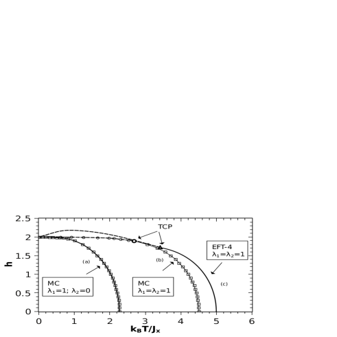
We obtained the phase diagrams in the $h-k_{B}T/J_{x}$ plane for $\lambda_{1}=\lambda_{2}=1$ of the model 1 by using EFT-4 and MC simulatons. Both methods confirmed the existence of a tricritical point in a critical frontier separating the SAF order with the paramagnetic disorder as shown in Figure 2. For completeness, Figure 2 also includes the critical frontier obtained by MC simulatons for the particular case $\lambda_{1}=1$, $\lambda_{2}=0$ (square lattice), which lacks of first-order criticality viana2009 . In what effective-field calculations concerns, we obtain the critical frontier, which consists of the transition temperature as a function of the external magnetic field, separating the SAF and P phases, by simultaneously solving the three transcendental equations Eqs. (16), (17) and (18). The range of ratio $h=H/J_{x}$ determines the limits of second-order $(0<h<h_{t})$ and first-order $(h_{t}<h\leqslant 2)$ phase-transition frontiers, where $(h_{t},k_{B}/J_{x}T_{t})$ is the tricritical point (TCP). From Landau theory, the TCP is calculated by the condition given by $A_{1}(m,T_{t},H_{t})=1$, $A_{3}(m,T_{t},H_{t})=0$ and $A_{5}(m,T_{t},H_{t})>0$, obtaining in EFT-4 the following values: $h_{t}=1.72$ and $k_{B}T_{t}/J_{x}=3.42$. The temperature variation of $m_{s}(T,H)$ for fixed reduced field $H/J_{x}$ present two type of behavior. The first for low-field the order parameter decrease to zero continuously as the reduced temperature approaches to the critical point, the temperature ($H$ fixed) where $m_{s}=0$ is the second-order phase transition temperatute, $T_{c}(H)$. On the other hand, when we are at high-fied the temperature at which the order parameter make a jump discontinuity is the first-order phase transitions going to zero discontinuously at the point $T_{c}^{∗}(H)$. For h value greater than the upper limit of these field (i. e., $h>h_{c}=2.0$), the system exhibits no phase transition (the order parameter is null for all finite temperature, $T>0$)

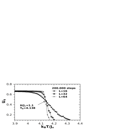
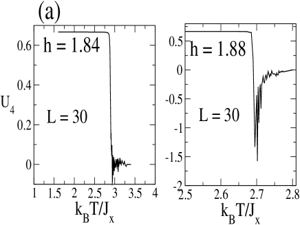
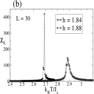
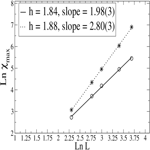
In order to obtain relevant critical points to get the critical frontier in MC simulations, we estimate the critical temperature for a given value of field by a finite-size scaling analysis. For instance, for $h=H/J_{x}=1.1$, Figure 3 shows how the critical temperature was located around the crossing point of $U_{4}-k_{B}T/J_{x}$ curves for sizes $L=16,32,64$, resulting in $k_{B}T_{c}/J_{x}\sim 4.14$. Note that critical temperatures for lower fields are superestimated by the EFT-4 technique (see Figure 2). The limit of the second-order frontier was found by obtaining several $U_{4}-k_{B}T/J_{x}$ curves for different field values for a given lattice size. Consequently, we found the beginning of the first-order criticality after detecting a change in the behavior of the Binder Cumulant curve above a certain value of field. This is well exemplified in Figure 4, for two different field values $h=1.84$, $1.88$, for $L=30$. Figure 4a shows that the Binder Cumulant curve already presents a clear first-order transition for $h=1.88$, because of the sharply negative fluctuated peaks around the pseudocritical temperature. Moreover, Figure 4b also suggests this first-order criticality by the aparent Delta-Dirac form of the susceptivility, for $h=1.88$. In order to confirm what is suggested in short lattice sizes, we draw upon the fact that around the critical temperature of a phase transition the susceptibility peaks behave as $\chi_{max}\sim L^{\theta}$, where $\theta=d$ ($d$ is the lattice dimension), for a first-order criticality, whereas $\theta=\gamma/\nu$ for a second-order one. Consequently, Figure 5 shows a finite-size scaling of the susceptibility peak versus $L$, for sizes $L=15$, $20$, $30$ and $40$. For $h=1.84$, we estimated $\theta=1.98(3)$, which is (within the error bar) an universal value gupta ; flandau for the second-order criticality of the three-dimensional Ising model. For $h=1.88$, $\theta\sim 2.8$, which is close to $d=3$, which suggests a first-order transition. Therefore, the tricritical point must be in the interval $1.84<h<1.88$. On the other hand, the first-order curve must end at $h_{c}=2$.

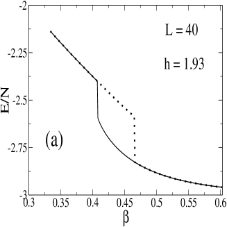
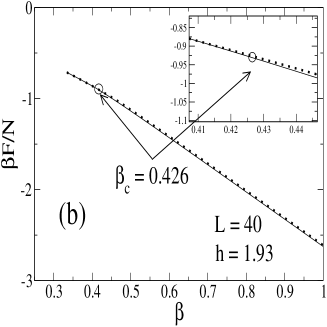
We could estimate some points of the first-order frontier by a finite-size scaling method, however, in order to avoid finite-size problems to obtain well behavied curves for the specific heat or the susceptibility around critical points belonging to the first-order frontier, we decided to estimate the corresponding critical temperatures for given fields by computing the free energy versus $\beta=1/k_{B}T$, from Monte Carlo data of energy versus $\beta$, for a given size. For instance, in figure 6a it is shown the hysteresis effect from energy data around the critical temperature obtained when cooling or heating the system too fast. This is because of huge intrinsic autocorrelation times in finite-size systems. We can improve the location of the critical temperature by obtaining the associated free energies of the low- and high-temperature branchescomputersim . Consequently, the crossing point of the free energy branches gives a good estimation of the critical temperature, inasmuch the stable phase has the lower free energy, as shown in figure 4b.

The first-order frontier in MC simulations does not present a reentrant behavior as EFT-4 frontier does. So, this reentrance seems to be an artifact of the effective-field approach.

IV Conclusions

In summary, we investigated the anisotropic three-dimensional nearest-neighbor Ising model with competitive interations in an uniform longitudinal field. We obtained the phase diagram in the plane $h-k_{B}T/J_{x}$, where the critical frontier separates the SAF order with the paramagnetic disorder. For lower fields, the EFT-4 approach superestimates the critical temperatures obtained by MC simulations. A tricritical point was found for $1.84<h<1.88$, by a finite-size analysis. At low temperatures EFT-4 calculations show a reentrant first-order frontier, which does not appear by MC simulations. It suggests that improvements in treating correlations, or by increasing the cluster size in the Effective-Field approach, could correct this reentrant curve. At zero temperature, the critical field is exactly obtained, so $h_{c}=2.0$. Our quantitative estimation for the tricritical point could be bettered by using larger lattice sizes with better Metropolis Monte Carlo techniques like Parallel Tempering.

ACKNOWLEDGEMENT

We thank Professor David P. Landau for fruitful suggestions in the VI BMSP (Brazilian Meeting on Simulational Physics 2011). This work was partially supported by CNPq (Edital Universal) and FAPEAM (Programa Primeiros Projetos - PPP) (Brazilian Research Agencies).

References

- (1) L. J. de Jongh et al., Physica 58, 277(1972) .
- (2) L. J. de Jongh et al., J. Appl. Phys. 40, 1363(1969).
- (3) P. Bloembergen et al., Proc. Int. Conf. Magn., Grenoble 1970 J. Phys., suppl. no. 2-3 Tome 32, 879(1971).
- (4) L. J. de Jongh et al., Proc. Int. Conf. Magn., Grenoble 1970 J. Phys., suppl. no. 2-3 Tome 32, 880(1971).
- (5) A. R. Miedema, Proc. Int. Conf. Magn., Grenoble 1970 J. Phys., suppl. no. 2-3 Tome 32, 305(1971).
- (6) C. A. M. Mulder et al., Physica B+C 113, 380(1982).
- (7) G. Heger et al., Solid State Commun. 12, 1157(1973).
- (8) See, e.g., C. Domb, in Phase Transitions and Critical Phenomena, edited by C. Domb and M. S. Green (Academic, New York, 1974), Vol. 3.
- (9) W. P. Wolf, J. Phys. (Paris) Suppl. 32, C1(1971).
- (10) T. Graim and D. P. Landau, Phys. Rev. B 24, 5156(1981). Phys. Rev. Lett. 68, 9(1992).
- (11) W. Stout and R. C. Chisholm, J. Chem. Phys. 3C, 979(1962).
- (12) D. Hone, P. A. Montano and T. T. Tonegawa Phys. Rev. B 12, 5141(1975).
- (13) H. Sato, J. Phys. Chem. Solids 19, 74(1961).
- (14) C. G. B. Garrett, J. Chem. Phys. 19, 1154(1951).
- (15) J. M. Ziman, Proc. Phys. Soc., London, Sect. A 64, 1108(1951).
- (16) M. Zukovic, A. Bobak and T. Idogaki J. Magn. Magn. Mater. 192, 363(1999).
- (17) P. A. Slotte, J. Phys. C 16, 2935(1983).
- (18) Minos A. Neto and J. Ricardo de Sousa, Phys. Rev. B 70, 224436(2004).
- (19) D. P. Landau, Phys. Rev. B 16, 4164(1977).
- (20) D. P. Landau, Phys. Rev. B 14, 255(1976).
- (21) For simple cubic lattice, see A. M. Ferrenberg and D. P. Landau, Phys. Rev. B 44, 5081(1991).
- (22) A. Bienenstock and J. Lewis, Phys. Rev. 160, 393(1967).
- (23) J. Roberto Viana, Minos A. Neto and J. Ricardo de Sousa Phys. Latt. A 373, 2413(2009).
- (24) M. Metropolis et al., J. Chem. Phys. 21, 1087(1953); R. J. Glauber, J. Math. Phys. 4, 294(1963).
- (25) K. Hukushima, and K. Nemoto J. Phys. Jpn. 65, 1604(1996).
- (26) U. Wolff, Phys. Rev. Lett. 62, 361(1989); R. H. Swendsen, and J. S. Wang, Phys. Rev. Lett. 58, 86(1987).
- (27) B. A. Berg, and T. Neuhaus, Phys. Lett. B 267, 249(1991); Phys. Rev. Lett. 68, 9(1992).
- (28) F. Wang, and D. P. Landau, Phys. Rev. Lett. 86, 2050(2001).
- (29) L. Onsager, Phys. Rev. 65, 117(1944).
- (30) M. E. Fisher, in Proceedings of the International Summer School Enrico Fermi, Course 51, Varenna 1970, edited by M. S. Green (Academic, New York, 1971).
- (31) K. Binder, Z. Phys. B: Condens. Matter 43, 119(1981).
- (32) Denise A. do Nascimento et al., J. Magn. Magn. Mater. 324, 2429(2012).
- (33) R. Honmura and T. Kaneyoshi, J. Phys. C 12, 3979(1979).
- (34) R. Gupta and P. Tamayo, IJMPC 7 , 305(1996).
- (35) Alan M. Ferrenberg and D. P. Landau, Phys. Rev. B 44, 5081(1991).
- (36) see pages 111-116 of W. Janke, Computer Simulations of Surfaces and Interfaces, edited by B. Dunweg, D. P. Landau, A. I. Milchev (NATO Science Series 2002).