Estimating Nuisance Parameters in Inverse Problems
Abstract
Many inverse problems include nuisance parameters which, while not of direct interest, are required to recover primary parameters. Structure present in these problems allows efficient optimization strategies — a well known example is variable projection, where nonlinear least squares problems which are linear in some parameters can be very efficiently optimized. In this paper, we extend the idea of projecting out a subset over the variables to a broad class of maximum likelihood (ML) and maximum a posteriori likelihood (MAP) problems with nuisance parameters, such as variance or degrees of freedom. As a result, we are able to incorporate nuisance parameter estimation into large-scale constrained and unconstrained inverse problem formulations. We apply the approach to a variety of problems, including estimation of unknown variance parameters in the Gaussian model, degree of freedom (d.o.f.) parameter estimation in the context of robust inverse problems, automatic calibration, and optimal experimental design. Using numerical examples, we demonstrate improvement in recovery of primary parameters for several large-scale inverse problems. The proposed approach is compatible with a wide variety of algorithms and formulations, and its implementation requires only minor modifications to existing algorithms.
1 Introduction
Many inverse problems can be formulated as optimization problems of the form
| (1) |
where is a twice differentiable function, , is a primary set of parameters of interest, while is a secondary set of nuisance parameters, such as variance parameters, application-specific tuning parameters, regularization parameters, or degrees of freedom parameters. In many settings, .
A rich source of examples in (1) is the class of separable least-squares problems, extensively studied over the last 40 years [11, 10, 15]. A problem in this class is given by
| (2) |
where the matrix is parametrized by . Note that has a very special form in this case, and . For problems in this class, the major insight is to exploit the structure of the problem to obtain a reduced problem
| (3) |
where
| (4) |
At first glance, this does not make the problem easier to solve. However, it turns out that (3) can be solved using black-box approaches as long as we re-evaluate for any given , but treat as fixed whenever is updated. The problem (4) has a closed form solution, and as noted in [10], this approach converges much faster than optimization approaches to minimize the full functional (2) using descent methods for .
In this paper, we consider problems of type (1), where we can easily compute . We show that many algorithms for solving instances of (1) with fixed can be easily modified to solve the joint inverse problem in and . We provide explicit details for several important classes of problems in (1), including variance and degrees of freedom (d.o.f.) estimation, and automatic calibration of nonlinear least squares and robust inverse problem formulations.
The paper proceeds as follows. In Section 2, we review the necessary theory underlying our approach to the entire class (1). In Section (3), we discuss the role of nuisance parameters, such as variance and degrees of freedom, in MAP estimation formulations. We present two important applications in detail:
-
1.
Variance estimation in multiple data sets (see [5]).
-
2.
Estimation of variance and d.o.f. for Student’s t formulations (see [13]).
Both are illustrated on a seismic imaging problem where the data are contaminated with various types of noise.
In Section 4, we discuss the automatic calibration problem, where the forward model includes a calibration parameter that needs to be estimated. We illustrate the approach on a seismic imaging problem where the calibration parameter are frequency-dependent source-weights. We discuss the application of the proposed approach to Optimal Experimental Design in section 5.
Finally, we discuss other possible applications and present conclusions.
2 General Formulation
We consider problems of the form (1), and assume that for any given , one can easily find
| (5) |
This condition can be relaxed, and can be considered a local minimum. Rather than working to solve (1), we can instead focus on the reduced objective
| (6) |
This approach is justified by the following theorem, adapted from [4, Theorem 2].
Theorem 2.1
Suppose that and are open, and is twice continuously differentiable on . Define the optimal value function
| (7) |
Suppose that and are such that and is positive definite. Then there exist neighbourhoods of and and a twice continuously differentiable function where is the unique minimizer of on .
Then is twice continuously differentiable, with
| (8) | |||||
| (9) |
Remark 2.2
Theorem 8 provides sufficient conditions for existence of the first and second derivatives of . In practice, these derivatives may exist even if the smoothness hypotheses are not satisfied. Consider . In this case, , so is smooth even though is not.
Theorem 8 suggests a natural approach to designing algorithms for minimizing . In the unconstrained case (i.e. is the whole space), consider iterative methods of the form
| (10) |
Specifically, yields Cauchy’s steepest descent, yields a modified Newton method, and approximations to that use only first order derivative information yield Gauss-Newton or Levenberg-Marquardt type methods. A quasi-Newton method such as BFGS or L-BFGS may be similarly implemented using only information from (8).
If is a closed and bounded set that allows a simple projection, such as a set of box constraints (, an ellipsoidal set , or the -norm ball (), this can be exploited to solve (1). For example, we can use a modified projected gradient method
| (11) |
or an appropriately modified projected quasi-Newton method, such as the one described in [18]. The point is that the structure of does not enter into the computation of (8) or (9), so a natural strategy is to compute these quantities first and then apply methods that exploit the structure of . Moreover, we show in the next corollary that the point satisfies the first order necessary conditions for the original (constrained) problem.
Corollary 2.3
Suppose the hypotheses of Theorem 8 hold, and the additional constraint is imposed, where is a closed convex set. If satisfies the first order necessary conditions for , then with satisfies the first order necessary conditions for .
Proof:
The first order necessary conditions for (1) are
| (12) |
where is the normal cone to at the point (see [17] for details). The first order necessary condition for to be a minimizer of the reduced objective (6) is
| (13) |
Since we have by Theorem 8, satisfies (12) if and only if satisfies (13). On the other hand, satisfies the first equation of (12) by construction.
Thus, for many applications (both constrained and unconstrained), we can systematically extend many standard algorithms for minimizing with fixed to extended problems (1). This approach avoids computing the full Hessian of the modified objective (9), since it involves .
In the next sections, we present some of these applications and provide full algorithmic details and numerical work.
3 Complicating Parameters in Maximum Likelihood Estimation
Many inverse problems can be formulated as maximum likelihood (ML) problems within a statistical modeling framework. Given data , we want to solve for parameters of interest , using the fact that the parameters are related to the data via a (possibly nonlinear) forward model:
| (14) |
The term in (14) reflects a statistical model of the discrepancy between the model and the true data . Independent, identically distributed (i.i.d.) Gaussian errors are a common choice, and even though the variance parameter is unknown, it does not affect the maximum likelihood formulation in . This is not true if the data come from different sources, with each group having its own parameter .
More generally, may come from a range of parametric distributions. The Student’s t distribution has been applied in many instances where large measurement errors are common or unexplained artifacts in the data are an issue [1, 2, 13]. These applications require estimates for degrees of freedom and variance parameters even with the i.i.d. assumption on the errors.
If we take to be unknown nuisance parameters, the general maximum likelihood formulation for estimating in model (14) takes the form (1). The method proposed in this paper is well suited for online estimation of , and in the remainder of the section we provide full exposition for the multiple sources of error example and for Student’s t hyperparameter estimation.
3.1 Variances in Multiple Data Sets
Estimating variance parameters in multiple datasets is an important problem in many areas, including drug and tracer kinetics [5], and geophysics. In this section, we review the formulation presented in [5], and show that the algorithm derived in [5] follows immediately from the general approach we propose here, i.e. it is a Gauss-Newton method of form (10). We present a numerical example, illustrating the importance of variance parameter estimation for a large-scale geophysical inverse problem. We also extend the approach to the (fully observed) multivariate Gaussian case with correlations between measurement errors.
We are given experiments indexed by , each of which yields measurements and has its own variance parameter . All experiments share a common set of primary parameters :
| (15) |
where , is the modeling operator for the experiment and . If the variance parameters are fixed, the ML estimation problem for is given by
| (16) |
The joint ML estimation problem for and is given by
| (17) |
This is a special example of (1).
With fixed, (17) separates, and (5) has a closed form solution, which we find by taking the gradient with respect to each and setting it to :
| (18) |
This quantity is precisely the population variance estimate. The modified problem (6) is now given by
| (19) |
The gradient of this objective is given by
| (20) |
while the Gauss-Newton (GN) Hessian approximation is given by
Note that this is an approximation to , and completely ignores the term in (9). The term can actually be explicitly calculated for this application, and turns out to be a dense negative definite correction to the Hessian approximation. If we ignore it, we recover the algorithm in [5], which can be seen by forming the GN subproblem:
| (21) |
This expression matches [5, (12)] up to a constant. However, while in [5] the function (21) came about as a cleverly constructed proxy objective for (17), we can now view it as a natural GN approximation to the modified objective (19).
Example: Full Waveform Inversion
Full waveform inversion (FWI) is an approach to obtain gridded subsurface velocity parameters from seismic data. Experiments are conducted by placing explosive sources on the surface and recording the reflected waves with an array of receivers on the surface. FWI is naturally cast as a nonlinear least squares optimization problem [19, 16], and fits in the framework described above. The data, , in this case represents the Fourier transform of the recorded time series for frequency . The corresponding modeling operator, , inverts a discretized Helmholtz operator for the frequency and the gridded velocity field and samples the wavefield at the receiver locations. Here, denotes the sampling operator and each column of the matrix is a gridded source function.
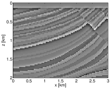
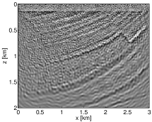
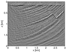
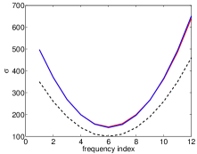
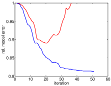
To illustrate the approach we use a subset of the well-known Marmousi benchmark model, depicted in figure 1 (a). The model is discretized on a 201 301 grid with 10 m grid spacing. We generate data for 151 sources, 301 receivers (i.e., )—all equi-spaced and located at the surface— and frequencies between 3 and 25 Hz. Typically, the data has a lower signal to noise ratio for the low and high frequencies. To emulate this situation we add Gaussian noise to the measurements with variance . We use an L-BFGS method to solve both the the modified optimization problem (19) and the original problem for a fixed for all . The results after 50 iterations are shown in figure 1(b,c). The corresponding error between the reconstructed and true model is shown in figure 1(d). Finally, we show the estimated variance at the final model for both reconstructions in figure 1(e). The reconstruction obtained by solving the modified problem is clearly better. Interestingly enough, the variance estimates for both models are almost identical.
3.2 Correlated Multivariate Observations
The results from the previous case can be generalized to general variance estimation in a multivariate inverse problem setting with correlated errors. Consider the model (15), where now we take . In this case, all of the are in of the same dimension. The ML objective corresponding to (17) is given by
| (22) |
The point here is that despite the generalization to full , we still have a closed form solution analogous to (18):
| (23) |
This can be shown by a simple derivative computation:
Therefore, the variable projection method applies immediately to (22), at the cost of computing, at each iteration in , the standard multivariate variance estimate (23). If this cost is high (i.e. if each has high dimension), there are still a number of strategies that make the proposal feasible. For example, (23) can be computed approximately using a random subset of the residuals.
In addition to improving the primary parameters, incorporating nuisance parameter estimation can be helpful to post-processing analysis such as uncertainty quantification. For example, the estimate of at the final solution can be used to estimate the posteriori covariance matrix in the model space [9].
3.3 Degrees of Freedom and Variance Estimation for Student’s t Formulation
Many applications require robust formulations to obtain reasonable results with noisy data or in cases where a portion of the data is unexplained by the forward model (e.g. in the presence of coherent artifacts). A useful way to derive these formulations is to begin with the statistical model (15) where the noise term is modelled using a particular parametric density, and then formulate the maximum a posteriori (MAP) likelihood problem. The least-squares formulation corresponds to a Gaussian assumption on (see section 3.1), while assuming a Laplacian distribution leads to a one-norm penalty on the data-misfit.
As shown by [2, Theorem 2.1], in cases where unexplained artifacts may be large or constitute a significant portion of the data, it is better to use heavy-tailed densities. A prime example is the Student’s t, whose density is given by
| (24) |
This density was first successfully used in [13] in the data fitting context. The degrees of freedom parameter was seen as a tuning parameter, smoothly transitioning between heavy-tailed and near-Gaussian behaviour; and were fit using Expectation Maximization (EM) and scoring methods. This density was also successfully used in the Kalman smoothing context [8], where it was suggested that the EM algorithm can be used to fit meta-parameters. Recent work using the Student’s t distribution [2, 3, 1] has side-stepped the problem, using fixed values for and .
In this section, we show that the general projection approach can be used to solve the joint inverse problem, treating scale and degrees of freedom as nuisance parameters. We propose a novel simple method, different from EM or scoring methods discussed in [13], for estimating scale and degrees of freedom for any given set of residuals. Given the model (15), the full MAP Student’s t estimation problem is given by
| (25) |
where . Following the philosophy presented in the paper, we solve the problem by defining the modified objective
| (26) |
with
The two-dimensional optimization problem in required to evaluate can be solved using a customized routine or a black-box optimization code. An application is presented below.
Example: Traveltime tomography:
We consider a cross-well traveltime tomography problem. In this case, sources and receivers are placed in vertical wells and the data consists of picked traveltime of first arrivals. Since the data are typically very noisy, a portion of the traveltimes may be picked erroneously, motivating the use of robust penalties for the inversion. The traveltimes are computed by a geometric optics approach, where wave propagation is modeled via rays. The traveltime between a given source and receiver is simply the integral of the reciprocal velocity along the corresponding ray-path. By assuming small perturbations of a known background velocity, we arrive at a linear modeling operator with a fixed ray geometry. The data are the traveltime perturbations, while the primary parameter of interest is the velocity perturbation, both taken with respect to a known background model.
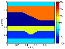
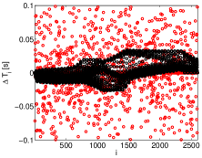
In this example, we consider a constant background velocity, so that the ray paths are straight lines. The modeling operator is therefore essentially a Radon transform, which is often used in medical X-ray imaging applications. The true velocity perturbation is discretized on a 51 51 grid and is shown in figure 2(a). The corresponding data for 51 sources and receivers and the added outliers are shown in figure 2(b). We regularize the inversion by inverting for the primary parameters on a courser grid of size 26 26. We then interpolate back to the fine grid using 2D cubic interpolation. The modified optimization problem is now given by
| (27) |
where are the measured traveltime perturbations, is the velocity perturbation, is the modeling operator which combines the Radon transform and interpolation, and is obtained by solving (26) using a Nelder-Mead method [14].
Note that we may treat as fixed when designing an algorithm to solve (27), as long as the parameters are re-estimated at every evaluation of and its derivatives. To solve (27) we use a modified Gauss-Newton algorithm which calculates the updates by solving
| (28) |
where and is a positive approximation of the Hessian . We solve the subproblems using CG. Note that when , the algorithm converges in one GN iteration, which is computed by applying CG to the normal equations.
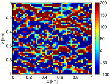
We compare the following three approaches: i) least-squares, shown in figure 3(a), ii) Student’s t with a fixed wich is estimated once at the initial residual, shown in figure 3(b), and iii) Student’s t where we estimate at each iteration, shown in figure 3(c). In order to understand the difference between the latter two cases, we show histograms of the initial and final residuals as well as the influence function for the corresponding in figures 4(a-c). Clearly, re-fitting the at each iteration allows the inversion to home in on the good data while ignoring the outliers.
4 Automatic calibration
In this section we consider the case where the forward model includes a calibration factor :
| (29) |
In case of the non-linear data-fitting problem described earlier, the modified objective is given by
| (30) |
where
| (31) |
The motivating example that led us to consider this class of problems is presented below.
Example: FWI with source estimation:
Seismic data can be interpreted as the Green’s function of the subsurface, parametrized by , convolved with an unknown (bandlimited) source signature. In the frequency-domain we can model the uknown source signature by multiplication with a complex scalar for each frequency. The problem of interest is now formulated as
| (32) |
where the index runs over frequency. Just as in the variance parameter case, the parameters are linked only through the parameters , and for a given the problem decouples completely, giving
| (33) |
We consider the least-squares and Student’s t penalty, and use a scalar Netwon-type method to solve (33):
| (34) |
where , is the gradient of the penalty function and is (a positive definite approximation of) the Hessian . In particular, we have:
-
•
least-squares: , and .
-
•
Student’s t: , and .
For more details on the Student’s t approach we refer to [2].
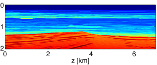
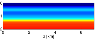
We generate seismic data for the velocity model depicted in figure 5 (a) with a time-domain finite difference code. The data consists of 141 sources and 281 receivers and has a recording time of 4 seconds. 10 percent of the data is corrupted with large outliers.
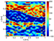
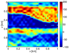
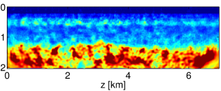
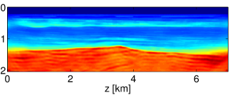
We invert the data in several stages, moving from low to high frequencies. Each stage uses only a few frequencies and the output is used as initial guess for the subsequent stage. This is a well-known strategy in FWI to avoid local minima [6]. We use an L-BFGS method to solve the resulting optimization problems, starting from the initial model shown in figure 5 (b). The results are shown in figure 5 (c,d). The Student’s t approach recovers the most important features of the model whereas the least-squares approach leads to a very noisy model.
5 Optimal experimental design
In Optimal Experimental Design one is concerned with finding optimal design parameters for which a set of test models can be recovered from the corresponding simulated data . This can be formulated as an optimization problem (cf. [12] and references cited therein)
| (35) |
Here, measures the quality of the reconstruction (lower is better) and measures the cost of a given experimental parameter setting. Note that (35) is actually the reduced problem for the joint optimization problem
| (36) |
where has been projected out.
The downside to this approach is that projecting out is expensive, since every iteration of any algorithm to find requires repeated evaluations of , for each model in the class . Rather than projecting out , we can project out the design parameter to arrive at a different reduced objective
| (37) |
where . In many cases, can be computed cheaply without re-evaluating the whole forward model. The forward modeling need only be done when is updated, as in the other applications that we presented. For example, may represent a vector of source weights for waveform inversion in which case (see section 3.1). Since the data are linear in the source, we need only invert the Helmholtz system once (for a given ), and therefore can be computed relatively cheaply. A reasonable penalty on might be the one-norm, in which case we are looking for a setup with as few sources as possible. Alternatively, we can impose a two-norm penalty on to find a setup where the sources require the least amount of energy.
6 Discussion and Conclusions
Many inverse problems involve nuisance parameters that are not of primary interest but can have significant influence on the estimation of primary parameters. Common examples include variance, degree of freedom, and calibration parameters. These issues arise in a great variety of applications, including pharmacokinetic modeling [5], seismic inverse problems [19], dynamic systems [7], uncertainty quantification [9] and optimal experimental design [12].
In this paper, we proposed a straightforward approach to fitting these nuisance parameters on the fly, while solving the overall inverse problem. Specifically, we formulated the problem as a joint optimization over primary parameters and nuisance parameters (1), and showed that for a large class of problems, one can simply project out the parameters by solving (5). In this least squares case, this idea has been carefully studied under the name variable projection [15, 10]. As we showed, these ideas extend nicely to the entire class (1). In particular, Theorem 2.1 and Corollary 2.3 characterize the general approach and are the basis for algorithm design of first and second order methods.
An immediate consequence of the work is the ability to modify first and second order algorithms
that exploit particular application structure to also fit nuisance parameters. We
demonstrated this in practice using several (large scale) inverse problems:
| Application | Complicating parameters | Algorithm |
|---|---|---|
| full waveform inversion | variances in multiple datasets | L-BFGS |
| travel time tomography | student’s t parameters | Gauss-Newton with CG |
| automatic calibration | unknown source amplitudes | L-BFGS |
In the case of variances in multiple datasets, the proposed approach matches the algorithm proposed in [5], and therefore the development we presented provides an alternative (and significantly simpler) derivation. We have also shown that the approach can be easily extended to estimate covariances between error sources in the case where we have multivariate observations in Section 3.2.
In the case of student’s t parameters, it is interesting to note that when estimating degrees of freedom for fixed residuals, our approach matches the one used in the MASS library of the R programming language [20]. To our knowledge, this approach has not been used for fitting degrees of freedom in general inverse problems, and in fact Lange, Little, and Taylor [13], who first proposed Student’s t inversion, advocated a very different (EM-type) approach for degrees of freedom fitting.
From a theoretical point of view, the method we propose can be used to solve a variety of inverse problems from the general class (1). From a practical point of view, the main selling point of the proposed approach is the ability to modify existing methods to solve for nuisance parameters on the fly.
7 Acknowledgements
This work was in part financially supported by the Natural Sciences and Engineering Research Council of Canada Discovery Grant (22R81254) and the Collaborative Research and Development Grant DNOISE II (375142-08). This research was carried out as part of the SINBAD II project with support from sponsors of the SINDBAD consortium.
References
- [1] A.Y. Aravkin, J.V. Burke, and G. Pillonetto. Robust and trend-following student’s t kalman smoothers. Optimization Online Preprint, 2012.
- [2] A.Y. Aravkin, M.P. Friedlander, F.J. Herrmann, and T. van Leeuwen. Robust inversion, dimensionality reduction, randomized sampling. Submitted to Math. Prog., November 2011.
- [3] A.Y. Aravkin, M. Styer, Z. Moratto, A. Nefian, and M. Broxton. Student’s T Robust Bundle Adjustment Algorithm, November 2011. http://arxiv.org/abs/1111.1400.
- [4] Bradley M. Bell and James V. Burke. Algorithmic differentiation of implicit functions and optimal values. In Christian H. Bischof, H. Martin Bücker, Paul D. Hovland, Uwe Naumann, and J. Utke, editors, Advances in Automatic Differentiation, pages 67–77. Springer, 2008.
- [5] Bradley M. Bell, James V. Burke, and Alan Schumitzky. A relative weighting method for estimating parameters and variances in multiple data sets. Computational Statistics & Data Analysis, 22(2):119–135, July 1996.
- [6] Carey Bunks, Fatimetou M. Saleck, S. Zaleski, and G. Chavent. Multiscale seismic waveform inversion. Geophysics, 60(5):1457–1473, 1995.
- [7] L. Fahrmeir and G. Tutz. Multivariate Statistical Modelling Based on Generalized Linear Models. Springer Series in Statistics. Springer, 2010.
- [8] Ludwig Fahrmeir, Rita Kunstler, and Seminar Fur Statistik. Penalized likelihood smoothing in robust state space models. Metrika, 49:173–191, 1998.
- [9] H. P. Flath, L. C. Wilcox, V. Akçelik, J. Hill, B. van Bloemen Waanders, and O. Ghattas. Fast algorithms for bayesian uncertainty quantification in large-scale linear inverse problems based on low-rank partial hessian approximations. SIAM J. Sci. Comput., 33(1):407–432, February 2011.
- [10] Gene Golub and Victor Pereyra. Separable nonlinear least squares: the variable projection method and its applications. Inverse Problems, 19(2):R1, 2003.
- [11] G.H. Golub and V. Pereyra. The differentiation of pseudo-inverses and nonlinear least squares which variables separate. SIAM J. Numer. Anal., 10(2):413–432, 1973.
- [12] L. Horesh, E. Haber, and L. Tenorio. Optimal experimental design for the large-scale nonlinear ill-posed problem of impedance imaging. In large-scale inverse problems and quantification of uncertainty, Wiley series in computational statistics, pages 273–290. Wiley, 2011.
- [13] Kenneth L. Lange, Roderick J. A. Little, and Jeremy M.G. Taylor. Robust statistical modeling using the t distribution. Journal of the American Statistical Association, 84:881–896, 1989.
- [14] J. A. Nelder and R. Mead. A simplex method for function minimization. Computer Journal, 7:308–313, 1965.
- [15] M. R. Osborne. Separable least squares, variable projection, and the Gauss-Newton algorithm. Electronic Transactions on Numerical Analysis, 28(2):1–15, 2007.
- [16] R G Pratt, C Shin, and Gj Hicks. Gauss-newton and full newton methods in frequency-space seismic waveform inversion. Geophysical Journal International, 133(2):341Ã362, 1998.
- [17] R.T. Rockafellar. Convex Analysis. Priceton Landmarks in Mathematics. Princeton University Press, 1970.
- [18] Mark Schmidt, Ewout Van Den Berg, Michael P. Friedlander, and Kevin Murphy. Optimizing costly functions with simple constraints: A limited-memory projected quasi-newton algorithm. In Proc. of Conf. on Artificial Intelligence and Statistics, pages 456–463, 2009.
- [19] Albert Tarantola. Inversion of seismic reflection data in the acoustic approximation. Geophysics, 49(8):1259–1266, 1984.
- [20] W. N. Venables and B. D. Ripley. Modern Applied Statistics with S. Springer, New York, fourth edition, 2002. ISBN 0-387-95457-0.
 |
 |
 |
| (a) | (b) | (c) |
 |
 |
| (d) | (e) |
 |
 |
| (a) | (b) |
 |
 |
 |
| (a) | (b) | (c) |
| (a) | (b) | (c) |
 |
 |
| (a) | (b) |
 |
 |
| (c) | (d) |