A Permutation Approach to Testing Interactions in Many Dimensions

Noah Simon Department of Statistics, Stanford University, nsimon@stanford.edu Rob Tibshirani Department of Statistics, Stanford University, Department of Health Research and Policy, Stanford University
Abstract

To date, testing interactions in high dimensions has been a challenging task. Existing methods often have issues with sensitivity to modeling assumptions and heavily asymptotic nominal p-values. To help alleviate these issues, we propose a permutation-based method for testing marginal interactions with a binary response. Our method searches for pairwise correlations which differ between classes. In this manuscript, we compare our method on real and simulated data to the standard approach of running many pairwise logistic models. On simulated data our method finds more significant interactions at a lower false discovery rate (especially in the presence of main effects). On real genomic data, although there is no gold standard, our method finds apparent signal and tells a believable story, while logistic regression does not. We also give asymptotic consistency results under not too restrictive assumptions.

Keywords: correlation, high dimensional, logistic regression, false discovery rate

1 Introduction

In many areas of modern science, massive amounts of data are generated. In the biomedical sciences, examples arise in genomics, proteomics, and flow cytometry. New high-throughput experiments allow researchers to look at the dynamics of very rich systems. With these vast increases in data accumulation, scientists have found classical statistical techniques in need of improvement, and classical notions of error control (type 1 error) overwhelmed.

Consider the following two class situation: our data consists of n𝑛n observations, each observation with a known class label of 1 or 2, with p𝑝p covariates measured per observation. Let y𝑦y denote the n𝑛n-vector corresponding to class (with n1subscript𝑛1n_{1} observations in class 111 and n2subscript𝑛2n_{2} in class 222), and X𝑋X, the n×p𝑛𝑝n\times p matrix of covariates. We often assume each row of X𝑋X is independently normally distributed with some class specific mean μy(i)psubscript𝜇𝑦𝑖superscript𝑝\mu_{y(i)}\in\mathbb{R}^{p} and covariance Σy(i)subscriptΣ𝑦𝑖\Sigma_{y(i)} (for instance in quadratic discriminant analysis). Here, we are interested in differences between classes. A common example is gene expression data on healthy and diseased patients: the covariates are the genes (p20,000similar-to𝑝20000p\sim 20,000), the observations are patients (n100similar-to𝑛100n\sim 100) belonging to either the healthy or diseased class. Here, one might look at differences between classes to develop a genetic prognostic test of the disease, or to better understand its underlying biology. Recent high dimensional procedures have focused on detecting differences between μ1subscript𝜇1\mu_{1} and μ2subscript𝜇2\mu_{2} by considering them one covariate at a time.

In this paper we consider the more difficult problem of testing marginal interactions. In a fashion similar to the approaches used in large scale testing of main effects (see e.g Dudoit et al. (2003), Tusher et al. (2001) and Efron (2010)), we do this on a pair by pair basis.

The standard approach for this problem has been to run many bivariate logistic regressions and then conduct a post-hoc analysis on the nominal p-values. Buzkova et al. (2011) has a nice summary of the subtle issues that arise in testing for just a single interaction in a regression framework. In particular, a permutation approach cannot be simply applied because it tests the null hypothesis of both no interaction and no main effects at the same time. In the high-dimensional setting with FDR estimates, these issues are compounded.

The logistic regression based methods are all derived from what we call a forward model, that is, a model for the conditional distribution of Y|Xconditional𝑌𝑋Y|X. In contrast, a backward model (discussed below) is a model for the conditional distribution of X|Yconditional𝑋𝑌X|Y. We propose a method, based on a backwards model, to approach this same problem. By using this backwards framework we avoid many of the pitfalls of standard approaches: we have a less model-based method, we attack a potentially more scientifically interesting quantity, and we can use a permutation null for FDR estimates. Our approach is unfortunately only for binary response — the backwards model is more difficult to work with for continuous y𝑦y.

In this paper we develop our method, and show its efficacy as compared to straightforward logistic regression on real and simulated data. We explain how to deal with nuisance variables, and give insight into our permutation-based estimates of FDR. We also give some asymptotic consistency results.

2 Existing Methods

We begin by going more in-depth on the standard approach and its issues. In general one might like to specify a generative logistic model for the data (a forward model) of the form

logit[P(yi=1|Xi,)]=β0+j=1pβjXi,j+k<jγj,kXi,jXi,klogitPsubscript𝑦𝑖conditional1subscript𝑋𝑖subscript𝛽0superscriptsubscript𝑗1𝑝subscript𝛽𝑗subscript𝑋𝑖𝑗subscript𝑘𝑗subscript𝛾𝑗𝑘subscript𝑋𝑖𝑗subscript𝑋𝑖𝑘\operatorname{logit}\left[\operatorname{P}(y_{i}=1|X_{i,\cdot})\right]=\beta_{0}+\sum_{j=1}^{p}\beta_{j}X_{i,j}+\sum_{k<j}\gamma_{j,k}X_{i,j}X_{i,k} (1)

where Xi,subscript𝑋𝑖X_{i,\cdot} is the i𝑖i-th row of X𝑋X, and test if the γj,ksubscript𝛾𝑗𝑘\gamma_{j,k} are nonzero in this model. Here i𝑖i indexes the observations and j,k𝑗𝑘j,k index the predictors. However, because it is a joint rather than a marginal model, this does not easily allow us to test individual pairs of covariates separately from the others. Furthermore in the scenario with n<p(p+1)/2𝑛𝑝𝑝12n<p(p+1)/2, the MLE for this model is not well defined (one can always get perfect separation) and non-MLE estimates are very difficult to use for testing.

Alternatively, for each pair (Xi,j,Xi,k)subscript𝑋𝑖𝑗subscript𝑋𝑖𝑘(X_{i,j},X_{i,k}) one might assume a generative logistic model of the form

logit[P(yi=1|Xi,j,Xi,k)]=β0+βjXi,j+βkXi,k+γj,kXi,jXi,klogitPsubscript𝑦𝑖conditional1subscript𝑋𝑖𝑗subscript𝑋𝑖𝑘subscript𝛽0subscript𝛽𝑗subscript𝑋𝑖𝑗subscript𝛽𝑘subscript𝑋𝑖𝑘subscript𝛾𝑗𝑘subscript𝑋𝑖𝑗subscript𝑋𝑖𝑘\operatorname{logit}\left[\operatorname{P}(y_{i}=1|X_{i,j},X_{i,k})\right]=\beta_{0}+\beta_{j}X_{i,j}+\beta_{k}X_{i,k}+\gamma_{j,k}X_{i,j}X_{i,k} (2)

and estimate or test γj,ksubscript𝛾𝑗𝑘\gamma_{j,k} using the MLE γ^j,ksubscript^𝛾𝑗𝑘\hat{\gamma}_{j,k}.

A standard approach to this problem in the past has been to fit pairwise logistic models (2) independently for every pair (j,k)𝑗𝑘(j,k), and then use standard tools (ie. asymptotic normality of the MLE) to calculate approximate P𝑃P-values. Once the p(p1)/2𝑝𝑝12p(p-1)/2 p𝑝p-values are calculated, the approach of Benjamini and Hochberg (1995) or some other standard procedure can be used to estimate/control FDR.

This approach has a number of problems. First of all, while the approach is very model-based, one cannot even ensure that all of the bivariate logistic models are consistent with one another (i.e. that there is a multivariate model with the given marginals). In particular, model misspecification will often cause over-dispersion resulting in anti-conservative FDR estimates. Also, if the true model contained quadratic terms (which we do not have in our model) then for correlated pairs of features this approach will compensate by trying to add false interactions. Even if we did believe the model, the p-values are only approximate, and this approximation grows worse as we move into the tails.

One might hope to avoid some of these issues by using permutation p-values, however, as shown in Buzkova et al. (2011) permutation methods are incongruous with this approach — they test the joint null hypothesis of no main effect or interaction, which is not the hypothesis of interest. This difficulty is also discussed in Pesarin (2001). In an attempt to resolve this, Kooperberg and LeBlanc (2008) regress out the main effects before permuting the residuals. This is a nice adjustment, but is still heavily model-based.

To deal with these issues, we take a step back and use a different generative model. Our generative model has an equivalent logistic model and this correspondence allows us to sidestep many of the issues with the standard logistic approach.

2.1 Forward vs Backward Model

We propose to begin with a “backward” generative model — as mentioned in Section 1, we assume that observations are Gaussian in each class (xi|yi)N(μy(i),Σy(i))similar-toconditionalsubscript𝑥𝑖subscript𝑦𝑖𝑁subscript𝜇𝑦𝑖subscriptΣ𝑦𝑖\left(x_{i}|y_{i}\right)\sim N(\mu_{y(i)},\Sigma_{y(i)}) with a class specific mean and covariance matrix. We argue that the most natural test of interaction is a test of equality of correlations between groups.

Toward this end, let us apply Bayes theorem to our backwards generative model, to obtain

P(y=1|x)P𝑦conditional1𝑥\displaystyle\operatorname{P}(y=1|x) =π1exp(l1)π2exp(l2)+π1exp(l1)absentsubscript𝜋1expsubscript𝑙1subscript𝜋2expsubscript𝑙2subscript𝜋1expsubscript𝑙1\displaystyle=\frac{\pi_{1}\operatorname{exp}\left(l_{1}\right)}{\pi_{2}\operatorname{exp}\left(l_{2}\right)+\pi_{1}\operatorname{exp}\left(l_{1}\right)}
=exp[log(π1/π2)+l1l2]1+exp[log(π1/π2)+l1l2]absentexplogsubscript𝜋1subscript𝜋2subscript𝑙1subscript𝑙21explogsubscript𝜋1subscript𝜋2subscript𝑙1subscript𝑙2\displaystyle=\frac{\operatorname{exp}\left[\operatorname{log}(\pi_{1}/\pi_{2})+l_{1}-l_{2}\right]}{1+\operatorname{exp}\left[\operatorname{log}(\pi_{1}/\pi_{2})+l_{1}-l_{2}\right]}

where

lm=plog(2π)/2logdet(Σm)/2(xμm)Σm1(xμm)/2subscript𝑙𝑚𝑝log2𝜋2logdetsubscriptΣ𝑚2superscript𝑥subscript𝜇𝑚topsuperscriptsubscriptΣ𝑚1𝑥subscript𝜇𝑚2l_{m}=-p\operatorname{log}\left(2\pi\right)/2-\operatorname{logdet}\left(\Sigma_{m}\right)/2-(x-\mu_{m})^{\top}\Sigma_{m}^{-1}(x-\mu_{m})/2

and πmsubscript𝜋𝑚\pi_{m} is the overall prevalence of class m𝑚m. We can simplify this to

logit(P)logit𝑃\displaystyle\operatorname{logit}\left(P\right) =logdet(Σ2)/2logdet(Σ1)/2+log(π1/π2)+μ2Σ21μ2/2absentlogdetsubscriptΣ22logdetsubscriptΣ12logsubscript𝜋1subscript𝜋2superscriptsubscript𝜇2topsuperscriptsubscriptΣ21subscript𝜇22\displaystyle=\operatorname{logdet}\left(\Sigma_{2}\right)/2-\operatorname{logdet}\left(\Sigma_{1}\right)/2+\operatorname{log}(\pi_{1}/\pi_{2})+\mu_{2}^{\top}\Sigma_{2}^{-1}\mu_{2}/2
μ1Σ11μ1/2+(Σ11μ1Σ21μ2)x+x(Σ21Σ11)x/2.superscriptsubscript𝜇1topsuperscriptsubscriptΣ11subscript𝜇12superscriptsuperscriptsubscriptΣ11subscript𝜇1superscriptsubscriptΣ21subscript𝜇2top𝑥superscript𝑥topsuperscriptsubscriptΣ21superscriptsubscriptΣ11𝑥2\displaystyle-\mu_{1}^{\top}\Sigma_{1}^{-1}\mu_{1}/2+\left(\Sigma_{1}^{-1}\mu_{1}-\Sigma_{2}^{-1}\mu_{2}\right)^{\top}x+x^{\top}\left(\Sigma_{2}^{-1}-\Sigma_{1}^{-1}\right)x/2.

This is just a logistic model with interactions and quadratic terms, and in the form of (1) (with additional quadratic terms) we have

β0subscript𝛽0\displaystyle\beta_{0} =logdet(Σ2)/2logdet(Σ1)/2+log(π1/π2)absentlogdetsubscriptΣ22logdetsubscriptΣ12logsubscript𝜋1subscript𝜋2\displaystyle=\operatorname{logdet}\left(\Sigma_{2}\right)/2-\operatorname{logdet}\left(\Sigma_{1}\right)/2+\operatorname{log}(\pi_{1}/\pi_{2})
+μ2Σ21μ2/2μ1Σ11μ1/2superscriptsubscript𝜇2topsuperscriptsubscriptΣ21subscript𝜇22superscriptsubscript𝜇1topsuperscriptsubscriptΣ11subscript𝜇12\displaystyle+\mu_{2}^{\top}\Sigma_{2}^{-1}\mu_{2}/2-\mu_{1}^{\top}\Sigma_{1}^{-1}\mu_{1}/2
βjsubscript𝛽𝑗\displaystyle\beta_{j} =(Σ11μ1Σ21μ2)jabsentsubscriptsuperscriptsubscriptΣ11subscript𝜇1superscriptsubscriptΣ21subscript𝜇2𝑗\displaystyle=\left(\Sigma_{1}^{-1}\mu_{1}-\Sigma_{2}^{-1}\mu_{2}\right)_{j}
γj,ksubscript𝛾𝑗𝑘\displaystyle\gamma_{j,k} =(Σ21Σ11)j,k.absentsubscriptsuperscriptsubscriptΣ21superscriptsubscriptΣ11𝑗𝑘\displaystyle=\left(\Sigma_{2}^{-1}-\Sigma_{1}^{-1}\right)_{j,k}.

From here we can see that traditional logistic regression interactions in the full model correspond to nonzero off-diagonal elements of Σ21Σ11superscriptsubscriptΣ21superscriptsubscriptΣ11\Sigma_{2}^{-1}-\Sigma_{1}^{-1}. Testing for non-zero elements here is not particularly satisfying for a number of reasons. Because coordinate estimates are so intertwined, there is no simple way to marginally test for non-zero elements in Σ21Σ11superscriptsubscriptΣ21superscriptsubscriptΣ11\Sigma_{2}^{-1}-\Sigma_{1}^{-1} — in particular there is no straightforward permutation test. Also, for n<p𝑛𝑝n<p the MLEs for the precision matrices are not well defined.

As in the logistic model (2) we may condition on only a pair of covariates j𝑗j and k𝑘k in our backwards model. Using Bayes theorem as above, our equivalent bivariate forward model is

P(y=1|x~=(xj,xk))P𝑦conditional1~𝑥superscriptsubscript𝑥𝑗subscript𝑥𝑘top\displaystyle\operatorname{P}(y=1|\,\tilde{x}=\left(x_{j},x_{k}\right)^{\top}) =log(π1/π2)+μ~2Σ~21μ~2/2μ~1Σ~11μ~1/2absentlogsubscript𝜋1subscript𝜋2superscriptsubscript~𝜇2topsuperscriptsubscript~Σ21subscript~𝜇22superscriptsubscript~𝜇1topsuperscriptsubscript~Σ11subscript~𝜇12\displaystyle=\operatorname{log}(\pi_{1}/\pi_{2})+\tilde{\mu}_{2}^{\top}\tilde{\Sigma}_{2}^{-1}\tilde{\mu}_{2}/2-\tilde{\mu}_{1}^{\top}\tilde{\Sigma}_{1}^{-1}\tilde{\mu}_{1}/2
+(Σ~11μ~1Σ~21μ~2)x~+x~(Σ~21Σ~11)x~/2superscriptsuperscriptsubscript~Σ11subscript~𝜇1superscriptsubscript~Σ21subscript~𝜇2top~𝑥superscript~𝑥topsuperscriptsubscript~Σ21superscriptsubscript~Σ11~𝑥2\displaystyle+\left(\tilde{\Sigma}_{1}^{-1}\tilde{\mu}_{1}-\tilde{\Sigma}_{2}^{-1}\tilde{\mu}_{2}\right)^{\top}\tilde{x}+\tilde{x}^{\top}\left(\tilde{\Sigma}_{2}^{-1}-\tilde{\Sigma}_{1}^{-1}\right)\tilde{x}/2

where μ~msubscript~𝜇𝑚\tilde{\mu}_{m} and Σ~msubscript~Σ𝑚\tilde{\Sigma}_{m} are the mean vector and covariance matrix in class m𝑚m for only Xjsubscript𝑋𝑗X_{j} and Xksubscript𝑋𝑘X_{k}. Hence the backwards model has an equivalent logistic model similar to  (2) but with quadratic terms included as well. One should note that the main effect and interaction coefficients in this marginal model do not match those from the full model (i.e. the marginal interactions and conditional interactions are different).

Our usual marginal logistic interaction between covariates j𝑗j and k𝑘k corresponds to a nonzero off-diagonal entry in Σ~21Σ~11superscriptsubscript~Σ21superscriptsubscript~Σ11\tilde{\Sigma}_{2}^{-1}-\tilde{\Sigma}_{1}^{-1}. Simple algebra gives

Σ~m(1,2)1=(Rm(j,k)σm(j)σm(k)(1Rm(j,k)2))subscriptsuperscript~Σ1𝑚12subscript𝑅𝑚𝑗𝑘subscript𝜎𝑚𝑗subscript𝜎𝑚𝑘1superscriptsubscript𝑅𝑚𝑗𝑘2\tilde{\Sigma}^{-1}_{m(1,2)}=-\left(\frac{R_{m(j,k)}}{\sigma_{m(j)}\sigma_{m(k)}\left(1-R_{m(j,k)}^{2}\right)}\right)

where Rm(j,k)subscript𝑅𝑚𝑗𝑘R_{m(j,k)} is the correlation between features j𝑗j and k𝑘k in class m𝑚m, and σm(j)subscript𝜎𝑚𝑗\sigma_{m(j)} is the standard deviation of variable j𝑗j in class m𝑚m.

Thus, if we were to test for “logistic interactions” in our pairwise backwards model, we would be testing:

R1(j,k)σ1(j)σ1(k)(1R1(j,k)2)=R2(j,k)σ2(j)σ2(k)(1R2(j,k)2)subscript𝑅1𝑗𝑘subscript𝜎1𝑗subscript𝜎1𝑘1superscriptsubscript𝑅1𝑗𝑘2subscript𝑅2𝑗𝑘subscript𝜎2𝑗subscript𝜎2𝑘1superscriptsubscript𝑅2𝑗𝑘2\frac{R_{1(j,k)}}{\sigma_{1(j)}\sigma_{1(k)}\left(1-R_{1(j,k)}^{2}\right)}=\frac{R_{2(j,k)}}{\sigma_{2(j)}\sigma_{2(k)}\left(1-R_{2(j,k)}^{2}\right)}

Now, if σ1(j)=σ2(j)subscript𝜎1𝑗subscript𝜎2𝑗\sigma_{1(j)}=\sigma_{2(j)}, and σ1(k)=σ2(k)subscript𝜎1𝑘subscript𝜎2𝑘\sigma_{1(k)}=\sigma_{2(k)}, then this is equivalent to testing if R1(j,k)=R2(j,k)subscript𝑅1𝑗𝑘subscript𝑅2𝑗𝑘R_{1(j,k)}=R_{2(j,k)}. If not, then a number of unsatisfying things may happen. For example if the variance of a single variable changes between classes, then, even if its correlation with other variables remains the same, it still has an “interaction” with all variables with which it is correlated. This change of variance is a characteristic of a single variable, and it seems scientifically misleading to call this as an “interaction” between a pair of features.

Toward this end, we consider a restricted set of null hypotheses — rather than testing for an interaction between each pair of features (j,k)𝑗𝑘(j,k), we test the null R1(j,k)=R2(j,k)subscript𝑅1𝑗𝑘subscript𝑅2𝑗𝑘R_{1(j,k)}=R_{2(j,k)}. Not all logistic interactions will have R1(j,k)R2(j,k)subscript𝑅1𝑗𝑘subscript𝑅2𝑗𝑘R_{1(j,k)}\neq R_{2(j,k)}, but we believe this is the property which makes an interaction physically/scientifically interesting.

To summarize, there are a number of issues in the forward model which are alleviated through the use of the backwards model:

  • The marginal forward models are not necessarily consistent (one cannot always find a “full forward model” with the given marginals).

  • Omitted quadratic terms may be mistaken for interactions between correlated covariates.

  • Interesting interactions are only those for which R1(j,k)R2(j,k)subscript𝑅1𝑗𝑘subscript𝑅2𝑗𝑘R_{1(j,k)}\neq R_{2(j,k)}.

  • P𝑃P-values are approximate and based on parametric assumptions.

3 Proposal

We begin with the generative model described in Section 2.1— we assume observations are Gaussian in each class (xi|yi)N(μy(i),Σy(i))similar-toconditionalsubscript𝑥𝑖subscript𝑦𝑖𝑁subscript𝜇𝑦𝑖subscriptΣ𝑦𝑖\left(x_{i}|y_{i}\right)\sim N(\mu_{y(i)},\Sigma_{y(i)}) with a class specific mean and covariance matrix. As argued above, we test for interactions by testing

𝐇j,k:R1(j,k)=R2(j,k):subscript𝐇𝑗𝑘subscript𝑅1𝑗𝑘subscript𝑅2𝑗𝑘\mathbf{H}_{j,k}:\,R_{1(j,k)}=R_{2(j,k)}

for each j<k𝑗𝑘j<k, where again, Rm(j,k)subscript𝑅𝑚𝑗𝑘R_{m(j,k)} denotes the (j,k)𝑗𝑘(j,k)-th entry of the correlation matrix for class m𝑚m.

If we were only testing one pair of covariates (j,k)𝑗𝑘(j,k), a straightforward approach would be to compare the sample correlation coefficients R^1(j,k)subscript^𝑅1𝑗𝑘\hat{R}_{1(j,k)} to R^2(j,k)subscript^𝑅2𝑗𝑘\hat{R}_{2(j,k)}. In general, because the variance of R^m(j,k)subscript^𝑅𝑚𝑗𝑘\hat{R}_{m(j,k)} is dependent on Rm(j,k)subscript𝑅𝑚𝑗𝑘R_{m(j,k)}, it is better to make inference on a Fisher transformed version of R^m(j,k)subscript^𝑅𝑚𝑗𝑘\hat{R}_{m(j,k)}:

Um(j,k)=arctanh(R^m(j,k))˙N(arctanh(Rm(j,k)),1nm3)subscript𝑈𝑚𝑗𝑘arctanhsubscript^𝑅𝑚𝑗𝑘˙similar-to𝑁arctanhsubscript𝑅𝑚𝑗𝑘1subscript𝑛𝑚3U_{m(j,k)}=\operatorname{arctanh}\left(\hat{R}_{m(j,k)}\right)\dot{\sim}N\left(\operatorname{arctanh}\left(R_{m(j,k)}\right),\frac{1}{n_{m}-3}\right)

This is a variance stabilizing transformation. Now, to compare the two correlations we consider the statistic

T(j,k)=U1(j,k)U2(j,k)˙N(arctanh(R1(j,k))arctanh(R2(j,k)),1n13+1n23)subscript𝑇𝑗𝑘subscript𝑈1𝑗𝑘subscript𝑈2𝑗𝑘˙similar-to𝑁arctanhsubscript𝑅1𝑗𝑘arctanhsubscript𝑅2𝑗𝑘1subscript𝑛131subscript𝑛23T_{(j,k)}=U_{1(j,k)}-U_{2(j,k)}\dot{\sim}N\left(\operatorname{arctanh}\left(R_{1(j,k)}\right)-\operatorname{arctanh}\left(R_{2(j,k)}\right),\frac{1}{n_{1}-3}+\frac{1}{n_{2}-3}\right) (3)

Under the null hypothesis: R1(j,k)=R2(j,k)subscript𝑅1𝑗𝑘subscript𝑅2𝑗𝑘R_{1(j,k)}=R_{2(j,k)}, this statistic is distributed N(0,1n13+1n23)𝑁01subscript𝑛131subscript𝑛23N\left(0,\frac{1}{n_{1}-3}+\frac{1}{n_{2}-3}\right). To test if the correlations are equal we need only compare our statistic T(j,k)subscript𝑇𝑗𝑘T_{(j,k)} to its null distribution and find a p𝑝p-value. While this approach works well for single tests, because we are in the high dimensional setting we use a different approach which doesn’t rely on the statistic’s asymptotic normal distribution.

We are interested in testing differences between two large correlation matrices in higher dimensional spaces. We again calculate the differences of our transformed sample correlations — we now calculate p(p1)/2𝑝𝑝12p(p-1)/2 statistics; one for each pair (j,k)𝑗𝑘(j,k) with j<k𝑗𝑘j<k. However to assess significance we no longer just compare each statistic to the theoretical null distribution and find a p-value. Instead we directly estimate false discovery rates (FDR): we choose some threshold for our statistics, t𝑡t, and reject (/call significant) all (j,k)𝑗𝑘(j,k) with |T(j,k)|>tsubscript𝑇𝑗𝑘𝑡|T_{(j,k)}|>t. Clearly, not all marginal interactions called significant in this way will be truly non-null and it is important to estimate the FDR of the procedure for this cutoff, that is

FDR=E[# false rejections# total rejections],FDR𝐸delimited-[]# false rejections# total rejections\operatorname{FDR}=E\left[\frac{\textrm{\# false rejections}}{\textrm{\# total rejections}}\right],

where ‘#’ is short-hand for “number of”. It is standard to approximate this quantity by

E^[# false rejections]# total rejections.^𝐸delimited-[]# false rejections# total rejections\frac{\hat{E}[\textrm{\# false rejections}]}{\textrm{\# total rejections}}. (4)

The denominator is just the number of |T(j,k)|>tsubscript𝑇𝑗𝑘𝑡|T_{(j,k)}|>t (which we know). If we knew which hypotheses were null and their distributions then one could find the numerator by

E[# false rejections]=(j,k) nullP(|T(j,k)|>t)𝐸delimited-[]# false rejectionssubscript𝑗𝑘 nullPsubscript𝑇𝑗𝑘𝑡E[\textrm{\# false rejections}]=\sum_{(j,k)\textrm{ null}}\operatorname{P}(|T_{(j,k)}|>t) (5)

Clearly we don’t know which hypotheses are null. To estimate (6) we propose the following permutation approach.

We first center and scale our variables within class: for each observation we subtract off the class mean for each feature and divide by that feature’s within-class standard deviation — let X~~𝑋\tilde{X} denote this standardized matrix. This standardization doesn’t change our original statistics, Tj,ksubscript𝑇𝑗𝑘T_{j,k} (the correlation calculated from X𝑋X and X~~𝑋\tilde{X} are identical), but is important for our null distribution. Now, let π𝜋\pi be some random permutation of {1,,n}1𝑛\{1,\ldots,n\}. Thus, π(y)𝜋𝑦\pi(y) is a random permutation of the class memberships of the standardized variables (we keep the standardization from before the permutation). With these new class labels we calculate a new set of p(p1)/2𝑝𝑝12p(p-1)/2 statistics, {T(j,k)a}j<ksubscriptsubscriptsuperscript𝑇absent𝑎𝑗𝑘𝑗𝑘\{T^{*a}_{(j,k)}\}_{j<k}. We can permute our data A𝐴A times, and gather a large collection of these null statistics, (Ap(p1)/2𝐴𝑝𝑝12Ap(p-1)/2) of them. To estimate E[# false rejections]𝐸delimited-[]# false rejectionsE[\textrm{\# false rejections}], we take the average number of these statistics that lie above our cutoff

E^[# false rejections]=1Aa=1A#{|T(j,k)a|>t}^𝐸delimited-[]# false rejections1𝐴superscriptsubscript𝑎1𝐴#subscriptsuperscript𝑇absent𝑎𝑗𝑘𝑡\hat{E}[\textrm{\# false rejections}]=\frac{1}{A}\sum_{a=1}^{A}\#\{|T^{*a}_{(j,k)}|>t\}

Often, one is interested in the FDR of the l𝑙l most significant interactions. In this case the cutoff, t𝑡t, is chosen to be the absolute value of the l𝑙l-th most significant statistic, denoted T(l)𝑇𝑙T(l). We refer to this procedure as Testing Marginal Interactions through correlation (TMIcor) and summarize it below.

TMIcor: Algorithm for Testing Marginal Interactions

  1. 1.

    Mean center and scale X𝑋X within each group.

  2. 2.

    Calculate the feature correlation matrices R^1subscript^𝑅1\hat{R}_{1} and R^2subscript^𝑅2\hat{R}_{2} within each class.

  3. 3.

    Fisher transform the entries (for j<k𝑗𝑘j<k): Um(j,k)=arctanh(R^m(j,k))subscript𝑈𝑚𝑗𝑘arctanhsubscript^𝑅𝑚𝑗𝑘U_{m(j,k)}=\operatorname{arctanh}\left(\hat{R}_{m(j,k)}\right)
    and take their coordinate-wise differences: T(j,k)=U1(j,k)U2(j,k)subscript𝑇𝑗𝑘subscript𝑈1𝑗𝑘subscript𝑈2𝑗𝑘T_{(j,k)}=U_{1(j,k)}-U_{2(j,k)}

  4. 4.

    for a=1,,A𝑎1𝐴a=1,\ldots\,,A execute the following

    1. (a)

      Randomly permute class labels of the standardized variables.

    2. (b)

      Using the new class labels, reapply steps 2-4 to calculate new statistics {T(j,k)a}j<ksubscriptsubscriptsuperscript𝑇absent𝑎𝑗𝑘𝑗𝑘\{T^{*a}_{(j,k)}\}_{j<k}

  5. 5.

    Estimate FDR for any l𝑙l most significant interactions by

    FDR^=(1A)a=1A#{|T(j,k)a|>T(l)}l^FDR1𝐴superscriptsubscript𝑎1𝐴#subscriptsuperscript𝑇absent𝑎𝑗𝑘𝑇𝑙𝑙\widehat{{\rm FDR}}=\frac{\left(\frac{1}{A}\right)\sum_{a=1}^{A}\#\{|T^{*a}_{(j,k)}|>T(l)\}}{l}

Using this approach, one gets a ranking of pairs of features and an FDR estimate for every position in the ranking. Furthermore, rather than testing for interactions between all pairs of variables, one may instead test for interactions between variables in one set (such as genes) and variables in another (such as environmental variables). To do this, one would only need restrict the statistics considered in steps 333, 4b4𝑏4b and 555.

Standardizing in step (1)1(1) before permuting may seem strange, but in this case is necessary. If we do not standardize first, we are testing the joint null that the means, variances and correlations are the same between classes. This is precisely what we moved to the backward model to avoid — by standardizing we avoid permuting the “main effects”. We discuss this permutation-based estimate of FDR in more depth in appendix A.

4 Comparisons

In this section we apply TMIcor and the standard logistic approach to real and simulated data. On simulated data we see that in some scenarios (in particular with main effects) the usual approach has serious power issues as compared to TMIcor. Similarly on our real dataset we see that the usual approach does a poor job of finding interesting interactions, while TMIcor does well.

4.1 Simulated Data

We attempt to simulate a simplified version of biological data. In general, groups of proteins or genes act in concert based on biological processes. We model this with a block diagonal correlation matrix — each block of proteins/genes is equi-correlated. This can be interpreted as a latent factor model — all the proteins in a single block are highly correlated with the same latent variable (maybe some unmeasured cytokine), and conditional on this latent variable, the proteins are all uncorrelated. In our simulations we use 101010 blocks, each with 101010 proteins (100100100 total proteins). We simulate the proteins for our healthy controls as jointly Gaussian with 00 mean and covariance matrix

Σ1=(R1000R2000R10)subscriptΣ1matrixsubscript𝑅1000subscript𝑅2000subscript𝑅10\Sigma_{1}=\begin{pmatrix}R_{1}&0&\cdots&0\\ 0&R_{2}&\cdots&0\\ \vdots&\vdots&\vdots&\vdots\\ 0&\cdots&0&R_{10}\end{pmatrix}

where each Risubscript𝑅𝑖R_{i} is a 10×10101010\times 10 matrix with 111s along the diagonal, and a fixed ρi>0subscript𝜌𝑖0\rho_{i}>0 for all off-diagonal entries. Now, for our diseased patients we again use mean 00 proteins, but change our covariance matrix to

Σ2=(R~1000R2000R10)subscriptΣ2matrixsubscript~𝑅1000subscript𝑅2000subscript𝑅10\Sigma_{2}=\begin{pmatrix}\tilde{R}_{1}&0&\cdots&0\\ 0&R_{2}&\cdots&0\\ \vdots&\vdots&\vdots&\vdots\\ 0&\cdots&0&R_{10}\end{pmatrix}

where R~1subscript~𝑅1\tilde{R}_{1} has 111s on the diagonal and ρ~1subscript~𝜌1\tilde{\rho}_{1} for all off-diagonal entries (with 0ρ~1ρ10subscript~𝜌1subscript𝜌10\leq\tilde{\rho}_{1}\neq\rho_{1}). This correlation structure would be indicative of a mutation in the cytokine for the first group causing a change in the association between that signaling protein and the rest of the group.

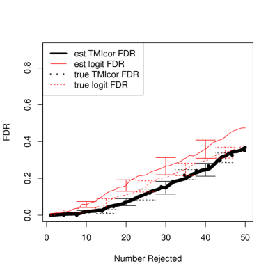
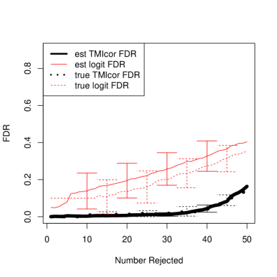
Within each class (diseased and healthy) we simulated 250250250 patients and applied TMIcor and the usual logistic approach. We averaged the true and estimated false discovery rates of these methods over 101010 trials. As we can see from Figure 1 TMIcor outperforms the logistic approach. This difference is particularly pronounced in the second plot of Figure 1. In this plot, because the correlations are large but different in both groups (ρ1=0.3subscript𝜌10.3\rho_{1}=0.3, ρ~1=0.6subscript~𝜌10.6\tilde{\rho}_{1}=0.6), there are some moderate quadratic effects in the true model — this induces a bias in the logistic approach and its FDR suffers. In contrast, these quadratic effects are not problematic in the backward framework.
Refer to caption Refer to caption

Figure 1: Plots of estimated and true FDR for TMIcor and logistic regression averaged over 101010 trials. Error bars contain the mean value ±plus-or-minus\pm 1 se of the mean. For controls, ρi=0.3subscript𝜌𝑖0.3\rho_{i}=0.3 for all i𝑖i. On the left ρ~1=0subscript~𝜌10\tilde{\rho}_{1}=0, while on the right ρ~1=0.6subscript~𝜌10.6\tilde{\rho}_{1}=0.6. There is no main effect in either panel.

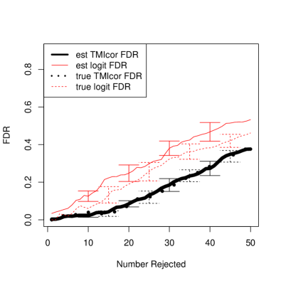
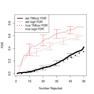
We also consider a second set of simulations. This set used ρi=0.3subscript𝜌𝑖0.3\rho_{i}=0.3 for all i𝑖i and ρ~1=0subscript~𝜌10\tilde{\rho}_{1}=0. However, instead of mean 00 in both classes, we set the mean for all proteins in block 1 for diseased patients to be some μ~1subscript~𝜇1\tilde{\mu}_{1} (>0absent0>0). The results are plotted in Figure 2. This mean shift had no effect on TMIcor (the procedure is meanshift invariant), but as the mean difference grows, it becomes increasingly difficult for the logistic regression to find any interactions. This issue is especially important as, biologically, one might expect that genes with main effects to be more likely to have true marginal interactions (and these interactions may also be more scientifically interesting).
Refer to caption Refer to caption

Figure 2: Plots of estimated and true FDR for TMIcor and logistic regression averaged over 101010 trials. Error bars contain the mean value ±plus-or-minus\pm 1 se of the mean. For both plots ρ~1=0subscript~𝜌10\tilde{\rho}_{1}=0 and ρi=0.3subscript𝜌𝑖0.3\rho_{i}=0.3 for all i𝑖i. Both panels have main effects — on the left μ~1μ1=0.5subscript~𝜇1subscript𝜇10.5\tilde{\mu}_{1}-\mu_{1}=0.5, while on the right μ~1μ1=1subscript~𝜇1subscript𝜇11\tilde{\mu}_{1}-\mu_{1}=1.

While these simulations are not exhaustive, they give an indication of a number of scenarios in which TMIcor significantly outperforms logistic regression. More exhaustive simulations were run and the results mirrored those in this section.

4.2 Real Data

We also applied both TMIcor and logistic regression to the colitis gene expression data of Burczynski et al. (2006). In this dataset, there are 127127127 total patients, 858585 with colitis (595959 Crohn’s patients + 262626 ulcerative colitis patients) and 424242 healthy controls. We restricted our analysis to the 101101101 patients without ulcerative colitis. Each patient had expression data for 222832228322283 genes run on an Affymetrix U133A microarray. Because chromosomes 555 and 101010 have been indicated in Crohn’s disease, we enriched our dataset by using only the genes on these chromosomes, along with the NOD2𝑁𝑂𝐷2NOD2 and ATG16L1𝐴𝑇𝐺16𝐿1ATG16L1 genes (chromosomes as specified by the C1𝐶1C1 geneset from Subramanian et al. (2005)). In total 663663663 genes were used. Some of these genes were measured by multiple probesets — the final expression values used for those genes were the average of all probesets.

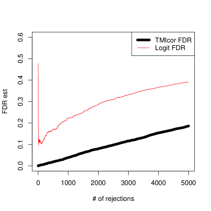
From these 663663663 genes we have 219,453219453219,453 of interactions to consider. Figure 3 shows the estimated FDR curves for the two methods. TMIcor finds many more significant interactions — at an FDR cutoff of 0.10.10.1, TMIcor finds 257025702570 significant interactions, while the logistic approach finds 151515. The significant 151515 from the logistic approach may not even be entirely believeable — the smallest p-value of the 151515 is roughly 1/21945312194531/219453, which is what we would expect it to be if all null hypotheses were true. Because the smallest p-value is large, we see that the FDR for logistic regression begins surprisingly high. The FDR subsequently drops because there are a number of p-values near the smallest, however, the significance of these hypotheses is still suspect.
Refer to caption

Figure 3: Corhn’s data; FDR estimates for TMIcor and logistic approaches for the 500050005000 most significant marginal interactions

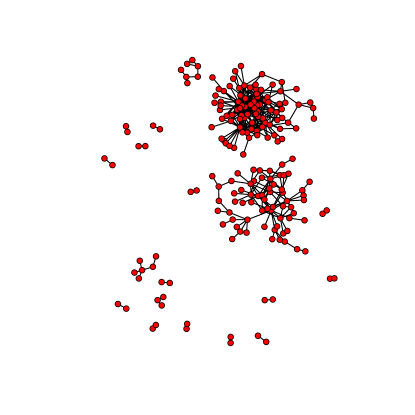
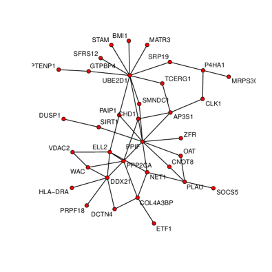
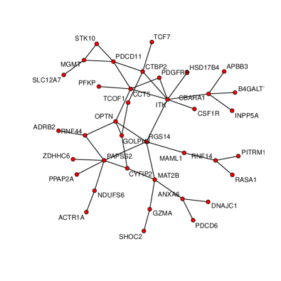
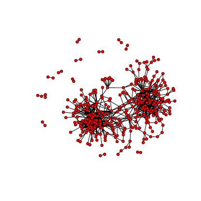
Unfortunately interpreting 257025702570 marginal interactions is difficult (even if all are true). Toward this end we consider the graphical representation of our analysis in Figure 4. Each gene is a node in our graph, and edges between genes signify marginal interactions. In this plot we considered only the 125012501250 of the 257025702570 significant marginal interactions indicative of a decrease in correlation from healthy control to Crohn’s (ie. Tj,k>0subscript𝑇𝑗𝑘0T_{j,k}>0). There is one large connected component, a few connected pairs and a large number of isolated genes. The connected component appears to be split into 222 clusters. To get a better handle on this, we considered a more stringent cutoff for significant interactions — at an FDR cutoff of 0.030.030.03, we are left with 832832832 significant interactions of which only 402402402 have Tj,k>0subscript𝑇𝑗𝑘0T_{j,k}>0. We plot this graph in Figure 5: we see that our large connected component has divided into 222. From here we further zoomed in on each component (now displaying only the 505050 most significant interactions per component), and can actually see which genes are are most important (in figure 6).
Refer to caption

Figure 4: Graph of 125012501250 marginal interactions (with decreasing correlation) significant at FDR cutoff of 0.10.10.1. Genes with no significant interactions not shown

Refer to caption

Figure 5: Graph of 402402402 marginal interactions (with decreasing correlation) significant at FDR cutoff of 0.030.030.03. Genes with no significant interactions not shown

Refer to caption Refer to caption

Figure 6: Graphs of the top 505050 marginal interactions in each cluster (and corresponding genes)

It appears, from this analysis, that there are two genetic pathways which are modified in Crohn’s disease. Many of the genes in each cluster are already known to be indicated in Crohn’s, but to our knowledge these interactions have not been considered.

5 Dealing with Nuisance Variables

Often, aside from the variables of interest, one may believe that other nuisance variables play a role in complex interactions. For example, it seems reasonable that many genes are conditionally independent given age, but are each highly correlated with age. Ignoring age, these genes would appear to be highly correlated, but this correlation is uninteresting to us. TMIcor can be adapted to deal with these nuisance variables provided there are few compared to the number of observations, they are continuous, and they are observed.

We resolve this issue by using partial correlations. Assume xjsubscript𝑥𝑗x_{j} and xksubscript𝑥𝑘x_{k} are our variables of interest, and z𝑧z is a vector of potential confounders. Rather than comparing cor(xj,xk)corsubscript𝑥𝑗subscript𝑥𝑘\operatorname{cor}\left(x_{j},x_{k}\right) in groups 111 and 222, we compare the partial correlations, cor([xj|z],[xk|z])cordelimited-[]conditionalsubscript𝑥𝑗𝑧delimited-[]conditionalsubscript𝑥𝑘𝑧\operatorname{cor}\left(\left[x_{j}|z\right],\left[x_{k}|z\right]\right). This is done by first regressing our potential confounders, Z𝑍Z, out of all the other features, then running the remainder of the analysis as usual.

To adapt the original algorithm in Section 3 to deal with nuisance variables we need only replace step (1)1(1) by:

  1. 1.

    Replace our feature matrices X1subscript𝑋1X_{1} and X2subscript𝑋2X_{2} by

    X~m=[IZm(ZmZm)Zm]Xmsubscript~𝑋𝑚delimited-[]𝐼subscript𝑍𝑚superscriptsubscript𝑍𝑚topsubscript𝑍𝑚superscriptsubscript𝑍𝑚topsubscript𝑋𝑚\tilde{X}_{m}=\left[I-Z_{m}\left(Z_{m}^{\top}Z_{m}\right)Z_{m}^{\top}\right]X_{m}

    Now, mean center and scale X~~𝑋\tilde{X} within each group.

We give more details motivating this approach and discussing potential computational advantages in appendix B.

6 Asymptotics

In this section we give two asymptotic results. We show that if n𝑛n\rightarrow\infty, and logpnn0subscript𝑝𝑛𝑛0\frac{\log p_{n}}{n}\rightarrow 0, then under certain regularity conditions our procedure for testing marginal interactions (in the absence of nuisance variables) is asymptotically consistent — with probability approaching 111 it calls significant all true marginal interactions and makes no false rejections. Furthermore, using the permutation null, it also consistently estimates that the true FDR is converging to 00. Because we only need logpnn0subscript𝑝𝑛𝑛0\frac{\log p_{n}}{n}\rightarrow 0, pnsubscript𝑝𝑛p_{n} may increase very rapidly in n𝑛n.

We first give a result showing that for sub-Gaussian variables our null statistics converge to 00 and our alternative statistics are asymptotically bounded away from 00. The proof of this theorem is based on several technical lemmas which we relegate to appendix C.

Theorem 6.1

Let x~1(j)subscript~𝑥1𝑗\tilde{x}_{1(j)} and x~2(j)subscript~𝑥2𝑗\tilde{x}_{2(j)}, j=1,𝑗1j=1,\ldots be random variables. Assume there is some C>0𝐶0C>0 such that for all t0𝑡0t\geq 0

P(|xm(j)E[xm(j)]|>t)exp(1t2/C2)Psubscript𝑥𝑚𝑗Esubscript𝑥𝑚𝑗𝑡exp1superscript𝑡2superscript𝐶2\operatorname{P}\left(\left|x_{m(j)}-\operatorname{E}[x_{m(j)}]\right|>t\right)\leq\operatorname{exp}\left(1-t^{2}/C^{2}\right)

for each m=1,2𝑚12m=1,2 . Let μi(j)subscript𝜇𝑖𝑗\mu_{i(j)} denote the mean of x~m(j)subscript~𝑥𝑚𝑗\tilde{x}_{m(j)} and σm(j)2superscriptsubscript𝜎𝑚𝑗2\sigma_{m(j)}^{2} its variance. For each i𝑖i\leq\infty, let xm(i,)subscript𝑥𝑚𝑖x_{m(i,\cdot)} be independent realizations with the same distribution as x~m()subscript~𝑥𝑚\tilde{x}_{m(\cdot)}.

Let pnsubscript𝑝𝑛p_{n} be a sequence of integers such that logpnn0subscript𝑝𝑛𝑛0\frac{\log p_{n}}{n}\rightarrow 0. Let Rmsubscript𝑅𝑚R_{m} be the correlation “matrix” (an infinite but countably indexed matrix) of the covariates from group m𝑚m. Let I𝐼I denote the set of ordered pairs (j,k)𝑗𝑘(j,k) for which R1(j,k)R2(j,k)subscript𝑅1𝑗𝑘subscript𝑅2𝑗𝑘R_{1(j,k)}\neq R_{2(j,k)}, and Cnsubscript𝐶𝑛C_{n} denote the set of ordered pairs (j,k)𝑗𝑘(j,k) with j,kpn𝑗𝑘subscript𝑝𝑛j,k\leq p_{n}.

Assume for every m𝑚m and j𝑗j, σm(j)2σmin2superscriptsubscript𝜎𝑚𝑗2superscriptsubscript𝜎𝑚𝑖𝑛2\sigma_{m(j)}^{2}\geq\sigma_{min}^{2} (for some σmin2>0superscriptsubscript𝜎𝑚𝑖𝑛20\sigma_{min}^{2}>0). Furthermore, assume that for all (j,k)𝑗𝑘(j,k) in each I𝐼I, |R1(j,k)R2(j,k)|>Δminsubscript𝑅1𝑗𝑘subscript𝑅2𝑗𝑘subscriptΔ\left|R_{1(j,k)}-R_{2(j,k)}\right|>\Delta_{\min} for some Δmin>0subscriptΔ0\Delta_{\min}>0 and that for m=1,2𝑚12m=1,2, supj<k|Rm(j,k)|<ρmaxsubscriptsup𝑗𝑘subscript𝑅𝑚𝑗𝑘subscript𝜌\operatorname{sup}_{j<k}\left|R_{m(j,k)}\right|<\rho_{\max} for some fixed ρmax<1subscript𝜌1\rho_{\max}<1.

Now, given any ϵp>0subscriptitalic-ϵ𝑝0\epsilon_{p}>0, and 0<t<Δmin0𝑡subscriptΔ0<t<\Delta_{\min}, if we choose n𝑛n sufficiently large, then with probability at least 1ϵp1subscriptitalic-ϵ𝑝1-\epsilon_{p}

|T(j,k)|tsubscript𝑇𝑗𝑘𝑡\left|T_{(j,k)}\right|\leq t

for all (j,k)𝑗𝑘(j,k) in CnIsubscript𝐶𝑛𝐼C_{n}-I, and

|T(j,k)|tsubscript𝑇𝑗𝑘𝑡\left|T_{(j,k)}\right|\geq t

for all (j,k)𝑗𝑘(j,k) in CnIsubscript𝐶𝑛𝐼C_{n}\cap I.

The notation here is a little bit tricky, but the result is very straightforward: under some simple conditions, we find all marginal interactions and make no false identifications.

While there were a number of assumptions in the above theorem, most of these are fairly trivial and will almost always be found in practice: the variance must be bounded away from 00 and the correlations bounded away from ±1plus-or-minus1\pm 1. The assumption that the correlation differences are bounded below by a fixed ΔminsubscriptΔ\Delta_{\min} for true marginal interactions is a bit more cumbersome, but may easily be relaxed to Δmin0subscriptΔ0\Delta_{\min}\rightarrow 0 at a slow enough rate that Δmin/[logp/n]1/2subscriptΔ𝑚𝑖𝑛superscriptdelimited-[]𝑝𝑛12\Delta_{min}/\left[\log p/n\right]^{1/2}\rightarrow\infty.

The astute reader might note that our assumption bounding the variance away from 00 seems strange — the distribution of the sample correlation is independent of the variance. This is necessary only because we assumed the covariates have a subgaussian tail with a shared constant C𝐶C. One could have relaxed the bounded variance assumption to the assumption that {xj/σj}j=1,subscriptsubscript𝑥𝑗subscript𝜎𝑗𝑗1\left\{x_{j}/\sigma_{j}\right\}_{j=1,\ldots} have a sub-Gaussian tail with a shared constant C𝐶C.

6.1 Permutation Consistency

Now that we have shown our procedure has FDR converging to 00, we would like to show that it asymptotically estimates FDR consistently as well. In particular we show that as n𝑛n\rightarrow\infty, if logpn0𝑝𝑛0\frac{\log p}{n}\rightarrow 0, then with probability approaching 111, for a random permutation, our permuted statistics converge to 00 uniformly in probability (maxj,k|T(j,k)|tsubscript𝑗𝑘superscriptsubscript𝑇𝑗𝑘𝑡\max_{j,k}\left|T_{(j,k)}^{*}\right|\leq t for any fixed t>0𝑡0t>0 with probability converging to 111). Thus our estimated FDR converges to 00 under the same conditions as our true FDR.

We begin with some notation. Let us consider an arbitrary permutation of class labels, ΠΠ\Pi. Let π^^𝜋\hat{\pi} denote the proportion of observations from class 111 that remain in class 111 after permuting.

We discuss a somewhat simplified procedure in our proof, as otherwise the algebra becomes significantly more painful (without any added value in clarity), but it is straightforward to carry the proof through to the full procedure. In our original procedure, after permuting class labels we recenter and rescale our variables within each class. Because we already centered and scaled variables before permuting, this step will have very little effect on our procedure (though it does have the nice effect of never giving |ρ|>1superscript𝜌1|\rho^{*}|>1). In this proof we consider a procedure identical in every way except without recentering and rescaling within each permutation.

Before we give the theorem, we would like to define a few new terms for clarity. For a given permutation ΠΠ\Pi, let Πi(m){0,1}subscriptΠ𝑖𝑚01\Pi_{i}(m)\in\left\{0,1\right\} be the permuted class of the i𝑖i-th observation originally in class m𝑚m. Furthermore, let Π(m,l)Π𝑚𝑙\Pi\left(m,l\right) be the set of observations in class m𝑚m that are permuted to class l𝑙l, and let Π(,l)Π𝑙\Pi\left(\cdot,l\right) be the set of observations in both classes permuted to class l𝑙l, ie.

Π(m,l)Π𝑚𝑙\displaystyle\Pi\left(m,l\right) ={i:Πi(m)=l}absentconditional-set𝑖subscriptΠ𝑖𝑚𝑙\displaystyle=\left\{i:\,\Pi_{i}(m)=l\right\}
Π(,l)Π𝑙\displaystyle\Pi\left(\cdot,l\right) ={(i,m):Πi(m)=l}absentconditional-set𝑖𝑚subscriptΠ𝑖𝑚𝑙\displaystyle=\left\{(i,m):\,\Pi_{i}(m)=l\right\}

Now, we give a result which shows that for any fixed t>0𝑡0t>0 if our variables are sub-Gaussian with some other minor conditions, then for n𝑛n\rightarrow\infty and logp/n0𝑝𝑛0\log p/n\rightarrow 0 with probability approaching 111, none of our permuted statistics will be larger than t𝑡t, or in other words, as our true converged to 00, so will our estimated FDR 00. As before, the proof of this theorem is based on several technical lemmas which we again leave to appendix C.

Theorem 6.2

Let x~1(j)subscript~𝑥1𝑗\tilde{x}_{1(j)} and x~2(j)subscript~𝑥2𝑗\tilde{x}_{2(j)}, j=1,𝑗1j=1,\ldots be random variables with

P(|xm(j)E[xm(j)]|t)1et2/CPsubscript𝑥𝑚𝑗Esubscript𝑥𝑚𝑗𝑡1superscript𝑒superscript𝑡2𝐶\operatorname{P}\left(|x_{m(j)}-\operatorname{E}\left[x_{m(j)}\right]|\geq t\right)\leq 1-e^{t^{2}/C}

for all t>0𝑡0t>0, and each m=1,2𝑚12m=1,2, with some fixed C>0𝐶0C>0. Let μm(j)subscript𝜇𝑚𝑗\mu_{m(j)} denote the mean of x~m(j)subscript~𝑥𝑚𝑗\tilde{x}_{m(j)} and σm(j)2superscriptsubscript𝜎𝑚𝑗2\sigma_{m(j)}^{2} its variance. For each i𝑖i\leq\infty, let xm(i,)subscript𝑥𝑚𝑖x_{m(i,\cdot)} be independent realizations with the same distribution as x~m()subscript~𝑥𝑚\tilde{x}_{m(\cdot)}.

Let pnsubscript𝑝𝑛p_{n} be a sequence of integers such that logpnn0subscript𝑝𝑛𝑛0\frac{\log p_{n}}{n}\rightarrow 0. Let Rmsubscript𝑅𝑚R_{m} be the correlation “matrix” (an infinite but countably indexed matrix) of the covariates from class m𝑚m.

Assume for every m,j𝑚𝑗m,\,j, σm(j)2σmin2superscriptsubscript𝜎𝑚𝑗2superscriptsubscript𝜎𝑚𝑖𝑛2\sigma_{m(j)}^{2}\geq\sigma_{min}^{2} (for some σmin2>0superscriptsubscript𝜎𝑚𝑖𝑛20\sigma_{min}^{2}>0). Furthermore, assume that for m=1,2𝑚12m=1,2, supj<k|Rm(j,k)|<ρmaxsubscriptsup𝑗𝑘subscript𝑅𝑚𝑗𝑘subscript𝜌\operatorname{sup}_{j<k}\left|R_{m(j,k)}\right|<\rho_{\max} for some fixed ρmax<1subscript𝜌1\rho_{\max}<1.

Now, given any ϵp>0subscriptitalic-ϵ𝑝0\epsilon_{p}>0, and 0<t0𝑡0<t, if we choose n𝑛n sufficiently large and let ΠΠ\Pi be a random permutation, then with probability at least 1ϵp1subscriptitalic-ϵ𝑝1-\epsilon_{p}

|T(j,k)|tsuperscriptsubscript𝑇𝑗𝑘𝑡\left|T_{(j,k)}^{*}\right|\leq t

for all (j,k)𝑗𝑘(j,k) with j,kpn𝑗𝑘subscript𝑝𝑛j,k\leq p_{n} where

T(j,k)=arctanh(R^perm:1(j,k))arctanh(R^perm:2(j,k))superscriptsubscript𝑇𝑗𝑘arctanhsubscript^𝑅:perm1jkarctanhsubscript^𝑅:perm2jkT_{(j,k)}^{*}=\operatorname{arctanh}\left(\hat{R}_{\operatorname{perm:1(j,k)}}\right)-\operatorname{arctanh}\left(\hat{R}_{\operatorname{perm:2(j,k)}}\right)

and

R^perm:m(j,k)=1n(i,l)Π(,m)(xl(i,j)μ^l(j)σ^l(j))(xm(i,k)μ^l(k)σ^l(k))subscript^𝑅:perm𝑚𝑗𝑘1𝑛subscript𝑖𝑙Π𝑚subscript𝑥𝑙𝑖𝑗subscript^𝜇𝑙𝑗subscript^𝜎𝑙𝑗subscript𝑥𝑚𝑖𝑘subscript^𝜇𝑙𝑘subscript^𝜎𝑙𝑘\hat{R}_{\textrm{perm}:m(j,k)}=\frac{1}{n}\sum_{(i,l)\in\Pi(\cdot,m)}\left(\frac{x_{l(i,j)}-\hat{\mu}_{l(j)}}{\hat{\sigma}_{l(j)}}\right)\left(\frac{x_{m(i,k)}-\hat{\mu}_{l(k)}}{\hat{\sigma}_{l(k)}}\right)

The notation is again somewhat ugly, but the result is very straightforward: under some simple conditions, our permuted statistics are very small. In particular from the proof one can see that sup{T(j,k)}=Op(logpn/n)supsuperscriptsubscript𝑇𝑗𝑘subscript𝑂𝑝subscript𝑝𝑛𝑛\operatorname{sup}\left\{T_{(j,k)}^{*}\right\}=O_{p}\left(\sqrt{\log p_{n}/n}\right).

Note there is an implicit indexing of n𝑛n in R^perm:m(j,k)subscript^𝑅:perm𝑚𝑗𝑘\hat{R}_{\textrm{perm}:m(j,k)} (it seemed unneccessary to add more indices). As in theorem 6.1, some of our conditions may be relaxed. Instead of bounding σj2superscriptsubscript𝜎𝑗2\sigma_{j}^{2} below, we need only bound Cσj𝐶subscript𝜎𝑗C\sigma_{j} below. Also, rather than choose a fixed cutoff, t>0𝑡0t>0, we may use any sequence {tn}subscript𝑡𝑛\left\{t_{n}\right\} with tn/(logpn/n)1/2subscript𝑡𝑛superscriptsubscript𝑝𝑛𝑛12t_{n}/\left(\log p_{n}/n\right)^{1/2}\rightarrow\infty. Also, as noted before, the result we have just shown ignores the restandardizing within each permutation, however it is straightforward (though algebraicly arduous, and not insightful) to extend this result to that case as well.

As a last note, in theorem 6.2, we gave our consistency result for only a single permutation. This result can easily be extended to any fixed number of permutations using a union bound. This was left out of the original statement/proof as the notation is already clunky and the extension is straightforward.

Through theorems 6.1 and 6.2 we have shown that, under fairly relaxed conditions, our procedure is asymptotically consistent at discovering marginal interactions and that the permutation null reflects this.

7 Discussion

In this paper we have discussed marginal interactions for logistic regression in the framework of forward and backward models. We have developed a permutation based method, TMIcor, which leverages the backward model. We have shown its efficacy on real and simulated data and given asymptotic results showing its consistency and convergence rate. We also plan to release a publically available R implementation.

8 Appendix A

In this section we give more details on our permutation-based estimate of FDR, and discuss a potential alternative. Recall that we are using the permutations to approximate

(j,k) nullP(|T(j,k)|>t).subscript𝑗𝑘 nullPsubscript𝑇𝑗𝑘𝑡\sum_{(j,k)\textrm{ null}}\operatorname{P}(|T_{(j,k)}|>t). (6)

For the moment, assume that all covariates in both classes have mean 00 and variance 111, and that we did not do any sample standarization. Then, under the null hypothesis that R1(j,k)=R2(j,k)subscript𝑅1𝑗𝑘subscript𝑅2𝑗𝑘R_{1(j,k)}=R_{2(j,k)}, T(j,k)subscript𝑇𝑗𝑘T_{(j,k)} calculated under the original class assignments and T(j,k)subscriptsuperscript𝑇𝑗𝑘T^{*}_{(j,k)} calculated under any permuted class assignments have the same distribution, so

(j,k) nullP(|T(j,k)|>t)=(j,k) nullP(|T(j,k)|>t)subscript𝑗𝑘 nullPsubscript𝑇𝑗𝑘𝑡subscript𝑗𝑘 nullPsubscriptsuperscript𝑇𝑗𝑘𝑡\sum_{(j,k)\textrm{ null}}\operatorname{P}(|T_{(j,k)}|>t)=\sum_{(j,k)\textrm{ null}}\operatorname{P}(|T^{*}_{(j,k)}|>t)

which is reasonably (and unbiasedly) approximated by

(j,k) null1Aa=1AI(|T(j,k)a|>t).subscript𝑗𝑘 null1𝐴superscriptsubscript𝑎1𝐴𝐼subscriptsuperscript𝑇absent𝑎𝑗𝑘𝑡\sum_{(j,k)\textrm{ null}}\frac{1}{A}\sum_{a=1}^{A}I(|T^{*a}_{(j,k)}|>t).

Because we do not know which genes are null, our actual estimate of (6) is

(j,k)1Aa=1AI(|T(j,k)a|>t)subscript𝑗𝑘1𝐴superscriptsubscript𝑎1𝐴𝐼subscriptsuperscript𝑇absent𝑎𝑗𝑘𝑡\displaystyle\sum_{(j,k)}\frac{1}{A}\sum_{a=1}^{A}I(|T^{*a}_{(j,k)}|>t) =(j,k) null1Aa=1AI(|T(j,k)a|>t)absentsubscript𝑗𝑘 null1𝐴superscriptsubscript𝑎1𝐴𝐼subscriptsuperscript𝑇absent𝑎𝑗𝑘𝑡\displaystyle=\sum_{(j,k)\textrm{ null}}\frac{1}{A}\sum_{a=1}^{A}I(|T^{*a}_{(j,k)}|>t) (7)
+(j,k) alternative1Aa=1AI(|T(j,k)a|>t)subscript𝑗𝑘 alternative1𝐴superscriptsubscript𝑎1𝐴𝐼subscriptsuperscript𝑇absent𝑎𝑗𝑘𝑡\displaystyle+\sum_{(j,k)\textrm{ alternative}}\frac{1}{A}\sum_{a=1}^{A}I(|T^{*a}_{(j,k)}|>t) (8)

This gives a slight conservative bias (especially small if most marginal interactions are null). One should also note that unlike the null statistics, for the alternative (j,k)𝑗𝑘(j,k), T(j,k)subscriptsuperscript𝑇𝑗𝑘T^{*}_{(j,k)} are not distributed N(0,2n3)𝑁02𝑛3N\left(0,\frac{2}{n-3}\right); they are still mean 00, but the variance is increased. However, this conservative bias is very slight — in general there are few alternative hypotheses, and the variance increase is not large.

Because in practice we do not have mean 00, variance 111 for all covariates in both classes, we must standardize before running our procedure. Otherwise, instead of testing for a changing correlation, we are actually testing for a different mean, variance, or correlation between classes. The effect of standardizing with the sample mean and variance rather than the true values is asymptotically washed out, and while the variance of our tests is increased for small samples, this increase is only minimal.

An alternative to permutations, as discussed in Efron (2010), is to directly estimate the numerator using the approximate theoretical distribution of the null statistics. Each null statistic is asymptotically N(0,1n13+1n23)𝑁01subscript𝑛131subscript𝑛23N\left(0,\frac{1}{n_{1}-3}+\frac{1}{n_{2}-3}\right), so for (j,k)𝑗𝑘(j,k) null

P(|T(j,k)|>t)=2Φ(t(n13)(n23)n1+n26).Psubscript𝑇𝑗𝑘𝑡2Φ𝑡subscript𝑛13subscript𝑛23subscript𝑛1subscript𝑛26\operatorname{P}(|T_{(j,k)}|>t)=2\Phi\left(-\frac{t(n_{1}-3)(n_{2}-3)}{n_{1}+n_{2}-6}\right).

Now we can conservatively approximate the quantity in Eq (6) by

(j,k) nullP(|T(j,k)|>t)subscript𝑗𝑘 null𝑃subscript𝑇𝑗𝑘𝑡\displaystyle\sum_{(j,k)\textrm{ null}}P\left(|T_{(j,k)}|>t\right) p(p1)/2P(|Tnull|>t)absent𝑝𝑝12𝑃subscript𝑇null𝑡\displaystyle\leq p(p-1)/2\cdot P\left(|T_{\textrm{null}}|>t\right)
=p(p1)Φ(t(n13)(n23)n1+n26)absent𝑝𝑝1Φ𝑡subscript𝑛13subscript𝑛23subscript𝑛1subscript𝑛26\displaystyle=p(p-1)\cdot\Phi\left(-\frac{t(n_{1}-3)(n_{2}-3)}{n_{1}+n_{2}-6}\right)

While this approach is reasonable and simple, it is less robust than using permutations, and in practice, even for truly Gaussian data, it is only slightly more efficient.

9 Appendix B

Before proceeding, we remind the reader that x𝑥x are our variables of interest and z𝑧z are potential confounding variables. Furthermore we are interested in comparing cor([xj|z],[xk|z])cordelimited-[]conditionalsubscript𝑥𝑗𝑧delimited-[]conditionalsubscript𝑥𝑘𝑧\operatorname{cor}\left(\left[x_{j}|z\right],\left[x_{k}|z\right]\right) between groups. From basic properties of the Gaussian distribution we know that

x|zN[μx+Σ(x,z)Σz1(zμz),Σ(x|z)]similar-toconditional𝑥𝑧𝑁subscript𝜇𝑥subscriptΣ𝑥𝑧superscriptsubscriptΣ𝑧1𝑧subscript𝜇𝑧subscriptΣconditional𝑥𝑧x|z\sim N\left[\mu_{x}+\Sigma_{(x,z)}\Sigma_{z}^{-1}\left(z-\mu_{z}\right),\Sigma_{(x|z)}\right]

where Σ(x|z)subscriptΣconditional𝑥𝑧\Sigma_{(x|z)} is the variance/covariance matrix of x𝑥x given z𝑧z, Σ(x,z)subscriptΣ𝑥𝑧\Sigma_{(x,z)} is the covariance matrix between x𝑥x and z𝑧z, ΣzsubscriptΣ𝑧\Sigma_{z} is the variance matrix of z𝑧z, and μxsubscript𝜇𝑥\mu_{x} and μzsubscript𝜇𝑧\mu_{z} are the means of x𝑥x and z𝑧z. Now, if μx,μz,Σ(x,z),subscript𝜇𝑥subscript𝜇𝑧subscriptΣ𝑥𝑧\mu_{x},\,\mu_{z},\,\Sigma_{(x,z)}, and ΣzsubscriptΣ𝑧\Sigma_{z} were known, then the MLE for Σ(x|z)subscriptΣconditional𝑥𝑧\Sigma_{(x|z)} would be

Σ^(x|z)=1n[X1μx(Z1μz)Σz1Σ(z,x)][X1μX(Z1μZ)ΣZ1Σ(z,x)].subscript^Σconditional𝑥𝑧1𝑛superscriptdelimited-[]𝑋1superscriptsubscript𝜇𝑥top𝑍1superscriptsubscript𝜇𝑧topsuperscriptsubscriptΣ𝑧1subscriptΣ𝑧𝑥topdelimited-[]𝑋1superscriptsubscript𝜇𝑋top𝑍1superscriptsubscript𝜇𝑍topsuperscriptsubscriptΣ𝑍1subscriptΣ𝑧𝑥\hat{\Sigma}_{(x|z)}=\frac{1}{n}\left[X-1\mu_{x}^{\top}-\left(Z-1\mu_{z}^{\top}\right)\Sigma_{z}^{-1}\Sigma_{(z,x)}\right]^{\top}\left[X-1\mu_{X}^{\top}-\left(Z-1\mu_{Z}^{\top}\right)\Sigma_{Z}^{-1}\Sigma_{(z,x)}\right].

Unfortunately, these nuisance parameters are unknown. However we can also estimate them by maximum likelihood. This gives us the estimate

Σ^(X|Z)subscript^Σconditional𝑋𝑍\displaystyle\hat{\Sigma}_{(X|Z)} =1n[X~Z~(Z~Z~)1Z~X~][X~Z~(Z~Z~)1Z~X~]absent1𝑛superscriptdelimited-[]~𝑋~𝑍superscriptsuperscript~𝑍top~𝑍1superscript~𝑍top~𝑋topdelimited-[]~𝑋~𝑍superscriptsuperscript~𝑍top~𝑍1superscript~𝑍top~𝑋\displaystyle=\frac{1}{n}\left[\tilde{X}-\tilde{Z}\left(\tilde{Z}^{\top}\tilde{Z}\right)^{-1}\tilde{Z}^{\top}\tilde{X}\right]^{\top}\left[\tilde{X}-\tilde{Z}\left(\tilde{Z}^{\top}\tilde{Z}\right)^{-1}\tilde{Z}^{\top}\tilde{X}\right]
=1n[PZ~(X~)][PZ~(X~)]absent1𝑛superscriptdelimited-[]subscriptPperpendicular-to~𝑍absent~𝑋topdelimited-[]subscriptPperpendicular-to~𝑍absent~𝑋\displaystyle=\frac{1}{n}\left[\operatorname{P}_{\tilde{Z}\perp}\left(\tilde{X}\right)\right]^{\top}\left[\operatorname{P}_{\tilde{Z}\perp}\left(\tilde{X}\right)\right]

where Z~~𝑍\tilde{Z} is the standardized version of Z𝑍Z, and X~~𝑋\tilde{X} is the standardized version of X𝑋X, and PZ~subscriptPperpendicular-to~𝑍absent\operatorname{P}_{\tilde{Z}\perp} is the projection onto the orthogonal complement of the column space of Z~~𝑍\tilde{Z}. So, our estimate of partial correlation is just an estimate of correlation with Z𝑍Z regressed out of both covariates. We use this to contruct our permutation null. In the orginal algorithm, we mean centered and scaled before permuting; here we do the equivalent — we project our variables of interest onto the orthogonal complement of our nuisance variables, and then center/scale them. Now we are ready to permute. We permute these “residuals”, and calculate permuted correlations as before.

Before proceeding, we note that for n𝑛n sufficiently large n𝑛n (n>>pmuch-greater-than𝑛𝑝n>>p) one might use a similar approach to consider partial correlations rather than marginal correlations in our original algorithm (conditioning out all covariates except any particular 222). However, in general n<<pmuch-less-than𝑛𝑝n<<p and thus P0subscriptPperpendicular-to0\operatorname{P}_{\perp}\equiv 0 rendering this approach ineffective — this approach only works for nuisance variables because we assume that there are very few relative to the number of observations.

As stated in the text, to adapt the original algorithm to deal with nuisance variables we need only replace step (1)1(1) by:

  1. 1.

    Replace our feature matrices X1subscript𝑋1X_{1} and X2subscript𝑋2X_{2} by

    X~m=[IZm(ZmZm)Zm]Xmsubscript~𝑋𝑚delimited-[]𝐼subscript𝑍𝑚superscriptsubscript𝑍𝑚topsubscript𝑍𝑚superscriptsubscript𝑍𝑚topsubscript𝑋𝑚\tilde{X}_{m}=\left[I-Z_{m}\left(Z_{m}^{\top}Z_{m}\right)Z_{m}^{\top}\right]X_{m}

    Now, mean center and scale X~~𝑋\tilde{X} within each group.

One may note that we only calculate X~~𝑋\tilde{X} once per class, at the beginning of our procedure, not in each permutation. We do this for a similar reason that we standardize our variables before permuting — because we are not testing the hypothesis that the relationship between X𝑋X and Z𝑍Z is the same in both groups. If we relcalulate after each permutation then we are implicitly assuming that this relationship is the same in both groups under the null.

Even with nuisance variables this approach is very computationally fast. Projecting our original variables onto Zperpendicular-to𝑍absentZ\perp can be done in O(nppnuis)𝑂𝑛𝑝subscript𝑝nuisO\left(npp_{\textrm{nuis}}\right) operations where pnuissubscript𝑝nuisp_{\textrm{nuis}} is the number of nuisance variables. Thus the total runtime of this algorithm is O(nppnuis+Anp(p1)/2)𝑂𝑛𝑝subscript𝑝nuis𝐴𝑛𝑝𝑝12O\left(npp_{\textrm{nuis}}+Anp(p-1)/2\right) where A𝐴A is the number of permutations — this is dominated by the second term, which is independent of the number of nuisance parameters. In contrast, if we were to use the standard approach (fitting pairwise logistic regressions with nuisance variables), its runtime would be O[(iter)(3+pnuis)2np(p1)/2]𝑂delimited-[]𝑖𝑡𝑒𝑟superscript3subscript𝑝nuis2𝑛𝑝𝑝12O\left[\left(iter\right)(3+p_{\textrm{nuis}})^{2}np(p-1)/2\right] where iter𝑖𝑡𝑒𝑟iter is the number of iterations of the algorithm for finding the MLE. In general A100similar-to𝐴100A\sim 100 and iter5similar-to𝑖𝑡𝑒𝑟5iter\sim 5. Now, since (3+pnuis)2superscript3subscript𝑝nuis2(3+p_{\textrm{nuis}})^{2} grows very quickly in pnuissubscript𝑝nuisp_{\textrm{nuis}}, for even a small number of nuisance parameters the logistic approach becomes much slower.

10 Appendix C

This appendix contains the technical details from the theorems in section 777 of the main manuscript. We begin with a number of technical lemmas:

First, as one might imagine, if we can consistently estimate our correlation matrices, applying a Fisher transformation should not change much. We formalize this with the next lemma.

Lemma 10.1

Let R1subscript𝑅1R_{1}, R2subscript𝑅2R_{2} be correlation matrices, and R^1subscript^𝑅1\hat{R}_{1}, R^2subscript^𝑅2\hat{R}_{2} be estimates of R1subscript𝑅1R_{1} and R2subscript𝑅2R_{2}.

Let I𝐼I be the set of ordered pairs (j,k)𝑗𝑘(j,k) where R1(j,k)R2(j,k)subscript𝑅1𝑗𝑘subscript𝑅2𝑗𝑘R_{1(j,k)}\neq R_{2(j,k)}. Assume for all (j,k)𝑗𝑘(j,k) in I𝐼I, |R1(j,k)R2(j,k)|>Δminsubscript𝑅1𝑗𝑘subscript𝑅2𝑗𝑘subscriptΔ\left|R_{1(j,k)}-R_{2(j,k)}\right|>\Delta_{\min} for some Δmin>0subscriptΔ0\Delta_{\min}>0 and that for m=1,2𝑚12m=1,2 we have supj<kRm(j,k)<ρmaxsubscriptsup𝑗𝑘subscriptnormsubscript𝑅𝑚𝑗𝑘subscript𝜌\operatorname{sup}_{j<k}\left\|R_{m(j,k)}\right\|_{\infty}<\rho_{\max} for some fixed ρmax<1subscript𝜌1\rho_{\max}<1.

Further assume that for m=1,2𝑚12m=1,2, RmR^mδsubscriptnormsubscript𝑅𝑚subscript^𝑅𝑚𝛿\left\|R_{m}-\hat{R}_{m}\right\|_{\infty}\leq\delta (for some δ<1ρmax𝛿1subscript𝜌\delta<1-\rho_{\max}). Then for all (j,k)𝑗𝑘(j,k) in Icsuperscript𝐼𝑐I^{c} with jk𝑗𝑘j\neq k we have

|arctanh(R^1(j,k))arctanh(R^2(j,k))|2δ1(ρmax+δ)2arctanhsubscript^𝑅1𝑗𝑘arctanhsubscript^𝑅2𝑗𝑘2𝛿1superscriptsubscript𝜌𝛿2\left|\operatorname{arctanh}\left(\hat{R}_{1(j,k)}\right)-\operatorname{arctanh}\left(\hat{R}_{2(j,k)}\right)\right|\leq\frac{2\delta}{1-\left(\rho_{\max}+\delta\right)^{2}} (9)

and for all (j,k)𝑗𝑘(j,k) in I𝐼I with jk𝑗𝑘j\neq k we have

|arctanh(R^1(j,k))arctanh(R^2(j,k))|Δmin2δarctanhsubscript^𝑅1𝑗𝑘arctanhsubscript^𝑅2𝑗𝑘subscriptΔ2𝛿\left|\operatorname{arctanh}\left(\hat{R}_{1(j,k)}\right)-\operatorname{arctanh}\left(\hat{R}_{2(j,k)}\right)\right|\geq\Delta_{\min}-2\delta (10)

One immediate consequence of this lemma is that as δ0𝛿0\delta\rightarrow 0, for (j,k)𝑗𝑘(j,k) in ICsuperscript𝐼𝐶I^{C} our statistics T(j,k)subscript𝑇𝑗𝑘T_{(j,k)} converge to 00 (at rate O(δ)\delta)), and for (j,k)𝑗𝑘(j,k) in I𝐼I, T(j,k)subscript𝑇𝑗𝑘T_{(j,k)} are bounded away from 00 (at a rate of at least O(δ)\delta)).

Proof 10.2 (Proof of Lemma 10.1)

We begin by showing that for all (j,k)𝑗𝑘(j,k) in Icsuperscript𝐼𝑐I^{c} with jk𝑗𝑘j\neq k we have

|arctanh(R^1(j,k))arctanh(R^2(j,k))|2δ1(ρmax+δ)2arctanhsubscript^𝑅1𝑗𝑘arctanhsubscript^𝑅2𝑗𝑘2𝛿1superscriptsubscript𝜌𝛿2\left|\operatorname{arctanh}\left(\hat{R}_{1(j,k)}\right)-\operatorname{arctanh}\left(\hat{R}_{2(j,k)}\right)\right|\leq\frac{2\delta}{1-\left(\rho_{\max}+\delta\right)^{2}}

The mean value theorem gives us that

|arctanh(R^1(j,k))arctanh(R^2(j,k))|supr|11r2||R^1(j,k)R^2(j,k)|arctanhsubscript^𝑅1𝑗𝑘arctanhsubscript^𝑅2𝑗𝑘subscriptsup𝑟11superscript𝑟2subscript^𝑅1𝑗𝑘subscript^𝑅2𝑗𝑘\left|\operatorname{arctanh}\left(\hat{R}_{1(j,k)}\right)-\operatorname{arctanh}\left(\hat{R}_{2(j,k)}\right)\right|\leq\operatorname{sup}_{r}\left|\frac{1}{1-r^{2}}\right|\left|\hat{R}_{1(j,k)}-\hat{R}_{2(j,k)}\right|

where the supremum is taken over r𝑟r in [R^1(j,k),R^2(j,k)]subscript^𝑅1𝑗𝑘subscript^𝑅2𝑗𝑘\left[\hat{R}_{1(j,k)},\,\hat{R}_{2(j,k)}\right]. Note that for m=1,2𝑚12m=1,2, we have |R^m(j,k)|<ρmax+δsubscript^𝑅𝑚𝑗𝑘subscript𝜌𝛿|\hat{R}_{m(j,k)}|<\rho_{\max}+\delta, and |R^1(j,k)R^2(j,k)|2δsubscript^𝑅1𝑗𝑘subscript^𝑅2𝑗𝑘2𝛿\left|\hat{R}_{1(j,k)}-\hat{R}_{2(j,k)}\right|\leq 2\delta, for (j,k)𝑗𝑘(j,k) not in I𝐼I. Thus,

supr|11r2||R^1(j,k)R^2(j,k)|2δ1(ρmax+δ)2.subscriptsup𝑟11superscript𝑟2subscript^𝑅1𝑗𝑘subscript^𝑅2𝑗𝑘2𝛿1superscriptsubscript𝜌𝛿2\operatorname{sup}_{r}\left|\frac{1}{1-r^{2}}\right|\left|\hat{R}_{1(j,k)}-\hat{R}_{2(j,k)}\right|\leq\frac{2\delta}{1-\left(\rho_{\max}+\delta\right)^{2}}.

Now for (j,k)𝑗𝑘(j,k) in I𝐼I, we again use the mean value theorem:

|arctanh(R^1(j,k))arctanh(R^2(j,k))|infr|11r2||R^1(j,k)R^2(j,k)|arctanhsubscript^𝑅1𝑗𝑘arctanhsubscript^𝑅2𝑗𝑘subscriptinf𝑟11superscript𝑟2subscript^𝑅1𝑗𝑘subscript^𝑅2𝑗𝑘\left|\operatorname{arctanh}\left(\hat{R}_{1(j,k)}\right)-\operatorname{arctanh}\left(\hat{R}_{2(j,k)}\right)\right|\geq\operatorname{inf}_{r}\left|\frac{1}{1-r^{2}}\right|\left|\hat{R}_{1(j,k)}-\hat{R}_{2(j,k)}\right|

and our result follows because |R^1(j,k)R^2(j,k)|Δmin2δsubscript^𝑅1𝑗𝑘subscript^𝑅2𝑗𝑘subscriptΔ2𝛿\left|\hat{R}_{1(j,k)}-\hat{R}_{2(j,k)}\right|\geq\Delta_{\min}-2\delta.

Now we consider convergence of these sample correlation matrices. We show that their convergence depends only on the convergence of the sample means (μ^jsubscript^𝜇𝑗\hat{\mu}_{j}), variances (σ^j2superscriptsubscript^𝜎𝑗2\hat{\sigma}_{j}^{2}), and pairwise inner products. We formalize this in the following lemma.

Lemma 10.3

Let x~jsubscript~𝑥𝑗\tilde{x}_{j}, j=1,𝑗1j=1,\ldots be random variables. Let μjsubscript𝜇𝑗\mu_{j} denote the mean of x~jsubscript~𝑥𝑗\tilde{x}_{j} and σj2superscriptsubscript𝜎𝑗2\sigma_{j}^{2} its variance. Let Rj,ksubscript𝑅𝑗𝑘R_{j,k} be the correlation between x~jsubscript~𝑥𝑗\tilde{x}_{j} and x~ksubscript~𝑥𝑘\tilde{x}_{k}. For each i𝑖i, let xi,subscript𝑥𝑖x_{i,\cdot} be independent realizations with the same distribution as x~subscript~𝑥\tilde{x}_{\cdot} (eg. xi,jsubscript𝑥𝑖𝑗x_{i,j} has the marginal distribution of x~jsubscript~𝑥𝑗\tilde{x}_{j}).

For any given ϵ>0italic-ϵ0\epsilon>0, there exists δ>0𝛿0\delta>0 such that if

sup{|σ^jσj|,|μ^jμj|,|(1/n)inxi,jxi,kσjσkμjμkσjσkRj,k|}j,kδ\operatorname{sup}\left\{\left|\hat{\sigma}_{j}-\sigma_{j}\right|,\,\left|\hat{\mu}_{j}-\mu_{j}\right|,\,\left|\frac{(1/n)\sum_{i\leq n}x_{i,j}x_{i,k}}{\sigma_{j}\sigma_{k}}-\frac{\mu_{j}\mu_{k}}{\sigma_{j}\sigma_{k}}-R_{j,k}\right|\right\}_{j,k}\leq\delta (11)

then

supj<kp|R^j,kRj,k|ϵsubscriptsup𝑗𝑘𝑝subscript^𝑅𝑗𝑘subscript𝑅𝑗𝑘italic-ϵ\operatorname{sup}_{j<k\leq p}\left|\hat{R}_{j,k}-R_{j,k}\right|\leq\epsilon (12)

Furthermore, one can choose δ=O(ϵ)𝛿𝑂italic-ϵ\delta=O(\epsilon)

Proof 10.4 (Proof of Lemma 10.3)

We begin by noting that the distribution of R^j,ksubscript^𝑅𝑗𝑘\hat{R}_{j,k} is independent of μjsubscript𝜇𝑗\mu_{j}, μksubscript𝜇𝑘\mu_{k}, σjsubscript𝜎𝑗\sigma_{j} and σksubscript𝜎𝑘\sigma_{k}. For ease of notation we assume μj=μk=0subscript𝜇𝑗subscript𝜇𝑘0\mu_{j}=\mu_{k}=0 and σj=σk=1subscript𝜎𝑗subscript𝜎𝑘1\sigma_{j}=\sigma_{k}=1.

To see that (11) is sufficient for (12) we write R^j,kRj,ksubscript^𝑅𝑗𝑘subscript𝑅𝑗𝑘\hat{R}_{j,k}-R_{j,k} as

|R^j,kRj,k|subscript^𝑅𝑗𝑘subscript𝑅𝑗𝑘\displaystyle\left|\hat{R}_{j,k}-R_{j,k}\right| =|(1/n)i=1nxi,jxi,kσ^jσ^kμ^jμ^kσ^jσ^kRj,k|absent1𝑛superscriptsubscript𝑖1𝑛subscript𝑥𝑖𝑗subscript𝑥𝑖𝑘subscript^𝜎𝑗subscript^𝜎𝑘subscript^𝜇𝑗subscript^𝜇𝑘subscript^𝜎𝑗subscript^𝜎𝑘subscript𝑅𝑗𝑘\displaystyle=\left|\frac{\left(1/n\right)\sum_{i=1}^{n}x_{i,j}x_{i,k}}{\hat{\sigma}_{j}\hat{\sigma}_{k}}-\frac{\hat{\mu}_{j}\hat{\mu}_{k}}{\hat{\sigma}_{j}\hat{\sigma}_{k}}-R_{j,k}\right|
|1ni=1nxi,jxi,k||(1σ^jσ^k1)|absent1𝑛superscriptsubscript𝑖1𝑛subscript𝑥𝑖𝑗subscript𝑥𝑖𝑘1subscript^𝜎𝑗subscript^𝜎𝑘1\displaystyle\leq\left|\frac{1}{n}\sum_{i=1}^{n}x_{i,j}x_{i,k}\right|\left|\left(\frac{1}{\hat{\sigma}_{j}\hat{\sigma}_{k}}-1\right)\right|
+|1ni=1nxi,jxi,kRj,k|+|μ^jμ^kσ^jσ^k|1𝑛superscriptsubscript𝑖1𝑛subscript𝑥𝑖𝑗subscript𝑥𝑖𝑘subscript𝑅𝑗𝑘subscript^𝜇𝑗subscript^𝜇𝑘subscript^𝜎𝑗subscript^𝜎𝑘\displaystyle+\left|\frac{1}{n}\sum_{i=1}^{n}x_{i,j}x_{i,k}-R_{j,k}\right|+\left|\frac{\hat{\mu}_{j}\hat{\mu}_{k}}{\hat{\sigma}_{j}\hat{\sigma}_{k}}\right|

We first note that |1ni=1nxi,jxi,kRj,k|<δ1𝑛superscriptsubscript𝑖1𝑛subscript𝑥𝑖𝑗subscript𝑥𝑖𝑘subscript𝑅𝑗𝑘𝛿\left|\frac{1}{n}\sum_{i=1}^{n}x_{i,j}x_{i,k}-R_{j,k}\right|<\delta. Thus we need only consider |μ^jμ^kσ^jσ^k|subscript^𝜇𝑗subscript^𝜇𝑘subscript^𝜎𝑗subscript^𝜎𝑘\left|\frac{\hat{\mu}_{j}\hat{\mu}_{k}}{\hat{\sigma}_{j}\hat{\sigma}_{k}}\right| and |(1σ^jσ^k1)|1subscript^𝜎𝑗subscript^𝜎𝑘1\left|\left(\frac{1}{\hat{\sigma}_{j}\hat{\sigma}_{k}}-1\right)\right|. Expanding these terms using the fact that 1/(1δ)=1+O(δ)11𝛿1𝑂𝛿1/(1-\delta)=1+O(\delta), it is straightforward to see that the whole expression converges to 00 at rate O(δ)𝑂𝛿O(\delta). This completes our proof.

Now that we have reduced convergence to that of the sample mean, variance, and inner products, we show particular circumstances under which our estimation is consistent, and give rates of convergence.

Lemma 10.5

Let x~jsubscript~𝑥𝑗\tilde{x}_{j}, j=1,𝑗1j=1,\ldots be random variables. Assume there is some C>0𝐶0C>0 such that for all t0𝑡0t\geq 0

P(|xjE[xj]|>t)exp(1t2/C2)Psubscript𝑥𝑗Esubscript𝑥𝑗𝑡exp1superscript𝑡2superscript𝐶2\operatorname{P}\left(\left|x_{j}-\operatorname{E}[x_{j}]\right|>t\right)\leq\operatorname{exp}\left(1-t^{2}/C^{2}\right)

(These are known as sub-Gaussian random variables). Let μjsubscript𝜇𝑗\mu_{j} denote the mean of x~jsubscript~𝑥𝑗\tilde{x}_{j} and σj2superscriptsubscript𝜎𝑗2\sigma_{j}^{2} its variance. Let Rj,ksubscript𝑅𝑗𝑘R_{j,k} be the correlation between x~jsubscript~𝑥𝑗\tilde{x}_{j} and x~ksubscript~𝑥𝑘\tilde{x}_{k}. For each i𝑖i, let xi,subscript𝑥𝑖x_{i,\cdot} be independent realizations with the same distribution as x~~𝑥\tilde{x}.

Let δ,ϵp>0𝛿subscriptitalic-ϵ𝑝0\delta,\,\epsilon_{p}>0 be given. Then for n𝑛n sufficiently large and logpn𝑝𝑛\frac{\log p}{n} sufficiently small we have that

sup{|σ^jσj|,|μ^jμj|,|(1/n)inxi,jxi,kσjσkμjμkσjσkRj,k|}j,kpδ\operatorname{sup}\left\{\left|\hat{\sigma}_{j}-\sigma_{j}\right|,\,\left|\hat{\mu}_{j}-\mu_{j}\right|,\,\left|\frac{(1/n)\sum_{i\leq n}x_{i,j}x_{i,k}}{\sigma_{j}\sigma_{k}}-\frac{\mu_{j}\mu_{k}}{\sigma_{j}\sigma_{k}}-R_{j,k}\right|\right\}_{j,k\leq p}\leq\delta (13)

with probability greater than 1ϵp1subscriptitalic-ϵ𝑝1-\epsilon_{p}. In particular one can choose δ=O(logp/n)1/2𝛿𝑂superscript𝑝𝑛12\delta=O\left(\log p/n\right)^{1/2}.

The class of subgaussian random variables is rather broad, containing gaussian random variables and all bounded random variables. Applying this lemma, we are able to show consistency for the wide class of variables with sufficiently light tails.

In the proof of this lemma we get a convergence rate of δ=O(logp/n)1/2𝛿𝑂superscript𝑝𝑛12\delta=O\left(\log p/n\right)^{1/2}. This rate agrees with the literature for other similar problems in covariance estimation (Bickel and Levina (2008) among others).

Proof 10.6 (Proof of Lemma 10.5)

We will begin by bounding |μ^jμj|subscript^𝜇𝑗subscript𝜇𝑗\left|\hat{\mu}_{j}-\mu_{j}\right|. If we consider Lemma 5.105.105.10 of Vershynin (2010) we see that

P(|μ^jμj|>t)eexp[(C~t2)n]Psubscript^𝜇𝑗subscript𝜇𝑗𝑡𝑒exp~𝐶superscript𝑡2𝑛\operatorname{P}\left(\left|\hat{\mu}_{j}-\mu_{j}\right|>t\right)\leq e\cdot\operatorname{exp}\left[-\left(\tilde{C}t^{2}\right)n\right]

where C~~𝐶\tilde{C} is some function of C𝐶C (one can prove this Hoeffding type inequality by an exponential Markov argument). Applying the union bound to this we see that

P(supjp|μ^jμi|>t)3pexp[(C~t2)n]Psubscriptsup𝑗𝑝subscript^𝜇𝑗subscript𝜇𝑖𝑡3𝑝exp~𝐶superscript𝑡2𝑛\operatorname{P}\left(\operatorname{sup}_{j\leq p}\left|\hat{\mu}_{j}-\mu_{i}\right|>t\right)\leq 3p\operatorname{exp}\left[-\left(\tilde{C}t^{2}\right)n\right]

If we set t=(1/C)q+logpn𝑡1𝐶𝑞𝑝𝑛t=\left(\sqrt{1/C}\right)\sqrt{\frac{q+\log p}{n}} then we have

P(supjp|μ^jμj|>t)e1q,Psubscriptsup𝑗𝑝subscript^𝜇𝑗subscript𝜇𝑗𝑡superscript𝑒1𝑞\operatorname{P}\left(\operatorname{sup}_{j\leq p}\left|\hat{\mu}_{j}-\mu_{j}\right|>t\right)\leq e^{1-q},

bounding |μ^jμj|subscript^𝜇𝑗subscript𝜇𝑗\left|\hat{\mu}_{j}-\mu_{j}\right|.
Next we bound |σ^jσi|subscript^𝜎𝑗subscript𝜎𝑖\left|\hat{\sigma}_{j}-\sigma_{i}\right|. We first note that

|σ^jσj|=|σ^j2σj2|σ^j+σj|σ^j2σj2|σjsubscript^𝜎𝑗subscript𝜎𝑗superscriptsubscript^𝜎𝑗2superscriptsubscript𝜎𝑗2subscript^𝜎𝑗subscript𝜎𝑗superscriptsubscript^𝜎𝑗2superscriptsubscript𝜎𝑗2subscript𝜎𝑗\left|\hat{\sigma}_{j}-\sigma_{j}\right|=\frac{\left|\hat{\sigma}_{j}^{2}-\sigma_{j}^{2}\right|}{\hat{\sigma}_{j}+\sigma_{j}}\leq\frac{\left|\hat{\sigma}_{j}^{2}-\sigma_{j}^{2}\right|}{\sigma_{j}}

because σj^,σj>0^subscript𝜎𝑗subscript𝜎𝑗0\hat{\sigma_{j}},\sigma_{j}>0. so we need only consider convergence of σ^j2σj2superscriptsubscript^𝜎𝑗2superscriptsubscript𝜎𝑗2\hat{\sigma}_{j}^{2}-\sigma_{j}^{2}. Next note that

1ni(xi,jx¯j)21ni(xi,jμj)2=(x¯jμj)21𝑛subscript𝑖superscriptsubscript𝑥𝑖𝑗subscript¯𝑥𝑗21𝑛subscript𝑖superscriptsubscript𝑥𝑖𝑗subscript𝜇𝑗2superscriptsubscript¯𝑥𝑗subscript𝜇𝑗2\frac{1}{n}\sum_{i}\left(x_{i,j}-\bar{x}_{j}\right)^{2}-\frac{1}{n}\sum_{i}\left(x_{i,j}-\mu_{j}\right)^{2}=-\left(\bar{x}_{j}-\mu_{j}\right)^{2}

So now if we can bound |1ni(xi,jμj)2σj2|1𝑛subscript𝑖superscriptsubscript𝑥𝑖𝑗subscript𝜇𝑗2superscriptsubscript𝜎𝑗2\left|\frac{1}{n}\sum_{i}\left(x_{i,j}-\mu_{j}\right)^{2}-\sigma_{j}^{2}\right| and (x¯jμj)2superscriptsubscript¯𝑥𝑗subscript𝜇𝑗2\left(\bar{x}_{j}-\mu_{j}\right)^{2}, then we can bound |σ^j2σj2|superscriptsubscript^𝜎𝑗2superscriptsubscript𝜎𝑗2|\hat{\sigma}_{j}^{2}-\sigma_{j}^{2}|.

To bound |1ni(xi,jμj)2σj2|1𝑛subscript𝑖superscriptsubscript𝑥𝑖𝑗subscript𝜇𝑗2superscriptsubscript𝜎𝑗2\left|\frac{1}{n}\sum_{i}\left(x_{i,j}-\mu_{j}\right)^{2}-\sigma_{j}^{2}\right|, we first note that if xi,jsubscript𝑥𝑖𝑗x_{i,j} is sub-Gaussian then (xi,jμj)2superscriptsubscript𝑥𝑖𝑗subscript𝜇𝑗2(x_{i,j}-\mu_{j})^{2} is subexponential; ie

P((xi,jμj)2σi>t)exp(C1t)Psuperscriptsubscript𝑥𝑖𝑗subscript𝜇𝑗2subscript𝜎𝑖𝑡expsubscript𝐶1𝑡\operatorname{P}\left(\left(x_{i,j}-\mu_{j}\right)^{2}-\sigma_{i}>t\right)\leq\operatorname{exp}\left(-C_{1}t\right)

for some fixed C1subscript𝐶1C_{1}. Now we apply Corollary 5.175.175.17 of Vershynin (2010), and get that for any t𝑡t sufficiently small (independent of n𝑛n)

P(1ni(xi,jμj)2>t)2exp(C~1t2)P1𝑛subscript𝑖superscriptsubscript𝑥𝑖𝑗subscript𝜇𝑗2𝑡2expsubscript~𝐶1superscript𝑡2\operatorname{P}\left(\frac{1}{n}\sum_{i}\left(x_{i,j}-\mu_{j}\right)^{2}>t\right)\leq 2\operatorname{exp}\left(-\tilde{C}_{1}t^{2}\right)

for some fixed C~1subscript~𝐶1\tilde{C}_{1}. Bounding (x¯jμj)2superscriptsubscript¯𝑥𝑗subscript𝜇𝑗2\left(\bar{x}_{j}-\mu_{j}\right)^{2} is also quite straightforward (we just use the bound for |x¯jμj|subscript¯𝑥𝑗subscript𝜇𝑗\left|\bar{x}_{j}-\mu_{j}\right|)

P((x¯jμj)2t)eexp[(C~t)n]𝑃superscriptsubscript¯𝑥𝑗subscript𝜇𝑗2𝑡𝑒exp~𝐶𝑡𝑛P\left(\left(\bar{x}_{j}-\mu_{j}\right)^{2}\geq t\right)\leq e\operatorname{exp}\left[-\left(\tilde{C}t\right)n\right]

We note that for t<1𝑡1t<1, t2<tsuperscript𝑡2𝑡t^{2}<t. Let C¯=min{C~1,C~}¯𝐶subscript~𝐶1~𝐶\bar{C}=\min\{\tilde{C}_{1},\tilde{C}\}. Now, combining these inequalities with the triangle inequality we have

P(|σ^j2σj2|t)𝑃superscriptsubscript^𝜎𝑗2superscriptsubscript𝜎𝑗2𝑡\displaystyle P\left(\left|\hat{\sigma}_{j}^{2}-\sigma_{j}^{2}\right|\geq t\right) eexp[(C~t)n]+2exp(C~1t2)absent𝑒exp~𝐶𝑡𝑛2expsubscript~𝐶1superscript𝑡2\displaystyle\leq e\operatorname{exp}\left[-\left(\tilde{C}t\right)n\right]+2\operatorname{exp}\left(-\tilde{C}_{1}t^{2}\right)
5exp[C¯t2n]absent5exp¯𝐶superscript𝑡2𝑛\displaystyle\leq 5\operatorname{exp}\left[-\bar{C}t^{2}n\right]

for t𝑡t sufficiently small. Now finally,

P(|σ^jσj|t)P(|σ^j2σj2|tσmin)5exp[C¯σmin2t2n].𝑃subscript^𝜎𝑗subscript𝜎𝑗𝑡𝑃superscriptsubscript^𝜎𝑗2superscriptsubscript𝜎𝑗2𝑡subscript𝜎5exp¯𝐶superscriptsubscript𝜎2superscript𝑡2𝑛P\left(\left|\hat{\sigma}_{j}-\sigma_{j}\right|\geq t\right)\leq P\left(\left|\hat{\sigma}_{j}^{2}-\sigma_{j}^{2}\right|\geq t\sigma_{\min}\right)\leq 5\operatorname{exp}\left[-\bar{C}\sigma_{\min}^{2}t^{2}n\right].

Using the union bound again, we get

P(supj|σ^j2σj2|t)5pexp[C¯t2n].𝑃subscriptsup𝑗superscriptsubscript^𝜎𝑗2superscriptsubscript𝜎𝑗2𝑡5𝑝exp¯𝐶superscript𝑡2𝑛P\left(\operatorname{sup}_{j}\left|\hat{\sigma}_{j}^{2}-\sigma_{j}^{2}\right|\geq t\right)\leq 5p\operatorname{exp}\left[-\bar{C}t^{2}n\right].

so

P(supj|σ^jσj|t)5pexp[C¯σmin2t2n].𝑃subscriptsup𝑗subscript^𝜎𝑗subscript𝜎𝑗𝑡5𝑝exp¯𝐶superscriptsubscript𝜎2superscript𝑡2𝑛P\left(\operatorname{sup}_{j}\left|\hat{\sigma}_{j}-\sigma_{j}\right|\geq t\right)\leq 5p\operatorname{exp}\left[-\bar{C}\sigma_{\min}^{2}t^{2}n\right].

Finally, we need to bound |(1/n)inxi,jxi,kσjσkμjμkσjσkρj,k|1𝑛subscript𝑖𝑛subscript𝑥𝑖𝑗subscript𝑥𝑖𝑘subscript𝜎𝑗subscript𝜎𝑘subscript𝜇𝑗subscript𝜇𝑘subscript𝜎𝑗subscript𝜎𝑘subscript𝜌𝑗𝑘\left|\frac{(1/n)\sum_{i\leq n}x_{i,j}x_{i,k}}{\sigma_{j}\sigma_{k}}-\frac{\mu_{j}\mu_{k}}{\sigma_{j}\sigma_{k}}-\rho_{j,k}\right|. This is slightly trickier but still not terrible. We first note that

(1/n)inxi,jxi,kμjμk=(1/n)in(xi,jμj)(xi,kμk)1𝑛subscript𝑖𝑛subscript𝑥𝑖𝑗subscript𝑥𝑖𝑘subscript𝜇𝑗subscript𝜇𝑘1𝑛subscript𝑖𝑛subscript𝑥𝑖𝑗subscript𝜇𝑗subscript𝑥𝑖𝑘subscript𝜇𝑘(1/n)\sum_{i\leq n}x_{i,j}x_{i,k}-\mu_{j}\mu_{k}=(1/n)\sum_{i\leq n}\left(x_{i,j}-\mu_{j}\right)\left(x_{i,k}-\mu_{k}\right)

We also see that

2in(xi,jμj)(xi,kμk)2subscript𝑖𝑛subscript𝑥𝑖𝑗subscript𝜇𝑗subscript𝑥𝑖𝑘subscript𝜇𝑘\displaystyle 2\sum_{i\leq n}\left(x_{i,j}-\mu_{j}\right)\left(x_{i,k}-\mu_{k}\right) =in[(xi,jμj)+(xi,kμk)]2absentsubscript𝑖𝑛superscriptdelimited-[]subscript𝑥𝑖𝑗subscript𝜇𝑗subscript𝑥𝑖𝑘subscript𝜇𝑘2\displaystyle=\sum_{i\leq n}\left[\left(x_{i,j}-\mu_{j}\right)+\left(x_{i,k}-\mu_{k}\right)\right]^{2}
in(xi,jμj)2in(xi,kμk)2subscript𝑖𝑛superscriptsubscript𝑥𝑖𝑗subscript𝜇𝑗2subscript𝑖𝑛superscriptsubscript𝑥𝑖𝑘subscript𝜇𝑘2\displaystyle-\sum_{i\leq n}\left(x_{i,j}-\mu_{j}\right)^{2}-\sum_{i\leq n}\left(x_{i,k}-\mu_{k}\right)^{2}

Now to bound the above quantity we consider the moment generating function of xi,jμj+xi,kμksubscript𝑥𝑖𝑗subscript𝜇𝑗subscript𝑥𝑖𝑘subscript𝜇𝑘x_{i,j}-\mu_{j}+x_{i,k}-\mu_{k}. This not necessarily the sum of independent random variables, still by Cauchy Schwartz we have

E[exp[t(xi,jμj+xi,kμk)]]Eexp𝑡subscript𝑥𝑖𝑗subscript𝜇𝑗subscript𝑥𝑖𝑘subscript𝜇𝑘\displaystyle\operatorname{E}\left[\operatorname{exp}\left[t\left(x_{i,j}-\mu_{j}+x_{i,k}-\mu_{k}\right)\right]\right]
max{E[exp[2t(xi,jμj)]],E[exp[2t(xi,kμk)]]}absentmaxEexp2𝑡subscript𝑥𝑖𝑗subscript𝜇𝑗Eexp2𝑡subscript𝑥𝑖𝑘subscript𝜇𝑘\displaystyle\leq\operatorname{max}\left\{\operatorname{E}\left[\operatorname{exp}\left[2t\left(x_{i,j}-\mu_{j}\right)\right]\right],\operatorname{E}\left[\operatorname{exp}\left[2t\left(x_{i,k}-\mu_{k}\right)\right]\right]\right\}

It is a well known fact that sub-gaussan random variables can be charaterized by their MGF (shown in Vershynin (2010)), and this is still the moment generating function of a subgaussian random variable. Thus, (xi,jμj+xi,kμk)2superscriptsubscript𝑥𝑖𝑗subscript𝜇𝑗subscript𝑥𝑖𝑘subscript𝜇𝑘2\left(x_{i,j}-\mu_{j}+x_{i,k}-\mu_{k}\right)^{2} is sub-exponential, and again by Corollary 5.175.175.17 of Vershynin (2010) we have that

P(|1ni(xi,jμj+xi,kμk)2σj2σk22σjσkρj,k|>t)P1𝑛subscript𝑖superscriptsubscript𝑥𝑖𝑗subscript𝜇𝑗subscript𝑥𝑖𝑘subscript𝜇𝑘2superscriptsubscript𝜎𝑗2superscriptsubscript𝜎𝑘22subscript𝜎𝑗subscript𝜎𝑘subscript𝜌𝑗𝑘𝑡\displaystyle\operatorname{P}\left(\left|\frac{1}{n}\sum_{i}\left(x_{i,j}-\mu_{j}+x_{i,k}-\mu_{k}\right)^{2}-\sigma_{j}^{2}-\sigma_{k}^{2}-2\sigma_{j}\sigma_{k}\rho_{j,k}\right|>t\right)
2exp[C2t2n].absent2expsubscript𝐶2superscript𝑡2𝑛\displaystyle\leq 2\operatorname{exp}\left[-C_{2}t^{2}n\right].

for t>0𝑡0t>0 sufficiently small and some fixed C2>0subscript𝐶20C_{2}>0. Now, stringing all of these together with the triangle inequality we have that

P(|2nin(xi,jμj)(xi,kμk)2ρσjσk|>3t)P2𝑛subscript𝑖𝑛subscript𝑥𝑖𝑗subscript𝜇𝑗subscript𝑥𝑖𝑘subscript𝜇𝑘2𝜌subscript𝜎𝑗subscript𝜎𝑘3𝑡\displaystyle\operatorname{P}\left(\left|\frac{2}{n}\sum_{i\leq n}\left(x_{i,j}-\mu_{j}\right)\left(x_{i,k}-\mu_{k}\right)-2\rho\sigma_{j}\sigma_{k}\right|>3t\right)
P(|1nin(xi,jμj+xi,kμk)2σj2+σk22σjσkρj,k|>t)absentP1𝑛subscript𝑖𝑛superscriptsubscript𝑥𝑖𝑗subscript𝜇𝑗subscript𝑥𝑖𝑘subscript𝜇𝑘2superscriptsubscript𝜎𝑗2superscriptsubscript𝜎𝑘22subscript𝜎𝑗subscript𝜎𝑘subscript𝜌𝑗𝑘𝑡\displaystyle\leq\operatorname{P}\left(\left|\frac{1}{n}\sum_{i\leq n}\left(x_{i,j}-\mu_{j}+x_{i,k}-\mu_{k}\right)^{2}-\sigma_{j}^{2}+\sigma_{k}^{2}-2\sigma_{j}\sigma_{k}\rho_{j,k}\right|>t\right)
+P(|1nin(xi,jμj)2σj2|>t)+P(|1nin(xi,kμk)2σk2|>t)P1𝑛subscript𝑖𝑛superscriptsubscript𝑥𝑖𝑗subscript𝜇𝑗2superscriptsubscript𝜎𝑗2𝑡P1𝑛subscript𝑖𝑛superscriptsubscript𝑥𝑖𝑘subscript𝜇𝑘2superscriptsubscript𝜎𝑘2𝑡\displaystyle+\operatorname{P}\left(\left|\frac{1}{n}\sum_{i\leq n}\left(x_{i,j}-\mu_{j}\right)^{2}-\sigma_{j}^{2}\right|>t\right)+\operatorname{P}\left(\left|\frac{1}{n}\sum_{i\leq n}\left(x_{i,k}-\mu_{k}\right)^{2}-\sigma_{k}^{2}\right|>t\right)
2exp[C2t2n]+25exp[C¯t2n]absent2expsubscript𝐶2superscript𝑡2𝑛25exp¯𝐶superscript𝑡2𝑛\displaystyle\leq 2\operatorname{exp}\left[-C_{2}t^{2}n\right]+2*5\operatorname{exp}\left[-\bar{C}t^{2}n\right]
12exp[C¯1t2n]absent12expsubscript¯𝐶1superscript𝑡2𝑛\displaystyle\leq 12\operatorname{exp}\left[-\bar{C}_{1}t^{2}n\right]

for all t>0𝑡0t>0 sufficiently small with some fixed C¯1>0subscript¯𝐶10\bar{C}_{1}>0. Taking this a step further, and applying the union bound, we see that

P(supj,k|(1/n)inxi,jxi,kσjσkμjμkσjσkρj,k|>t)12p2exp[C¯2t2n]𝑃subscriptsup𝑗𝑘1𝑛subscript𝑖𝑛subscript𝑥𝑖𝑗subscript𝑥𝑖𝑘subscript𝜎𝑗subscript𝜎𝑘subscript𝜇𝑗subscript𝜇𝑘subscript𝜎𝑗subscript𝜎𝑘subscript𝜌𝑗𝑘𝑡12superscript𝑝2expsubscript¯𝐶2superscript𝑡2𝑛P\left(\operatorname{sup}_{j,k}\left|\frac{(1/n)\sum_{i\leq n}x_{i,j}x_{i,k}}{\sigma_{j}\sigma_{k}}-\frac{\mu_{j}\mu_{k}}{\sigma_{j}\sigma_{k}}-\rho_{j,k}\right|>t\right)\leq 12p^{2}\operatorname{exp}\left[-\bar{C}_{2}t^{2}n\right]

for some fixed C¯2subscript¯𝐶2\bar{C}_{2}.

Now that we have bounded each term, we see that (13) happens with probability at most

12p2exp[C¯2δ2n]+25pexp[C¯σmin2δ2n]+23pexp[C~δ2n]12superscript𝑝2expsubscript¯𝐶2superscript𝛿2𝑛25𝑝exp¯𝐶superscriptsubscript𝜎2superscript𝛿2𝑛23𝑝exp~𝐶superscript𝛿2𝑛\displaystyle 12p^{2}\operatorname{exp}\left[-\bar{C}_{2}\delta^{2}n\right]+2*5p\operatorname{exp}\left[-\bar{C}\sigma_{\min}^{2}\delta^{2}n\right]+2*3p\operatorname{exp}\left[-\tilde{C}\delta^{2}n\right]
28p2exp[𝐂δ2n]absent28superscript𝑝2exp𝐂superscript𝛿2𝑛\displaystyle\leq 28p^{2}\operatorname{exp}\left[-\mathbf{C}\delta^{2}n\right]

for δ𝛿\delta sufficiently small where 𝐂=min{C¯σmin2,C2¯,C~}𝐂¯𝐶superscriptsubscript𝜎2¯subscript𝐶2~𝐶\mathbf{C}=\min\left\{\bar{C}\sigma_{\min}^{2},\bar{C_{2}},\tilde{C}\right\}. Thus, if δ=(q+2logp𝐂n)1/2𝛿superscript𝑞2𝑝𝐂𝑛12\delta=\left(\frac{q+2\log p}{\mathbf{C}n}\right)^{1/2} then we have (13) with probability at least 128eq128superscript𝑒𝑞1-28e^{-q}. If n𝑛n is sufficiently large, and logpn𝑝𝑛\frac{\log p}{n} sufficiently small, then for any q𝑞q, δ𝛿\delta can be made arbitrarily small.

Now, we combine these lemmas to show that under certain conditions, for a given cutoff t𝑡t, as n𝑛n\rightarrow\infty if logp/n0𝑝𝑛0\log p/n\rightarrow 0 then, with probability approaching 111, all true marginal interactions have |Ti,j|>tsubscript𝑇𝑖𝑗𝑡|T_{i,j}|>t, and all null statistics will have |Ti,j|<tsubscript𝑇𝑖𝑗𝑡|T_{i,j}|<t (ie. we asymptotically find all true interactions and make no false rejections).

Before we begin, it deserves mention that we use slightly different notation than in the discussion of our algorithm in Section 333. Rather than having Xi,subscript𝑋𝑖X_{i,\cdot} denote the i𝑖i-th observation overall, and letting y(i)𝑦𝑖y(i) denote its group (where i𝑖i ranged from 111 to the total number of observations in both groups), we split up our observations by group, letting xm(i,)subscript𝑥𝑚𝑖x_{m(i,\cdot)} denote the i𝑖i-th observation from group m𝑚m (now i𝑖i ranges from 111 to the total number of observations in group m𝑚m). This change simplifies notation in the statement of the theorem and its proof. We also assume equal group sizes (n1=n2=nsubscript𝑛1subscript𝑛2𝑛n_{1}=n_{2}=n), this again simplifies notation but can be relaxed to n1/(n1+n2)α(0,1)subscript𝑛1subscript𝑛1subscript𝑛2𝛼01n_{1}/(n_{1}+n_{2})\rightarrow\alpha\in(0,1).

Proof 10.7 (Proof of Theorem 6.1)

This result is a straightforward corollary of our 333 lemmas:

First choose an arbitrary ϵp>0subscriptitalic-ϵ𝑝0\epsilon_{p}>0, and 0<t<Δmin0𝑡subscriptΔ0<t<\Delta_{\min}. If we consider Lemma 10.3, we see that the conclusion of our theorem holds if we can find a bound on the sup-norm distance between each correlation matrix and its MLE (a bound I will call δ1subscript𝛿1\delta_{1}) which satisfies

max{2δ11(ρmax+δ1)2,Δmin2δ1}t.2subscript𝛿11superscriptsubscript𝜌subscript𝛿12subscriptΔ2subscript𝛿1𝑡\max\left\{\frac{2\delta_{1}}{1-\left(\rho_{\max}+\delta_{1}\right)^{2}},\,\Delta_{\min}-2\delta_{1}\right\}\leq t.

Because ρmax<1subscript𝜌1\rho_{\max}<1, δ1>0subscript𝛿10\delta_{1}>0 sufficiently small will satisfy this.

Now applying Lemma 10.5: if we choose δ2subscript𝛿2\delta_{2} sufficiently small (but still of O(δ1)𝑂subscript𝛿1O(\delta_{1})), then if

sup{|σ^jσj|,|μ^jμj|,|(1/n)inxi,jxi,kσjσkμjμkσjσkρj,k|}j,kδ2\operatorname{sup}\left\{\left|\hat{\sigma}_{j}-\sigma_{j}\right|,\,\left|\hat{\mu}_{j}-\mu_{j}\right|,\,\left|\frac{(1/n)\sum_{i\leq n}x_{i,j}x_{i,k}}{\sigma_{j}\sigma_{k}}-\frac{\mu_{j}\mu_{k}}{\sigma_{j}\sigma_{k}}-\rho_{j,k}\right|\right\}_{j,k}\leq\delta_{2} (14)

we have that the sup norm distance between each correlation matrix and its MLE is bounded by δ1subscript𝛿1\delta_{1}: for m=1,2𝑚12m=1,2

R^mRmδ1subscriptnormsubscript^𝑅𝑚subscript𝑅𝑚subscript𝛿1\left\|\hat{R}_{m}-R_{m}\right\|_{\infty}\leq\delta_{1}

Finally, by Lemma!10.1, we see that if n𝑛n is sufficiently large and logp/n𝑝𝑛\log p/n is sufficiently small then (14) holds with probability at least 1ϵp1subscriptitalic-ϵ𝑝1-\epsilon_{p}. This finishes our proof.

10.1 Proofs of Permutation Results

To begin, we prove a Lemma which does most of the leg-work for our eventual theorem. It says that for a reasonably balanced permutation, for n𝑛n sufficiently large and logp/n𝑝𝑛\log p/n sufficiently small, both of our permuted sample correlation matrices will be very close to the average of the 222 population correlation matrices.

Lemma 10.8

Let x~1(j)subscript~𝑥1𝑗\tilde{x}_{1(j)} and x~2(j)subscript~𝑥2𝑗\tilde{x}_{2(j)}, j=1,𝑗1j=1,\ldots be random variables with

P(|xm(j)E[xm(j)]|t)1et2/CPsubscript𝑥𝑚𝑗Esubscript𝑥𝑚𝑗𝑡1superscript𝑒superscript𝑡2𝐶\operatorname{P}\left(|x_{m(j)}-\operatorname{E}\left[x_{m(j)}\right]|\geq t\right)\leq 1-e^{t^{2}/C}

for all t>0𝑡0t>0, and each m=1,2𝑚12m=1,2, with some fixed C>0𝐶0C>0. Let μm(j)subscript𝜇𝑚𝑗\mu_{m(j)} denote the mean of x~m(j)subscript~𝑥𝑚𝑗\tilde{x}_{m(j)} and σm(j)2superscriptsubscript𝜎𝑚𝑗2\sigma_{m(j)}^{2} its variance. For each i<𝑖i<\infty, let xm(i,)subscript𝑥𝑚𝑖x_{m(i,\cdot)} be independent realizations with the same distribution as x~m()subscript~𝑥𝑚\tilde{x}_{m(\cdot)}.

Let pnsubscript𝑝𝑛p_{n} be a sequence of integers such that logpnn0subscript𝑝𝑛𝑛0\frac{\log p_{n}}{n}\rightarrow 0. Let Rmsubscript𝑅𝑚R_{m} be the correlation “matrix” (an infinite but countably indexed matrix) of the covariates from class m𝑚m. Define Rpermsubscript𝑅permR_{\operatorname{perm}} to be the average of the two,

Rperm=12R1+12R2subscript𝑅perm12subscript𝑅112subscript𝑅2R_{\textrm{perm}}=\frac{1}{2}R_{1}+\frac{1}{2}R_{2}

Let μ^m(j)subscript^𝜇𝑚𝑗\hat{\mu}_{m(j)} and σ^m(j)2superscriptsubscript^𝜎𝑚𝑗2\hat{\sigma}_{m(j)}^{2} be the pre-permuted estimates of the mean and variance (in each class):

μ^m(j)=1ninxm(i,j)subscript^𝜇𝑚𝑗1𝑛subscript𝑖𝑛subscript𝑥𝑚𝑖𝑗\hat{\mu}_{m(j)}=\frac{1}{n}\sum_{i\leq n}x_{m(i,j)}

and

σ^m(j)2=1nin(xm(i,j)μ^m(j))2.superscriptsubscript^𝜎𝑚𝑗21𝑛subscript𝑖𝑛superscriptsubscript𝑥𝑚𝑖𝑗subscript^𝜇𝑚𝑗2\hat{\sigma}_{m(j)}^{2}=\frac{1}{n}\sum_{i\leq n}\left(x_{m(i,j)}-\hat{\mu}_{m(j)}\right)^{2}.

Further, define

R^perm:m(j,k)=1n(i,l)Π(,m)(xm(i,j)μ^m(j))σ^m(j))(xm(i,k)μ^m(k)σ^m(k))\hat{R}_{\textrm{perm}:m(j,k)}=\frac{1}{n}\sum_{(i,l)\in\Pi(\cdot,m)}\left(\frac{x_{m(i,j)}-\hat{\mu}_{m(j))}}{\hat{\sigma}_{m(j)}}\right)\left(\frac{x_{m(i,k)}-\hat{\mu}_{m(k)}}{\hat{\sigma}_{m(k)}}\right)

our permuted correlation between covariates j𝑗j and k𝑘k in class m𝑚m.

Assume for every j𝑗j, σj2σmin2>0superscriptsubscript𝜎𝑗2superscriptsubscript𝜎𝑚𝑖𝑛20\sigma_{j}^{2}\geq\sigma_{min}^{2}>0. Now for any ϵ>0italic-ϵ0\epsilon>0, δ>0𝛿0\delta>0, one can find n𝑛n sufficiently large such that for any permutation, ΠΠ\Pi with

|π^12|δ12^𝜋12𝛿12\left|\hat{\pi}-\frac{1}{2}\right|\leq\frac{\delta}{12}

(where π^^𝜋\hat{\pi} is the proportion of class 111 that remains fixed under ΠΠ\Pi). We have

RpermR^perm:mδsubscriptnormsubscript𝑅permsubscript^𝑅:perm𝑚𝛿\left\|R_{\textrm{perm}}-\hat{R}_{\textrm{perm}:m}\right\|_{\infty}\leq\delta (15)

for both m=1,2𝑚12m=1,2 with probability at least 1ϵ1italic-ϵ1-\epsilon.

Proof 10.9 (Proof of Lemma 10.8)

We first consider only m=1𝑚1m=1. If we can show that

RpermR^perm:mδsubscriptnormsubscript𝑅permsubscript^𝑅:perm𝑚𝛿\left\|R_{\textrm{perm}}-\hat{R}_{\textrm{perm}:m}\right\|_{\infty}\leq\delta (16)

with high probability for m=1𝑚1m=1, then by symmetry we have it for m=2𝑚2m=2, and by a simple union bound we have it for both simultaneously.

Now, we begin by decomposing our sample permuted correlation matrix

R^perm:1subscript^𝑅:perm1\displaystyle\hat{R}_{\textrm{perm}:1} =1n(i,m)Π(,1)(xm(i,j)μ^m(j)σ^m(j))(xm(i,k)μ^m(k)σ^m(k))absent1𝑛subscript𝑖𝑚Π1subscript𝑥𝑚𝑖𝑗subscript^𝜇𝑚𝑗subscript^𝜎𝑚𝑗subscript𝑥𝑚𝑖𝑘subscript^𝜇𝑚𝑘subscript^𝜎𝑚𝑘\displaystyle=\frac{1}{n}\sum_{(i,m)\in\Pi(\cdot,1)}\left(\frac{x_{m(i,j)}-\hat{\mu}_{m(j)}}{\hat{\sigma}_{m(j)}}\right)\left(\frac{x_{m(i,k)}-\hat{\mu}_{m(k)}}{\hat{\sigma}_{m(k)}}\right)
=π^R^perm:1(1)+(1π^)R^perm:1(2)absent^𝜋superscriptsubscript^𝑅:perm111^𝜋superscriptsubscript^𝑅:perm12\displaystyle=\hat{\pi}\hat{R}_{\textrm{perm}:1}^{(1)}+\left(1-\hat{\pi}\right)\hat{R}_{\textrm{perm}:1}^{(2)}

where R^perm:1(l)superscriptsubscript^𝑅:perm1𝑙\hat{R}_{\textrm{perm}:1}^{(l)} is a matrix defined by

R^perm:1(j,k)(l)=1n~liΠ(l,1)(xl(i,j)μ^1(j)σ^1(j))(xl(i,k)μ^1(k)σ^1(k))superscriptsubscript^𝑅:perm1𝑗𝑘𝑙1subscript~𝑛𝑙subscript𝑖Π𝑙1subscript𝑥𝑙𝑖𝑗subscript^𝜇1𝑗subscript^𝜎1𝑗subscript𝑥𝑙𝑖𝑘subscript^𝜇1𝑘subscript^𝜎1𝑘\hat{R}_{\textrm{perm}:1(j,k)}^{(l)}=\frac{1}{\tilde{n}_{l}}\sum_{i\in\Pi(l,1)}\left(\frac{x_{l(i,j)}-\hat{\mu}_{1(j)}}{\hat{\sigma}_{1(j)}}\right)\left(\frac{x_{l(i,k)}-\hat{\mu}_{1(k)}}{\hat{\sigma}_{1(k)}}\right) (17)

where n~lsubscript~𝑛𝑙\tilde{n}_{l} is the number of elements from group l𝑙l permuted to group 111 (ie. the cardinality of Π(l,l)Π𝑙𝑙\Pi(l,l) or more explicitly n~1=π^nsubscript~𝑛1^𝜋𝑛\tilde{n}_{1}=\hat{\pi}n and n~2=(1π^n\tilde{n}_{2}=(1-\hat{\pi}n). The quantity (17) is just the contribution from observations originally in class l𝑙l to the permuted correlation matrix for class 111. Thus by the triangle inequality

RpermR^perm:1subscriptnormsubscript𝑅permsubscript^𝑅:perm1\displaystyle\left\|R_{\textrm{perm}}-\hat{R}_{\textrm{perm}:1}\right\|_{\infty} 12R1π^R^perm:1(1)+12R2(1π^)R^perm:1(1)absentsubscriptnorm12subscript𝑅1^𝜋superscriptsubscript^𝑅:perm11subscriptnorm12subscript𝑅21^𝜋superscriptsubscript^𝑅:perm11\displaystyle\leq\left\|\frac{1}{2}R_{1}-\hat{\pi}\hat{R}_{\textrm{perm}:1}^{(1)}\right\|_{\infty}+\left\|\frac{1}{2}R_{2}-\left(1-\hat{\pi}\right)\hat{R}_{\textrm{perm}:1}^{(1)}\right\|_{\infty} (18)
12R1R^perm:1(1)+12R2R^perm:1(2)absent12subscriptnormsubscript𝑅1superscriptsubscript^𝑅:perm1112subscriptnormsubscript𝑅2superscriptsubscript^𝑅:perm12\displaystyle\leq\frac{1}{2}\left\|R_{1}-\hat{R}_{\textrm{perm}:1}^{(1)}\right\|_{\infty}+\frac{1}{2}\left\|R_{2}-\hat{R}_{\textrm{perm}:1}^{(2)}\right\|_{\infty}
+|π^12|(R^perm:1(1)+R^perm:1(2))^𝜋12subscriptnormsuperscriptsubscript^𝑅:perm11subscriptnormsuperscriptsubscript^𝑅:perm12\displaystyle+\left|\hat{\pi}-\frac{1}{2}\right|\left(\left\|\hat{R}_{\textrm{perm}:1}^{(1)}\right\|_{\infty}+\left\|\hat{R}_{\textrm{perm}:1}^{(2)}\right\|_{\infty}\right)

If we consider R^perm:1(1)superscriptsubscript^𝑅:perm11\hat{R}_{\textrm{perm}:1}^{(1)}, we see that it is essentially a sample correlation matrix (using only the π^n^𝜋𝑛\hat{\pi}n observations that were fixed in class 111 by ΠΠ\Pi for the inner product). We can make a similar observation for R^perm:1(2)superscriptsubscript^𝑅:perm12\hat{R}_{\textrm{perm}:1}^{(2)}. Now, for n𝑛n sufficiently large, because |12π^|12^𝜋|\frac{1}{2}-\hat{\pi}| is small, we can make π^n^𝜋𝑛\hat{\pi}n and (1π^)n1^𝜋𝑛\left(1-\hat{\pi}\right)n as large as we would like. Thus, by a combination of Lemma 10.1 and Lemma 10.5, we have that

RlR^perm:1(l)<δ/3subscriptnormsubscript𝑅𝑙superscriptsubscript^𝑅:perm1𝑙𝛿3\left\|R_{l}-\hat{R}_{\textrm{perm}:1}^{(l)}\right\|_{\infty}<\delta/3

with probability greater than 1ϵ/31italic-ϵ31-\epsilon/3. Furthermore, using the same Lemmas we get

R^perm:1(1)+R^perm:1(2)4subscriptnormsuperscriptsubscript^𝑅:perm11subscriptnormsuperscriptsubscript^𝑅:perm124\left\|\hat{R}_{\textrm{perm}:1}^{(1)}\right\|_{\infty}+\left\|\hat{R}_{\textrm{perm}:1}^{(2)}\right\|_{\infty}\leq 4

with probability at least 1ϵ/31italic-ϵ31-\epsilon/3 (this bound can easily be made tighter, and if we were to standardize within permutation this bound is trivial). Plugging this in with the assumed bound on |π^12|^𝜋12\left|\hat{\pi}-\frac{1}{2}\right| completes the proof.

Now, we use this Lemma (along with some of our previous Lemmas) to show that for any fixed t>0𝑡0t>0 if our variables are subgaussian with some other minor conditions, then for n𝑛n\rightarrow\infty and logp/n0𝑝𝑛0\log p/n\rightarrow 0 with probability approaching 111, none of our permuted statistics will be larger than t𝑡t, or in other words our estimated FDR will converge to 00.

Proof 10.10 (Proof of Theorem 6.2)

First we choose an arbitrary 2ϵp>02subscriptitalic-ϵ𝑝02\epsilon_{p}>0 and t>0𝑡0t>0. If we consider Lemma 7.17.17.1, we see that if we find some δ>0𝛿0\delta>0 satisfying

RpermR^perm:msubscriptnormsubscript𝑅permsubscript^𝑅:perm𝑚\left\|R_{\textrm{perm}}-\hat{R}_{\textrm{perm}:m}\right\|_{\infty} (19)

for m=1,2𝑚12m=1,2 with probability at least 1ϵp1subscriptitalic-ϵ𝑝1-\epsilon_{p} and

2δ1(ρmax+δ)2t2𝛿1superscriptsubscript𝜌𝛿2𝑡\frac{2\delta}{1-(\rho_{\max}+\delta)^{2}}\leq t (20)

then we have satisfied our claim. Because, ρmax<1subscript𝜌1\rho_{\max}<1, there exists some δ>0𝛿0\delta>0 satisfying (20). Now, we first note that, for n𝑛n sufficiently large, standard concentration inequalities give us that

|π^12|δ/12^𝜋12𝛿12\left|\hat{\pi}-\frac{1}{2}\right|\leq\delta/12

with probability greater than 1ϵp1subscriptitalic-ϵ𝑝1-\epsilon_{p}. If we apply Lemma 7.57.57.5 with this bound on π^^𝜋\hat{\pi} and combine the probabilities with the union bound, we get that for n𝑛n sufficiently large (19) is violated with at most probability 2ϵp2subscriptitalic-ϵ𝑝2\epsilon_{p}. This completes our proof.

11 Acknowledgments

We would like to thank Jonathan Taylor and Trevor Hastie for their helpful comments and insight.

References

  • Benjamini and Hochberg [1995] Y. Benjamini and Y. Hochberg. Controlling the false discovery rate: a practical and powerful approach to multiple testing. Journal of the Royal Statistical Society Series B., 85:289–300, 1995.
  • Bickel and Levina [2008] P. Bickel and E. Levina. Covariance regularization by thresholding. The Annals of Statistics, 36(6):2577–2604, 2008.
  • Burczynski et al. [2006] M. Burczynski, R. Peterson, N. Twine, K. Zuberek, B. Brodeur, L. Casciotti, V. Maganti, P. Reddy, A. Strahs, F. Immermann, et al. Molecular classification of crohn’s disease and ulcerative colitis patients using transcriptional profiles in peripheral blood mononuclear cells. The Journal of molecular diagnostics: JMD, 8(1):51, 2006.
  • Buzkova et al. [2011] P. Buzkova, T. Lumley, and K. Rice. Permutation and parametric bootstrap tests for gene - gene and gene–environment interactions. Annals of Human Genetics, 2011.
  • Dudoit et al. [2003] S. Dudoit, J. P. Shaffer, and J. C. Boldrick. Multiple hypothesis testing in microarray experiments. Statistical Science, 18:71–103, 2003.
  • Efron [2010] B. Efron. Large Scale Inference: Empirical Bayes Methods for Estimation, Testing, and Prediction. Cambridge, 2010.
  • Kooperberg and LeBlanc [2008] C. Kooperberg and M. LeBlanc. Increasing the power of identifying gene×\times gene interactions in genome-wide association studies. Genetic epidemiology, 32(3):255–263, 2008.
  • Pesarin [2001] F. Pesarin. Multivariate permutation tests: with applications in biostatistics, volume 240. Wiley Chichester, 2001.
  • Subramanian et al. [2005] A. Subramanian, P. Tamayo, V. Mootha, S. Mukherjee, B. Ebert, M. Gillette, A. Paulovich, S. Pomeroy, T. Golub, E. Lander, et al. Gene set enrichment analysis: a knowledge-based approach for interpreting genome-wide expression profiles. Proceedings of the National Academy of Sciences of the United States of America, 102(43):15545, 2005.
  • Tusher et al. [2001] V. Tusher, R. Tibshirani, and G. Chu. Significance analysis of microarrays applied to transcriptional responses to ionizing radiation. Proc. Natl. Acad. Sci. USA., 98:5116–5121, 2001.
  • Vershynin [2010] R. Vershynin. Introduction to the nonasymptotic analysis of random matrices. Arxiv preprint arXiv:1011.3027, 2010.