Computing the asymptotic power of a Euclidean-distance test for goodness-of-fit

Abstract

A natural (yet unconventional) test for goodness-of-fit measures the discrepancy between the model and empirical distributions via their Euclidean distance (or, equivalently, via its square). The present paper characterizes the statistical power of such a test against a family of alternative distributions, in the limit that the number of observations is large, with every alternative departing from the model in the same direction. Specifically, the paper provides an efficient numerical method for evaluating the cumulative distribution function (cdf) of the square of the Euclidean distance between the model and empirical distributions under the alternatives, in the limit that the number of observations is large. The paper illustrates the scheme by plotting the asymptotic power (as a function of the significance level) for several examples.

ttSupported in part by NSF Grant OISE-0730136, an NSF Postdoctoral Research Fellowship, a DARPA Young Faculty Award, and an Alfred P. Sloan Research Fellowship.

1 Introduction

Given $n$ observations, each falling in one of $m$ bins, we would like to test if these observations are consistent with having arisen as independent and identically distributed (i.i.d.) draws from a specified probability distribution $p_{0}$ over the $m$ bins ($p_{0}$ is known as the “model”). A natural measure of the deviation between $p_{0}$ and the observations is the square $x_{a}$ of the Euclidean distance between the actually observed distribution of the draws and the expected distribution $p_{0}$, that is,

$$x_{a}=\sum_{k=1}^{m}((y_{a})_{k}-(p_{0})_{k})^{2},$$ (1)

where $(y_{a})_{1}$, $(y_{a})_{2}$, …, $(y_{a})_{m}$ are the proportions of the $n$ observations falling in bins $1$, $2$, …, $m$, respectively.

The “P-value” is then defined to be the probability that $X_{0}\geq x_{a}$, where $X_{0}$ would be the same as $x_{a}$, but constructed from $n$ draws that definitely are taken i.i.d. from $p_{0}$, that is,

$$X_{0}=\sum_{k=1}^{m}((Y_{0})_{k}-(p_{0})_{k})^{2},$$ (2)

where $(Y_{0})_{1}$, $(Y_{0})_{2}$, …, $(Y_{0})_{m}$ are the proportions of $n$ i.i.d. draws from $p_{0}$ falling in bins $1$, $2$, …, $m$, respectively. When calculating the P-value — the probability that $X_{0}\geq x_{a}$ — we view $X_{0}$ as a random variable while viewing $x_{a}$ as a fixed number. If the P-value is small, then we can be confident that the observed draws were not taken i.i.d. from the model $p_{0}$.

To characterize the statistical power of the P-value based on the Euclidean distance, we consider $n$ i.i.d. draws from the alternative distribution

$$p_{a}=p_{0}+a/\sqrt{n},$$ (3)

where $a$ is a vector whose $m$ entries satisfy $\sum_{k=1}^{m}a_{k}=0$. We thus need to calculate the distribution of the square $X_{a}$ of the Euclidean distance,

$$X_{a}=\sum_{k=1}^{m}((Y_{a})_{k}-(p_{0})_{k})^{2},$$ (4)

where $(Y_{a})_{1}$, $(Y_{a})_{2}$, …, $(Y_{a})_{m}$ are the proportions of $n$ i.i.d. draws from $p_{a}$ falling in bins $1$, $2$, …, $m$, respectively. Section 4 below provides an efficient method for calculating the cumulative distribution function (cdf) of $n\cdot X_{a}$ in the limit that the number $n$ of draws is large. Section 5 below then describes how to use such a method to plot the cdf of the P-values; this cdf is the same as the statistical power function of the hypothesis test based on the Euclidean distance (as a function of the significance level). Presenting this method is the principal purpose of the present paper, complementing the earlier discussions of Perkins, Tygert, and Ward (2011b) and Perkins, Tygert, and Ward (2011a), which compare the Euclidean distance with classical statistics such as $\chi^{2}$, the log–likelihood-ratio $G^{2}$, and other members of the Cressie-Read power-divergence family; Perkins, Tygert, and Ward (2011b) and Perkins, Tygert, and Ward (2011a) review the classical statistics and provide detailed comparisons.

As reviewed, for example, by Kendall et al. (2009) and Rao (2002), $m\cdot n\cdot X_{a}$ defined in (4) converges in distribution to a noncentral $\chi^{2}$ in the limit that the number $n$ of draws is large, when the model $p_{0}$ is a uniform distribution. When $p_{0}$ is nonuniform, $m\cdot n\cdot X_{a}$ converges in distribution to the sum of the squares of independent Gaussian random variables in the limit that the number $n$ of draws is large, as shown by Moore and Spruill (1975) and reviewed in Section 2 below. Section 3 provides integral representations for the cdf of the sum of the squares of independent Gaussian random variables and applies suitable quadratures for their numerical evaluation. Section 4 summarizes the numerical method obtained by combining Sections 2 and 3. Section 5 summarizes a scheme for plotting the asymptotic power (as a function of the significance level) using the method of Section 4. Section 6 illustrates the methods via several numerical examples.

The extension to models with nuisance parameters is straightforward, following Perkins, Tygert, and Ward (2011c); the present paper focuses on the simpler case in which the model $p_{0}$ is a single, fully specified probability distribution.

2 Preliminaries

This section states Theorem 2.1, which is a special case of Theorem 4.2 of Moore and Spruill (1975). Before stating the theorem, we need to set up some notation. The set-up amounts to an algorithm for computing the real numbers $\sigma_{1}$, $\sigma_{2}$, …, $\sigma_{m-1}$ and $\zeta_{1}$, $\zeta_{2}$, …, $\zeta_{m-1}$ used in Theorem 2.1, where $m$ is an integer greater than 1.

First, we aim to define the positive real numbers $\sigma_{1}$, $\sigma_{2}$, …, $\sigma_{m-1}$, given any $m\times 1$ vector $p_{0}$ whose entries are all positive. We define $D$ to be the diagonal $m\times m$ matrix

$$D_{j,k}=\left\{\begin{array}[]{rl}\frac{1}{(p_{0})_{j}},&j=k\phantom{\Bigm{|}}\\ 0,&j\neq k\end{array}\right.$$ (5)

for $j,k=1$, $2$, …, $m$. We define $H$ to be the $m\times m$ matrix

$$H_{j,k}=\left\{\begin{array}[]{rl}1-\frac{1}{m},&j=k\phantom{\Bigm{|}}\\ -\frac{1}{m},&j\neq k\end{array}\right.$$ (6)

for $j,k=1$, $2$, …, $m$. Note that $H$ is an orthogonal projector. We define $B=HDH$, so that $B$ is the self-adjoint $m\times m$ matrix

$$B_{j,k}=\left\{\begin{array}[]{rl}\frac{1}{(p_{0})_{j}}-\frac{1}{m}\Bigl{(}\frac{1}{(p_{0})_{j}}+\frac{1}{(p_{0})_{k}}\Bigr{)}+\frac{1}{m^{2}}\sum_{l=1}^{m}\frac{1}{(p_{0})_{l}},&j=k\phantom{\biggm{|}}\\ -\frac{1}{m}\Bigl{(}\frac{1}{(p_{0})_{j}}+\frac{1}{(p_{0})_{k}}\Bigr{)}+\frac{1}{m^{2}}\sum_{l=1}^{m}\frac{1}{(p_{0})_{l}},&j\neq k\end{array}\right.$$ (7)

for $j,k=1$, $2$, …, $m$. As a self-adjoint matrix whose rank is $m-1$ (after all, $B=HDH$, $H$ is an orthogonal projector whose rank is $m-1$, and $D$ is a full-rank diagonal matrix), $B$ given in (7) has an eigendecomposition

$$B=Q\Lambda Q^{\top},$$ (8)

where $Q$ is a real unitary $m\times m$ matrix and $\Lambda$ is a diagonal $m\times m$ matrix such that $\Lambda_{m,m}=0$. Finally, we define the positive real numbers $\sigma_{1}$, $\sigma_{2}$, …, $\sigma_{m-1}$ via the formula

$$\sigma_{k}^{2}=1/\Lambda_{k,k}$$ (9)

for $k=1$, $2$, …, $m-1$, where $\Lambda_{1,1}$, $\Lambda_{2,2}$, …, $\Lambda_{m,m}$ are the diagonal entries of $\Lambda$ from the eigendecomposition (8).

Next, we define the real numbers $\zeta_{1}$, $\zeta_{2}$, …, $\zeta_{m-1}$, given both $p_{0}$ and an $m\times 1$ vector $a$ such that $\sum_{k=1}^{m}a_{k}=0$. We define the $(m-1)\times 1$ vector

$$\eta=\tilde{Q}^{\top}a,$$ (10)

where $\tilde{Q}$ is the leftmost $m\times(m-1)$ block of $Q$ from the eigendecomposition (8), that is, $\tilde{Q}$ is the same as $Q$ after deleting the last column of $Q$. We can then define the real numbers $\zeta_{1}$, $\zeta_{2}$, …, $\zeta_{m-1}$ via the formula

$$\zeta_{k}=\eta_{k}/\sigma_{k}$$ (11)

for $k=1$, $2$, …, $m-1$, where $\eta$ is defined in (10) and $\sigma$ is defined in (9).

With this notation, we can state the following special case of Theorem 4.2 of Moore and Spruill (1975).

Theorem 2.1.

Suppose that $m$ is an integer greater than one, $p_{0}$ is a probability distribution over $m$ bins (that is, $p_{0}$ is an $m\times 1$ vector whose entries are all positive and $\sum_{k=1}^{m}(p_{0})_{k}=1$), $a$ is an $m\times 1$ vector such that $\sum_{k=1}^{m}a_{k}=0$, and $(Y_{n})_{1}$, $(Y_{n})_{2}$, …, $(Y_{n})_{m}$ are the proportions of draws falling in bins $1$, $2$, …, $m$, respectively, out of a total of $n$ i.i.d. draws from the probability distribution

$$p_{a}=p_{0}+a/\sqrt{n}.$$ (12)

Suppose further that $X_{n}$ is the random variable

$$X_{n}=n\sum_{k=1}^{m}((Y_{n})_{k}-(p_{0})_{k})^{2}.$$ (13)

Then, $X_{n}$ converges in distribution to the random variable

$$X_{\infty}=\sum_{k=1}^{m-1}\sigma_{k}^{2}\,(Z_{k}+\zeta_{k})^{2}$$ (14)

as $n$ becomes large, where $Z_{1}$, $Z_{2}$, …, $Z_{m-1}$ are i.i.d. Gaussian random variables of zero mean and unit variance, $\sigma_{1}$, $\sigma_{2}$, …, $\sigma_{m-1}$ are the positive real numbers defined in (9), and $\zeta_{1}$, $\zeta_{2}$, …, $\zeta_{m-1}$ are the real numbers defined in (11). The values of $\sigma_{1}$, $\sigma_{2}$, …, $\sigma_{m-1}$ do not depend on the vector $a$; the values of $\zeta_{1}$, $\zeta_{2}$, …, $\zeta_{m-1}$ do depend on $a$.

Remark 2.2.

The $m\times m$ matrix $B$ defined in (7) is the sum of a diagonal matrix and a low-rank matrix. The methods of Gu and Eisenstat (1994, 1995) for computing the eigenvalues of such a matrix $B$ and computing the result of applying $Q^{\top}$ from (8) to an arbitrary vector require only either $\mathcal{O}(m^{2})$ or $\mathcal{O}(m\log(m))$ floating-point operations. The $\mathcal{O}(m^{2})$ methods of Gu and Eisenstat (1994, 1995) are usually more efficient than the $\mathcal{O}(m\log(m))$ method of Gu and Eisenstat (1995), unless $m$ is impractically large.

3 Integral representations

This section describes efficient algorithms for evaluating the cdf of the sum (14) of the squares of independent Gaussian random variables. The bibliography of Duchesne and de Micheaux (2010) gives references to possible alternatives to the methods of the present section. Our principal tool is the following theorem, representing the cdf as an integral suitable for evaluation via quadratures (see, for example, Remark 3.2 below); the theorem expresses formula 7 of Rice (1980) in the same form as formula 8 of Perkins, Tygert, and Ward (2011b).

Theorem 3.1.

Suppose that $\ell$ is a positive integer, $Z_{1}$, $Z_{2}$, …, $Z_{\ell}$ are i.i.d. Gaussian random variables of zero mean and unit variance, and $\sigma_{1}$, $\sigma_{2}$, …, $\sigma_{\ell}$ and $\zeta_{1}$, $\zeta_{2}$, …, $\zeta_{\ell}$ are real numbers. Suppose in addition that $X$ is the random variable

$$X=\sum_{k=1}^{\ell}\sigma_{k}^{2}\,(Z_{k}+\zeta_{k})^{2}.$$ (15)

Then, the cdf $F$ of $X$ is

$$F(x)=\int_{0}^{\infty}\mathop{\rm Im}\left(\frac{e^{1-y}\,e^{iy\sqrt{\ell}}\,\prod_{k=1}^{\ell}e^{\zeta_{k}^{2}(1-w_{k}(y))/(2w_{k}(y))}}{\pi\,\bigl{(}y-\frac{1}{1-i\sqrt{\ell}}\bigr{)}\prod_{k=1}^{\ell}\sqrt{w_{k}(y)}}\right)\,dy$$ (16)

for any positive real number $x$, where

$$w_{k}(y)=1-2(y-1)\sigma_{k}^{2}/x+2iy\sigma_{k}^{2}\sqrt{\ell}/x,$$ (17)

and $F(x)=0$ for any nonpositive real number $x$. The square roots in (16) denote the principal branch, and $\,\mathop{\rm Im}$ takes the imaginary part.

Remark 3.2.

An efficient means of evaluating (16) numerically is to employ adaptive Gaussian quadratures; see, for example, Section 4.7 of Press et al. (2007). Good choices for the lowest orders of the quadratures used in the adaptive Gaussian quadratures are 10 and 21, for double-precision accuracy.

The remainder of the present section (particularly Remark 3.6) discusses the numerical stability of the method of Remark 3.2 and recalls an alternative integral representation suitable for use when the method of Remark 3.2 is not guaranteed to be numerically stable. The following lemma, proven in Remark 3.2 of Perkins, Tygert, and Ward (2011b), ensures that the denominator in (16) is not too small.

Lemma 3.3.

Suppose that $\ell$ is a positive integer, and $r_{1}$, $r_{2}$, …, $r_{\ell}$ and $y$ are positive real numbers. Suppose further that (in parallel with formula (17) above)

$$w_{k}=1-r_{k}(y-1)+r_{k}iy\sqrt{\ell}$$ (18)

for $k=1$, $2$, …, $\ell$.

Then,

$$\left|\prod_{k=1}^{\ell}\sqrt{w_{k}}\right|>e^{-1/4}.$$ (19)

The following lemma ensures that the numerator in (16) is not too large, provided that $e^{\zeta_{k}^{2}/2}$ is not large.

Lemma 3.4.

Suppose that $r$, $y$, and $\ell$ are positive real numbers and (in parallel with formulae (17) and (18) above)

$$w=1-r(y-1)+riy\sqrt{\ell}.$$ (20)

Then,

$$\left|\frac{1-w}{w}\right|\leq\sqrt{1+\frac{1}{\ell}}.$$ (21)

Proof 3.5.

Defining

$$z=\frac{1}{y}$$ (22)

and

$$c=1+\frac{1}{r},$$ (23)

we obtain that

$$\frac{1-w}{w}=-\frac{1-z-i\sqrt{\ell}}{1-cz-i\sqrt{\ell}}.$$ (24)

It follows from (24) that

$$\left|\frac{1-w}{w}\right|^{2}=\frac{(1-z)^{2}+\ell}{(1-cz)^{2}+\ell}.$$ (25)

It follows from (22) that $z\geq 0$ and from (23) that $c\geq 1$, and hence

$$cz-1\geq z-1.$$ (26)

If $z\geq 1$, then (26) yields that

$$(cz-1)^{2}\geq(z-1)^{2},$$ (27)

which in turn yields that

$$\frac{(1-z)^{2}+\ell}{(1-cz)^{2}+\ell}\leq\frac{(1-z)^{2}+\ell}{(1-z)^{2}+\ell}=1.$$ (28)

If $z\leq 1$, then (recalling that $z\geq 0$, too)

$$\frac{(1-z)^{2}+\ell}{(1-cz)^{2}+\ell}\leq\frac{(1-z)^{2}+\ell}{\ell}\leq\frac{1+\ell}{\ell}.$$ (29)

We see from (28) and (29) that, in all cases,

$$\frac{(1-z)^{2}+\ell}{(1-cz)^{2}+\ell}\leq 1+\frac{1}{\ell}.$$ (30)

Combining (25) and (30) yields (21).

Remark 3.6.

The bound (19) shows that the integrand in (16) is not too large for any nonnegative $y$, provided that the numerator of (16) is not too large. An upper bound on the numerator follows immediately from (21):

$$\left|\prod_{k=1}^{\ell}e^{\zeta_{k}^{2}(1-w_{k}(y))/(2w_{k}(y))}\right|\leq\prod_{k=1}^{\ell}e^{\zeta_{k}^{2}\sqrt{1+1/\ell}/2}.$$ (31)

For any particular application, we can check that the right-hand side of (31) is not too many orders of magnitude in size, guaranteeing that applying quadratures to the integral in (16) cannot lead to catastrophic cancellation in floating-point arithmetic. Naturally, it is also possible to check on the magnitude of the integrand in (16) during its numerical evaluation, indicating even better numerical stability than guaranteed by our a priori estimates. See Theorem 3.8 and Remark 3.9 below for an alternative integral representation suitable for use when the right-hand side of (31) is large.

Remark 3.7.

The bound in (31) is quite pessimistic. In fact, the real part of $(1-w_{k}(y))/(2w_{k}(y))$ is often nonpositive, so that

$$\left|e^{\zeta_{k}^{2}(1-w_{k}(y))/(2w_{k}(y))}\right|\leq 1.$$ (32)

If the right-hand side of (31) is large, then we can use the method of Imhof (1961), Davies (1980), and others, applying numerical quadratures to the integral in the following theorem. Please note that the integrand in the following theorem decays reasonably fast when the right-hand side of (31) is large.

Theorem 3.8.

Suppose that $\ell$ is a positive integer, $Z_{1}$, $Z_{2}$, …, $Z_{\ell}$ are i.i.d. Gaussian random variables of zero mean and unit variance, and $\sigma_{1}$, $\sigma_{2}$, …, $\sigma_{\ell}$ and $\zeta_{1}$, $\zeta_{2}$, …, $\zeta_{\ell}$ are real numbers. Suppose in addition that $X$ is the random variable

$$X=\sum_{k=1}^{\ell}\sigma_{k}^{2}\,(Z_{k}+\zeta_{k})^{2}.$$ (33)

Then, the cdf $F$ of $X$ is

$$F(x)=\frac{1}{2}-\int_{0}^{\infty}\mathop{\rm Im}\left(\frac{e^{-iy}\prod_{k=1}^{\ell}e^{\zeta_{k}^{2}(1-v_{k}(y))/(2v_{k}(y))}}{\pi y\prod_{k=1}^{\ell}\sqrt{v_{k}(y)}}\right)\,dy$$ (34)

for any positive real number $x$, where

$$v_{k}(y)=1-2iy\sigma_{k}^{2}/x,$$ (35)

and $F(x)=0$ for any nonpositive real number $x$. The square roots in (34) denote the principal branch, and $\,\mathop{\rm Im}$ takes the imaginary part.

Remark 3.9.

The integrand in (34) is not too large (except for values of $y$ that are closer to 0 than are typical quadrature nodes), since the real part of $(1-v_{k}(y))/(2v_{k}(y))$ is always nonpositive, so that

$$\left|e^{\zeta_{k}^{2}(1-v_{k}(y))/(2v_{k}(y))}\right|\leq 1.$$ (36)

Moreover, the numerator in (34) decays reasonably fast (it is sub-Gaussian) when the right-hand side of (31) is large.

4 Numerical method

Combining Sections 2 and 3 yields an efficient method for calculating the cdf $F$ of $n$ times the square of the Euclidean distance between the model and empirical distributions, in the limit that $n$ is large, when the $n$ observed draws are taken i.i.d. from an alternative distribution $p_{a}=p_{0}+a/\sqrt{n}$ (as always, $p_{0}$ is the model — a probability distribution over $m$ bins — and $a$ is a vector whose $m$ entries satisfy $\sum_{k=1}^{m}a_{k}=0$). Indeed, Theorem 2.1 shows that the desired $F$ is the same as that in (16) and (34), with the real numbers $\sigma_{1}$, $\sigma_{2}$, …, $\sigma_{\ell}$ and $\zeta_{1}$, $\zeta_{2}$, …, $\zeta_{\ell}$ calculated as detailed in Section 2 (identifying $\ell=m-1$). Remark 3.2 describes an efficient means of evaluating $F(x)$ in (16) that is numerically stable when the right-hand side of (31) is not too many orders of magnitude in size. When the right-hand side of (31) is many orders of magnitude in size, we can apply quadratures to the representation of $F(x)$ in (34) instead (see Remark 3.9).

5 Plotting the asymptotic statistical power

Let us denote by $\pi$ the cdf of the P-values for the Euclidean distance (or, equivalently, for any positive multiple of the square of the Euclidean distance); $\pi$ is also the statistical power function of the hypothesis test based on the Euclidean distance (as a function of the significance level). The method of Section 4 is sufficient for plotting $\pi$ in the limit that the number of draws is large. Indeed, suppose that $X$ denotes $n$ times the square of the Euclidean distance between the model and empirical distributions, $F_{0}$ denotes the cdf for $X$ when taking $n$ draws i.i.d. from the model probability distribution $p_{0}$, and $F_{a}$ denotes the cdf for $X$ when taking $n$ draws i.i.d. from $p_{a}=p_{0}+a/\sqrt{n}$, where $a$ is a vector whose $m$ entries satisfy $\sum_{k=1}^{m}a_{k}=0$. The P-value $P$ equals $1-F_{0}(X)$, in the limit that $n$ is large, and then the cdf $\pi$ of the P-values for draws from $p_{a}$ is

$$\pi(1-F_{0}(x))=\mathop{\rm Prob}\{P\leq 1-F_{0}(x)\}=\mathop{\rm Prob}\{1-F_{0}(X)\leq 1-F_{0}(x)\}\\ =\mathop{\rm Prob}\{X\geq x\}=1-F_{a}(x)$$ (37)

for any nonnegative real number $x$; thus, the graph of all points $(\alpha,\pi(\alpha))$ with $\alpha$ ranging from $0$ to $1$ is the same as the graph of all points $(1-F_{0}(x),1-F_{a}(x))$ with $x$ ranging from $0$ to $\infty$, in the limit that $n$ is large. Section 4 describes how to evaluate $F_{0}(x)$ and $F_{a}(x)$ for any real number $x$, in the limit that the number $n$ of draws is large; note that $F_{0}(x)=F_{a}(x)$ when the entries of $a$ are all zeros, so the procedure of Section 4 can evaluate $F_{0}(x)$ as well as $F_{a}(x)$. When the entries of $a$ are all zeros, $\zeta_{1}=\zeta_{2}=\dots=\zeta_{\ell}=0$ in the method of Section 4, and then the right-hand side of (31) is exactly 1.

6 Numerical examples

This section illustrates the algorithms of the present paper via several numerical examples. As detailed in the subsections below, we consider three examples for the model $p_{0}$ (as always, $p_{0}$ is a probability distribution over $m$ bins, that is, a vector whose entries are all positive and satisfy $\sum_{k=1}^{m}(p_{0})_{k}=1$), taking $n$ i.i.d. draws from the alternative probability distribution

$$p_{a}=p_{0}+a/\sqrt{n},$$ (38)

where $a$ is a vector whose $m$ entries satisfy $\sum_{k=1}^{m}a_{k}=0$ (the subsections below detail several examples for $a$). Figure 1 plots the cdf $\pi$ of the P-values for $n$ i.i.d. draws taken from the alternative distribution $p_{a}$, when $n$ is large; $\pi$ is also the statistical power function of the hypothesis test based on the Euclidean distance (as a function of the significance level). For each of the examples, Figure 1 plots the cdf $\pi$ both for $n=$ 1,000,000 draws (computed via Monte-Carlo simulations) and in the limit that $n$ is large (computed via the algorithms of the present paper); not surprisingly, there is little difference between the plots for $n=$ 1,000,000 and for the limit that $n$ is large. The lines in Figure 1 corresponding to $n=$ 1,000,000 draws are colored green; the lines corresponding to the limit of large $n$ are black.

Remark 6.1.

For each example, we computed the cdf $\pi$ for $n=$ 1,000,000 draws via 40,000 Monte-Carlo simulations. A straightforward argument based on the binomial distribution, detailed in Remark 3.4 of Perkins, Tygert, and Ward (2011a), shows that the standard errors of the resulting estimates of the P-values $P$ are equal to $\sqrt{P(1-P)/40000}\leq 0.0025$, ensuring that the standard errors of the plotted abscissae $\alpha$ for the green points in Figure 1 are approximately $\sqrt{\alpha(1-\alpha)/40000}\leq 0.0025$ (roughly the size of the radii of the plotted points).

Remark 6.2.

For each example, we plotted the cdf $\pi$ in the limit of a large number $n$ of draws via the scheme of Section 5. Figure 1 displays the points $(\alpha,\pi(\alpha))=(1-F_{0}(x),1-F_{a}(x))$ for the 10000 values $x=1/2000$, $2/2000$, …, $10000/2000$, in the limit that the number $n$ of draws is large, where $F_{0}(x)$ and $F_{a}(x)$ are defined in Section 5 and computed to at least 6-digit accuracy via the method of Section 4.

Table 1 summarizes computational costs of the procedure described in Section 4. The headings of Table 1 have the following meanings:

• $m$ is the number of bins in the probability distributions $p_{0}$ and $p_{a}$.

• $q_{0}$ is the maximum number of quadrature nodes required in any of the 10000 evaluations of $F_{0}$ plotted in Figure 1 (Section 5 defines $F_{0}$), using adaptive Gaussian quadratures as described in Remark 3.2.

• $q_{a}$ is the maximum number of quadrature nodes required in any of the 10000 evaluations of $F_{a}$ plotted in Figure 1 (Section 5 defines $F_{a}$), using adaptive Gaussian quadratures as described in Remark 3.2.

• $t$ is the time in seconds required to perform the quadratures for both $F_{0}(x)$ and $F_{a}(x)$ at a single value of $x$, amortized over the 10000 pairs $(1-F_{0}(x),1-F_{a}(x))$ plotted in Figure 1 (Section 5 defines $F_{0}$ and $F_{a}$).

6.1 Uniform model

For our first example, we take

$$(p_{0})_{k}=1/10$$ (39)

for $k=1$, $2$, …, $10$, and take

$$a_{k}=(-1)^{k}/5$$ (40)

for $k=1$, $2$, …, $10$. The Euclidean distance is equivalent to the canonical $\chi^{2}$ statistic for this example, since $p_{0}$ is a uniform distribution.

6.2 Nonuniform model

For our second example, we take

$$(p_{0})_{k}=\left\{\begin{array}[]{rl}1/2,&k=1\\ 1/198,&k=2,3,\dots,100\end{array}\right.$$ (41)

for $k=1$, $2$, …, $100$, and take

$$a_{k}=\left\{\begin{array}[]{rl}2/3,&k=1\\ -2/297,&k=2,3,\dots,100\end{array}\right.$$ (42)

for $k=1$, $2$, …, $100$.

6.3 Poisson model

For our third example, we take

$$(p_{0})_{k}=e^{-3}\,3^{k-1}/(k-1)!$$ (43)

for $k=1$, $2$, $3$, …, and take

$$a_{k}=\left\{\begin{array}[]{rl}(-1)^{k}/4,&k=1,2,3,4\\ (-1)^{k}/2,&k=5,6\\ 0,&k=7,8,9,\dots\end{array}\right.$$ (44)

for $k=1$, $2$, $3$, …. For all numerical computations associated with this example, we can truncate to the first 20 bins, since $\sum_{k=21}^{\infty}(p_{0})_{k}<10^{-10}$.

6.4 Poisson model with a different alternative

For our fourth example, we again take

$$(p_{0})_{k}=e^{-3}\,3^{k-1}/(k-1)!$$ (45)

for $k=1$, $2$, $3$, …, but now take

$$a_{k}=\left\{\begin{array}[]{rl}1,&k=1\\ -1/11,&k=2,3,\dots,12\\ 0,&k=13,14,15,\dots\end{array}\right.$$ (46)

for $k=1$, $2$, $3$, …. For all numerical computations associated with this example, we can truncate to the first 20 bins, since $\sum_{k=21}^{\infty}(p_{0})_{k}<10^{-10}$.

Remark 6.3.

The right-hand side of (31) is 8.233 for Subsection 6.1, 2.443 for Subsection 6.2, and 24.05 for Subsection 6.3. As discussed in Remark 3.6, roundoff errors in the numerical evaluation of (16) are therefore guaranteed to be negligible for the standard floating-point arithmetic (the mantissa in the standard, double-precision arithmetic has a dynamic range of about $5\cdot 10^{15}\gg 24.05$). The right-hand side of (31) is $1.478\cdot 10^{16}$ for Subsection 6.4, so we used (34) rather than (16) for the last example (Remark 3.9 explains why).

We used Fortran 77 and ran all examples on one core of a 2.2 GHz Intel Core 2 Duo microprocessor with 2 MB of L2 cache. Our code is compliant with the IEEE double-precision standard (so that the mantissas of variables have approximately one bit of precision less than 16 digits, yielding a relative precision of about $2\cdot 10^{-16}$). We diagonalized the matrix $B$ defined in (7) using the Jacobi algorithm (see, for example, Chapter 8 of Golub and Van Loan (1996)), not taking advantage of Remark 2.2; explicitly forming the entries of the matrix $B$ defined in (7) can incur a numerical error of at most the machine precision (about $2\cdot 10^{-16}$) times $\max_{1\leq k\leq m}(p_{0})_{k}/\min_{1\leq k\leq m}(p_{0})_{k}$, yielding 6-digit accuracy or better for all our examples. A future article will exploit the interlacing properties of eigenvalues, following Gu and Eisenstat (1994), to obtain higher precision. Of course, even 4-digit precision would suffice for most statistical applications; however, modern computers can produce high accuracy very fast, as the examples in this section illustrate.

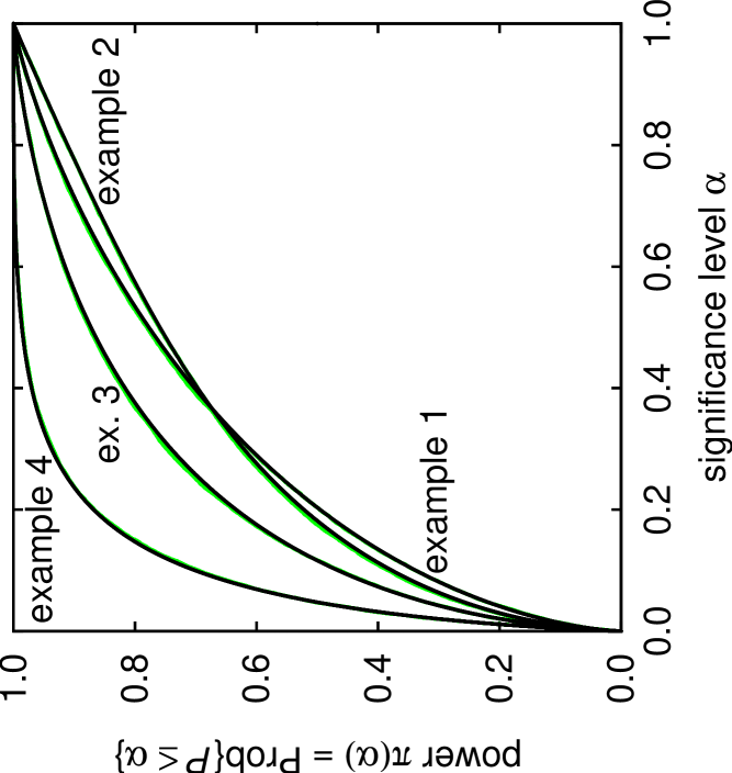
Figure 1: Cumulative distribution functions of the P-values $P$ for draws from the alternative distributions defined in Subsections 6.1–6.4

Table 1: Computational costs

	$m$	$q_{0}$	$q_{a}$	$t$
example 1	10	230	230	0.006
example 2	100	530	550	0.090
example 3	20	250	330	0.013
example 4	20	350	350	0.010

References

- Davies (1980) {barticle}[author] \bauthor\bsnmDavies, \bfnmRobert B.\binitsR. B. (\byear1980). \btitleAlgorithm AS 155: The distribution of a linear combination of random variables. \bjournalJ. Roy. Statist. Soc. Ser. C \bvolume29 \bpages323–333. \endbibitem
- Duchesne and de Micheaux (2010) {barticle}[author] \bauthor\bsnmDuchesne, \bfnmPierre\binitsP. and \bauthor\bsnmde Micheaux, \bfnmPierre Lafaye\binitsP. L. (\byear2010). \btitleComputing the distribution of quadratic forms: Further comparisons between the Liu-Tang-Zhang approximation and exact methods. \bjournalComput. Statist. Data Anal. \bvolume54 \bpages858–862. \endbibitem
- Golub and Van Loan (1996) {bbook}[author] \bauthor\bsnmGolub, \bfnmGene H.\binitsG. H. and \bauthor\bsnmVan Loan, \bfnmCharles F.\binitsC. F. (\byear1996). \btitleMatrix Computations, \bedition3rd ed. \bpublisherJohns Hopkins University Press, \baddressBaltimore, Maryland. \endbibitem
- Gu and Eisenstat (1994) {barticle}[author] \bauthor\bsnmGu, \bfnmMing\binitsM. and \bauthor\bsnmEisenstat, \bfnmStanley C.\binitsS. C. (\byear1994). \btitleA stable and efficient algorithm for the rank-one modification of the symmetric eigenproblem. \bjournalSIAM J. Matrix Anal. Appl. \bvolume15 \bpages1266–1276. \endbibitem
- Gu and Eisenstat (1995) {barticle}[author] \bauthor\bsnmGu, \bfnmMing\binitsM. and \bauthor\bsnmEisenstat, \bfnmStanley C.\binitsS. C. (\byear1995). \btitleA divide-and-conquer algorithm for the symmetric tridiagonal eigenproblem. \bjournalSIAM J. Matrix Anal. Appl. \bvolume16 \bpages172–191. \endbibitem
- Imhof (1961) {barticle}[author] \bauthor\bsnmImhof, \bfnmJ. P.\binitsJ. P. (\byear1961). \btitleComputing the distribution of quadratic forms in normal variables. \bjournalBiometrika \bvolume48 \bpages419–426. \endbibitem
- Kendall et al. (2009) {bbook}[author] \bauthor\bsnmKendall, \bfnmMaurice G.\binitsM. G., \bauthor\bsnmStuart, \bfnmAlan\binitsA., \bauthor\bsnmOrd, \bfnmKeith\binitsK. and \bauthor\bsnmArnold, \bfnmSteven\binitsS. (\byear2009). \btitleKendall’s Advanced Theory of Statistics \bvolume2A, \bedition6th ed. \bpublisherWiley. \endbibitem
- Moore and Spruill (1975) {barticle}[author] \bauthor\bsnmMoore, \bfnmDavid S.\binitsD. S. and \bauthor\bsnmSpruill, \bfnmM. C.\binitsM. C. (\byear1975). \btitleUnified large-sample theory of general chi-squared statistics for tests of fit. \bjournalAnn. Statist. \bvolume3 \bpages599–616. \endbibitem
- Perkins, Tygert, and Ward (2011a) {btechreport}[author] \bauthor\bsnmPerkins, \bfnmWilliam\binitsW., \bauthor\bsnmTygert, \bfnmMark\binitsM. and \bauthor\bsnmWard, \bfnmRachel\binitsR. (\byear2011a). \btitle and classical exact tests often wildly misreport significance; the remedy lies in computers. \btypeTechnical Report No. \bnumber1108.4126, \binstitutionarXiv. \bnotehttp://cims.nyu.edu/tygert/abbreviated.pdf. \endbibitem
- Perkins, Tygert, and Ward (2011b) {barticle}[author] \bauthor\bsnmPerkins, \bfnmWilliam\binitsW., \bauthor\bsnmTygert, \bfnmMark\binitsM. and \bauthor\bsnmWard, \bfnmRachel\binitsR. (\byear2011b). \btitleComputing the confidence levels for a root-mean-square test of goodness-of-fit. \bjournalAppl. Math. Comput. \bvolume217 \bpages9072–9084. \endbibitem
- Perkins, Tygert, and Ward (2011c) {btechreport}[author] \bauthor\bsnmPerkins, \bfnmWilliam\binitsW., \bauthor\bsnmTygert, \bfnmMark\binitsM. and \bauthor\bsnmWard, \bfnmRachel\binitsR. (\byear2011c). \btitleComputing the confidence levels for a root-mean-square test of goodness-of-fit, II \btypeTechnical Report No. \bnumber1009.2260, \binstitutionarXiv. \endbibitem
- Press et al. (2007) {bbook}[author] \bauthor\bsnmPress, \bfnmWilliam\binitsW., \bauthor\bsnmTeukolsky, \bfnmSaul\binitsS., \bauthor\bsnmVetterling, \bfnmWilliam\binitsW. and \bauthor\bsnmFlannery, \bfnmBrian\binitsB. (\byear2007). \btitleNumerical Recipes, \bedition3rd ed. \bpublisherCambridge University Press, \baddressCambridge, UK. \endbibitem
- Rao (2002) {bincollection}[author] \bauthor\bsnmRao, \bfnmCalyampudi R.\binitsC. R. (\byear2002). \btitleKarl Pearson chi-square test: The dawn of statistical inference. In \bbooktitleGoodness-of-Fit Tests and Model Validity (\beditor\bfnmC.\binitsC. \bsnmHuber-Carol, \beditor\bfnmN.\binitsN. \bsnmBalakrishnan, \beditor\bfnmM. S.\binitsM. S. \bsnmNikulin and \beditor\bfnmM.\binitsM. \bsnmMesbah, eds.) \bpages9–24. \bpublisherBirkhäuser, \baddressBoston. \endbibitem
- Rice (1980) {barticle}[author] \bauthor\bsnmRice, \bfnmStephen O.\binitsS. O. (\byear1980). \btitleDistribution of quadratic forms in normal random variables — Evaluation by numerical integration. \bjournalSIAM J. Sci. Stat. Comput. \bvolume1 \bpages438–448. \endbibitem