In the extremal Kerr spacetime the horizon Killing vector field is null on a timelike hypersurface crossing the horizon at a fixed latitude, and spacelike on both sides of the horizon in the equatorial plane. We explain in some detail how this behaviour is consistent with the existence of timelike Killing vectors everywhere off the horizon, and how it arises in a limit from the Kerr spacetime where there is a similar hypersurface strictly outside the horizon.

1. Introduction

The Kerr solution is one of the most important exact solutions ever obtained in physics, and has been thoroughly studied [1]. Its event horizon is ruled by a Killing vector field whose causal character changes from timelike to spacelike across the horizon. This is the horizon Killing field. The difference from a static black hole is that the horizon Killing field becomes null also on a timelike hypersurface surrounding the horizon. Still the existence of a Killing vector field which is timelike in a region around the event horizon is important for instance in setting up curved spacetime quantum field theory there [2].

A special case of the Kerr solution is its extremal limit, which has attracted attention recently for reasons that have more to do with quantum gravity than with astrophysics [3]. Its event horizon is again ruled by a horizon Killing field, but this Killing field becomes null on a timelike hypersurface crossing the horizon at some fixed latitude. In the equatorial plane one finds that the horizon Killing vector field is spacelike except at the horizon itself [4, 5]. This behaviour is very different from that encountered in non-extreme Kerr, and also in the spherically symmetric extremal black holes that we are familiar with. We found it puzzling. Given that the exterior of the extremal Kerr black hole is stationary, what is the Killing vector field that is timelike all the way down to the horizon? And how can we understand the behaviour of the timelike hypersurface where the horizon Killing field goes null as a limiting case of the corresponding hypersurface in the non-extreme Kerr black hole?

It turns out that the first question is posed incorrectly. We will rephrase it, and then give its answer, in section 2. The second question is not obviously well posed since the notion of limits of spacetimes is a subtle one [6]. Nevertheless it has a simple and intuitively appealing answer, that we give in section 3. Section 4 contains some comments on the near horizon geometry of extremal Kerr. In section 5 we state our conclusions.

Before we begin, we remind the reader that the Kerr metric in Boyer-Lindquist coordinates is

$$ds^{2}=-\frac{\Delta-a^{2}\sin^{2}{\theta}}{\rho^{2}}dt^{2}-\frac{4mar\sin^{2}{\theta}}{\rho^{2}}dtd\phi+\frac{\rho^{2}}{\Delta}dr^{2}+\rho^{2}d\theta^{2}+\frac{A\sin^{2}{\theta}}{\rho^{2}}d\phi^{2}\ ,$$ (1)

where

$$\rho^{2}\equiv r^{2}+a^{2}\cos^{2}{\theta}\ ,\hskip 28.45274ptA\equiv(r^{2}+a^{2})^{2}-a^{2}\Delta\sin^{2}{\theta}\ ,$$ (2)

$$\Delta\equiv r^{2}-2mr+a^{2}=(r-r_{+})(r-r_{-})\ ,\hskip 17.07164ptr_{\pm}=m\pm\sqrt{m^{2}-a^{2}}\ .$$ (3)

This coordinate system divides the Kerr spacetime into three regions:

$$\mbox{I}:\ r_{+}<r<\infty\ ,\hskip 17.07164pt\mbox{II}:\ r_{-}<r<r_{+}\ ,\hskip 17.07164pt\mbox{III}:-\infty<r<r_{-}\ .$$ (4)

Region I is the physically relevant exterior, region II lies between the two Killing horizons at $\Delta=0$, and region III contains an unphysical asymptotic region. The mass of the black hole is $m$, its angular momentum $J=am$, and its event horizon is at $r=r_{+}$. The extremal case is obtained by setting $a=m$, in which case there is no region II since the two horizons coincide. The $a<m$ case is believed to describe actually existing black holes (in the approximation that these can be regarded as isolated), while the case $a>m$ is a nakedly singular spacetime.

A general Killing vector field of the Kerr solution (whether extremal or not) is given by a linear combination

$$\xi=\partial_{t}+b\partial_{\phi}\ ,$$ (5)

where $b$ is a constant. Its norm is

$$||\partial_{t}+b\partial_{\phi}||^{2}=\frac{1}{\rho^{2}}\left[-\Delta+\sin^{2}{\theta}(a^{2}-4marb+Ab^{2})\right]\ .$$ (6)

This can vanish for all $\theta$ only if $\Delta=0$, that is on one of the horizons. It vanishes on the outer horizon $r=r_{+}$ if and only if

$$b=\frac{a}{2mr_{+}}\ .$$ (7)

This particular linear combination defines the horizon Killing vector field $\xi_{\rm hor}$. One finds indeed

$$||\xi_{\rm hor}||^{2}=-\frac{r-r_{+}}{4m^{2}\rho^{2}r_{+}^{2}}f\ ,$$ (8)

where

$$f=f(r,\theta)=-4m^{2}a^{2}\sin^{2}{\theta}(r-r_{+})+\hskip 113.81102pt$$

(9)

$$+\left(4m^{2}r_{+}^{2}-a^{2}(r^{2}+2mr+a^{2})\sin^{2}{\theta}+a^{4}\sin^{4}{\theta}\right)(r-r_{-})\ .$$

We will soon analyze these expressions in detail.

2. Timelike Killing vector fields in extreme Kerr

In the extreme case $m=a=r_{+}=r_{-}$ the expression for the norm of the horizon Killing field is easily factorized:

$$||\xi_{\rm hor}||^{2}=-\frac{(r-m)^{2}}{4m^{2}\rho^{2}}f_{1}f_{2}\ ,$$ (10)

$$f_{1}=\left(m\sin^{2}{\theta}+(r+m)\sin{\theta}-2m\right)\ ,$$ (11)

$$f_{2}=\left(m\sin^{2}{\theta}-(r+m)\sin{\theta}-2m\right)\ .$$ (12)

There is a double root at the horizon ($r=m$). The other roots describe two timelike hypersurfaces where the horizon Killing field is null, one of them at negative values of $r$. We are interested in the root defined by $f_{2}=0$. This describes a hypersurface crossing the horizon at

$$\sin{\theta}=\sqrt{3}-1\ ,$$ (13)

namely at $\theta\approx 47^{\circ}$.

In the equatorial plane $\theta=\pi/2$ the horizon Killing field is spacelike on both sides of the horizon. Still there must be timelike Killing vectors there. This is made obvious by studying the Killing bivector

$$K^{ab}=\partial_{t}^{a}\partial_{\phi}^{b}-\partial_{t}^{b}\partial_{\phi}^{a}\ .$$ (14)

Its norm is

$$\frac{1}{2}K_{ab}K^{ab}=-\Delta\sin^{2}{\theta}\ .$$ (15)

We see that the Killing vectors span a timelike 2-plane everywhere, except on the horizon ($\Delta=0$) and on the axes ($\sin{\theta}=0$). Another way of making this obvious is to observe that the Bardeen vector field, which describes the motion of a zero angular momentum observer, is timelike outside the horizon. At each point this vector field is a linear combination of the Killing vectors. See exercise 33.3 in ref. [7]. But the Bardeen vector field is not in itself a Killing vector field, since the linear combination is spacetime dependent. Also it would seem that a Killing vector field that is timelike just outside the horizon must be null on the horizon, and the horizon vector field—which is spacelike outside the horizon at least on the equatorial plane—is the only Killing vector field that does become null on the horizon. So how can there be a Killing vector field which is timelike in a region just outside the horizon?

The resolution turns out to be that there is no such Killing vector field. Nevertheless there are timelike Killing vectors at all points off the horizon. To simplify the calculations let us study the situation in the equatorial plane $\theta=\pi/2$ where the norm of a general Killing vector field is

$$||\partial_{t}+b\partial_{\phi}||^{2}=\frac{1}{r}\left[-r+2m-4m^{2}b+b^{2}(r^{3}+m^{2}r+2m^{3})\right]\ .$$ (16)

We will set $m=1$ for simplicity. Then one finds that the norm vanishes if

$$b=\frac{2\pm r(r-1)}{r^{3}+r+2}=\left\{\begin{array}[]{l}b_{+}=\frac{1}{r+1}\\ \\ b_{-}=\frac{2-r}{r^{2}-r+2}\ ,\end{array}\right.$$ (17)

It is however more interesting to see where a Killing field with a fixed value of $b$ is null. If $b=0$ this happens at $r=2$. This is where the ergosphere intersects the equatorial plane. If $b\neq 0$ we find that the norm vanishes if and only if

$$r^{3}+\frac{b^{2}-1}{b^{2}}r+\frac{2(b-1)^{2}}{b^{2}}=0\ .$$ (18)

The latter polynomial has three roots,

$$r=\frac{1-b}{b}$$ (19)

$$r=\frac{1}{2b}\left(b-1\pm\sqrt{(1-b)(7b+1)}\right)\ .$$ (20)

However, we are interested only in real roots, and primarily in positive real roots. We therefore confine ourselves to $b$ lying between $-1/7$ and $+1$. The result is shown in Fig. 1.

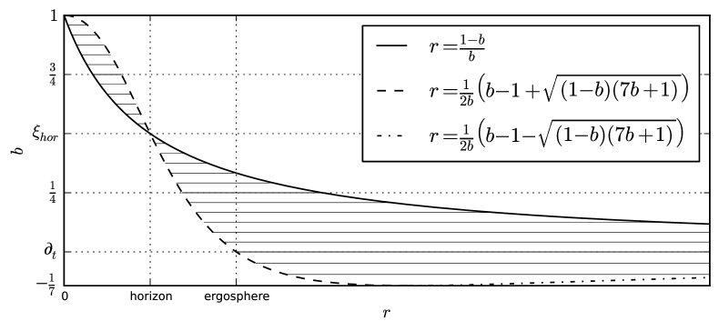
Figure 1: This picture shows the region of the equatorial plane where a given Killing vector field $\partial_{t}+b\partial_{\phi}$ is timelike, for various values of $b$.

For $b=1/2$ (the horizon Killing field) the only real root is at $r=1$, that is at the horizon itself. For smaller values of $b$ there is an annulus in the equatorial plane where the Killing vector field is timelike. For larger values of $b$ this annulus lies inside the horizon. There is one special Killing vector field, namely $\partial_{t}$, which becomes timelike at $r=2$ (the ergosphere) and “escapes” to infinity while staying timelike all the way out. For our purposes the point is that although every point in the equatorial plane belongs to one of the annuli, none of them actually extend all the way to the horizon. This is the answer to our first question.

3. The velocity-of-light surface

The timelike hypersurface where the horizon vector field goes null is called the velocity-of-light surface in ref. [5]. Possibly this is an unfortunate terminology (since other hypersurfaces go under the same name), but we will adopt it here. To understand its limiting behaviour as $a\rightarrow m$ we have to analyze the full Kerr case. Going back to eqs. (8-9), we observe that the horizon Killing field is null both at the horizon ($r=r_{+}$) and at the hypersurfaces defined by $f=f(r,\theta)=0$. Such a hypersurface can be described either as a function $r=r(\theta)$ or as a function $\theta=\theta(r)$. Indeed one finds

$$\sin{\theta}=\sqrt{\frac{h-\sqrt{h^{2}-g}}{2a^{2}\Delta}}\ ,$$ (21)

where

$$h=(r^{2}+a^{2})^{2}-4m^{2}\left(a^{2}+2r_{+}(r-m)\right)\ ,$$ (22)

$$g=16m^{2}\Delta^{2}(2mr_{+}-a^{2})\ .$$ (23)

To solve for $r$ we must find the roots of a third order polynomial. This can be done using Mathematica, but the explicit expressions do not look pleasant. Still we did use numerical solutions for $r$ in constructing our plots.

In Fig. 2 we show the results in the $r$-$\theta$-plane. The left hand column treats $r$ and $\theta$ as spanning a plane, and we see three velocity-of-light surfaces. The right hand column treats $r$ and $\theta$ as polar coordinates. This has some intuitive appeal, but it misses the admittedly unphysical region with negative values of $r$. Three different values of $a/m$ are illustrated. From the top down they are $a/m=\sqrt{2(\sqrt{2}-1)}\approx 0.91$, which is the value of the parameter for which the velocity-of-light surface touches the ergosphere, $a/m=0.999$, and $a/m=1$, which is the extremal case. The outer pair of velocity-of-light surfaces always touch a horizon at the poles. One velocity-of-light surface always touches the singularity, which sits at $(r,\theta)=(0,\pi/2)$. In the plots we have set $m=1$, the outer and inner horizons are red, the ergosphere is green, and the velocity-of-light surfaces are blue.

In Fig. 3 we see clearly how two velocity-of-light surfaces in the Kerr solution merge and form a single hypersurface crossing the horizon in the limit as $a/m$ tends to 1. This is the answer to our second question.

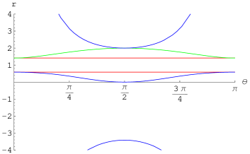
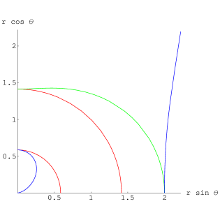
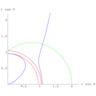
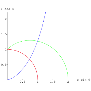
Figure 2: The velocity-of-light surfaces for different values of $\frac{a}{m}$. See the text for explanations.

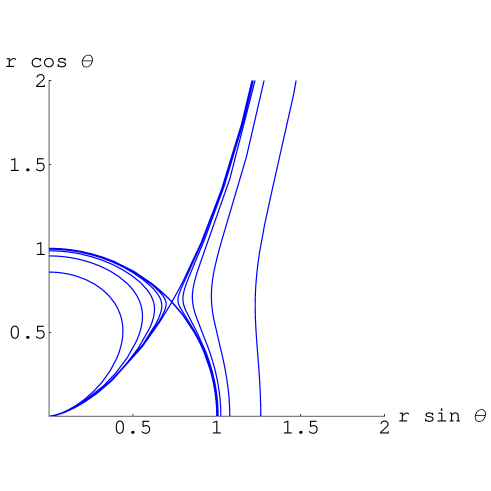
Figure 3: The velocity-of-light surfaces for $m=1$ and six different values of $a/m$: 0.99, 0.999, 0.9999, 0.99999, 0.999999, and 1, together with the event horizon of the extremal black hole.

4. The near horizon geometry

For the extremal black hole there is only one velocity-of-light surface, and it has such a simple description that we are able to report its intrinsic curvature. In particular, let $R$ be its scalar curvature and $S_{ab}=R_{ab}-1/3g_{ab}$ the traceless part of its Ricci tensor. Using CLASSI [8] to perform the calculation we obtain

$$R=-\frac{s^{3}(s+1)(12s^{8}-86s^{6}-51s^{5}+96s^{4}+44s^{3}+72s^{2}-12s-32)}{m^{2}(s^{2}-2)^{3}(4s^{3}-3s^{2}-2)^{2}}$$ (24)

$$S_{ab}S^{ab}=\frac{s^{6}(s+1)^{2}(s^{2}+2s-2)^{2}(3s^{2}-2s-2)^{2}(5s^{3}+12s^{2}+6s+8)^{2}}{24m^{2}(s^{2}-2)^{6}(4s^{3}-3s^{2}-2)^{4}}$$ (25)

where $s\equiv\sin{\theta}$. The interesting thing is that at the point where this hypersurface crosses the horizon the latter quantity, and indeed the traceless Ricci scalar itself, vanishes:

$$s=\sqrt{3}-1\hskip 14.22636pt\Rightarrow\hskip 14.22636ptS_{ab}S^{ab}=0\ .$$ (26)

There is a reason for this, as we will now explain.

In many applications [3] the near horizon limit of extremal black holes is of interest. Since this is not really our topic here we refer to the literature for the details in the Kerr case [9]. The event horizon of the extremal black hole becomes a Killing horizon in the near horizon geometry, and the horizon Killing vector field is again null on a timelike hypersurface crossing this Killing horizon at a fixed latitude. Now it happens that a timelike hypersurface at fixed latitude $\theta$ in the near horizon geometry is in itself a 2+1 dimensional spacetime of considerable interest [10]. At high latitudes it is an anti-de Sitter space squashed along a spacelike fibre (along which it has also been made periodic). At low latitudes it is stretched along the same fibres. The Killing field that generates the horizon goes null also at latitude $\theta=\arcsin{(\sqrt{3}-1)}$. This hypersurface forms the boundary between squashing and stretching, and has the intrinsic geometry of a 2+1 dimensional anti-de Sitter space. This explains the result (26).

5. Conclusions

The behaviour of the timelike Killing vector fields gives the extremal Kerr black hole an onion-like structure: in the equatorial plane the event horizon is surrounded by annuli in each of which some Killing vector field is timelike. Every point outside the horizon belongs to such an annulus, but none of the annuli reach all the way down to the horizon.

The Kerr spacetime has multiple velocity-of-light surfaces where the horizon Killing field becomes null. One lies in the exterior, another lies inside the inner horizon and touches the singularity, and a third lies at negative values of $r$. As one approaches the extremal limit of the Kerr spacetime the former two merge, in such a way that the extremal velocity-of-light surface crosses the horizon at a fixed latitude $\theta\approx 47^{\circ}$.

In the near horizon limit of the extremal black hole the velocity-of-light surface has the geometry of a 2+1 dimensional anti-de Sitter space (with one spacelike direction made periodic).

Acknowledgements: We thank Istvan Racz, José Senovilla, and Ted Jacobson for discussions. IB is supported by the Swedish Research Council under contract VR 621-2010-4060.

References

- [1] B. O’Neill: The Geometry of Kerr Black Holes, A K Peters, Wellesley, Massachusetts 1995.
- [2] V. P. Frolov and K. S. Thorne, Renormalized stress-energy tensor near the horizon of a slowly evolving, rotating black hole, Phys. Rev. D39 (1989) 2125.
- [3] G. Compère, The Kerr/CFT correspondence and its extensions: a comprehensive review, arXiv:1203.3561.
- [4] I. Racz, Does the third law of black hole thermodynamics really have a serious failure?, Class. Quant. Grav. 17 (2000) 4353.
- [5] A. J. Amsel, G. T. Horowitz, D. Marolf, and M. M. Roberts, No dynamics in the extremal Kerr throat, JHEP 09 (2009) 044.
- [6] R. Geroch, Limits of spacetimes, Commun. Math. Phys. 13 (1969) 180.
- [7] C. W. Misner, K. S. Thorne, and J. A. Wheeler: Gravitation, W. H. Freeman, San Francisco 1973.
- [8] J. E. Åman, manual for CLASSI: Classification Programs for Geometries in General Relativity, Department of Physics. Stockholm University, Technical Report, Provisional edition.
- [9] J. Bardeen and G. T. Horowitz, The extreme Kerr throat geometry: A vacuum analog of , Phys. Rev. D60 (1999) 104030.
- [10] I. Bengtsson and P. Sandin, Anti-de Sitter space, squashed and stretched, Class. Quant. Grav. 23 (2006) 971.