Inventory Management with Partially Observed Nonstationary Demand

Erhan Bayraktar Department of Mathematics, University of Michigan, Ann Arbor, MI 48109 erhan@umich.edu  and  Michael Ludkovski Department of Statistics and Applied Probability, University of California Santa Barbara, CA 93106-3110 ludkovski@pstat.ucsb.edu
Abstract.

We consider a continuous-time model for inventory management with Markov modulated non-stationary demands. We introduce active learning by assuming that the state of the world is unobserved and must be inferred by the manager. We also assume that demands are observed only when they are completely met. We first derive the explicit filtering equations and pass to an equivalent fully observed impulse control problem in terms of the sufficient statistics, the a posteriori probability process and the current inventory level. We then solve this equivalent formulation and directly characterize an optimal inventory policy. We also describe a computational procedure to calculate the value function and the optimal policy and present two numerical illustrations.

Key words and phrases:
Inventory management, Markov modulated Poisson process, hidden Markov model, partially observable demand, censored demand
E. Bayraktar is supported in part by the National Science Foundation, under grant DMS-0604491.

1. Introduction

Inventory management aims to control the supply ordering of a firm so that inventory costs are minimized and a maximum of customer orders are filled. These are competing objectives since low inventory stock reduces storage and ordering costs, whereas high inventory avoids stock-outs. The problem is complicated by the fact that real-life demand is never stationary and therefore the inventory policy should be non-stationary as well. A popular method of addressing this issue is to introduce a regime-switching (or Markov-modulated) demand model. The regime is meant to represent the economic environment faced by the firm and drives the parameters (frequency and size distribution) of the actual demand process. However, typically this economic environment is unknown. From a modeling perspective, this leads to a partially observed hidden Markov model for demand. Thus, the inventory manager must simultaneously learn the current environment (based on incoming order information), and adjust her inventory policy accordingly in anticipation of future orders.

The literature on inventory management with non-stationary Markovian demand originated with [29] who considered a continuous-time model where the demand levels or intensity are modulated by the state of the world, which are assumed to be observable. The discrete-time counterpart of this model was then analyzed by [28] who allowed a very general cost structure and proved a more formal verification theorem for existence and regularity of the value function and existence of an optimal feedback policy. More recent work on fully observed non-stationary demand can be found in [11].

Inventory management with partial information is a classical topic of operations research. In the simplest version as analyzed by [4, 25] and references therein, the demand distribution is unknown and must be learned by the controller. Thus, a finite-horizon discrete time parameter adaptive model is considered, so that the demand distribution is taken to be stationary and i.i.d., but with an unknown parameter. This parameter is then inferred over time using either an exponential smoothing or a Bayesian learning mechanism. In these papers the method of solution relied on the special structure of some particular cases (e.g. uniform demand level on [0,w]0𝑤[0,w], with w𝑤w unknown) where a dimension reduction is possible, so that the learning update is simplified. Even after that, the problem remains extremely computationally challenging; accordingly the focus of [25] has been on studying approximate myopic or limited look-ahead policies.

Another important strand of literature investigates the lost sales uncertainty. In that case, demand is observed only if it is completely met; instead of a back-order, unmet demand is lost. This then creates a partial information problem if demand levels are non-stationary. In particular, demand levels evolving according to a discrete-time Markov chain have been considered in the newsvendor context (completely perishable inventory) by [24, 13, 9], and in the general inventory management case by [7]. [8, 10] have analyzed the related case whereby current inventory level itself is uncertain.

The main inspiration for our model is the work of [30] who considered a version of the [28] model but under the assumption that current world state is unknown. The controller must therefore filter the present demand distribution to obtain information on the core process. [30] take a partially observed Markov decision processes (POMDP) formulation; since this is computationally challenging, they focus on empirical study of approximate schemes, in particular myopic and limited look-ahead learning policies, as well as open-loop feedback learning. A related problem of dynamic pricing with unobserved Markov-modulated demand levels has been recently considered by [3]. In that paper, the authors also work in the POMDP framework and propose a different approximation scheme based on the technique of information structure modification.

In this paper we consider a continuous-time model for inventory management with Markov modulated non-stationary demands. We take the [29] model as the starting point and introduce active learning by assuming that the state of the core process is unobserved and must be inferred by the controller. We will also assume that the demand is observed only when it is completely met, otherwise censoring occurs. Our work extends the results of [9, 7] and [30] to the continuous-review asynchronous setting. Use of continuous- rather than discrete-time model facilitates some of our analysis. It is also more realistic in medium-volume problems with many asynchronous orders (e.g. computer hardware parts, industrial commodities, etc.), especially in applications with strong business cycles where demand distribution is highly non-stationary. In a continuous-time model, the controller may adjust inventory immediately after a new order, but also between orders. This is because the controller’s beliefs about the demand environment are constantly evolving. Such qualitative distinction is not possible with discrete epochs where controls and demand observations are intrinsically paired.

Our method of solution consists of two stages. In the first stage (Section 2), we derive explicit filtering equations for the evolution of the conditional distribution of the core process. This is non-trivial in our model where censoring links the observed demand process with the chosen control strategy. We use the theory of partially observed point processes to extend earlier results of [2, 26, 5] in Proposition 2.1. The piecewise deterministic strong Markov process obtained in Proposition 2.1 allows us then to give a simplified and complete proof of the dynamic programming equations, and describe an optimal policy (see Section 3). We achieve this by leveraging the general probabilistic arguments for the impulse control of piecewise deterministic processes of [17, 15, 21] and using direct arguments to establish necessary properties of the value function. Our approach is in contrast with the POMDP and quasi-variational formulations in the aforementioned literature that make use of more analytic tools.

Our framework also leads to a different flavor for the numerical algorithm. The closed-form formulas obtained in Sections 2 and 3 permit us to give a direct and simple-to-implement computational scheme that yields a precise solution. Thus, we do not employ any of the approximate policies proposed in the literature, while maintaining a competitive computational complexity.

To summarize, our contribution is a full and integrated analysis of such incomplete information setting, including derivation of the filtering equations, characterization of an optimal policy and a computationally efficient numerical algorithm. Our results show the feasibility of using continuous-time partially observed models in inventory management problems. Moreover, our model allows for many custom formulations, including arbitrary ordering/storage/stock-out/salvage cost structures, different censoring formulations, perishable inventory and supply-size constraints.

The rest of the paper is organized as follows. In the rest of the introduction we will give an informal description of the inventory management problem we are considering. In Section 2 we make the formulation more precise and show that the original problem is equivalent to a fully observed impulse control problem described in terms of sufficient statistics. Moreover, we characterize the evolution of the paths of the sufficient statistics. In Section 3 we show that the value function is the unique fixed point of a functional operator (defined in terms of an optimal stopping problem) and that it is continuous in all of its variables. Using the continuity of the value function we describe an optimal policy in Section 3.2. In Section 3.3 we describe how to compute the value function using an alternative characterization. Finally, in Section 4 we present two numerical illustrations. Some of the longer proofs are left to the Appendix.

1.1. Model Description

In this section we give an informal description of the inventory management with partial information and the objective of the controller. A rigorous construction is in Section 2.

Let M𝑀M be the unobservable Markov core process for the economic environment. We assume that M𝑀M is a continuous-time Markov chain with finite state space E{1,,m}𝐸1𝑚E\triangleq\{1,\ldots,m\}. The core process M𝑀M modulates customer orders modeled as a compound Poisson process X𝑋X. More precisely, let Y1,Y2,subscript𝑌1subscript𝑌2Y_{1},Y_{2},\ldots be the consecutive order sizes, taking place at times σ1,σ2,subscript𝜎1subscript𝜎2\sigma_{1},\sigma_{2},\ldots. Define

(1.1) N(t)𝑁𝑡\displaystyle N(t) =sup{s:σs<t}absentsupremumconditional-set𝑠subscript𝜎𝑠𝑡\displaystyle=\sup\{s:\sigma_{s}<t\}

to be the number of orders received by time t𝑡t, and

(1.2) Xt=k=1N(t)Yk,subscript𝑋𝑡superscriptsubscript𝑘1𝑁𝑡subscript𝑌𝑘\displaystyle X_{t}=\sum_{k=1}^{N(t)}Y_{k},

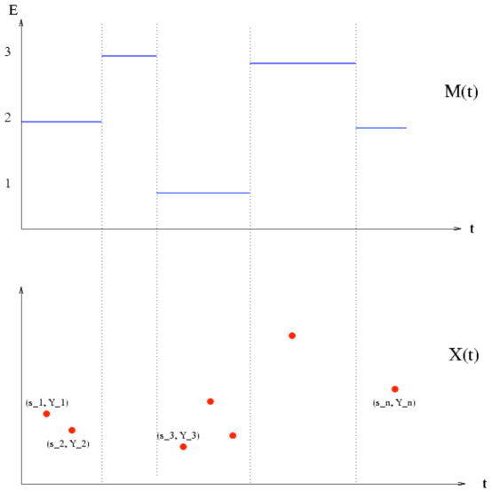
to be the total order size by time t𝑡t. Then, the intensity of N𝑁N (and X𝑋X) is λisubscript𝜆𝑖\lambda_{i} whenever M𝑀M is at state i𝑖i, for iE𝑖𝐸i\in E. Similarly, the distribution of Yksubscript𝑌𝑘Y_{k} is νisubscript𝜈𝑖\nu_{i} conditional on Mσk=isubscript𝑀subscript𝜎𝑘𝑖M_{\sigma_{k}}=i. This structure is illustrated schematically in Figure 1. The assumption of demand following a compound Poisson process is standard in the OR literature, especially when considering large items (the case of demand level following a jump-diffusion is investigated by [11]).
Refer to caption
Figure 1. The environment process M𝑀M modulates the marked point process X=((σ1,Y1),)𝑋subscript𝜎1subscript𝑌1X=((\sigma_{1},Y_{1}),\ldots) representing demand order flow. In this illustration, M𝑀M takes the values Mt{1,2,3}=Esubscript𝑀𝑡123𝐸M_{t}\in\{1,2,3\}=E, and the mark distributions are arranged such that μ1<μ2<μ3subscript𝜇1subscript𝜇2subscript𝜇3\mu_{1}<\mu_{2}<\mu_{3} where μi=𝔼[Y|Mt=i]subscript𝜇𝑖𝔼delimited-[]conditional𝑌subscript𝑀𝑡𝑖\mu_{i}=\mathbb{E}[Y|M_{t}=i]. Also, the intensities are arranged λ3<λ2<λ1subscript𝜆3subscript𝜆2subscript𝜆1\lambda_{3}<\lambda_{2}<\lambda_{1}, with λi=𝔼[σ1|Mu=i,0uT]subscript𝜆𝑖𝔼delimited-[]formulae-sequenceconditionalsubscript𝜎1subscript𝑀𝑢𝑖0𝑢𝑇\lambda_{i}=\mathbb{E}[\sigma_{1}|M_{u}=i,0\leq u\leq T]. Thus, in regime 1 demand is frequent and demand amounts are small, in regime 2 demand is average and amounts are small to average, and in regime 3 demand is rare but consists of relatively large orders.

We assume that orders are integer-sized with a fixed upper bound R𝑅R, namely

Assumption.

Each νisubscript𝜈𝑖\nu_{i}, iE𝑖𝐸i\in E is a discrete bounded distribution on \mathbb{Z}, so that Yk{1,2,,R}subscript𝑌𝑘12𝑅Y_{k}\in\{1,2,\ldots,R\}.

The controller cannot observe M𝑀M; neither does she directly see X𝑋X. Instead, she receives the censored order flow W𝑊W. The order flow W𝑊W consists of filled order amounts (Z)subscript𝑍(Z_{\ell}), which informally correspond to the minimum between actual order size and available inventory. Hence, if total inventory is insufficient, a stock-out occurs and the excess order size is left indeterminate. The model where order flow is always observed will also be considered as a special case with zero censoring. The precise description of W𝑊W will be given in Section 2.1.

Let Ptsubscript𝑃𝑡P_{t} be the current inventory at time t𝑡t. We assume that inventory has finite stock capacity, so that Pt[0,P¯]subscript𝑃𝑡0¯𝑃P_{t}\in[0,\overline{P}]. Inventory changes are driven by two variables: filled customer orders described by W𝑊W and supply orders. Customer orders are assumed to be exogenous; every order is immediately filled to its maximum extent. When a stock-out occurs, we consider two scenarios:

  • If there is no censoring, then the excess order amount is immediately back-ordered at a higher penalty rate.

  • If there is censoring, a lost opportunity cost is assessed in proportion to expected excess order amount.

Otherwise, the inventory is immediately decreased by the order amount. Supply orders are completely at the discretion of the manager. Let ξ1,ξ2,subscript𝜉1subscript𝜉2\xi_{1},\xi_{2},\ldots denote the supply amounts (without back-orders) and τ1,τ2,subscript𝜏1subscript𝜏2\tau_{1},\tau_{2},\ldots the supply times (when supply order is placed).

To summarize, the dynamics of P𝑃P are (compare to (2.12) below):

(1.6) {Pσk=(PσkZk),fill customer orderPτk=Pτk+ξk,new supply orderdPt=0otherwise.casessubscript𝑃subscript𝜎𝑘absentsubscript𝑃limit-fromsubscript𝜎𝑘subscript𝑍𝑘fill customer ordersubscript𝑃subscript𝜏𝑘absentsubscript𝑃limit-fromsubscript𝜏𝑘subscript𝜉𝑘new supply order𝑑subscript𝑃𝑡absent0otherwise\displaystyle\left\{\begin{array}[]{lrr}P_{\sigma_{k}}&=(P_{\sigma_{k}-}-Z_{k}),&\text{fill customer order}\\ P_{\tau_{k}}&=P_{\tau_{k}-}+\xi_{k},&\text{new supply order}\\ dP_{t}&=0&\text{otherwise}.\end{array}\right.

We assume that the manager can only increase inventory (no disposal is possible) and that inventory never perishes. Alternatives can be straightforwardly dealt with and are considered in a numerical example in Section 3.3.

We denote the entire inventory strategy by the right-continuous piecewise constant process ξ:[0,T]×Ω𝒜:𝜉0𝑇Ω𝒜\xi\colon[0,T]\times\Omega\to\mathcal{A}, with ξt=ξksubscript𝜉𝑡subscript𝜉𝑘\xi_{t}=\xi_{k} if τkt<τk+1subscript𝜏𝑘𝑡subscript𝜏𝑘1\tau_{k}\leqslant t<\tau_{k+1} or

(1.7) ξt=τkTξk1[τk,τk+1)(t).subscript𝜉𝑡subscriptsubscript𝜏𝑘𝑇subscript𝜉𝑘subscript1subscript𝜏𝑘subscript𝜏𝑘1𝑡\displaystyle\xi_{t}=\sum_{\tau_{k}\leq T}\xi_{k}\cdot 1_{[\tau_{k},\tau_{k+1})}(t).

The goal of the inventory manager is to minimize inventory costs as appearing in the objective function (1.8) below among all admissible inventory strategies ξ𝜉\xi. The admissibility condition concerns first and foremost the information set available to the manager. Because only W𝑊W is observable, the strategy ξ𝜉\xi should be determined by the information generated by W𝑊W, namely each τksubscript𝜏𝑘\tau_{k} must be a stopping time of the filtration 𝔽W{tW}superscript𝔽𝑊subscriptsuperscript𝑊𝑡\mathbb{F}^{W}\triangleq\{\mathcal{F}^{W}_{t}\} of W𝑊W. Similarly, the value of each ξksubscript𝜉𝑘\xi_{k} is determined by the information τkWsubscriptsuperscript𝑊subscript𝜏𝑘\mathcal{F}^{W}_{\tau_{k}} revealed by W𝑊W until τksubscript𝜏𝑘\tau_{k}. Also, without loss of generality we assume that ξ𝜉\xi has a finite number of actions, so that (τk<T)0subscript𝜏𝑘𝑇0\mathbb{P}(\tau_{k}<T)\to 0 as k𝑘k\to\infty. Since strategies with infinitely many actions will have infinite costs, we can safely exclude them from consideration. We denote by 𝒰(T)𝒰𝑇\mathcal{U}(T) the set of all such admissible strategies on a time interval [0,T]0𝑇[0,T].

The selected policy ξ𝜉\xi directly influences current stocks P𝑃P; when we wish to emphasize this dependence we will write PtPtξsubscript𝑃𝑡superscriptsubscript𝑃𝑡𝜉P_{t}\equiv P_{t}^{\xi}. The cost of implementing ξ𝜉\xi is as follows. First, inventory storage costs at fixed rate c(Pt)𝑐subscript𝑃𝑡c(P_{t}) are accessed. We assume that c𝑐c is positive, increasing and continuous. Second, a supply order of size ξksubscript𝜉𝑘\xi_{k} costs hξk+ζsubscript𝜉𝑘𝜁h\cdot\xi_{k}+\zeta, for positive hh and ζ𝜁\zeta. Finally, if a stock-out occurs due to insufficient existing stock, a penalty reflecting the lost opportunity cost is assessed at amount 𝔼[K((YkPσk)+)|tW]𝔼delimited-[]conditional𝐾subscriptsubscript𝑌𝑘subscript𝑃limit-fromsubscript𝜎𝑘subscriptsuperscript𝑊𝑡\mathbb{E}\left[K((Y_{k}-P_{\sigma_{k}-})_{+})|\mathcal{F}^{W}_{t}\right]. We assume that the penalty function K𝐾K is positive and increasing with K(0)=0𝐾00K(0)=0. Thus, the total performance of a strategy ξ𝜉\xi on the horizon [0,T]0𝑇[0,T] is

(1.8) 0Teρtc(Pt)𝑑t+k:τk<Teρτk(hξk+ζ)+:σ<TeρσK((YPσ)+),superscriptsubscript0𝑇superscripte𝜌𝑡𝑐subscript𝑃𝑡differential-d𝑡subscript:𝑘subscript𝜏𝑘𝑇superscripte𝜌subscript𝜏𝑘subscript𝜉𝑘𝜁subscript:subscript𝜎𝑇superscripte𝜌subscript𝜎𝐾subscriptsubscript𝑌subscript𝑃limit-fromsubscript𝜎\displaystyle\int_{0}^{T}\mathrm{e}^{-\rho t}c(P_{t})\,dt+\sum_{k:\tau_{k}<T}\mathrm{e}^{-\rho\tau_{k}}(h\cdot\xi_{k}+\zeta)+\sum_{\ell:\sigma_{\ell}<T}\mathrm{e}^{-\rho\sigma_{\ell}}K((Y_{\ell}-P_{\sigma_{\ell}-})_{+}),

where ρ0𝜌0\rho\geq 0 is the discount factor for future revenue. Table 1 summarizes our notation and the meaning of the model parameters.

Parameter Meaning
c(a)𝑐𝑎c(a) storage cost for a𝑎a items per unit time
K(a)𝐾𝑎K(a) instantaneous stock-out cost for a shortage of a𝑎a items
hh order cost for one item
ζ𝜁\zeta fixed cost of placing an order
ρ𝜌\rho discount factor for NPV calculation
P¯¯𝑃\overline{P} maximum inventory size
R𝑅R maximum demand size
Table 1. Parameters of the model

Observe that the objective in (1.8) involves the distribution of Zksubscript𝑍𝑘Z_{k}’s (which affect P𝑃P) and Yksubscript𝑌𝑘Y_{k}’s (which enter into objective function through stock-out costs). Both of these depend on the state M𝑀M. Since the core process M𝑀M is unobserved, the controller must therefore carry out a filtering procedure. We postulate that she collects information about M𝑀M via a Bayesian framework. Let π=(π1,,πm)({M0=1},,{M0=m})𝜋subscript𝜋1subscript𝜋𝑚subscript𝑀01subscript𝑀0𝑚\vec{\pi}=(\pi_{1},\ldots,\pi_{m})\triangleq\left(\mathbb{P}\{M_{0}=1\},\ldots,\mathbb{P}\{M_{0}=m\}\right) be the initial (prior) beliefs of the controller about M𝑀M and πsuperscript𝜋\mathbb{P}^{\vec{\pi}} the corresponding conditional probability law. The controller starts with beliefs π𝜋\pi, observes Z𝑍Z, updates her beliefs and adjusts her inventory policy accordingly.

These notions and the precise updating mechanism will be formalized in Section 2.4. The solution will then proceed in two steps: an initial filtering step and a second optimization step. The inference step is studied in Section 2, where we introduce the a posteriori probability process ΠΠ\vec{\Pi}. The process ΠΠ\vec{\Pi} summarizes the dynamic updating of controller’s beliefs about the Markov chain M𝑀M given her point process observations. The optimal switching problem (2.5) is then analyzed in Section 3.

2. Problem Statement

In this section we give a mathematically precise description of the problem and show that this problem is equivalent to a fully observed impulse control problem in terms of the strong Markov process (Π,P)Π𝑃(\vec{\Pi},P). We will also describe the dynamics of the sufficient statistics (Π,P)Π𝑃(\vec{\Pi},P).

2.1. Core Process

Let (Ω,,)Ω(\Omega,\mathcal{H},\mathbb{P}) be a probability space hosting two independent elements: (i) a continuous time Markov process M𝑀M taking values in a finite set E𝐸E, and with infinitesimal generator Q=(qij)i,jE𝑄subscriptsubscript𝑞𝑖𝑗𝑖𝑗𝐸Q=(q_{ij})_{i,j\in E}, (ii) X(1),,X(m)superscript𝑋1superscript𝑋𝑚X^{(1)},\ldots,X^{(m)} which are independent compound Poisson processes with intensities and discrete jump size distributions (λ1,ν1),,(λm,νm)subscript𝜆1subscript𝜈1subscript𝜆𝑚subscript𝜈𝑚(\lambda_{1},\nu_{1}),\ldots,(\lambda_{m},\nu_{m}), respectively, mE𝑚𝐸m\in E.

The core point process X𝑋X is given by

(2.1) XtX0+0tiE1{Ms=i}dXs(i),t0.formulae-sequencesubscript𝑋𝑡subscript𝑋0superscriptsubscript0𝑡subscript𝑖𝐸subscript1subscript𝑀𝑠𝑖𝑑subscriptsuperscript𝑋𝑖𝑠𝑡0\displaystyle X_{t}\triangleq X_{0}+\int_{0}^{t}\sum_{i\in E}1_{\{M_{s}=i\}}\,dX^{(i)}_{s},\quad t\geq 0.

Thus, X𝑋X is a Markov-modulated Poisson process (see e.g. [23]); by construction, X𝑋X has independent increments conditioned on M={Mt}t0𝑀subscriptsubscript𝑀𝑡𝑡0M=\{M_{t}\}_{t\geq 0}. Denote by σ0,σ1,subscript𝜎0subscript𝜎1\sigma_{0},\sigma_{1},\ldots the arrival times of the process X𝑋X,

σinf{t>σ1:XtXt},1with σ00.formulae-sequencesubscript𝜎infimumconditional-set𝑡subscript𝜎1subscript𝑋𝑡subscript𝑋limit-from𝑡1with σ00.\displaystyle\sigma_{\ell}\triangleq\inf\{t>\sigma_{\ell-1}:X_{t}\neq X_{t-}\},\qquad\ell\geq 1\qquad\text{with $\sigma_{0}\equiv 0$.}

and by Y1,Y2,subscript𝑌1subscript𝑌2Y_{1},Y_{2},\ldots the \mathbb{R}-valued marks (demand sizes) observed at these arrival times:

Y=XσXσ,1.formulae-sequencesubscript𝑌subscript𝑋subscript𝜎subscript𝑋limit-fromsubscript𝜎1\displaystyle Y_{\ell}=X_{\sigma_{\ell}}-X_{\sigma_{\ell}-},\qquad\ell\geq 1.

Then conditioned on {Mσ=i}subscript𝑀subscript𝜎𝑖\{M_{\sigma_{\ell}}=i\}, the distribution of Ysubscript𝑌Y_{\ell} is described by νi(dy)=fi(y)dysubscript𝜈𝑖𝑑𝑦subscript𝑓𝑖𝑦𝑑𝑦\nu_{i}(dy)=f_{i}(y)dy on (+,(+))subscriptsubscript(\mathbb{Z}_{+},\mathcal{B}(\mathbb{Z}_{+})).

2.2. Observation Process

Starting with the marked point process (M,X)𝑀𝑋(M,X), the observable is a point process W𝑊W which is derived from (M,X)𝑀𝑋(M,X). This means that the marks of W𝑊W are completely determined by (M,X)𝑀𝑋(M,X) (and the control). Fix an initial stock Pˇ0(1)=asubscriptsuperscriptˇ𝑃10𝑎\check{P}^{(1)}_{0}=a. We first construct an auxiliary process Wˇ(1)superscriptˇ𝑊1\check{W}^{(1)}. The first mark of Wˇ(1)superscriptˇ𝑊1\check{W}^{(1)} is (σ1,Z1)subscript𝜎1subscript𝑍1(\sigma_{1},Z_{1}), where σ1subscript𝜎1\sigma_{1} is the first arrival time of X𝑋X and where the distribution of the first jump size Z1=(Z11,Z12)𝒵subscript𝑍1subscriptsuperscript𝑍11subscriptsuperscript𝑍21𝒵Z_{1}=(Z^{1}_{1},Z^{2}_{1})\in\mathcal{Z} conditional on (M,X)𝑀𝑋(M,X) given by

(Z1=z|Y1=y,Mσ1=i)=𝒞(y,z;Pˇσ1(1)),\mathbb{P}(Z_{1}=\vec{z}|Y_{1}=y,M_{\sigma_{1}}=i)=\mathcal{C}(y,\vec{z};{\check{P}^{(1)}_{\sigma_{1}-}}),

where 𝒞(y,z;a)𝒞𝑦𝑧𝑎\mathcal{C}(y,\vec{z};a), y+,z𝒵,a[0,P¯]formulae-sequence𝑦subscriptformulae-sequence𝑧𝒵𝑎0¯𝑃y\in\mathbb{Z}_{+},\vec{z}\in\mathcal{Z},a\in[0,\overline{P}] are the {0,1}01\{0,1\}-valued censoring functions satisfying z𝒵𝒞(y,z;a){0,1}subscript𝑧𝒵𝒞𝑦𝑧𝑎01\sum_{\vec{z}\in\mathcal{Z}}\mathcal{C}(y,\vec{z};a)\in\{0,1\}. In our context, it is convenient to take 𝒵=+×{0,Δ}𝒵subscript0Δ\mathcal{Z}=\mathbb{Z}_{+}\times\{0,\Delta\}, where z(z1,z2)𝒵𝑧superscript𝑧1superscript𝑧2𝒵\vec{z}\equiv(z^{1},z^{2})\in\mathcal{Z} represents a filled order of size z1superscript𝑧1z^{1}, and the second component z2superscript𝑧2z^{2} indicates whether a stock-out occurred or not. Censoring of excess orders then corresponds to 𝒞(y,z;p)=1{(0,p]}(y)1{(y,0)}(z)+1{(p,R)}(y)1{(p,Δ)}(z)𝒞𝑦𝑧𝑝subscript10𝑝𝑦subscript1𝑦0𝑧subscript1𝑝𝑅𝑦subscript1𝑝Δ𝑧\mathcal{C}(y,\vec{z};p)=1_{\{(0,p]\}}(y)1_{\{(y,0)\}}(\vec{z})+1_{\{(p,R)\}}(y)1_{\{(\lfloor p\rfloor,\Delta)\}}(\vec{z}). Alternatively, without censoring we take 𝒵=+×+𝒵subscriptsubscript\mathcal{Z}=\mathbb{Z}_{+}\times\mathbb{Z}_{+} (second component now indicating actual order size), and 𝒞(y,z;p)=1{(0,p]}(y)1{(y,y)}(z)+1{(p,R]}(y)1{(p,y)}(z)𝒞𝑦𝑧𝑝subscript10𝑝𝑦subscript1𝑦𝑦𝑧subscript1𝑝𝑅𝑦subscript1𝑝𝑦𝑧\mathcal{C}(y,\vec{z};p)=1_{\{(0,p]\}}(y)1_{\{(y,y)\}}(\vec{z})+1_{\{(p,R]\}}(y)1_{\{(\lfloor p\rfloor,y)\}}(\vec{z}).

Once (σ1,Z1)subscript𝜎1subscript𝑍1(\sigma_{1},Z_{1}) is observed, we update Pˇσ1(1)=aZ110subscriptsuperscriptˇ𝑃1subscript𝜎1𝑎subscriptsuperscript𝑍110\check{P}^{(1)}_{\sigma_{1}}=a-Z^{1}_{1}\geq 0, and set Pˇt(1)=Pˇσ1(1)subscriptsuperscriptˇ𝑃1𝑡subscriptsuperscriptˇ𝑃1subscript𝜎1\check{P}^{(1)}_{t}=\check{P}^{(1)}_{\sigma_{1}} for σ1t<σ2subscript𝜎1𝑡subscript𝜎2\sigma_{1}\leq t<\sigma_{2}, where σ2subscript𝜎2\sigma_{2} is the second arrival time of X𝑋X. Proceeding as before, we will obtain the marked point process Wˇ(1)=(σ,Z)superscriptˇ𝑊1subscript𝜎subscript𝑍\check{W}^{(1)}=(\sigma_{\ell},Z_{\ell}) and the corresponding uncontrolled stock process Pˇ(1)superscriptˇ𝑃1\check{P}^{(1)}.

We now introduce the first impulse control. Let {tWˇ(1)}subscriptsuperscriptsuperscriptˇ𝑊1𝑡\{\mathcal{F}^{\check{W}^{(1)}}_{t}\} be the filtration generated by Wˇ(1)superscriptˇ𝑊1\check{W}^{(1)}, and let (τ1,ξ1)subscript𝜏1subscript𝜉1(\tau_{1},\xi_{1}) be an Wˇ(1)superscriptsuperscriptˇ𝑊1\mathcal{F}^{\check{W}^{(1)}}-stopping time, and an τ1Wˇ(1)subscriptsuperscriptsuperscriptˇ𝑊1subscript𝜏1\mathcal{F}^{\check{W}^{(1)}}_{\tau_{1}}-measurable +subscript\mathbb{Z}_{+}-valued random variable, respectively, satisfying τ1T,0ξ1P¯Pˇτ1(1)formulae-sequencesubscript𝜏1𝑇0subscript𝜉1¯𝑃subscriptsuperscriptˇ𝑃1limit-fromsubscript𝜏1\tau_{1}\leq T,0\leq\xi_{1}\leq\overline{P}-\check{P}^{(1)}_{\tau_{1}-}. The impulse control means that we take W=Wˇ(1)1[0,τ1)𝑊superscriptˇ𝑊1subscript10subscript𝜏1W=\check{W}^{(1)}1_{[0,\tau_{1})}, Pt=Pˇt(1)1[0,τ1)subscript𝑃𝑡subscriptsuperscriptˇ𝑃1𝑡subscript10subscript𝜏1P_{t}=\check{P}^{(1)}_{t}1_{[0,\tau_{1})} and repeat the above construction on the interval [τ1,T]subscript𝜏1𝑇[\tau_{1},T] starting with the updated value Pˇτ1(2)=Pˇτ1(1)+ξ1subscriptsuperscriptˇ𝑃2subscript𝜏1subscriptsuperscriptˇ𝑃1limit-fromsubscript𝜏1subscript𝜉1\check{P}^{(2)}_{\tau_{1}}=\check{P}^{(1)}_{\tau_{1}-}+\xi_{1}.

Inductively this provides the auxiliary point processes Wˇ(k)superscriptˇ𝑊𝑘\check{W}^{(k)} together with the impulse controls (τk,ξk)subscript𝜏𝑘subscript𝜉𝑘(\tau_{k},\xi_{k}), k=1,2,𝑘12k=1,2,\ldots. Letting ξ=(τ1,ξ1,τ2,ξ2,)𝜉subscript𝜏1subscript𝜉1subscript𝜏2subscript𝜉2\xi=(\tau_{1},\xi_{1},\tau_{2},\xi_{2},\ldots) we finally obtain the ξ𝜉\xi-controlled inventory process P𝑃P, as well as the ξ𝜉\xi-controlled marked point process W=kWˇ(k)1[0,τk)𝑊subscript𝑘superscriptˇ𝑊𝑘subscript10subscript𝜏𝑘W=\sum_{k}\check{W}^{(k)}1_{[0,\tau_{k})}. By construction, both P𝑃P and ξ𝜉\xi are 𝔽Wsuperscript𝔽𝑊\mathbb{F}^{W}-measurable. We denote by a,ξsuperscript𝑎𝜉\mathbb{P}^{a,\xi} the resulting probability law of (W,P)𝑊𝑃(W,P).

Summarizing, P𝑃P is a piecewise-deterministic controlled process taking values in [0,P¯]0¯𝑃[0,\overline{P}] and evolving as in (1.6); the arrival times of W𝑊W are those of X𝑋X, and the distribution of its marks (Z)subscript𝑍(Z_{\ell}) depends inductively on the latest Pσsubscript𝑃limit-fromsubscript𝜎P_{\sigma_{\ell}-}, the mark Ysubscript𝑌Y_{\ell} of core process X𝑋X, and the censoring functions cip(y,z)subscriptsuperscript𝑐𝑝𝑖𝑦𝑧c^{p}_{i}(y,z). For further details of the above construction of a,ξsuperscript𝑎𝜉\mathbb{P}^{a,\xi} we refer the reader to [17, pp. 228-230]. Our use of censoring functions is similar to the construction in [2].

2.3. Statement of the Objective Function in Terms of Sufficient Statistics.

Let D{π[0,1]m:π1++πm=1}𝐷conditional-set𝜋superscript01𝑚subscript𝜋1subscript𝜋𝑚1D\triangleq\{\vec{\pi}\in[0,1]^{m}\colon\pi_{1}+\ldots+\pi_{m}=1\} be the space of prior distributions of the Markov process M𝑀M. Also, let 𝒮(s)={τ:𝔽stopping time,τs,a.s}𝒮𝑠conditional-set𝜏formulae-sequence𝔽stopping time𝜏𝑠a.s\mathcal{S}(s)=\{\tau\colon\mathbb{F}-\text{stopping time},\tau\leq s,\mathbb{P}-\text{a.s}\} denote the set of all 𝔽𝔽\mathbb{F}-stopping times smaller than or equal to s𝑠s.

Let π,a,ξsuperscript𝜋𝑎𝜉\mathbb{P}^{\vec{\pi},a,\xi} denote the probability measure a,ξsuperscript𝑎𝜉\mathbb{P}^{a,\xi} such that the process M𝑀M has initial distribution π𝜋\vec{\pi}. That is,

(2.2) π,a,ξ{A}=π1a,ξ{A|M0=1}++πna,ξ{A|M0=n}superscript𝜋𝑎𝜉𝐴subscript𝜋1superscript𝑎𝜉conditional-set𝐴subscript𝑀01subscript𝜋𝑛superscript𝑎𝜉conditional-set𝐴subscript𝑀0𝑛\mathbb{P}^{\vec{\pi},a,\xi}\{A\}=\pi_{1}\,\mathbb{P}^{a,\xi}\{A|M_{0}=1\}+\ldots+\pi_{n}\,\mathbb{P}^{a,\xi}\{A|M_{0}=n\}

for all ATW𝐴superscriptsubscript𝑇𝑊A\in\mathcal{F}_{T}^{W}. πsuperscript𝜋\mathbb{P}^{\vec{\pi}} can be similarly defined. In the sequel, when ξ0𝜉0\xi\equiv 0, we will denote the corresponding probability measure by π,asuperscript𝜋𝑎\mathbb{P}^{\vec{\pi},a}

We define the D𝐷D-valued conditional probability process Π(t)(Π1(t),,Πm(t))Π𝑡subscriptΠ1𝑡subscriptΠ𝑚𝑡\vec{\Pi}(t)\triangleq\left(\Pi_{1}(t),\ldots,\Pi_{m}(t)\right) such that

(2.3) Πi(t)=π,a,ξ{Mt=i|tW},for iE, and t0.subscriptΠ𝑖𝑡superscript𝜋𝑎𝜉conditional-setsubscript𝑀𝑡𝑖subscriptsuperscript𝑊𝑡for iE, and t0\displaystyle\Pi_{i}(t)=\mathbb{P}^{\vec{\pi},a,\xi}\{M_{t}=i|\mathcal{F}^{W}_{t}\},\quad\text{for $i\in E$, and $t\geq 0$}.

Each component of ΠΠ\vec{\Pi} gives the conditional probability that the current state of M𝑀M is {i}𝑖\{i\} given the information generated by W𝑊W until the current time t𝑡t.

Using ΠΠ\vec{\Pi} we convert the original objective (1.8) into the following 𝔽𝔽\mathbb{F}-adapted formulation. Observe that given Π(σ)Πsubscript𝜎\vec{\Pi}(\sigma_{\ell}), the distribution of Ysubscript𝑌Y_{\ell} is iEΠi(σ)νisubscript𝑖𝐸subscriptΠ𝑖limit-fromsubscript𝜎subscript𝜈𝑖\sum_{i\in E}\Pi_{i}(\sigma_{\ell}-)\nu_{i}. Therefore, starting with initial inventory a[0,P¯]𝑎0¯𝑃a\in[0,\overline{P}] and beliefs π𝜋\vec{\pi}, the performance of a given policy ξ𝒰(T)𝜉𝒰𝑇\xi\in\mathcal{U}(T) is

(2.4) Jξ(T,π,a)𝔼π,a,ξ[0Teρtc(Pt)dt++eρσiEΠi(σ)+K((yPσ)+)νi(dy)+k+eρτk(hξk+ζ)].superscript𝐽𝜉𝑇𝜋𝑎superscript𝔼𝜋𝑎𝜉delimited-[]superscriptsubscript0𝑇superscripte𝜌𝑡𝑐subscript𝑃𝑡𝑑𝑡subscriptsubscriptsuperscripte𝜌subscript𝜎subscript𝑖𝐸subscriptΠ𝑖subscript𝜎subscriptsubscript𝐾subscript𝑦subscript𝑃limit-fromsubscript𝜎subscript𝜈𝑖𝑑𝑦subscript𝑘subscriptsuperscripte𝜌subscript𝜏𝑘subscript𝜉𝑘𝜁\begin{split}J^{\xi}(T,\vec{\pi},a)&\triangleq\mathbb{E}^{\vec{\pi},a,\xi}\bigg{[}\int_{0}^{T}\mathrm{e}^{-\rho t}c(P_{t})\,dt+\sum_{\ell\in\mathbb{N}_{+}}\mathrm{e}^{-\rho\sigma_{\ell}}\sum_{i\in E}\Pi_{i}(\sigma_{\ell})\int_{\mathbb{R}_{+}}K\left((y-P_{\sigma_{\ell}-})_{+}\right)\nu_{i}(dy)\\ &\qquad+\sum_{k\in\mathbb{N}_{+}}\mathrm{e}^{-\rho\tau_{k}}(h\xi_{k}+\zeta)\bigg{]}.\end{split}

The first argument in Jξsuperscript𝐽𝜉J^{\xi} is the remaining time to maturity. Also, (2.4) assumed that the terminal salvage value is zero, so at T𝑇T the remaining inventory is completely forfeited. The inventory optimization problem is to compute

(2.5) U(T,π,a)infξ𝒰(T)Jξ(T,π,a),𝑈𝑇𝜋𝑎subscriptinfimum𝜉𝒰𝑇superscript𝐽𝜉𝑇𝜋𝑎\displaystyle U(T,\vec{\pi},a)\triangleq\inf_{\xi\in\mathcal{U}(T)}J^{\xi}(T,\vec{\pi},a),

and, if it exists, find an admissible strategy ξsuperscript𝜉\xi^{*} attaining this value. Without loss of generality we will restrict the set of admissible strategies satisfying

(2.6) 𝔼π,a,ξ[k+eρτk(hξk+ζ)]<superscript𝔼𝜋𝑎𝜉delimited-[]subscript𝑘subscriptsuperscripte𝜌subscript𝜏𝑘subscript𝜉𝑘𝜁\mathbb{E}^{\vec{\pi},a,\xi}\left[\sum_{k\in\mathbb{N}_{+}}\mathrm{e}^{-\rho\tau_{k}}(h\cdot\xi_{k}+\zeta)\right]<\infty

otherwise infinite costs would be incurred. Note that the admisible strategies have finitely many switches almost surely for any given path. The equivalence between the “separated” value function in (2.5) and the original setting of (1.8) is standard in Markovian impulse control problems, see e.g. [12].

The following notation will be used in the subsequent analysis:

(2.7) I(t)0tiEλi1{Ms=i}ds,𝐼𝑡superscriptsubscript0𝑡subscript𝑖𝐸subscript𝜆𝑖subscript1subscript𝑀𝑠𝑖𝑑𝑠I(t)\triangleq\int_{0}^{t}\sum_{i\in E}\lambda_{i}1_{\{M_{s}=i\}}ds,

and

(2.8) λ¯maxiEλi.¯𝜆subscript𝑖𝐸subscript𝜆𝑖\overline{\lambda}\triangleq\max_{i\in E}\lambda_{i}.

It is worth noting that the probability of no events for the next u𝑢u time units is π{σ1>u}=𝔼π[eI(u)]superscript𝜋subscript𝜎1𝑢superscript𝔼𝜋delimited-[]superscripte𝐼𝑢\mathbb{P}^{\vec{\pi}}\{\sigma_{1}>u\}=\mathbb{E}^{\vec{\pi}}[\mathrm{e}^{-I(u)}].

2.4. Sample paths of (Π,P)Π𝑃(\vec{\Pi},P).

In this section we describe the filtering procedure of the controller. In particular, Theorem 2.1 explicitly shows the evolution of the processes (Π,P)Π𝑃(\vec{\Pi},P). This is non-trivial in our model where censoring links the observed demand process with the chosen control strategy. The description of paths of the conditional probability process when the control does not alter the observations is discussed in Proposition 2.1 in [26] and Proposition 2.1 of [6]. Filtering with point process observations has also been studied by [2, 19, 20, 1]. Also, see [18] for general description of inference in various hidden Markov models in discrete time.

Even though the original order process X𝑋X has conditionally independent increments, this is no longer true for the observed requests W𝑊W since the censoring functions depend on P𝑃P which in turn depends on previous marks of W𝑊W. Nevertheless, given Ms=isubscript𝑀𝑠𝑖M_{s}=i for 0sσ0𝑠subscript𝜎0\leq s\leq\sigma_{\ell}, the interarrival times of W𝑊W are i.i.d. Exp(λi)𝐸𝑥𝑝subscript𝜆𝑖Exp(\lambda_{i}), and the distribution of Zsubscript𝑍Z_{\ell} is only a function of Pσ1subscript𝑃subscript𝜎1P_{\sigma_{\ell-1}}. Therefore, if we take a sample path of W𝑊W where r𝑟r-many arrivals are observed on [0,t]0𝑡[0,t], then the likelihood of this path would be written as π,a,ξ{σkdtk,Zkdzk,σrt;kr|Ms=i,st}=superscript𝜋𝑎𝜉conditional-setformulae-sequencesubscript𝜎𝑘𝑑subscript𝑡𝑘formulae-sequencesubscript𝑍𝑘𝑑subscript𝑧𝑘formulae-sequencesubscript𝜎𝑟𝑡𝑘𝑟formulae-sequencesubscript𝑀𝑠𝑖𝑠𝑡absent\mathbb{P}^{\vec{\pi},a,\xi}\{\sigma_{k}\in dt_{k},Z_{k}\in d{\vec{z}}_{k},\,\sigma_{r}\leq t\,;\,k\leq r\,|\,M_{s}=i,s\leq t\}=

(2.9) [λieλit1dt1][λieλi(trtr1)dtm]eλi(ttr)k=1r[yfi(y)𝒞(y,zk;Ptk)]=eλitk=1rλidtkgi(zk;Ptk),delimited-[]subscript𝜆𝑖superscriptesubscript𝜆𝑖subscript𝑡1𝑑subscript𝑡1delimited-[]subscript𝜆𝑖superscriptesubscript𝜆𝑖subscript𝑡𝑟subscript𝑡𝑟1𝑑subscript𝑡𝑚superscriptesubscript𝜆𝑖𝑡subscript𝑡𝑟superscriptsubscriptproduct𝑘1𝑟delimited-[]subscript𝑦subscript𝑓𝑖𝑦𝒞𝑦subscript𝑧𝑘subscript𝑃limit-fromsubscript𝑡𝑘superscriptesubscript𝜆𝑖𝑡superscriptsubscriptproduct𝑘1𝑟subscript𝜆𝑖𝑑subscript𝑡𝑘subscript𝑔𝑖subscript𝑧𝑘subscript𝑃limit-fromsubscript𝑡𝑘\displaystyle[\lambda_{i}\mathrm{e}^{-\lambda_{i}t_{1}}dt_{1}]\cdots[\lambda_{i}\mathrm{e}^{-\lambda_{i}(t_{r}-t_{r-1})}dt_{m}]\mathrm{e}^{-\lambda_{i}(t-t_{r})}\prod_{k=1}^{r}\Bigl{[}\sum_{y}f_{i}(y)\mathcal{C}(y,\vec{z}_{k};P_{t_{k}-})\Bigr{]}=\mathrm{e}^{-\lambda_{i}t}\prod_{k=1}^{r}\lambda_{i}dt_{k}\cdot g_{i}(\vec{z}_{k};P_{t_{k}-}),

where

gi(z;p)y{1,,R}fi(y)𝒞(y,z;p),subscript𝑔𝑖𝑧𝑝subscript𝑦1𝑅subscript𝑓𝑖𝑦𝒞𝑦𝑧𝑝g_{i}(\vec{z};p)\triangleq\sum_{y\in\{1,\ldots,R\}}f_{i}(y)\mathcal{C}(y,\vec{z};p),

denotes the conditional likelihood of a request of type z𝑧\vec{z} (which is just the sum of conditional likelihood of all possible corresponding order sizes y𝑦y). Note that in the case with censoring gi((z1,z2);p)=n=p+1Rfi(n)1{z2=Δ}+fi(z1)1{z2=0}subscript𝑔𝑖superscript𝑧1superscript𝑧2𝑝superscriptsubscript𝑛𝑝1𝑅subscript𝑓𝑖𝑛subscript1superscript𝑧2Δsubscript𝑓𝑖superscript𝑧1subscript1superscript𝑧20g_{i}((z^{1},z^{2});p)=\sum_{n=\lfloor p\rfloor+1}^{R}f_{i}(n)1_{\{z^{2}=\Delta\}}+f_{i}(z^{1})1_{\{z^{2}=0\}}.

More generally, we obtain

(2.10) 1{Mt=i}π,a{σdt,Z=z,σrt;r|Ms,st}=1{Mt=i}exp(0tj=1nλj1{Ms=j}ds)=1r(jE1{Mt=j}[λjdtgj(z;Pt)]).subscript1subscript𝑀𝑡𝑖superscript𝜋𝑎conditional-setformulae-sequencesubscript𝜎𝑑subscript𝑡formulae-sequencesubscript𝑍subscript𝑧formulae-sequencesubscript𝜎𝑟𝑡𝑟subscript𝑀𝑠𝑠𝑡subscript1subscript𝑀𝑡𝑖superscriptsubscript0𝑡superscriptsubscript𝑗1𝑛subscript𝜆𝑗subscript1subscript𝑀𝑠𝑗𝑑𝑠superscriptsubscriptproduct1𝑟subscript𝑗𝐸subscript1subscript𝑀subscript𝑡𝑗delimited-[]subscript𝜆𝑗𝑑subscript𝑡subscript𝑔𝑗subscript𝑧subscript𝑃limit-fromsubscript𝑡1_{\{M_{t}=i\}}\cdot\mathbb{P}^{\vec{\pi},a}\Big{\{}\sigma_{\ell}\in dt_{\ell},Z_{\ell}=\vec{z}_{\ell},\sigma_{r}\leq t;\,\ell\leq r\,\Big{|}\,M_{s},s\leq t\Big{\}}\\ =1_{\{M_{t}=i\}}\cdot\exp{\left(-\int_{0}^{t}\sum_{j=1}^{n}\lambda_{j}1_{\{M_{s}=j\}}ds\right)}\cdot\prod_{\ell=1}^{r}\left(\sum_{j\in E}1_{\{M_{t_{\ell}}=j\}}[\lambda_{j}dt_{\ell}\cdot g_{j}(\vec{z}_{\ell};P_{t_{\ell}-})]\right).

The above observation leads to the description of the paths of the sufficient statistics (Π,P)Π𝑃(\vec{\Pi},P).

Proposition 2.1.

Let us define x(t,π)(x1(t,π),,xm(t,π))𝑥𝑡𝜋subscript𝑥1𝑡𝜋subscript𝑥𝑚𝑡𝜋\vec{x}(t,\vec{\pi})\equiv(x_{1}(t,\vec{\pi}),\ldots,x_{m}(t,\vec{\pi})) via

(2.11) xi(t,π)π{σ1>t,Mt=i}π{σ1>t}=𝔼π[1{Mt=i}eI(t)]𝔼π[eI(t)],for iE.formulae-sequencesubscript𝑥𝑖𝑡𝜋superscript𝜋formulae-sequencesubscript𝜎1𝑡subscript𝑀𝑡𝑖superscript𝜋subscript𝜎1𝑡superscript𝔼𝜋delimited-[]subscript1subscript𝑀𝑡𝑖superscripte𝐼𝑡superscript𝔼𝜋delimited-[]superscripte𝐼𝑡for iE\displaystyle x_{i}(t,\vec{\pi})\triangleq\frac{\mathbb{P}^{\vec{\pi}}\{\sigma_{1}>t,M_{t}=i\}}{\mathbb{P}^{\vec{\pi}}\{\sigma_{1}>t\}}=\frac{\mathbb{E}^{\vec{\pi}}\left[1_{\{M_{t}=i\}}\cdot\mathrm{e}^{-I(t)}\right]}{\mathbb{E}^{\vec{\pi}}\left[\mathrm{e}^{-I(t)}\right]},\qquad\text{for $i\in E$}.

Then the paths of (Π,P)Π𝑃(\vec{\Pi},P) can be described by

(2.12) {Π(t)=x(tσ,Π(σ)),σt<σ+1,Πi(σ)=λifi(Z1)Πi(σ)jEλjfj(Z1)Πj(σ)if Z2=0;Πi(σ)=y=P(σ)+1Rλifi(y)Πi(σ)y=P(σ)+1RjEλjfj(y)Πj(σ)if Z2=Δ;P(σ)=P(σ)Z1;P(τk)=P(τk)+ξk.}Π𝑡formulae-sequenceformulae-sequenceabsent𝑥𝑡subscript𝜎Πsubscript𝜎subscript𝜎𝑡subscript𝜎1subscriptΠ𝑖subscript𝜎formulae-sequenceabsentsubscript𝜆𝑖subscript𝑓𝑖subscriptsuperscript𝑍1subscriptΠ𝑖limit-fromsubscript𝜎subscript𝑗𝐸subscript𝜆𝑗subscript𝑓𝑗subscriptsuperscript𝑍1subscriptΠ𝑗limit-fromsubscript𝜎if subscriptsuperscript𝑍20subscriptΠ𝑖subscript𝜎formulae-sequenceabsentsuperscriptsubscript𝑦𝑃limit-fromsubscript𝜎1𝑅subscript𝜆𝑖subscript𝑓𝑖𝑦subscriptΠ𝑖limit-fromsubscript𝜎superscriptsubscript𝑦𝑃limit-fromsubscript𝜎1𝑅subscript𝑗𝐸subscript𝜆𝑗subscript𝑓𝑗𝑦subscriptΠ𝑗limit-fromsubscript𝜎if subscriptsuperscript𝑍2Δ𝑃subscript𝜎absent𝑃limit-fromsubscript𝜎subscriptsuperscript𝑍1𝑃subscript𝜏𝑘absent𝑃limit-fromsubscript𝜏𝑘subscript𝜉𝑘\displaystyle\left\{\begin{aligned} \vec{\Pi}(t)&=\vec{x}\left(t-\sigma_{\ell},\vec{\Pi}({\sigma_{\ell}})\right),\qquad\quad\sigma_{\ell}\leq t<\sigma_{\ell+1},\;\;\ell\in\mathbb{N}\quad\\ \Pi_{i}(\sigma_{\ell})&=\frac{\lambda_{i}f_{i}(Z^{1}_{\ell})\Pi_{i}(\sigma_{\ell}-)}{\sum_{j\in E}\lambda_{j}f_{j}(Z^{1}_{\ell})\Pi_{j}(\sigma_{\ell}-)}\qquad\qquad\text{if }\quad Z^{2}_{\ell}=0;\\ \Pi_{i}(\sigma_{\ell})&=\frac{\sum_{y=\lfloor P(\sigma_{\ell}-)\rfloor+1}^{R}\lambda_{i}f_{i}(y)\Pi_{i}(\sigma_{\ell}-)}{\sum_{y=\lfloor P(\sigma_{\ell}-)\rfloor+1}^{R}\sum_{j\in E}\lambda_{j}f_{j}(y)\Pi_{j}(\sigma_{\ell}-)}\qquad\text{if }\quad Z^{2}_{\ell}=\Delta;\\ P(\sigma_{\ell})&=P(\sigma_{\ell}-)-Z^{1}_{\ell};\\ P(\tau_{k})&=P(\tau_{k}-)+\xi_{k}.\end{aligned}\right\}
Proof.

See Section A.2. The main idea is to express Πi(t)subscriptΠ𝑖𝑡\vec{\Pi}_{i}(t) as a ratio of likelihood functions, and to use (2.10) to obtain explicit formulas for likelihood of different observations conditional on the state of M𝑀M. ∎

The deterministic paths described by x𝑥\vec{x} come from a first-order ordinary differential equation. To observe this fact first recall that the components of the vector

(2.13) m(t,π)(m1(t,π),,mm(t,π))(𝔼π,a[1{Mt=1}eI(t)],,𝔼π,a[1{Mt=m}eI(t)])𝑚𝑡𝜋subscript𝑚1𝑡𝜋subscript𝑚𝑚𝑡𝜋superscript𝔼𝜋𝑎delimited-[]subscript1subscript𝑀𝑡1superscripte𝐼𝑡superscript𝔼𝜋𝑎delimited-[]subscript1subscript𝑀𝑡𝑚superscripte𝐼𝑡\displaystyle\vec{m}(t,\vec{\pi})\equiv(m_{1}(t,\vec{\pi}),\ldots,m_{m}(t,\vec{\pi}))\triangleq\Bigl{(}\,\mathbb{E}^{\vec{\pi},a}\left[1_{\{M_{t}=1\}}\cdot\mathrm{e}^{-I(t)}\right],\ldots,\mathbb{E}^{\vec{\pi},a}\left[1_{\{M_{t}=m\}}\cdot\mathrm{e}^{-I(t)}\right]\,\Bigr{)}

solve dmi(t,π)/dt=λimi(t,π)+jEmj(t,π)qj,i𝑑subscript𝑚𝑖𝑡𝜋𝑑𝑡subscript𝜆𝑖subscript𝑚𝑖𝑡𝜋subscript𝑗𝐸subscript𝑚𝑗𝑡𝜋subscript𝑞𝑗𝑖dm_{i}(t,\vec{\pi})/dt=-\lambda_{i}m_{i}(t,\vec{\pi})+\sum_{j\in E}m_{j}(t,\vec{\pi})\cdot q_{j,i} (see e.g. [16, 27, 23]). Now using (2.11) and applying the chain rule we obtain

(2.14) dxi(t,π)dt=(jEqj,ixj(t,π)λixi(t,π)+xi(t,π)jEλjxj(t,π)).𝑑subscript𝑥𝑖𝑡𝜋𝑑𝑡subscript𝑗𝐸subscript𝑞𝑗𝑖subscript𝑥𝑗𝑡𝜋subscript𝜆𝑖subscript𝑥𝑖𝑡𝜋subscript𝑥𝑖𝑡𝜋subscript𝑗𝐸subscript𝜆𝑗subscript𝑥𝑗𝑡𝜋\displaystyle\frac{dx_{i}(t,\vec{\pi})}{dt}=\left(\sum_{j\in E}q_{j,i}x_{j}(t,\vec{\pi})-\lambda_{i}x_{i}(t,\vec{\pi})+x_{i}(t,\vec{\pi})\sum_{j\in E}\lambda_{j}x_{j}(t,\vec{\pi})\right).

Note that since (Π,P)Π𝑃(\vec{\Pi},P) is a piecewise deterministic Markov process by the last proposition, the results of [17] imply that this pair is a strong Markov process.

3. Characterization and Continuity of the Value Function

A standard approach (see e.g. [12]) to solving stochastic control problems makes use of the dynamic programming (DP) principle. Heuristically, the DP implies that to implement an optimal policy, the manager should continuously compare the intervention value, i.e. the maximum value that can be extracted by immediately ordering the most beneficial amount of inventory, with the continuation value, i.e. maximum value that can be extracted by doing nothing for the time being. In continuous time this leads to a recursive equation that couples U(t,π,a)𝑈𝑡𝜋𝑎U(t,\vec{\pi},a) with U(tdt,π,b)𝑈𝑡𝑑𝑡𝜋𝑏U(t-dt,\vec{\pi},b) for ba𝑏𝑎b\geq a. Such a coupled equation could then be solved inductively starting with the known value of U(0,π,a)𝑈0𝜋𝑎U(0,\vec{\pi},a).

In this section we show that the above intuition is correct and that U𝑈U satisfies a coupled optimal stopping problem. More precisely, we show in Theorem 3.1 that it is the unique fixed point of a functional operator 𝒢𝒢\mathcal{G} that maps functions to value functions of optimal stopping problems. This gives a direct and self-contained proof of the DP for our problem. We also show that the sequence of functions that we obtain by iterating 𝒢𝒢\mathcal{G} starting at the value of no-action converges to the value function uniformly. Since 𝒢𝒢\mathcal{G} maps continuous functions to continuous functions and the convergence is uniform, we obtain that the value function U𝑈U is jointly continuous with respect to all of its variables. Continuity of the value function leads to a direct characterization of an optimal strategy in Proposition 3.3. The analysis of this section parallels the general (infinite horizon) framework of impulse control of piecewise deterministic processes (pdp) developed by [15]. We should also point out that Theorem 3.1 is used to establish an alternative characterization of the value function, see Proposition 3.4, which is more amenable to computing the value function.

First, we will analyze the problem with no intervention. This analysis will facilitate the proofs of the main results in the subsequent subsection.

3.1. Analysis of the Problem with no Intervention

Let U0subscript𝑈0U_{0} be the value of no-action, i.e.,

(3.1) U0(T,π,a)=𝔼π,a[0Teρtc(Pt)𝑑t+k:σkTeρσkK((YkPσk)+)]=𝔼π,a[0Teρtc(Pt)𝑑t+k:σkTeρσkiEΠσk(i)+K((yPσk)+)νi(dy)].subscript𝑈0𝑇𝜋𝑎superscript𝔼𝜋𝑎delimited-[]superscriptsubscript0𝑇superscripte𝜌𝑡𝑐subscript𝑃𝑡differential-d𝑡subscript:𝑘subscript𝜎𝑘𝑇superscripte𝜌subscript𝜎𝑘𝐾subscriptsubscript𝑌𝑘subscript𝑃limit-fromsubscript𝜎𝑘superscript𝔼𝜋𝑎delimited-[]superscriptsubscript0𝑇superscripte𝜌𝑡𝑐subscript𝑃𝑡differential-d𝑡subscript:𝑘subscript𝜎𝑘𝑇superscripte𝜌subscript𝜎𝑘subscript𝑖𝐸subscriptsuperscriptΠ𝑖subscript𝜎𝑘subscriptsubscript𝐾subscript𝑦subscript𝑃limit-fromsubscript𝜎𝑘subscript𝜈𝑖𝑑𝑦\begin{split}U_{0}(T,\vec{\pi},a)&=\mathbb{E}^{\vec{\pi},a}\left[\int_{0}^{T}\mathrm{e}^{-\rho t}\,c(P_{t})\,dt+\sum_{k:\sigma_{k}\leq T}\mathrm{e}^{-\rho\sigma_{k}}K((Y_{k}-P_{\sigma_{k}-})_{+})\right]\\ &=\mathbb{E}^{\vec{\pi},a}\left[\int_{0}^{T}\mathrm{e}^{-\rho t}\,c(P_{t})\,dt+\sum_{k:\sigma_{k}\leq T}\mathrm{e}^{-\rho\sigma_{k}}\sum_{i\in E}\Pi^{(i)}_{\sigma_{k}}\int_{\mathbb{R}_{+}}K((y-P_{\sigma_{k}-})_{+})\nu_{i}(dy)\right].\end{split}

We will prove the continuity of U0subscript𝑈0U_{0} in the next proposition; this property will become crucial in the proof of the main result of the next section. But before let us present an auxiliary lemma which will help us prove this proposition.

Lemma 3.1.

For all n2𝑛2n\geq 2, we have the uniform bound

(3.2) π,a{T>σn}λ¯Tn1.superscript𝜋𝑎𝑇subscript𝜎𝑛¯𝜆𝑇𝑛1\mathbb{P}^{\vec{\pi},a}\{T>\sigma_{n}\}\leq\frac{\overline{\lambda}T}{n-1}.
Proof.

Step 1.First we will show that

(3.3) 𝔼π,a[euσn](λ¯λ¯+u)n.superscript𝔼𝜋𝑎delimited-[]superscripte𝑢subscript𝜎𝑛superscript¯𝜆¯𝜆𝑢𝑛\mathbb{E}^{\vec{\pi},a}\left[\mathrm{e}^{-u\sigma_{n}}\right]\leq\left(\frac{\overline{\lambda}}{\overline{\lambda}+u}\right)^{n}.

The conditional probability of the first jump satisfies π{σ1>t|M}=eI(t)superscript𝜋conditional-setsubscript𝜎1𝑡𝑀superscripte𝐼𝑡\mathbb{P}^{\vec{\pi}}\{\sigma_{1}>t|M\}=\mathrm{e}^{-I(t)}. Therefore,

(3.4) 𝔼π,a[euσ1|M]=𝔼π,a[σ1ueut𝑑t|M]=0π{σ1t|M}ueut𝑑t=0[1eI(t)]ueut𝑑t0[1eλ¯t]ueut𝑑t=λ¯u+λ¯.superscript𝔼𝜋𝑎delimited-[]conditionalsuperscripte𝑢subscript𝜎1𝑀superscript𝔼𝜋𝑎delimited-[]conditionalsuperscriptsubscriptsubscript𝜎1𝑢superscripte𝑢𝑡differential-d𝑡𝑀superscriptsubscript0superscript𝜋conditional-setsubscript𝜎1𝑡𝑀𝑢superscripte𝑢𝑡differential-d𝑡superscriptsubscript0delimited-[]1superscripte𝐼𝑡𝑢superscripte𝑢𝑡differential-d𝑡superscriptsubscript0delimited-[]1superscripte¯𝜆𝑡𝑢superscripte𝑢𝑡differential-d𝑡¯𝜆𝑢¯𝜆\begin{split}\mathbb{E}^{\vec{\pi},a}\left[\mathrm{e}^{-u\sigma_{1}}|M\right]=\mathbb{E}^{\vec{\pi},a}\left[\int_{\sigma_{1}}^{\infty}u\mathrm{e}^{-ut}\,dt\Big{|}\,M\right]&=\int_{0}^{\infty}\mathbb{P}^{\vec{\pi}}\{\sigma_{1}\leq t|M\}u\mathrm{e}^{-ut}\,dt\\ &=\int_{0}^{\infty}\left[1-\mathrm{e}^{-I(t)}\right]u\mathrm{e}^{-ut}\,dt\\ &\leq\int_{0}^{\infty}\left[1-\mathrm{e}^{-\overline{\lambda}t}\right]u\mathrm{e}^{-ut}dt=\frac{\overline{\lambda}}{u+\overline{\lambda}}.\end{split}

Since the observed process X𝑋X has independent increments given M𝑀M, it readily follows that 𝔼π,a[euσn|M]λ¯n/(λ¯+u)nsuperscript𝔼𝜋𝑎delimited-[]conditionalsuperscripte𝑢subscript𝜎𝑛𝑀superscript¯𝜆𝑛superscript¯𝜆𝑢𝑛\mathbb{E}^{\vec{\pi},a}\left[\mathrm{e}^{-u\sigma_{n}}|M\right]\leq\overline{\lambda}^{n}/(\overline{\lambda}+u)^{n}, which immediately implies (3.3).

Step 2. Note that

(3.5) π,a{T>σn}𝔼π[1{T>σn}(T/σn)]𝔼π[T/σn].superscript𝜋𝑎𝑇subscript𝜎𝑛superscript𝔼𝜋delimited-[]subscript1𝑇subscript𝜎𝑛𝑇subscript𝜎𝑛superscript𝔼𝜋delimited-[]𝑇subscript𝜎𝑛\mathbb{P}^{\vec{\pi},a}\{T>\sigma_{n}\}\leq\mathbb{E}^{\vec{\pi}}\left[1_{\{T>\sigma_{n}\}}(T/\sigma_{n})\right]\leq\mathbb{E}^{\vec{\pi}}\left[T/\sigma_{n}\right].

Since 1/σn=0eσnu𝑑u1subscript𝜎𝑛superscriptsubscript0superscriptesubscript𝜎𝑛𝑢differential-d𝑢1/\sigma_{n}=\int_{0}^{\infty}\mathrm{e}^{-\sigma_{n}u}du, an application of Fubini’s theorem together with (3.3)

(3.6) 𝔼π[1σn]0(λ¯λ¯+u)n𝑑u=λ¯n1,n2,formulae-sequencesuperscript𝔼𝜋delimited-[]1subscript𝜎𝑛superscriptsubscript0superscript¯𝜆¯𝜆𝑢𝑛differential-d𝑢¯𝜆𝑛1𝑛2\mathbb{E}^{\vec{\pi}}\left[\frac{1}{\sigma_{n}}\right]\leq\int_{0}^{\infty}\left(\frac{\overline{\lambda}}{\overline{\lambda}+u}\right)^{n}du=\frac{\overline{\lambda}}{n-1},\quad n\geq 2,

implies the result. ∎

Define the jump operators Sisubscript𝑆𝑖S_{i} through their action on a test function w𝑤w by

(3.7) Siw(t,π,a){w(t,(λ1f1(y)π1jEλjfj(y)πj,,λmfm(y)πmjEλjfj(y)πj),(ay)+)+K((ya)+)}νi(dy),for iE.S_{i}w(t,\vec{\pi},a)\triangleq\int_{\mathbb{R}}\Big{\{}w\left(t,\left(\,\frac{\lambda_{1}f_{1}(y)\pi_{1}}{\sum_{j\in E}\lambda_{j}f_{j}(y)\pi_{j}},\ldots,\frac{\lambda_{m}f_{m}(y)\pi_{m}}{\sum_{j\in E}\lambda_{j}f_{j}(y)\pi_{j}}\right),(a-y)_{+}\right)\\ +K((y-a)_{+})\Bigr{\}}\nu_{i}(dy),\quad\text{for $i\in E$.}

The motivation for Sisubscript𝑆𝑖S_{i} comes from the dynamics of ΠΠ\vec{\Pi} in Proposition 2.1 and studying expected costs if an immediate demand order (of size y𝑦y) arrives.

Proposition 3.1.

U0subscript𝑈0U_{0} is a continuous function.

Proof.

Let us define a functional operator ΥΥ\Upsilon through its action on a test function w𝑤w by

(3.8) Υw(T,π,a)=𝔼π,a[0σ1Teρtc(p(t,a))dt+1{σ1T}(eρσ1iEΠσ1(i)+K((yPσ1)+)νi(dy)+w(Tσ1,Πσ1,Pσ1))]=0TeρuiEmi(u,π)[c(p(u,a))+λiSiw(Tu,x(u,π),p(u,a))]du.Υ𝑤𝑇𝜋𝑎superscript𝔼𝜋𝑎delimited-[]superscriptsubscript0subscript𝜎1𝑇superscripte𝜌𝑡𝑐𝑝𝑡𝑎𝑑𝑡subscript1subscript𝜎1𝑇superscripte𝜌subscript𝜎1subscript𝑖𝐸subscriptsuperscriptΠ𝑖subscript𝜎1subscriptsubscript𝐾subscript𝑦subscript𝑃limit-fromsubscript𝜎1subscript𝜈𝑖𝑑𝑦𝑤𝑇subscript𝜎1subscriptΠsubscript𝜎1subscript𝑃subscript𝜎1superscriptsubscript0𝑇superscripte𝜌𝑢subscript𝑖𝐸subscript𝑚𝑖𝑢𝜋delimited-[]𝑐𝑝𝑢𝑎subscript𝜆𝑖subscript𝑆𝑖𝑤𝑇𝑢𝑥𝑢𝜋𝑝𝑢𝑎𝑑𝑢\begin{split}\Upsilon w(T,\vec{\pi},a)&=\mathbb{E}^{\vec{\pi},a}\bigg{[}\int_{0}^{\sigma_{1}\wedge T}\mathrm{e}^{-\rho t}c(p(t,a))dt+1_{\{\sigma_{1}\leq T\}}\bigg{(}\mathrm{e}^{-\rho\sigma_{1}}\sum_{i\in E}\Pi^{(i)}_{\sigma_{1}}\int_{\mathbb{R}_{+}}K((y-P_{\sigma_{1}-})_{+})\nu_{i}(dy)\\ &\qquad+w(T-\sigma_{1},\vec{\Pi}_{\sigma_{1}},P_{\sigma_{1}})\bigg{)}\bigg{]}\\ &=\int_{0}^{T}\mathrm{e}^{-\rho u}\sum_{i\in E}m_{i}(u,\vec{\pi})\cdot\left[c(p(u,a))+\lambda_{i}\cdot S_{i}w(T-u,\vec{x}(u,\vec{\pi}),p(u,a))\right]du.\end{split}

The operator ΥΥ\Upsilon is motivated by studying expected costs up to and including the first demand order assuming no-action on the part of the manager.

It is clear from the last line of (3.8) that ΥΥ\Upsilon maps continuous functions to continuous functions. As a result of the strong Markov property of (Π,P)Π𝑃(\vec{\Pi},P) we observe that U0subscript𝑈0U_{0} is a fixed point of ΥΥ\Upsilon, and if we define

(3.9) kn+1(T,π,a)=Υkn(T,π,a),k0(T,π,a)=0,T+,πD,a𝒜formulae-sequencesubscript𝑘𝑛1𝑇𝜋𝑎Υsubscript𝑘𝑛𝑇𝜋𝑎formulae-sequencesubscript𝑘0𝑇𝜋𝑎0formulae-sequence𝑇subscriptformulae-sequence𝜋𝐷𝑎𝒜k_{n+1}(T,\vec{\pi},a)=\Upsilon k_{n}(T,\vec{\pi},a),\quad k_{0}(T,\vec{\pi},a)=0,\quad T\in\mathbb{R}_{+},\vec{\pi}\in D,a\in\mathcal{A}

then knU0subscript𝑘𝑛subscript𝑈0k_{n}\nearrow U_{0} (also see Proposition 1 in [15]). To complete our proof we will show that knsubscript𝑘𝑛k_{n} converges to U0subscript𝑈0U_{0} uniformly (locally in the T𝑇T variable); since all the elements of the sequence (kn)nsubscriptsubscript𝑘𝑛𝑛(k_{n})_{n\in\mathbb{N}} are continuous the result then follows.

Using the strong Markov property we can write knsubscript𝑘𝑛k_{n} as

(3.10) kn(T,π,a)=𝔼π,a[0σnTeρtc(Pt)𝑑t+k:σkTσneρσkK((YkPσk)+)],subscript𝑘𝑛𝑇𝜋𝑎superscript𝔼𝜋𝑎delimited-[]superscriptsubscript0subscript𝜎𝑛𝑇superscripte𝜌𝑡𝑐subscript𝑃𝑡differential-d𝑡subscript:𝑘subscript𝜎𝑘𝑇subscript𝜎𝑛superscripte𝜌subscript𝜎𝑘𝐾subscriptsubscript𝑌𝑘subscript𝑃limit-fromsubscript𝜎𝑘k_{n}(T,\vec{\pi},a)=\mathbb{E}^{\vec{\pi},a}\left[\int_{0}^{\sigma_{n}\wedge T}\mathrm{e}^{-\rho t}c(P_{t})\,dt+\sum_{k:\sigma_{k}\leq T\wedge\sigma_{n}}\mathrm{e}^{-\rho\sigma_{k}}K((Y_{k}-P_{\sigma_{k}-})_{+})\right],

from which it follows that

(3.11) |U0(T,π,a)kn(T,π,a)|𝔼π,a[1{T>σn}(σnTeρtc(P¯)dt+K(R)kneρσk)]𝔼π,a[1{T>σn}(c(P¯)T+K(R)(N(T)N(σn)))]π,a{T>σn}c(P¯)T+K(R)𝔼π,a[1{T>σn}N(T)]π,a{T>σn}c(P¯)T+K(R)π,a{T>σn}𝔼π,a[N(T)2],subscript𝑈0𝑇𝜋𝑎subscript𝑘𝑛𝑇𝜋𝑎superscript𝔼𝜋𝑎delimited-[]subscript1𝑇subscript𝜎𝑛superscriptsubscriptsubscript𝜎𝑛𝑇superscripte𝜌𝑡𝑐¯𝑃𝑑𝑡𝐾𝑅subscript𝑘𝑛superscripte𝜌subscript𝜎𝑘superscript𝔼𝜋𝑎delimited-[]subscript1𝑇subscript𝜎𝑛𝑐¯𝑃𝑇𝐾𝑅𝑁𝑇𝑁subscript𝜎𝑛superscript𝜋𝑎𝑇subscript𝜎𝑛𝑐¯𝑃𝑇𝐾𝑅superscript𝔼𝜋𝑎delimited-[]subscript1𝑇subscript𝜎𝑛𝑁𝑇superscript𝜋𝑎𝑇subscript𝜎𝑛𝑐¯𝑃𝑇𝐾𝑅superscript𝜋𝑎𝑇subscript𝜎𝑛superscript𝔼𝜋𝑎delimited-[]𝑁superscript𝑇2\begin{split}|U_{0}(T,\vec{\pi},a)&-k_{n}(T,\vec{\pi},a)|\leq\mathbb{E}^{\vec{\pi},a}\left[1_{\{T>\sigma_{n}\}}\left(\int_{\sigma_{n}}^{T}\mathrm{e}^{-\rho t}c(\overline{P})dt+K(R)\sum_{k\geq n}\mathrm{e}^{-\rho\sigma_{k}}\right)\right]\\ &\leq\mathbb{E}^{\vec{\pi},a}\left[1_{\{T>\sigma_{n}\}}\left(c(\overline{P})T+K(R)(N(T)-N(\sigma_{n}))\right)\right]\\ &\leq\mathbb{P}^{\vec{\pi},a}\{T>\sigma_{n}\}c(\overline{P})T+K(R)\mathbb{E}^{\vec{\pi},a}\left[1_{\{T>\sigma_{n}\}}N(T)\right]\\ &\leq\mathbb{P}^{\vec{\pi},a}\{T>\sigma_{n}\}c(\overline{P})T+K(R)\sqrt{\mathbb{P}^{\vec{\pi},a}\{T>\sigma_{n}\}}\sqrt{\mathbb{E}^{\vec{\pi},a}[N(T)^{2}]},\end{split}

where we used the Cauchy-Schwarz inequality to obtain the last inequality. Using Lemma 3.1, and 𝔼π,a[N(T)2]λ¯T+(λ¯T)2superscript𝔼𝜋𝑎delimited-[]𝑁superscript𝑇2¯𝜆𝑇superscript¯𝜆𝑇2\mathbb{E}^{\vec{\pi},a}[N(T)^{2}]\leq\overline{\lambda}T+(\overline{\lambda}T)^{2} we obtain

(3.12) |U0(T,π,a)kn(T,π,a)|c(P¯)Tλ¯n1+K(R)λ¯T+(λ¯T)2λ¯Tn1c(P¯)T¯λ¯n1+K(R)λ¯T¯+λ¯2T¯2λ¯Tn1,subscript𝑈0𝑇𝜋𝑎subscript𝑘𝑛𝑇𝜋𝑎𝑐¯𝑃𝑇¯𝜆𝑛1𝐾𝑅¯𝜆𝑇superscript¯𝜆𝑇2¯𝜆𝑇𝑛1𝑐¯𝑃¯𝑇¯𝜆𝑛1𝐾𝑅¯𝜆¯𝑇superscript¯𝜆2superscript¯𝑇2¯𝜆𝑇𝑛1\begin{split}|U_{0}(T,\vec{\pi},a)-k_{n}(T,\vec{\pi},a)|&\leq c(\overline{P})T\frac{\overline{\lambda}}{n-1}+K(R)\sqrt{\overline{\lambda}T+(\overline{\lambda}T)^{2}}\sqrt{\frac{\overline{\lambda}T}{n-1}}\\ &\leq c(\overline{P})\overline{T}\frac{\overline{\lambda}}{n-1}+K(R)\sqrt{\overline{\lambda}\,\,\overline{T}+\overline{\lambda}^{2}\overline{T}^{2}}\sqrt{\frac{\overline{\lambda}T}{n-1}},\end{split}

for any T[0,T¯]𝑇0¯𝑇T\in[0,\overline{T}]. Letting n𝑛n\rightarrow\infty we see that (kn)nsubscriptsubscript𝑘𝑛𝑛(k_{n})_{n\in\mathbb{N}} converges to U0subscript𝑈0U_{0} uniformly on [0,T¯]0¯𝑇[0,\overline{T}]. Since T¯¯𝑇\overline{T} is arbitrary, the result follows. ∎

3.2. Dynamic Programming Principle and an Optimal Control

We are now in position to establish the DP for U𝑈U and also characterize an optimal strategy. In our problem the DP takes the form of a coupled optimal stopping problem of Theorem 3.1.

Let us introduce a functional operator \mathcal{M} whose action on a test function w𝑤w is

(3.13) w(T,π,a)minb:abP¯{w(T,π,b)+h(ba)+ζ}.𝑤𝑇𝜋𝑎subscript:𝑏𝑎𝑏¯𝑃𝑤𝑇𝜋𝑏𝑏𝑎𝜁\displaystyle\mathcal{M}w(T,\vec{\pi},a)\triangleq\min_{b:a\leq b\leq\overline{P}}\Bigl{\{}w(T,\vec{\pi},b)+h(b-a)+\zeta\Bigr{\}}.

The operator \mathcal{M} is called the intervention operator and denotes the minimum cost that can be achieved if an immediate supply of size ba𝑏𝑎b-a is made.

Lemma 3.2.

The operator \mathcal{M} maps continuous functions to continuous functions.

Proof.

This result follows since the set valued map a[a,P¯]𝑎𝑎¯𝑃a\rightarrow[a,\overline{P}] is continuous (see Proposition D.3 of [22]). ∎

We will denote the smallest supply order the minimum in (3.13) by

(3.14) dw(T,π,a)min{b[a,P¯]:w(T,π,b)+h(ba)+ζ=w(T,π,a)}.subscript𝑑𝑤𝑇𝜋𝑎:𝑏𝑎¯𝑃𝑤𝑇𝜋𝑏𝑏𝑎𝜁𝑤𝑇𝜋𝑎\displaystyle d_{\mathcal{M}w}(T,\vec{\pi},a)\triangleq\min\Bigl{\{}b\in[a,\overline{P}]:\,w(T,\vec{\pi},b)+h(b-a)+\zeta=\mathcal{M}w(T,\vec{\pi},a)\Bigr{\}}.

Let us define a functional operator 𝒢𝒢\mathcal{G} by its action on a test function V𝑉V as

(3.15) 𝒢V(T,π,a)𝒢𝑉𝑇𝜋𝑎\displaystyle\mathcal{G}V(T,\vec{\pi},a) =infτ𝒮(T)𝔼π,a[0τeρsc(Ps)ds+ieρσ1{στ}Πσl(i)+K((yPσ)+)νi(dy)\displaystyle=\inf_{\tau\in\mathcal{S}(T)}\mathbb{E}^{\vec{\pi},a}\Bigl{[}\int_{0}^{\tau}\mathrm{e}^{-\rho s}c(P_{s})\,ds+\sum_{\ell}\sum_{i}\mathrm{e}^{-\rho\sigma_{\ell}}1_{\{\sigma_{\ell}\leq\tau\}}\vec{\Pi}^{(i)}_{\sigma_{l}}\int_{\mathbb{R}_{+}}K((y-P_{\sigma_{\ell}}-)_{+})\nu_{i}(dy)
+eρτV(Tτ,Πτ,Pτ)],\displaystyle\qquad+\mathrm{e}^{-\rho\tau}\mathcal{M}V(T-\tau,\vec{\Pi}_{\tau},P_{\tau})\Bigr{]},

for T+,πDformulae-sequence𝑇subscript𝜋𝐷\,T\in\mathbb{R}_{+},\,\vec{\pi}\in D, and a𝒜𝑎𝒜a\in\mathcal{A}. The above definition is motivated by studying minimal expected costs incurred by the manager until the first supply order time τ𝜏\tau.

Lemma 3.3.

The operator 𝒢𝒢\mathcal{G} maps continuous functions to continuous functions.

Proof.

This follows as a result of Lemma 3.2: as shown in Corollary 3.1 of [26] (see also Remark 3.4 in [6]), when w𝑤\mathcal{M}w is continuous, then the value function 𝒢w𝒢𝑤\mathcal{G}w of this optimal stopping problem is also continuous. ∎

Let V0U0subscript𝑉0subscript𝑈0V_{0}\triangleq U_{0} (from (3.1)) and

(3.16) Vn+1𝒢Vn,n0.formulae-sequencesubscript𝑉𝑛1𝒢subscript𝑉𝑛𝑛0V_{n+1}\triangleq\mathcal{G}V_{n},\quad n\geq 0.

Clearly, since 𝒢𝒢\mathcal{G} is a monotone/positive operator, i.e. for any two functions f1f2subscript𝑓1subscript𝑓2f_{1}\leq f_{2} we have 𝒢f1𝒢f2𝒢subscript𝑓1𝒢subscript𝑓2\mathcal{G}f_{1}\leq\mathcal{G}f_{2}, and since V1V0subscript𝑉1subscript𝑉0V_{1}\leq V_{0}, (Vn)nsubscriptsubscript𝑉𝑛𝑛(V_{n})_{n\in\mathbb{N}} is a decreasing sequence of functions. The next two propositions show that this sequence converges (point-wise) to the value function, and that the value function satisfies the dynamic programming principle. Similar results were presented in Propositions 3.2 and 3.3 in [5] (for a problem in which the controls do not interact with the observations). The proofs of the following propositions are similar, and hence we give them in the Appendix for the reader’s convenience.

Lemma 3.4.

Vn(T,π,a)U(T,π,a),for anyT+formulae-sequencesubscript𝑉𝑛𝑇𝜋𝑎𝑈𝑇𝜋𝑎for any𝑇subscriptV_{n}(T,\vec{\pi},a)\downarrow U(T,\vec{\pi},a),\quad\text{for any}\quad T\in\mathbb{R}_{+}, πD𝜋𝐷\vec{\pi}\in D, a𝒜𝑎𝒜a\in\mathcal{A}.

Proof.

The proof makes use of the fact that the value functions defined by restricting the admissible strategies to the ones with at most n1𝑛1n\geq 1 supply orders up to time T𝑇T can be obtained by iterating operator 𝒢𝒢\mathcal{G} n𝑛n-times (starting from U0subscript𝑈0U_{0}). This preliminary result is developed in Appendix B.1. The details of the proof can be found in Appendix B.2. ∎

Proposition 3.2.

The value function U𝑈U is the largest solution of the dynamic programming equation 𝒢U=U𝒢𝑈𝑈\mathcal{G}U=U, such that UU0𝑈subscript𝑈0U\leq U_{0}.

Proof.

The result follows from the monotonicity of 𝒢𝒢\mathcal{G} and Proposition 3.4. See Appendix B.3 for the details. ∎

The Theorem below improves the results of Proposition 3.2 and helps us describe an optimal policy. Let us first point out that U0subscript𝑈0U_{0} and hence U𝑈U are bounded.

Remark 3.1.

It can be observed from the proof of Proposition 3.1 that the value function U(T,,a)𝑈𝑇𝑎U(T,\cdot,a) is uniformly bounded,

0U(T,π,a)0𝑈𝑇𝜋𝑎\displaystyle 0\leq U(T,\vec{\pi},a) U0(T,π,a)=𝔼π,a[0Teρsc(Ps)𝑑s+keρσk1{σkT}K((YkPσk)+)]absentsubscript𝑈0𝑇𝜋𝑎superscript𝔼𝜋𝑎delimited-[]superscriptsubscript0𝑇superscripte𝜌𝑠𝑐subscript𝑃𝑠differential-d𝑠subscript𝑘superscripte𝜌subscript𝜎𝑘subscript1subscript𝜎𝑘𝑇𝐾subscriptsubscript𝑌𝑘subscript𝑃limit-fromsubscript𝜎𝑘\displaystyle\leq U_{0}(T,\vec{\pi},a)=\mathbb{E}^{\vec{\pi},a}\left[\int_{0}^{T}\mathrm{e}^{-\rho s}c(P_{s})\,ds+\sum_{k}\mathrm{e}^{-\rho\sigma_{k}}1_{\{\sigma_{k}\leq T\}}K((Y_{k}-P_{\sigma_{k}-})_{+})\right]
0Teρsc(P¯)𝑑s+𝔼π,a[keρσk1{σkT}K(R)]absentsuperscriptsubscript0𝑇superscripte𝜌𝑠𝑐¯𝑃differential-d𝑠superscript𝔼𝜋𝑎delimited-[]subscript𝑘superscripte𝜌subscript𝜎𝑘subscript1subscript𝜎𝑘𝑇𝐾𝑅\displaystyle\leq\int_{0}^{T}\mathrm{e}^{-\rho s}c(\overline{P})\,ds+\mathbb{E}^{\vec{\pi},a}\left[\sum_{k}\mathrm{e}^{-\rho\sigma_{k}}1_{\{\sigma_{k}\leq T\}}K(R)\right]
c(P¯)T+K(R)𝔼π,a[N(T)][c(P¯)+K(R)λ¯]T,absent𝑐¯𝑃𝑇𝐾𝑅superscript𝔼𝜋𝑎delimited-[]𝑁𝑇delimited-[]𝑐¯𝑃𝐾𝑅¯𝜆𝑇\displaystyle\leq c(\overline{P})T+K(R)\mathbb{E}^{\vec{\pi},a}[N(T)]\leq[c(\overline{P})+K(R)\overline{\lambda}]\cdot T,

since N𝑁N is a counting process with maximum intensity λ¯¯𝜆\overline{\lambda}.

Below is the main result of this section.

Theorem 3.1.

The value function U𝑈U is the unique fixed point of 𝒢𝒢\mathcal{G} and it is continuous.

Proof.

Step 1. Let us fix T¯>0¯𝑇0\overline{T}>0. We will first show that U𝑈U is the unique fixed point of 𝒢𝒢\mathcal{G} and that (Vn)nsubscriptsubscript𝑉𝑛𝑛(V_{n})_{n\in\mathbb{N}} converges to U𝑈U uniformly on T[0,T¯]𝑇0¯𝑇T\in[0,\overline{T}], πD𝜋𝐷\vec{\pi}\in D, a𝒜𝑎𝒜a\in\mathcal{A}. Let us restrict our functions U0subscript𝑈0U_{0} and U𝑈U to T[0,T¯]𝑇0¯𝑇T\in[0,\overline{T}], πD𝜋𝐷\vec{\pi}\in D, a𝒜𝑎𝒜a\in\mathcal{A}. And we will consider the restriction of 𝒢𝒢\mathcal{G} that acts on functions that are defined on T[0,T¯]𝑇0¯𝑇T\in[0,\overline{T}], πD𝜋𝐷\vec{\pi}\in D, a𝒜𝑎𝒜a\in\mathcal{A}. Thanks to Lemma 1 of [21] (also see [31]) it is enough to show that U0k𝒢0subscript𝑈0𝑘𝒢0U_{0}\leq k\mathcal{G}0 for some k(T¯)>0𝑘¯𝑇0k(\overline{T})>0 (We showed that U0subscript𝑈0U_{0} is continuous in Proposition 3.1 and that U0subscript𝑈0U_{0} is bounded in [0,T¯]0¯𝑇[0,\overline{T}] in Remark 3.1 in order to apply this lemma). For any stopping time τT𝜏𝑇\tau\leq T

(3.17) U0(T,π,a)=𝔼π,a[0τeρtc(Pt)dt+k:σkτeρσkK((YkPσk)+)+τTeρtc(Pt)dt+k:σk(τ,T]eρσkK((YkPσk)+)].subscript𝑈0𝑇𝜋𝑎superscript𝔼𝜋𝑎delimited-[]superscriptsubscript0𝜏superscripte𝜌𝑡𝑐subscript𝑃𝑡𝑑𝑡subscript:𝑘subscript𝜎𝑘𝜏superscripte𝜌subscript𝜎𝑘𝐾subscriptsubscript𝑌𝑘subscript𝑃limit-fromsubscript𝜎𝑘superscriptsubscript𝜏𝑇superscripte𝜌𝑡𝑐subscript𝑃𝑡𝑑𝑡subscript:𝑘subscript𝜎𝑘𝜏𝑇superscripte𝜌subscript𝜎𝑘𝐾subscriptsubscript𝑌𝑘subscript𝑃limit-fromsubscript𝜎𝑘\begin{split}U_{0}(T,\vec{\pi},a)&=\mathbb{E}^{\vec{\pi},a}\bigg{[}\int_{0}^{\tau}\mathrm{e}^{-\rho t}\,c(P_{t})\,dt+\sum_{k:\sigma_{k}\leq\tau}\mathrm{e}^{-\rho\sigma_{k}}K((Y_{k}-P_{\sigma_{k}-})_{+})\\ &\qquad+\int_{\tau}^{T}\mathrm{e}^{-\rho t}\,c(P_{t})\,dt+\sum_{k:\sigma_{k}\in(\tau,T]}\mathrm{e}^{-\rho\sigma_{k}}K((Y_{k}-P_{\sigma_{k}-})_{+})\bigg{]}.\end{split}

Next, we will provide upper bounds for the terms in the second line of (3.17). First, note that

(3.18) 0Teρtc(Pt)dtCρ(τ){c(P¯)ρeρτ if ρ>0(Tτ)c(P¯) if ρ=0.\int_{0}^{T}\mathrm{e}^{-\rho t}c(P_{t})\,dt\leq C_{\rho}(\tau)\triangleq\left\{\begin{aligned} \frac{c(\overline{P})}{\rho}\mathrm{e}^{-\rho\tau}&\quad\text{ if }\quad\rho>0\\ (T-\tau)c(\overline{P})&\quad\text{ if }\quad\rho=0.\end{aligned}\right.

Second,

(3.19) k:σk(τ,T]eρσkK((YkPσk)+)eρτK(R)k1{σk(τ,T]}.subscript:𝑘subscript𝜎𝑘𝜏𝑇superscripte𝜌subscript𝜎𝑘𝐾subscriptsubscript𝑌𝑘subscript𝑃limit-fromsubscript𝜎𝑘superscripte𝜌𝜏𝐾𝑅subscript𝑘subscript1subscript𝜎𝑘𝜏𝑇\sum_{k:\sigma_{k}\in(\tau,T]}\mathrm{e}^{-\rho\sigma_{k}}K((Y_{k}-P_{\sigma_{k}-})_{+})\leq\mathrm{e}^{-\rho\tau}K(R)\sum_{k}1_{\{\sigma_{k}\in(\tau,T]\}}.

The expected value of sum on the right-hand-side of (3.19) is bounded above by a constant, namely

(3.20) 𝔼π,a[k1{σk(τ,T]}]=𝔼π,a[N(T)N(τ)]λ¯T.superscript𝔼𝜋𝑎delimited-[]subscript𝑘subscript1subscript𝜎𝑘𝜏𝑇superscript𝔼𝜋𝑎delimited-[]𝑁𝑇𝑁𝜏¯𝜆𝑇\mathbb{E}^{\vec{\pi},a}\left[\sum_{k}1_{\{\sigma_{k}\in(\tau,T]\}}\right]=\mathbb{E}^{\vec{\pi},a}[N(T)-N(\tau)]\leq\overline{\lambda}T.

Using the estimates developed in (3.18)-(3.20) back in (3.17), we obtain that

(3.21) U0(T,π,a)𝔼π,a[0τeρtc(Pt)𝑑t+k:σkτeρσkK((YkPσk)+)+eρτ(Cρ(τ)+K(R)λ¯T)](Cρ(0)+K(R)λ¯Tζ1)𝔼π,a[0τeρtc(Pt)𝑑t+k:σkτeρσkK((YkPσk)+)+eρτζ]subscript𝑈0𝑇𝜋𝑎superscript𝔼𝜋𝑎delimited-[]superscriptsubscript0𝜏superscripte𝜌𝑡𝑐subscript𝑃𝑡differential-d𝑡subscript:𝑘subscript𝜎𝑘𝜏superscripte𝜌subscript𝜎𝑘𝐾subscriptsubscript𝑌𝑘subscript𝑃limit-fromsubscript𝜎𝑘superscripte𝜌𝜏subscript𝐶𝜌𝜏𝐾𝑅¯𝜆𝑇subscript𝐶𝜌0𝐾𝑅¯𝜆𝑇𝜁1superscript𝔼𝜋𝑎delimited-[]superscriptsubscript0𝜏superscripte𝜌𝑡𝑐subscript𝑃𝑡differential-d𝑡subscript:𝑘subscript𝜎𝑘𝜏superscripte𝜌subscript𝜎𝑘𝐾subscriptsubscript𝑌𝑘subscript𝑃limit-fromsubscript𝜎𝑘superscripte𝜌𝜏𝜁\begin{split}U_{0}(T,\vec{\pi},a)&\leq\mathbb{E}^{\vec{\pi},a}\bigg{[}\int_{0}^{\tau}\mathrm{e}^{-\rho t}\,c(P_{t})\,dt+\sum_{k:\sigma_{k}\leq\tau}\mathrm{e}^{-\rho\sigma_{k}}K((Y_{k}-P_{\sigma_{k}-})_{+})+\mathrm{e}^{-\rho\tau}(C_{\rho}(\tau)+K(R)\overline{\lambda}T)\bigg{]}\\ &\leq\left(\frac{C_{\rho}(0)+K(R)\overline{\lambda}T}{\zeta}\vee 1\right)\mathbb{E}^{\vec{\pi},a}\bigg{[}\int_{0}^{\tau}\mathrm{e}^{-\rho t}\,c(P_{t})\,dt+\sum_{k:\sigma_{k}\leq\tau}\mathrm{e}^{-\rho\sigma_{k}}K((Y_{k}-P_{\sigma_{k}-})_{+})+\mathrm{e}^{-\rho\tau}\zeta\bigg{]}\end{split}

Minimizing the right-hand-side over all admissible stopping times τ𝜏\tau we obtain that U0(T,π,a)subscript𝑈0𝑇𝜋𝑎U_{0}(T,\vec{\pi},a)

(Cρ(0)+K(R)λ¯Tζ1)infτ𝒮(T)𝔼π,a[0τeρtc(Pt)𝑑t+k:σkτeρσkK((YkPσk)+)+eρτζ](Cρ(0)+K(R)λ¯Tζ1)𝒢0(Cρ+K(R)λ¯T¯ζ1)𝒢0,absentsubscript𝐶𝜌0𝐾𝑅¯𝜆𝑇𝜁1subscriptinfimum𝜏𝒮𝑇superscript𝔼𝜋𝑎delimited-[]superscriptsubscript0𝜏superscripte𝜌𝑡𝑐subscript𝑃𝑡differential-d𝑡subscript:𝑘subscript𝜎𝑘𝜏superscripte𝜌subscript𝜎𝑘𝐾subscriptsubscript𝑌𝑘subscript𝑃limit-fromsubscript𝜎𝑘superscripte𝜌𝜏𝜁subscript𝐶𝜌0𝐾𝑅¯𝜆𝑇𝜁1𝒢0subscript𝐶𝜌𝐾𝑅¯𝜆¯𝑇𝜁1𝒢0\begin{split}&\leq\left(\frac{C_{\rho}(0)+K(R)\overline{\lambda}T}{\zeta}\vee 1\right)\inf_{\tau\in\mathcal{S}(T)}\mathbb{E}^{\vec{\pi},a}\bigg{[}\int_{0}^{\tau}\mathrm{e}^{-\rho t}\,c(P_{t})\,dt+\sum_{k:\sigma_{k}\leq\tau}\mathrm{e}^{-\rho\sigma_{k}}K((Y_{k}-P_{\sigma_{k}-})_{+})+\mathrm{e}^{-\rho\tau}\zeta\bigg{]}\\ &\leq\left(\frac{C_{\rho}(0)+K(R)\overline{\lambda}T}{\zeta}\vee 1\right)\mathcal{G}0\leq\left(\frac{C_{\rho}+K(R)\overline{\lambda}\,\,\overline{T}}{\zeta}\vee 1\right)\mathcal{G}0,\end{split}

which establishes the desired result. Moreover since T¯¯𝑇\overline{T} is arbitrary we see that U𝑈U is indeed the unique fixed point of 𝒢𝒢\mathcal{G} among all the functions defined on T+𝑇subscriptT\in\mathbb{R}_{+}, πD𝜋𝐷\vec{\pi}\in D, a𝒜𝑎𝒜a\in\mathcal{A}.

Step 2. We will show that U𝑈U is continuous. Since (Vn)nsubscriptsubscript𝑉𝑛𝑛(V_{n})_{n\in\mathbb{N}} converges to U𝑈U uniformly on T[0,T¯]𝑇0¯𝑇T\in[0,\overline{T}], πD𝜋𝐷\vec{\pi}\in D, a𝒜𝑎𝒜a\in\mathcal{A} for any T¯<¯𝑇\overline{T}<\infty the proof will follows once we can show that every element in the sequence (Vn)nsubscriptsubscript𝑉𝑛𝑛(V_{n})_{n\in\mathbb{N}} is continuous. But this result follows from Lemma 3.3 and the continuity of U0subscript𝑈0U_{0}. ∎

Using the continuity of the value function, one can prove that the strategy given in the next proposition is optimal. The proof is analogous to the proof of Proposition 4.1 of [5].

Proposition 3.3.

Let us iteratively define ξ=(ξ0,τ0;ξ1,τ1,)superscript𝜉subscript𝜉0subscript𝜏0subscript𝜉1subscript𝜏1\xi^{*}=(\xi_{0},\tau_{0};\xi_{1},\tau_{1},\ldots) via ξ0=a,τ0=0formulae-sequencesubscript𝜉0𝑎subscript𝜏00\xi_{0}=a,\tau_{0}=0 and

(3.22) {τk+1=inf{s[τk,T]:U(Ts,Π(s),Ps)=U(Ts,Π(s),Ps)};ξk+1=dU(Tτk+1,Π(τk+1),Pτk+1),k=0,1,,\displaystyle\left\{\begin{aligned} \tau_{k+1}&=\inf\left\{s\in[\tau_{k},T]\colon U(T-s,\vec{\Pi}(s),P_{s})=\mathcal{M}U(T-s,\vec{\Pi}(s),P_{s})\right\};\\ \xi_{k+1}&=d_{\mathcal{M}U}(T-\tau_{k+1},\vec{\Pi}({\tau_{k+1}}),P_{\tau_{k+1}}),\qquad k=0,1,\ldots,\end{aligned}\right.

with the convention that inf=T+εinfimum𝑇𝜀\inf\varnothing=T+\varepsilon, ε>0𝜀0\varepsilon>0, and τk+1=0subscript𝜏𝑘10\tau_{k+1}=0. Then ξsuperscript𝜉\xi^{*} is an optimal strategy for (2.5).

Proposition 3.1 implies that to implement an optimal policy the manager should continuously compare the intervention value U𝑈\mathcal{M}U versus the value function UU𝑈𝑈U\geq\mathcal{M}U. As long as, U>U𝑈𝑈U>\mathcal{M}U, it is optimal to do nothing; as soon as U=U𝑈𝑈U=\mathcal{M}U, new inventory in the amount dUsubscript𝑑𝑈d_{\mathcal{M}U} should be ordered. The overall structure thus corresponds to a time- and belief-dependent (s,S)𝑠𝑆(s,S) strategy which matches the intuition of real-life inventory managers.

Remark 3.2.

As a result of the dynamic programming principle, proved in Theorem 3.1, the value function U𝑈U is also expected to be the unique weak solution of a coupled system of QVIs (quasi-variational inequalities)

(3.23) TU(T,π,a)+𝒜U(T,π,a)ρU(T,π,a)+c(π,a)0,U(T,π,a)U(T,π,a),(TU(T,π,a)+𝒜U(T,π,a)ρU(T,π,a)+c(π,a))(U((T,π,a))U(T,π,a))=0.formulae-sequence𝑇𝑈𝑇𝜋𝑎𝒜𝑈𝑇𝜋𝑎𝜌𝑈𝑇𝜋𝑎𝑐𝜋𝑎0formulae-sequence𝑈𝑇𝜋𝑎𝑈𝑇𝜋𝑎𝑇𝑈𝑇𝜋𝑎𝒜𝑈𝑇𝜋𝑎𝜌𝑈𝑇𝜋𝑎𝑐𝜋𝑎𝑈𝑇𝜋𝑎𝑈𝑇𝜋𝑎0\begin{split}-\frac{\partial}{\partial T}U(T,\vec{\pi},a)+\mathcal{A}U(T,\vec{\pi},a)-\rho U(T,\vec{\pi},a)+c(\vec{\pi},a)&\leq 0,\\ U(T,\vec{\pi},a)&\geq\mathcal{M}U(T,\vec{\pi},a),\\ \left(-\frac{\partial}{\partial T}U(T,\vec{\pi},a)+\mathcal{A}U(T,\vec{\pi},a)-\rho U(T,\vec{\pi},a)+c(\vec{\pi},a)\right)(U((T,\vec{\pi},a))-\mathcal{M}&U(T,\vec{\pi},a))=0.\end{split}

Here 𝒜𝒜\mathcal{A} is the infinitesimal generator (first order integro-differential operator) of the piece-wise deterministic Markov process (Π,P)Π𝑃(\vec{\Pi},P), whose paths are given by Proposition 2.1. To determine U𝑈U one could attempt to numerically solve the above multi-dimensional QVI. However, this is a non-trivial task. We will see that the value function can be characterized in a way that naturally leads to a numerical implementation in Section 3.3. Also, having a weak solution is not good enough for existence of optimal control, whereas in Theorem 3.1 we directly established the regularity properties of U𝑈U which lead to a characterization of an optimal control.

3.3. Computation of the Value Function

The characterization of the value function U𝑈U as a fixed point of the operator 𝒢𝒢\mathcal{G} is not very amenable for actually computing U𝑈U. Indeed, solving the resulting coupled optimal stopping problems is generally a major challenge. Recall that U𝑈U is also needed to obtain an optimal policy of Proposition 3.3 which is the main item of interest for a practitioner.

To address these issues, in the next subsection we develop another dynamic programming equation that is more suitable for numerical implementation. Namely, Proposition 3.4 provides a representation for U𝑈U that involves only the operator L𝐿L which consists of a deterministic optimization over time. This operator can then be easily approximated on a computer using a time- and belief-space discretization. We have implemented such an algorithm and in Section 4 then use this representation to give two numerical illustrations.

We will show that the value function U𝑈U satisfies a second dynamic programming principle, namely U𝑈U is the fixed point of the first jump operator L𝐿L, whose action on test function V𝑉V is given by

(3.24) L(V)(T,π,a)inft[0,T]𝔼π,a[0tσ1eρsc(p(s,a))ds+1{t<σ1}eρtV(Tt,Πt,Pt)+eρσ11{tσ1}V(Tσ1,Πσ1,Pσ1)].𝐿𝑉𝑇𝜋𝑎subscriptinfimum𝑡0𝑇superscript𝔼𝜋𝑎delimited-[]superscriptsubscript0𝑡subscript𝜎1superscripte𝜌𝑠𝑐𝑝𝑠𝑎𝑑𝑠subscript1𝑡subscript𝜎1superscripte𝜌𝑡𝑉𝑇𝑡subscriptΠ𝑡subscript𝑃𝑡superscripte𝜌subscript𝜎1subscript1𝑡subscript𝜎1𝑉𝑇subscript𝜎1subscriptΠsubscript𝜎1subscript𝑃subscript𝜎1L(V)(T,\vec{\pi},a)\triangleq\inf_{t\in[0,T]}\mathbb{E}^{\vec{\pi},a}\bigg{[}\int_{0}^{t\wedge\sigma_{1}}\mathrm{e}^{-\rho s}c(p(s,a))\,ds\\ +1_{\{t<\sigma_{1}\}}\mathrm{e}^{-\rho t}\mathcal{M}V(T-t,\vec{\Pi}_{t},P_{t})+\mathrm{e}^{-\rho\sigma_{1}}1_{\{t\geq\sigma_{1}\}}V(T-\sigma_{1},\vec{\Pi}_{\sigma_{1}},P_{\sigma_{1}})\bigg{]}.

This representation will be used in our numerical computations in Section 4. Observe that the operator L𝐿L is monotone. Using the characterization of the stopping times of piecewise deterministic Markov processes (Theorem T.33 [14], and Theorem A2.3 [17]), which state that for any τ𝒮(T)𝜏𝒮𝑇\tau\in\mathcal{S}(T), τσ1=tσ1𝜏subscript𝜎1𝑡subscript𝜎1\tau\wedge\sigma_{1}=t\wedge\sigma_{1} for some constant t𝑡t, we can write

(3.25) L(V)(T,π,a)=infτ𝒮(T)𝔼π,a[0τσ1eρsc(p(s,a))ds+1{τ<σ1}eρτV(Tτ,Πτ,Pτ)+eρσ11{τσ1}V(Tσ1,Πσ1,Pσ1)],𝐿𝑉𝑇𝜋𝑎subscriptinfimum𝜏𝒮𝑇superscript𝔼𝜋𝑎delimited-[]superscriptsubscript0𝜏subscript𝜎1superscripte𝜌𝑠𝑐𝑝𝑠𝑎𝑑𝑠subscript1𝜏subscript𝜎1superscripte𝜌𝜏𝑉𝑇𝜏subscriptΠ𝜏subscript𝑃𝜏superscripte𝜌subscript𝜎1subscript1𝜏subscript𝜎1𝑉𝑇subscript𝜎1subscriptΠsubscript𝜎1subscript𝑃subscript𝜎1\begin{split}L(V)(T,\vec{\pi},a)&=\inf_{\tau\in\mathcal{S}(T)}\mathbb{E}^{\vec{\pi},a}\bigg{[}\int_{0}^{\tau\wedge\sigma_{1}}\!\mathrm{e}^{-\rho s}c(p(s,a))\,ds+1_{\{\tau<\sigma_{1}\}}\mathrm{e}^{-\rho\tau}\mathcal{M}V(T-\tau,\vec{\Pi}_{\tau},P_{\tau})\\ &+\mathrm{e}^{-\rho\sigma_{1}}1_{\{\tau\geq\sigma_{1}\}}V(T-\sigma_{1},\vec{\Pi}_{\sigma_{1}},P_{\sigma_{1}})\bigg{]},\end{split}

The following proposition gives the characterization of U𝑈U that we will use in Section 4. The proof of this result is carried out along the same lines as the proof of Proposition 3.4 of [5]. The main ingredient is Theorem 3.1. We will skip the proof of this result and leave it to the reader as an exercise.

Proposition 3.4.

U𝑈U is the unique fixed point of L𝐿L. Moreover, the following sequence which is constructed by iterating L𝐿L,

(3.26) W0U0,Wn+1LWn,n,formulae-sequencesubscript𝑊0subscript𝑈0formulae-sequencesubscript𝑊𝑛1𝐿subscript𝑊𝑛𝑛W_{0}\triangleq U_{0},\quad W_{n+1}\triangleq LW_{n},\quad n\in\mathbb{N},

satisfies WnUsubscript𝑊𝑛𝑈W_{n}\searrow U (uniformly).

Remark 3.3.

Using Fubini’s theorem, (A.7) and (2.13) we can write L𝐿L as

(3.27) LV(T,π,a)=inf0tT{(iEmi(t,π))eρtV(Tt,x(t,π),p(t,a))+0teρuiEmi(u,π)(c(p(u,a))+λiSiV(Tu,x(u,π),p(u,a)))du},𝐿𝑉𝑇𝜋𝑎subscriptinfimum0𝑡𝑇subscript𝑖𝐸subscript𝑚𝑖𝑡𝜋superscripte𝜌𝑡𝑉𝑇𝑡𝑥𝑡𝜋𝑝𝑡𝑎superscriptsubscript0𝑡superscripte𝜌𝑢subscript𝑖𝐸subscript𝑚𝑖𝑢𝜋𝑐𝑝𝑢𝑎subscript𝜆𝑖subscript𝑆𝑖𝑉𝑇𝑢𝑥𝑢𝜋𝑝𝑢𝑎𝑑𝑢LV(T,\vec{\pi},a)=\inf_{0\leq t\leq T}\bigg{\{}\bigg{(}\sum_{i\in E}m_{i}(t,\vec{\pi})\bigg{)}\cdot\mathrm{e}^{-\rho t}\mathcal{M}V\left(T-t,\vec{x}(t,\vec{\pi}),p(t,a)\right)\\ +\int_{0}^{t}\mathrm{e}^{-\rho u}\sum_{i\in E}m_{i}(u,\vec{\pi})\cdot\Bigl{(}c(p(u,a))+\lambda_{i}\cdot S_{i}V(T-u,\vec{x}(u,\vec{\pi}),p(u,a))\Bigr{)}du\bigg{\}},

in which Sisubscript𝑆𝑖S_{i} is given by (3.7). Observe that given future values of V(s,,)𝑉𝑠V(s,\cdot,\cdot), sT𝑠𝑇s\leq T, finding L(V)(T,π,a)𝐿𝑉𝑇𝜋𝑎L(V)(T,\vec{\pi},a) involves just a deterministic optimization over t𝑡t’s.

In our numerical computations below we discretize the interval [0,T]0𝑇[0,T] and find the deterministic supremum over t𝑡t’s in (3.27). We also discretize the domain D𝐷D using a rectangular multi-dimensional grid and use linear interpolation to evaluate the jump operator Sisubscript𝑆𝑖S_{i} of (3.7). Because the algorithm proceeds forward in time with t=0,Δt,,T𝑡0Δ𝑡𝑇t=0,\Delta t,\ldots,T, for a given time-step t=mΔt𝑡𝑚Δ𝑡t=m\Delta t, the right-hand-side in (3.27) is known and we obtain U(mΔt,π,a)𝑈𝑚Δ𝑡𝜋𝑎U(m\Delta t,\vec{\pi},a) directly. The sequential approximation in (3.4) is on the other hand useful for numerically implementing infinite horizon problems.

4. Numerical Illustrations

We now present two numerical examples that highlight the structure and various features of our model. These examples were obtained by implementing the algorithm described in the last paragraph of Section 3.3.

4.1. Basic Illustration

Our first example is based on the computational analysis in [30]. The model in that paper is stated in discrete-time; here we present a continuous-time analogue. Assume that the world can be in three possible states, MtE={High,Medium,Low}subscript𝑀𝑡𝐸𝐻𝑖𝑔𝑀𝑒𝑑𝑖𝑢𝑚𝐿𝑜𝑤M_{t}\in E=\{High,Medium,Low\}. The corresponding demand distributions are truncated negative binomial with maximum size R=18𝑅18R=18 and

ν1=NegBin(100,0.99),ν2=NegBin(900,0.99),ν3=NegBin(1600,0.99).formulae-sequencesubscript𝜈1𝑁𝑒𝑔𝐵𝑖𝑛1000.99formulae-sequencesubscript𝜈2𝑁𝑒𝑔𝐵𝑖𝑛9000.99subscript𝜈3𝑁𝑒𝑔𝐵𝑖𝑛16000.99\nu_{1}=NegBin(100,0.99),\qquad\nu_{2}=NegBin(900,0.99),\qquad\nu_{3}=NegBin(1600,0.99).

This means that the expected demand sizes/standard deviations are (1,1),(9,3)1193(1,1),(9,3) and (16,4)164(16,4) respectively.

The generator of M𝑀M is taken to be

Q=(0.80.40.40.40.80.40.40.40.8),𝑄matrix0.80.40.40.40.80.40.40.40.8Q=\begin{pmatrix}-0.8&0.4&0.4\\ 0.4&-0.8&0.4\\ 0.4&0.4&-0.8\end{pmatrix},

so that M𝑀M moves symmetrically and chaotically between its three states. The horizon is T=5𝑇5T=5 with no discounting. Finally, the costs are

c(a)=a,K(a)=2a,h=0,ζ=0,formulae-sequence𝑐𝑎𝑎formulae-sequence𝐾𝑎2𝑎formulae-sequence0𝜁0c(a)=a,\qquad K(a)=2a,\qquad h=0,\qquad\zeta=0,

so that there are zero procurement/ordering costs and linear storage/stockout costs. With zero ordering costs, the controller must consider the trade-off between understocking and overstocking. Since excess inventory cannot be disposed (and there are no final salvage costs), overstocking leads to higher future storage costs; these are increasing in the horizon as the demand may be low and the stock will be carried forward for a long period of time. On the other hand, understocking is penalized by the stock-out penalty K𝐾K. The probability of the stock-out is highly sensitive to the demand distribution, so that the cost of understocking is intricately tied to current belief ΠΠ\vec{\Pi}. Summarizing, as the horizon increases, the optimal level of stock decreases, as the relative cost of overstocking grows. Thus, as the horizon approaches the controller stocks up (since that is free to do) in order to minimize possible stock-outs. Overall, we obtain a time- and belief-dependent basestock policy as in [30].
Refer to caption Refer to caption
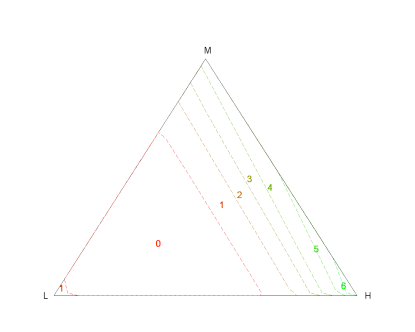
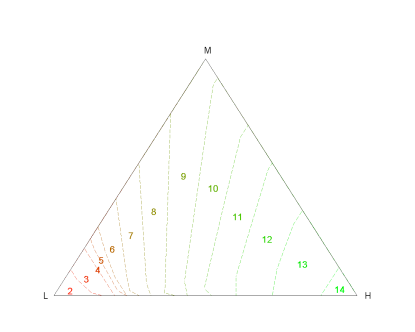
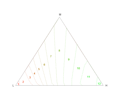
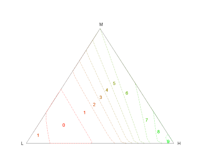
Figure 2. Optimal inventory levels for different time horizons for Section 4.1. We plot the regions of constancy for d(T,π)=argmaxaU(T,π,a)superscript𝑑𝑇𝜋subscriptargmax𝑎𝑈𝑇𝜋𝑎d^{*}(T,\vec{\pi})=\operatorname{argmax}_{a}U(T,\vec{\pi},a), which is the optimal inventory level to maintain given beliefs π𝜋\vec{\pi} (since ordering costs are zero), πD={π1+π2+π3=1}𝜋𝐷subscript𝜋1subscript𝜋2subscript𝜋31\vec{\pi}\in D=\{\pi_{1}+\pi_{2}+\pi_{3}=1\}. Top panels: K(a)=2a𝐾𝑎2𝑎K(a)=2a, bottom panels K(a)=4a𝐾𝑎4𝑎K(a)=4a; left panels: T=1𝑇1T=1, right panels: T=5𝑇5T=5.

Figure 2 illustrates these phenomena as we vary the relative stockout costs K(a)𝐾𝑎K(a), and the remaining horizon. We show four panels where horizontally the horizon changes and vertically the stock-out penalty K𝐾K changes. We observe that K𝐾K has a dramatic effect on optimal inventory level (note that in this example ordering costs are zero, so the optimal policy is only driven by K𝐾K and c𝑐c). Also note that the region where optimal policy is d(T,π)=1superscript𝑑𝑇𝜋1d^{*}(T,\vec{\pi})=1 is disjoint in the top two panels.

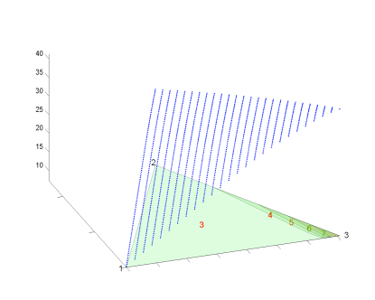
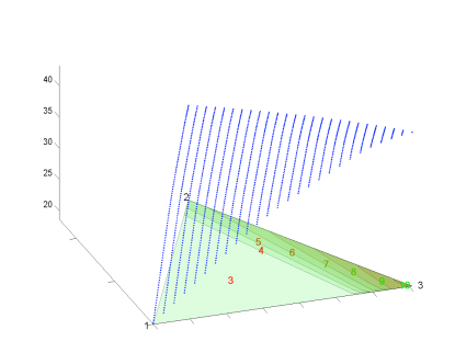
Figure 3 again follows [30] and shows the effect of different time dynamics of core process M𝑀M. In the first case, we assume that demands are expected to increase over time, so that the transition of M𝑀M follows the phases 1231231\to 2\to 3. In that case, it is possible that inventory will be increased even without any new events (i.e. τkσsubscript𝜏𝑘subscript𝜎\tau_{k}\neq\sigma_{\ell}). This happens because passage of time implies that the conditional probability Π(3)=(Mt=3|𝔽tW)superscriptΠ3subscript𝑀𝑡conditional3superscriptsubscript𝔽𝑡𝑊\vec{\Pi}^{(3)}=\mathbb{P}(M_{t}=3|\mathbb{F}_{t}^{W}) increases, and to counteract the corresponding increase in probability of a stock-out, new inventory might be ordered. In the second case, we assume that demand will be decreasing over time. In that case, the controller will order less compared to base case, since chances of overstocking will be increased.
Refer to caption Refer to caption
Figure 3. Optimal inventory levels for different core process dynamics in [30] (TS02) example of Section 4.1. The blue surfaces show U(T,π,3)𝑈𝑇𝜋3U(T,\vec{\pi},3) over the triangle πD={π1+π2+π3=1}𝜋𝐷subscript𝜋1subscript𝜋2subscript𝜋31\vec{\pi}\in D=\{\pi_{1}+\pi_{2}+\pi_{3}=1\}; underneath we show the optimal inventory levels d(T,π)superscript𝑑𝑇𝜋d^{*}(T,\vec{\pi}), see Figure 2. Left panel (case US in TS02): Q=(0.20.10.100.20.2000)𝑄0.20.10.100.20.2000Q=\left(\begin{smallmatrix}-0.2&0.1&0.1\\ 0&-0.2&0.2\\ 0&0&0\end{smallmatrix}\right), right panel (case DS in TS02): Q=(0000.20.200.10.10.2)𝑄0000.20.200.10.10.2Q=\left(\begin{smallmatrix}0&0&0\\ 0.2&-0.2&0\\ 0.1&0.1&-0.2\end{smallmatrix}\right). (Note that in TS02 time is discrete. To be able to make a comparison we choose our generators to make the average holding time in each state equal to those of TS02.)

4.2. Example with Censoring

In our second example we consider a model that treats censored observations. We assume that excess demand above available stock is unobserved, and that a corresponding opportunity cost is incurred in case of stock-out.

For parameters we choose

Q=(1111),λ=(21),ν=(0.50.40.10.10.30.6),formulae-sequence𝑄matrix1111formulae-sequence𝜆matrix21𝜈matrix0.50.40.10.10.30.6Q=\begin{pmatrix}-1&1\\ 1&-1\end{pmatrix},\qquad\vec{\lambda}=\begin{pmatrix}2\\ 1\end{pmatrix},\qquad\vec{\nu}=\begin{pmatrix}0.5&0.4&0.1\\ 0.1&0.3&0.6\end{pmatrix},

so that demands are of size at most R=3𝑅3R=3. Note that in regime 2, demands are less frequent but of larger size; also to distinguish between regimes it is crucial to observe the full demand size.

The horizon is T=3𝑇3T=3 and costs are selected as

c(a)=2a,K(a)=3.2a,h=1.25,ζ=1,formulae-sequence𝑐𝑎2𝑎formulae-sequence𝐾𝑎3.2𝑎formulae-sequence1.25𝜁1c(a)=2a,\qquad K(a)=3.2a,\qquad h=1.25,\qquad\zeta=1,

with P¯=R=3¯𝑃𝑅3\overline{P}=R=3. Again, we consider zero salvage value. These parameters have been specially chosen to emphasize the effect of censoring.

We find that the effect of censoring on the value function U𝑈U is on the order of 3-4% in this example, see Table 2 below. However, this obscures the fact that the optimal policies are dramatically different in the two cases. Figure 4 compares the two optimal policies given that current inventory is empty. In general, as might be expected, censored observations cause the manager to carry extra inventory in order to obtain maximum information. However, counter-intuitively, there are also values of t𝑡t and π𝜋\vec{\pi} where censoring can lead to lower inventory (compared to no-censoring). We have observed situations where censoring increases inventory costs by up to 15%, which highlights the need to properly model that feature (the particular example was included to showcase other features we observe below).
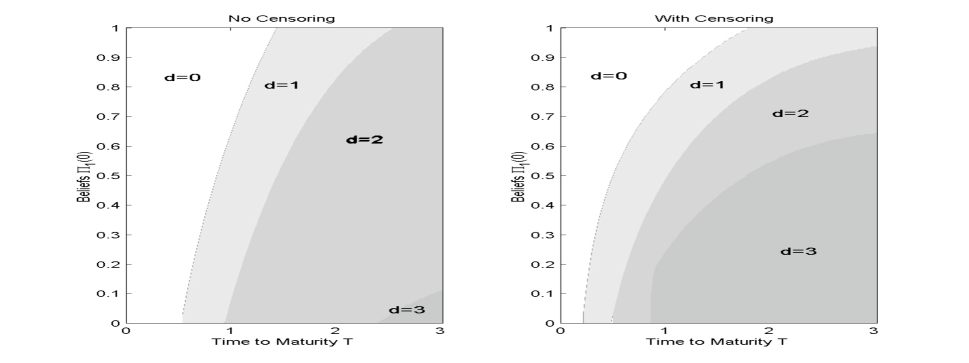
Refer to caption
Figure 4. Optimal order levels as a function of time and beliefs given current empty inventory, P(0)=0𝑃00P(0)=0. We plot dU(T,π,0)subscript𝑑𝑈𝑇𝜋0d_{\mathcal{M}U}(T,\vec{\pi},0) as a function of time to maturity T𝑇T on the x-axis and initial beliefs Π1(0)=(M0=1)subscriptΠ10subscript𝑀01\Pi_{1}(0)=\mathbb{P}(M_{0}=1) on the y-axis.

4.3. Optimal Strategy Implementation

In Figure 5, we present a sample path of the (Π,P)Π𝑃(\vec{\Pi},P)-process which shows the implementation of the optimal policy as defined in Figure 4. We consider the above setting with censored observations, T=3𝑇3T=3 initial Π1(0)=0.6subscriptΠ100.6\Pi_{1}(0)=0.6 (since Π2(t)1Π1(t)subscriptΠ2𝑡1subscriptΠ1𝑡\Pi_{2}(t)\equiv 1-\Pi_{1}(t) in this one-dimensional example, we focus on just the first component Π1(t)=(Mt=1)subscriptΠ1𝑡subscript𝑀𝑡1\Pi_{1}(t)=\mathbb{P}(M_{t}=1)) and initial zero inventory, P(0)=0𝑃00P(0)=0. In this example, it is optimal for the manager to place new orders only when inventory is completely exhausted. Thus, dU(T,π,a)subscript𝑑𝑈𝑇𝜋𝑎d_{\mathcal{M}U}(T,\vec{\pi},a) is non-trivial only for a=0𝑎0a=0; otherwise we have dU(T,π,a)=asubscript𝑑𝑈𝑇𝜋𝑎𝑎d_{\mathcal{M}U}(T,\vec{\pi},a)=a and the manager should just wait.

Since dU(3,Π(0),0)=3subscript𝑑𝑈3Π003d_{\mathcal{M}U}(3,\vec{\Pi}(0),0)=3, it is optimal for the manager to immediately put an order for three units, as indicated by an arrow on the y-axis in Figure 5. Then the manager waits for demand orders, in the meantime paying storage costs on the three units on inventory. At time σ1subscript𝜎1\sigma_{1}, the first demand order (in this case of size two arrives). This results in the update of the beliefs according to Proposition (2.1) as

Π1(σ1)=λ1ν1(2)Π1(σ1)i=12λiνi(2)Πi(σ1)=20.4Π1(σ1)20.4Π1(σ1)+10.3(1Π1(σ1)).subscriptΠ1subscript𝜎1subscript𝜆1subscript𝜈12subscriptΠ1limit-fromsubscript𝜎1superscriptsubscript𝑖12subscript𝜆𝑖subscript𝜈𝑖2subscriptΠ𝑖limit-fromsubscript𝜎120.4subscriptΠ1limit-fromsubscript𝜎120.4subscriptΠ1limit-fromsubscript𝜎110.31subscriptΠ1limit-fromsubscript𝜎1\Pi_{1}(\sigma_{1})=\frac{\lambda_{1}\cdot\nu_{1}(2)\cdot\Pi_{1}(\sigma_{1}-)}{\sum_{i=1}^{2}\lambda_{i}\cdot\nu_{i}(2)\cdot\Pi_{i}(\sigma_{1}-)}=\frac{2\cdot 0.4\cdot\Pi_{1}(\sigma_{1}-)}{2\cdot 0.4\cdot\Pi_{1}(\sigma_{1}-)+1\cdot 0.3\cdot(1-\Pi_{1}(\sigma_{1}-))}.

This demand is fully observed and filled; since dU(3σ1,Πσ1,1)=1subscript𝑑𝑈3subscript𝜎1subscriptΠsubscript𝜎111d_{\mathcal{M}U}(3-\sigma_{1},\vec{\Pi}_{\sigma_{1}},1)=1, no new orders are placed at that time. Then at time σ2subscript𝜎2\sigma_{2} we assume that a censored demand (i.e. a demand of size more than 1 arrives). This time the update in the beliefs is

Π1(σ2)=λ1[ν1(2)+ν1(3)]Π1(σ2)i=12λi[νi(2)+νi(3)]Πi(σ2)=20.5Π1(σ2)20.5Π1(σ2)+10.9(1Π1(σ2)).subscriptΠ1subscript𝜎2subscript𝜆1delimited-[]subscript𝜈12subscript𝜈13subscriptΠ1limit-fromsubscript𝜎2superscriptsubscript𝑖12subscript𝜆𝑖delimited-[]subscript𝜈𝑖2subscript𝜈𝑖3subscriptΠ𝑖limit-fromsubscript𝜎220.5subscriptΠ1limit-fromsubscript𝜎220.5subscriptΠ1limit-fromsubscript𝜎210.91subscriptΠ1limit-fromsubscript𝜎2\Pi_{1}(\sigma_{2})=\frac{\lambda_{1}\cdot[\nu_{1}(2)+\nu_{1}(3)]\cdot\Pi_{1}(\sigma_{2}-)}{\sum_{i=1}^{2}\lambda_{i}\cdot[\nu_{i}(2)+\nu_{i}(3)]\cdot\Pi_{i}(\sigma_{2}-)}=\frac{2\cdot 0.5\cdot\Pi_{1}(\sigma_{2}-)}{2\cdot 0.5\cdot\Pi_{1}(\sigma_{2}-)+1\cdot 0.9\cdot(1-\Pi_{1}(\sigma_{2}-))}.

We see that the censored observation gives very little new information to the manager and Π1(σ2)subscriptΠ1subscript𝜎2\Pi_{1}(\sigma_{2}) is close to Π1(σ2)subscriptΠ1limit-fromsubscript𝜎2\Pi_{1}(\sigma_{2}-). The inventory is now instantaneously brought down to zero, as the one remaining unit is shipped out (and the rest is assigned an expected lost opportunity cost). Because dU(Tσ2,Π(σ2),0)=1subscript𝑑𝑈𝑇subscript𝜎2Πsubscript𝜎201d_{\mathcal{M}U}(T-\sigma_{2},\vec{\Pi}(\sigma_{2}),0)=1, the manager immediately orders one new unit of inventory, τ1=σ2subscript𝜏1subscript𝜎2\tau_{1}=\sigma_{2}. Thus, overall we end up with P(σ2)=1𝑃subscript𝜎21P(\sigma_{2})=1. At time σ3subscript𝜎3\sigma_{3}, a single unit demand (uncensored) is observed; this strongly suggests that Mσ3=1subscript𝑀subscript𝜎31M_{\sigma_{3}}=1 (due to short time between orders and a small order amount), and Π1(σ3)subscriptΠ1subscript𝜎3\Pi_{1}(\sigma_{3}) is indeed large. Given that little time remains till maturity, it is now optimal to place no more new orders, dU(Tσ3,Π(σ3),0)=0subscript𝑑𝑈𝑇subscript𝜎3Πsubscript𝜎300d_{\mathcal{M}U}(T-\sigma_{3},\vec{\Pi}(\sigma_{3}),0)=0. However, as time elapses, (Mt=2)subscript𝑀𝑡2\mathbb{P}(M_{t}=2) grows and the manager begins to worry about incurring excessive stock-out costs if a large order arrives. Accordingly, at time τ22.19similar-tosubscript𝜏22.19\tau_{2}\sim 2.19 (and without new incoming orders) the manager places an order for a new unit of inventory as (Π,P)Π𝑃(\vec{\Pi},P) again enters the region where dU=1subscript𝑑𝑈1d_{\mathcal{M}U}=1 (see lowermost panel of Figure 5). As it turns out in this sample, no new orders are in fact forthcoming until T𝑇T and the manager will lose the latter inventory as there are no salvage opportunities.
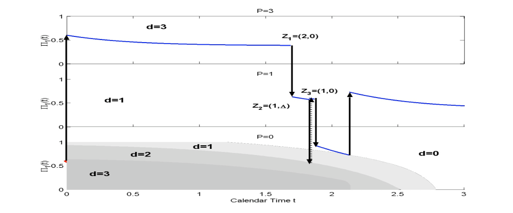
Refer to caption
Figure 5. Implementation of optimal strategy on a sample path. We plot the beliefs Π1(t)=(Mt=1)subscriptΠ1𝑡subscript𝑀𝑡1\Pi_{1}(t)=\mathbb{P}(M_{t}=1) as a function of calendar time t𝑡t, over the different panels corresponding to P(t)𝑃𝑡P(t). Incoming demand orders and placed supply orders are indicated with circles and diamonds respectively. Here T=3𝑇3T=3 and Π(0)=[0.6,0.4]Π00.60.4\vec{\Pi}(0)=[0.6,0.4]. The arrival times are σ1=1.7,σ2=1.83,σ3=1.87formulae-sequencesubscript𝜎11.7formulae-sequencesubscript𝜎21.83subscript𝜎31.87\sigma_{1}=1.7,\sigma_{2}=1.83,\sigma_{3}=1.87 and the corresponding marks are Z1=(2,0),Z2=(1,Δ),Z3=(1,0)formulae-sequencesubscript𝑍120formulae-sequencesubscript𝑍21Δsubscript𝑍310Z_{1}=(2,0),Z_{2}=(1,\Delta),Z_{3}=(1,0), see Section 2.4.

4.4. Effect of Other Parameters

We now compare the effects of other model parameters and ingredients on the value function and optimal strategy. To give a concise summary of our findings, Table 2 shows the initial value function and initial optimal policy for one fixed choice of beliefs Π(0)Π0\vec{\Pi}(0) and time-horizon T𝑇T.

In particular, we compare the effect of censoring, as well as changes in various costs on the value function and a representative optimal policy choice. We also study the effect of salvage opportunities and possibility of selling inventory. Salvaging at x% means that one adds the initial condition U(0,π,a)=xha𝑈0𝜋𝑎𝑥𝑎U(0,\vec{\pi},a)=-x\cdot h\cdot a to (2.5), so that at the terminal date the manager can recover some of the unit costs associated with unsold inventory. Selling inventory means that at any point in time the manager can sell back unneeded inventory, so that ξk{P(τk),,P¯P(τk)}subscript𝜉𝑘𝑃subscript𝜏𝑘¯𝑃𝑃subscript𝜏𝑘\xi_{k}\in\{-P(\tau_{k}),\ldots,\overline{P}-P(\tau_{k})\} and the minimization in (3.13) is over all b[0,P¯]𝑏0¯𝑃b\in[0,\overline{P}].

As expected, storage costs increase average costs and cause the manager to carry less inventory; conversely stock-out costs cause the manager to carry more inventory (and also increase the value function). Fixed order costs are also crucial and increase supply order sizes, as each supply order is very costly to place. We find that in this example, the possibility of salvaging inventory and opportunity to sell inventory have little impact on the value function, which appears to be primarily driven by potential stock-out penalties.

Model Value Function U(T,π,0)𝑈𝑇𝜋0U(T,\vec{\pi},0) Optimal Policy dU(T,π,0)subscript𝑑𝑈𝑇𝜋0d_{\mathcal{M}U}(T,\vec{\pi},0)
Base case w/out censoring 25.21 2
Base case w/censoring 25.97 3
Reduced stockout costs K(a)=2a𝐾𝑎2𝑎K(a)=2a 16.37 0
Zero storage costs c=0𝑐0c=0 16.71 3
No fixed ordering costs 22.92 1
Terminal salvage value of 50% 24.75 2
Can buy/sell at cost, ζ=1𝜁1\zeta=1 24.30 2
Table 2. Results for the comparative statics in Section 4.4. Here T=3𝑇3T=3 and Π(0)=π=(0.5,0.5)Π0𝜋0.50.5\vec{\Pi}(0)=\vec{\pi}=(0.5,0.5), so that (M0=1)=(M0=2)=12subscript𝑀01subscript𝑀0212\mathbb{P}(M_{0}=1)=\mathbb{P}(M_{0}=2)=\frac{1}{2}.

5. Conclusion

In this paper we have presented a probabilistic model that can address the setting of partially observed non-stationary demand in inventory management. Applying the DP intuition, we have derived and gave a direct proof the dynamic programming equation for the value function and the ensuing characterization of an optimal policy. We have also derived an alternative characterization that can be easily implemented on a computer. This gives a method to compute the full value function/optimal policy to any degree of accuracy. As such, our model contrasts with other approaches that only present heuristic policy choices.

Our model can also incorporate demand censoring. Our numerical investigations suggest that censored demands may have a significant influence on the optimal value to extract and even a more dramatic impact on the manager’s optimal policies. This highlights the need to properly model demand censoring in applications. It would be of interest to further study this aspect of the model and to compare it with real-life experiences of inventory managers.

Appendix A Proof of Proposition A.2

A.1. A Preliminary Result

Lemma A.1.

For iE𝑖𝐸i\in E, let us define

(A.1) Liπ,a,ξ(t,r:(tk,zk),kr)𝔼π,a,ξ[1{Mt=i}eI(t)k=1r(tk,zk)],\displaystyle L_{i}^{\vec{\pi},a,\xi}(t,r:(t_{k},\vec{z}_{k}),k\leq r)\triangleq\mathbb{E}^{\vec{\pi},a,\xi}\left[1_{\{M_{t}=i\}}\cdot\mathrm{e}^{-I(t)}\cdot\prod_{k=1}^{r}\ell(t_{k},\vec{z}_{k})\right],

where

(A.2) (t,z)jE1{Mt=j}λjgj(z;Pt).𝑡𝑧subscript𝑗𝐸subscript1subscript𝑀𝑡𝑗subscript𝜆𝑗subscript𝑔𝑗𝑧subscript𝑃limit-from𝑡\displaystyle\ell(t,\vec{z})\triangleq\sum_{j\in E}1_{\{M_{t}=j\}}\lambda_{j}\cdot g_{j}(\vec{z};P_{t-}).

Moreover let Lπ,a,ξ(t,r:(tk,zk),kr)=jELjπ,a,ξ(t,r:(tk,zk),kr)L^{\vec{\pi},a,\xi}(t,r:(t_{k},\vec{z}_{k}),k\leq r)=\sum_{j\in E}L_{j}^{\vec{\pi},a,\xi}(t,r:(t_{k},\vec{z}_{k}),k\leq r). Then we have

(A.3) Πi(t)subscriptΠ𝑖𝑡\displaystyle\Pi_{i}(t) =Liπ,a,ξ(t,Nt:(σk,Zk),kNt)Lπ(t,Nt:(σk,Zk),kNt)[Liπ,a,ξ(t,r:(tk,zk),kr)Lπ,a,ξ(t,r:(tk,zk),kr)]|r=Nt;(tk=σk,zk=Zk)kr\displaystyle=\frac{L_{i}^{\vec{\pi},a,\xi}(t,N_{t}:(\sigma_{k},Z_{k}),k\leq N_{t})}{L^{\vec{\pi}}(t,N_{t}:(\sigma_{k},Z_{k}),k\leq N_{t})}\equiv\left[\frac{L_{i}^{\vec{\pi},a,\xi}(t,r:(t_{k},\vec{z}_{k}),k\leq r)}{L^{\vec{\pi},a,\xi}(t,r:(t_{k},\vec{z}_{k}),k\leq r)}\right]\Bigg{|}_{r=N_{t}\,;\,(t_{k}=\sigma_{k},\vec{z}_{k}=Z_{k})_{k\leq r}}

πsuperscript𝜋\mathbb{P}^{\vec{\pi}}-a.s., for all t0𝑡0t\geq 0, and for iE𝑖𝐸i\in E.

Proof.

Let ΞΞ\Xi be a set of the form

Ξ={Nt1=r1,,Ntk=rk;(Z1,,Zrk)B}Ξformulae-sequencesubscript𝑁subscript𝑡1subscript𝑟1formulae-sequencesubscript𝑁subscript𝑡𝑘subscript𝑟𝑘subscript𝑍1subscript𝑍subscript𝑟𝑘𝐵\displaystyle{\Xi}=\{N_{t_{1}}=r_{1},\ldots,N_{t_{k}}=r_{k};(Z_{1},\ldots,Z_{r_{k}})\in B\}

where 0=t0t1tk=t0subscript𝑡0subscript𝑡1subscript𝑡𝑘𝑡0=t_{0}\leq t_{1}\leq\ldots\leq t_{k}=t with 0r1rk0subscript𝑟1subscript𝑟𝑘0\leq r_{1}\leq\ldots\leq r_{k} for k𝑘k\in\mathbb{N}, and B𝐵B is a Borel set in (rk)superscriptsubscript𝑟𝑘\mathcal{B}(\mathbb{R}^{r_{k}}). Since tjsubscript𝑡𝑗t_{j} and rjsubscript𝑟𝑗r_{j}’s are arbitrary, to prove (A.3) by the Monotone Class Theorem it is then sufficient to establish

𝔼π,a,ξ[1Ξπ{Mt=i|tW}]=𝔼π,a,ξ[1ΞLiπ,a,ξ(t,Nt:(σk,Zk),kNt)Lπ,a,ξ(t,Nt:(σk,Zk),kNt)].\displaystyle\mathbb{E}^{\vec{\pi},a,\xi}\left[1_{\Xi}\cdot\mathbb{P}^{\vec{\pi}}\{M_{t}=i|\mathcal{F}^{W}_{t}\}\right]=\mathbb{E}^{\vec{\pi},a,\xi}\left[1_{\Xi}\cdot\frac{L_{i}^{\vec{\pi},a,\xi}(t,N_{t}:(\sigma_{k},Z_{k}),k\leq N_{t})}{L^{\vec{\pi},a,\xi}(t,N_{t}:(\sigma_{k},Z_{k}),k\leq N_{t})}\right].

Conditioning on the path of M𝑀M, the left-hand side (LHS) above equals

LHS=𝔼π,a,ξ[1{Mt=i}π{Nt1=r1,,Ntk=rk;(Z1,,Zrk)B|Ms,st}]=𝔼π,a,ξ[1{Mt=i}B×Υ(t1,,tk)π{σ1ds1,,σrkdsrk;Z1=z1,,Zrk=zrk|Ms,st}]𝐿𝐻𝑆superscript𝔼𝜋𝑎𝜉delimited-[]subscript1subscript𝑀𝑡𝑖superscript𝜋conditional-setformulae-sequencesubscript𝑁subscript𝑡1subscript𝑟1formulae-sequencesubscript𝑁subscript𝑡𝑘subscript𝑟𝑘subscript𝑍1subscript𝑍subscript𝑟𝑘𝐵subscript𝑀𝑠𝑠𝑡superscript𝔼𝜋𝑎𝜉delimited-[]subscript1subscript𝑀𝑡𝑖subscript𝐵Υsubscript𝑡1subscript𝑡𝑘superscript𝜋conditional-setformulae-sequencesubscript𝜎1𝑑subscript𝑠1formulae-sequencesubscript𝜎subscript𝑟𝑘𝑑subscript𝑠subscript𝑟𝑘formulae-sequencesubscript𝑍1subscript𝑧1subscript𝑍subscript𝑟𝑘subscript𝑧subscript𝑟𝑘subscript𝑀𝑠𝑠𝑡LHS=\mathbb{E}^{\vec{\pi},a,\xi}\left[1_{\{M_{t}=i\}}\mathbb{P}^{\vec{\pi}}\left\{N_{t_{1}}=r_{1},\ldots,N_{t_{k}}=r_{k};(Z_{1},\ldots,Z_{r_{k}})\in B\,\Big{|}M_{s},\,s\leq t\ \right\}\right]=\\ \mathbb{E}^{\vec{\pi},a,\xi}\left[1_{\{M_{t}=i\}}\int_{B\times\Upsilon(t_{1},\dotsc,t_{k})}\mathbb{P}^{\vec{\pi}}\left\{\sigma_{1}\in ds_{1},\ldots,\sigma_{r_{k}}\in ds_{r_{k}};Z_{1}=\vec{z}_{1},\ldots,Z_{r_{k}}=\vec{z}_{r_{k}}\,\Big{|}M_{s},\,s\leq t\ \right\}\right]

where

Υ(t1,,tk)={s1,,srk+rk:s1srktandsrjtj<srj+1forj=1,k}.Υsubscript𝑡1subscript𝑡𝑘conditional-setsubscript𝑠1subscript𝑠subscript𝑟𝑘superscriptsubscriptsubscript𝑟𝑘formulae-sequencesubscript𝑠1subscript𝑠subscript𝑟𝑘𝑡andsubscript𝑠subscript𝑟𝑗subscript𝑡𝑗subscript𝑠subscript𝑟𝑗1for𝑗1𝑘\displaystyle\Upsilon(t_{1},\dotsc,t_{k})=\left\{s_{1},\ldots,s_{r_{k}}\in\mathbb{R}_{+}^{r_{k}}:\;s_{1}\leq\ldots\leq s_{r_{k}}\leq t\;\;\text{and}\;\;s_{r_{j}}\leq t_{j}<s_{r_{j}+1}\;\text{for}\;j=1,\ldots k\right\}.

Then, using (2.10) and Fubini’s theorem we obtain

LHS𝐿𝐻𝑆\displaystyle LHS =𝔼π,a,ξ[1{Mt=i}B×Υ(t1,,tk)eI(t)=1rkjE1{Ms=j}λjgj(z;Ps)ds]absentsuperscript𝔼𝜋𝑎𝜉delimited-[]subscript1subscript𝑀𝑡𝑖subscript𝐵Υsubscript𝑡1subscript𝑡𝑘superscripte𝐼𝑡superscriptsubscriptproduct1subscript𝑟𝑘subscript𝑗𝐸subscript1subscript𝑀subscript𝑠𝑗subscript𝜆𝑗subscript𝑔𝑗subscript𝑧subscript𝑃subscript𝑠𝑑subscript𝑠\displaystyle=\mathbb{E}^{\vec{\pi},a,\xi}\left[1_{\{M_{t}=i\}}\int_{B\times\Upsilon(t_{1},\dotsc,t_{k})}\mathrm{e}^{-I(t)}\prod_{\ell=1}^{r_{k}}\sum_{j\in E}1_{\{M_{s_{\ell}}=j\}}\lambda_{j}g_{j}(\vec{z}_{\ell};P_{s_{\ell}})\,ds_{\ell}\,\right]
=B×Υ(t1,,tk)𝔼π,a,ξ[1{Mt=i}eI(t)=1rkjE1{Ms=j}λjgj(z;Ps)]=1rkdsabsentsubscript𝐵Υsubscript𝑡1subscript𝑡𝑘superscript𝔼𝜋𝑎𝜉delimited-[]subscript1subscript𝑀𝑡𝑖superscripte𝐼𝑡superscriptsubscriptproduct1subscript𝑟𝑘subscript𝑗𝐸subscript1subscript𝑀subscript𝑠𝑗subscript𝜆𝑗subscript𝑔𝑗subscript𝑧subscript𝑃subscript𝑠superscriptsubscriptproduct1subscript𝑟𝑘𝑑subscript𝑠\displaystyle=\int_{B\times\Upsilon(t_{1},\dotsc,t_{k})}\mathbb{E}^{\vec{\pi},a,\xi}\left[1_{\{M_{t}=i\}}\mathrm{e}^{-I(t)}\prod_{\ell=1}^{r_{k}}\sum_{j\in E}1_{\{M_{s_{\ell}}=j\}}\lambda_{j}g_{j}(\vec{z}_{\ell};P_{s_{\ell}})\right]\prod_{\ell=1}^{r_{k}}ds_{\ell}
=B×Υ(t1,,tk)Liπ,a,ξ(t,rk:(sj,zj),jrk)=1rkds\displaystyle=\int_{B\times\Upsilon(t_{1},\dotsc,t_{k})}L_{i}^{\vec{\pi},a,\xi}(t,r_{k}:(s_{j},\vec{z}_{j}),j\leq r_{k})\prod_{\ell=1}^{r_{k}}ds_{\ell}
=B×Υ(t1,,tk)Liπ,a,ξ(t,rk:(sj,zj),jrk)Lπ,a,ξ(t,rk:(σj,Yj),jrk)Lπ,a,ξ(t,rk:(sj,zj),jrk)=1rkds\displaystyle=\int_{B\times\Upsilon(t_{1},\dotsc,t_{k})}\frac{L_{i}^{\vec{\pi},a,\xi}(t,r_{k}:(s_{j},\vec{z}_{j}),j\leq r_{k})}{L^{\vec{\pi},a,\xi}(t,r_{k}:(\sigma_{j},Y_{j}),j\leq r_{k})}\cdot L^{\vec{\pi},a,\xi}(t,r_{k}:(s_{j},\vec{z}_{j}),j\leq r_{k})\prod_{\ell=1}^{r_{k}}ds_{\ell}
=B×Υ(t1,,tk)Liπ,a,ξ()Lπ,a,ξ()𝔼π[iE1{Mt=i}eI(t)=1rkjE1{Ms=j}λjgj(zl;Ps)]=1rkds.absentsubscript𝐵Υsubscript𝑡1subscript𝑡𝑘superscriptsubscript𝐿𝑖𝜋𝑎𝜉superscript𝐿𝜋𝑎𝜉superscript𝔼𝜋delimited-[]subscript𝑖𝐸subscript1subscript𝑀𝑡𝑖superscripte𝐼𝑡superscriptsubscriptproduct1subscript𝑟𝑘subscript𝑗𝐸subscript1subscript𝑀subscript𝑠𝑗subscript𝜆𝑗subscript𝑔𝑗subscript𝑧𝑙subscript𝑃subscript𝑠superscriptsubscriptproduct1subscript𝑟𝑘𝑑subscript𝑠\displaystyle=\int_{B\times\Upsilon(t_{1},\dotsc,t_{k})}\frac{L_{i}^{\vec{\pi},a,\xi}(\ldots)}{L^{\vec{\pi},a,\xi}(\ldots)}\cdot\mathbb{E}^{\vec{\pi}}\left[\sum_{i\in E}1_{\{M_{t}=i\}}\mathrm{e}^{-I(t)}\prod_{\ell=1}^{r_{k}}\sum_{j\in E}1_{\{M_{s_{\ell}}=j\}}\lambda_{j}g_{j}(\vec{z}_{l};P_{s_{\ell}})\right]\prod_{\ell=1}^{r_{k}}ds_{\ell}.

By another application of Fubini’s theorem, we obtain LHS=𝐿𝐻𝑆absentLHS=

𝔼π,a,ξ[iE1{Mt=i}B×Υ(t1,,tk)Liπ,a,ξ(t,rk:(sj,zj),jrk)Lπ,a,ξ(t,rk:(σj,zj),jrk)eI(t)=1rkjE1{Ms=i}λjgj(z;Ps)=1rkds]\displaystyle\mathbb{E}^{\vec{\pi},a,\xi}\left[\sum_{i\in E}1_{\{M_{t}=i\}}\int_{B\times\Upsilon(t_{1},\dotsc,t_{k})}\frac{L_{i}^{\vec{\pi},a,\xi}(t,r_{k}:(s_{j},\vec{z}_{j}),j\leq r_{k})}{L^{\vec{\pi},a,\xi}(t,r_{k}:(\sigma_{j},\vec{z}_{j}),j\leq r_{k})}\cdot\mathrm{e}^{-I(t)}\prod_{\ell=1}^{r_{k}}\sum_{j\in E}1_{\{M_{s_{\ell}}=i\}}\lambda_{j}g_{j}(\vec{z}_{\ell};P_{s_{\ell}})\cdot\prod_{\ell=1}^{r_{k}}ds_{\ell}\right]
=𝔼π,a,ξ[iE1{Mt=i}𝔼π,a,ξ[1{Nt1=r1,,Ntk=rk;(Z1,,Zrk)B}Liπ,a,ξ(t,Nt:(σj,Zj),jNt)Lπ,a,ξ(t,Nt:(σj,Zj),jNt)|Ms;st]]\displaystyle=\mathbb{E}^{\vec{\pi},a,\xi}\left[\sum_{i\in E}1_{\{M_{t}=i\}}\mathbb{E}^{\vec{\pi},a,\xi}\left[1_{\{N_{t_{1}}=r_{1},\ldots,N_{t_{k}}=r_{k};(Z_{1},\ldots,Z_{r_{k}})\in B\}}\cdot\frac{L_{i}^{\vec{\pi},a,\xi}(t,N_{t}:(\sigma_{j},Z_{j}),j\leq N_{t})}{L^{\vec{\pi},a,\xi}(t,N_{t}:(\sigma_{j},Z_{j}),j\leq N_{t})}\;\Bigg{|}M_{s};\,s\leq t\right]\right]
=𝔼π,a,ξ[𝔼π,a,ξ[1{Nt1=r1,,Ntk=rk;(Z1,,Zrk)B}Liπ,a,ξ(t,Nt:(σj,Zj),jNt)Lπ,a,ξ(t,Nt:(σj,Zj),jNt)|Ms;st]]\displaystyle=\mathbb{E}^{\vec{\pi},a,\xi}\left[\mathbb{E}^{\vec{\pi},a,\xi}\left[1_{\{N_{t_{1}}=r_{1},\ldots,N_{t_{k}}=r_{k};(Z_{1},\ldots,Z_{r_{k}})\in B\}}\cdot\frac{L_{i}^{\vec{\pi},a,\xi}(t,N_{t}:(\sigma_{j},Z_{j}),j\leq N_{t})}{L^{\vec{\pi},a,\xi}(t,N_{t}:(\sigma_{j},Z_{j}),j\leq N_{t})}\;\Bigg{|}M_{s};\,s\leq t\right]\right]
=𝔼π,a,ξ[1ΞLiπ,a,ξ(t,Nt:(σj,Zj),jNt)Lπ,a,ξ(t,Nt:(σj,Zj),jNt)].\displaystyle=\mathbb{E}^{\vec{\pi},a,\xi}\left[1_{\Xi}\cdot\frac{L_{i}^{\vec{\pi},a,\xi}(t,N_{t}:(\sigma_{j},Z_{j}),j\leq N_{t})}{L^{\vec{\pi},a,\xi}(t,N_{t}:(\sigma_{j},Z_{j}),j\leq N_{t})}\right].

A.2. Proof of Proposition 2.1

Let 𝔼ja,ξ[]subscriptsuperscript𝔼𝑎𝜉𝑗delimited-[]\mathbb{E}^{a,\xi}_{j}[\cdot] denote the expectation operator 𝔼π,a,ξ[|M0=j]\mathbb{E}^{\vec{\pi},a,\xi}[\cdot\,|M_{0}=j], and let trtt+usubscript𝑡𝑟𝑡𝑡𝑢t_{r}\leq t\leq t+u, then

(A.4) Liπ,a,ξ(t+u,r:(tk,zk),kr)=jEπj𝔼ja,ξ[1{Mt+u=i}eI(t+u)k=1r(tk,zk)]=jEπj𝔼ja,ξ[𝔼ja,ξ[1{Mt+u=i}eI(t+u)k=1r(tk,zk)|Ms,st]]=jEπj𝔼ja,ξ[eI(t)(k=1r(tk,zk))𝔼ja,ξ[1{Mt+u=i}e(I(t+u)I(t))|Mt]],L_{i}^{\vec{\pi},a,\xi}(t+u,r:(t_{k},\vec{z}_{k}),k\leq r)=\sum_{j\in E}\pi_{j}\cdot\mathbb{E}^{a,\xi}_{j}\left[1_{\{M_{t+u}=i\}}\cdot\mathrm{e}^{-I(t+u)}\cdot\prod_{k=1}^{r}\ell(t_{k},\vec{z}_{k})\right]\\ \begin{aligned} =&\sum_{j\in E}\pi_{j}\cdot\mathbb{E}^{a,\xi}_{j}\left[\mathbb{E}^{a,\xi}_{j}\Biggl{[}1_{\{M_{t+u}=i\}}\cdot\mathrm{e}^{-I(t+u)}\cdot\prod_{k=1}^{r}\ell(t_{k},\vec{z}_{k})\,\Bigg{|}M_{s},s\leq t\Biggr{]}\right]\\ =&\sum_{j\in E}\pi_{j}\cdot\mathbb{E}^{a,\xi}_{j}\left[\mathrm{e}^{-I(t)}\left(\prod_{k=1}^{r}\ell(t_{k},\vec{z}_{k})\right)\mathbb{E}^{a,\xi}_{j}\left[1_{\{M_{t+u}=i\}}\cdot\mathrm{e}^{-(I(t+u)-I(t))}\Bigg{|}M_{t}\right]\right],\end{aligned}

where the third equality followed from the properties of the conditional expectation and the Markov property of M𝑀M. The last expression in (A.4) can be written as

=jEπj𝔼ja,ξ[eI(t)(k=1r(tk,zk))lE1{Mt=l}𝔼la,ξ[1{Mu=i}eI(u)]]=lE𝔼la,ξ[1{Mu=i}eI(u)]𝔼π[1{Mt=l}eI(t)k=1r(tk,zk)]=lE𝔼la,ξ[1{Mu=i}eI(u)]Llπ(t,r:(tk,zk),kr).\begin{aligned} =&\sum_{j\in E}\pi_{j}\cdot\mathbb{E}^{a,\xi}_{j}\left[\mathrm{e}^{-I(t)}\left(\prod_{k=1}^{r}\ell(t_{k},\vec{z}_{k})\right)\cdot\sum_{l\in E}1_{\{M_{t}=l\}}\cdot\mathbb{E}^{a,\xi}_{l}\left[1_{\{M_{u}=i\}}\cdot\mathrm{e}^{-I(u)}\right]\right]\\ =&\sum_{l\in E}\mathbb{E}^{a,\xi}_{l}\left[1_{\{M_{u}=i\}}\cdot\mathrm{e}^{-I(u)}\right]\cdot\mathbb{E}^{\vec{\pi}}\left[1_{\{M_{t}=l\}}\cdot\mathrm{e}^{-I(t)}\prod_{k=1}^{r}\ell(t_{k},\vec{z}_{k})\right]\\ =&\sum_{l\in E}\mathbb{E}^{a,\xi}_{l}\left[1_{\{M_{u}=i\}}\cdot\mathrm{e}^{-I(u)}\right]\cdot L_{l}^{\vec{\pi}}(t,r:(t_{k},\vec{z}_{k}),k\leq r).\end{aligned}

Then the explicit form of ΠΠ\vec{\Pi} in (A.3) implies that for σmtt+u<σm+1subscript𝜎𝑚𝑡𝑡𝑢subscript𝜎𝑚1\sigma_{m}\leq t\leq t+u<\sigma_{m+1}, we have

(A.5) Πi(t+u)=lELlπ(t,r:(σk,zk),kr)𝔼la,ξ[1{Mu=i}eI(u)]jElELlπ(t,r:(σk,zk),kr)𝔼la,ξ[1{Mu=j}eI(u)]=lEΠl(t)𝔼la,ξ[1{Mu=i}eI(u)]jElEΠl(t)𝔼la,ξ[1{Mu=j}eI(u)]=𝔼Πt[1{Mu=i}eI(u)]jE𝔼Πt[1{Mu=j}eI(u)]=𝔼Πt[1{Mu=i}eI(u)]𝔼Πt[eI(u)]=π{σ1>u,Mu=i}π{σ1>u}|π=Πt.\displaystyle\begin{aligned} \Pi_{i}(t+u)&=\frac{\sum_{l\in E}L_{l}^{\vec{\pi}}(t,r:(\sigma_{k},\vec{z}_{k}),k\leq r)\cdot\mathbb{E}^{a,\xi}_{l}\left[1_{\{M_{u}=i\}}\cdot\mathrm{e}^{-I(u)}\right]}{\sum_{j\in E}\sum_{l\in E}L_{l}^{\vec{\pi}}(t,r:(\sigma_{k},\vec{z}_{k}),k\leq r)\cdot\mathbb{E}^{a,\xi}_{l}\left[1_{\{M_{u}=j\}}\cdot\mathrm{e}^{-I(u)}\right]}\\ &=\frac{\sum_{l\in E}\Pi_{l}(t)\cdot\mathbb{E}^{a,\xi}_{l}\left[1_{\{M_{u}=i\}}\cdot\mathrm{e}^{-I(u)}\right]}{\sum_{j\in E}\sum_{l\in E}\Pi_{l}(t)\cdot\mathbb{E}^{a,\xi}_{l}\left[1_{\{M_{u}=j\}}\cdot\mathrm{e}^{-I(u)}\right]}=\frac{\mathbb{E}^{\vec{\Pi}_{t}}\left[1_{\{M_{u}=i\}}\cdot\mathrm{e}^{-I(u)}\right]}{\sum_{j\in E}\mathbb{E}^{\vec{\Pi}_{t}}\left[1_{\{M_{u}=j\}}\cdot\mathrm{e}^{-I(u)}\right]}\\ &=\frac{\mathbb{E}^{\vec{\Pi}_{t}}\left[1_{\{M_{u}=i\}}\cdot\mathrm{e}^{-I(u)}\right]}{\mathbb{E}^{\vec{\Pi}_{t}}\left[\mathrm{e}^{-I(u)}\right]}=\frac{\mathbb{P}^{\vec{\pi}}\{\sigma_{1}>u,M_{u}=i\}}{\mathbb{P}^{\vec{\pi}}\{\sigma_{1}>u\}}\Bigg{|}_{\vec{\pi}=\vec{\Pi}_{t}}.\end{aligned}

On the other hand, the expression in (A.1) implies

(A.6) Liπ,a,ξ(σr+1,r+1:(σk,Zk),kr+1)=𝔼π,a,ξ[1{Mt=i}eI(t)k=1r+1(tk,zk)]|t=σr+1;(tk=σk,yk=Zk)kr+1=λigi(Zr+1;Pσr+1)𝔼π,a,ξ[1{Mt=i}eI(t)k=1r(tk,zk)]|t=σr+1;(tk=σk,zk=Zk)kr.L_{i}^{\vec{\pi},a,\xi}(\sigma_{r+1},r+1:(\sigma_{k},Z_{k}),k\leq r+1)=\mathbb{E}^{\vec{\pi},a,\xi}\left[1_{\{M_{t}=i\}}\cdot\mathrm{e}^{-I(t)}\cdot\prod_{k=1}^{r+1}\ell(t_{k},\vec{z}_{k})\right]\Bigg{|}_{t=\sigma_{r+1}\,;\,(t_{k}=\sigma_{k},y_{k}=Z_{k})_{k\leq r+1}}\\ \begin{aligned} =\lambda_{i}g_{i}(Z_{r+1};P_{\sigma_{r+1}-})\cdot\mathbb{E}^{\vec{\pi},a,\xi}\left[1_{\{M_{t}=i\}}\cdot\mathrm{e}^{-I(t)}\cdot\prod_{k=1}^{r}\ell(t_{k},\vec{z}_{k})\right]\Bigg{|}_{t=\sigma_{r+1}\,;\,(t_{k}=\sigma_{k},\vec{z}_{k}=Z_{k})_{k\leq r}}.\end{aligned}

Note that for fixed time t𝑡t, we have Mt=Mtsubscript𝑀𝑡subscript𝑀limit-from𝑡M_{t}=M_{t-}, π,a,ξsuperscript𝜋𝑎𝜉\mathbb{P}^{\vec{\pi},a,\xi}-a.s. and Liπ,a,xi(t,r:(tk,zk),kr)=Liπ,a,ξ(t,r:(tk,zk),kr)L_{i}^{\vec{\pi},a,xi}(t,r:(t_{k},\vec{z}_{k}),k\leq r)=L_{i}^{\vec{\pi},a,\xi}(t-,r:(t_{k},\vec{z}_{k}),k\leq r) when tr<tsubscript𝑡𝑟𝑡t_{r}<t. Then we obtain

(A.7) Liπ,a,ξ(σr+1,r+1:(σk,Zk),kr+1)=λigi(Zr+1;Pσr+1)Liπ,a,ξ(σr+1,r:(σk,Zk),kr),\displaystyle L_{i}^{\vec{\pi},a,\xi}(\sigma_{r+1},r+1:(\sigma_{k},Z_{k}),k\leq r+1)=\lambda_{i}g_{i}(Z_{r+1};P_{\sigma_{r+1}-})\cdot L_{i}^{\vec{\pi},a,\xi}(\sigma_{r+1}-,r:(\sigma_{k},Z_{k}),k\leq r),

due to (A.6). Hence we conclude that at arrival times σ1,σ2,subscript𝜎1subscript𝜎2\sigma_{1},\sigma_{2},\ldots of Z𝑍Z, the process ΠΠ\vec{\Pi} exhibits a jump behavior and satisfies the recursive relation

Πi(σr+1)=λigi(Zr+1;Pσr+1)Liπ(σr+1,r:(σk,Zk),ir)jEλjgj(Zr+1;Pσr+1)Ljπ(σr+1,r:(σk,Zk),kr)=λigi(Zr+1;Pσr+1)Πi(σr+1)jEλjgj(Zr+1;Pσr+1)Πj(σr+1)\displaystyle\begin{aligned} \Pi_{i}(\sigma_{r+1})&=\frac{\lambda_{i}g_{i}(Z_{r+1};P_{\sigma_{r+1}-})L_{i}^{\vec{\pi}}(\sigma_{r+1}-,r:(\sigma_{k},Z_{k}),i\leq r)}{\sum_{j\in E}\lambda_{j}g_{j}(Z_{r+1};P_{\sigma_{r+1}-})L_{j}^{\vec{\pi}}(\sigma_{r+1}-,r:(\sigma_{k},Z_{k}),k\leq r)}\\ &=\frac{\lambda_{i}g_{i}(Z_{r+1};P_{\sigma_{r+1}-})\Pi_{i}(\sigma_{r+1}-)}{\sum_{j\in E}\lambda_{j}g_{j}(Z_{r+1};P_{\sigma_{r+1}-})\Pi_{j}(\sigma_{r+1}-)}\end{aligned}

for r𝑟r\in\mathbb{N}.

Appendix B Analysis Leading to the Proof of Proposition 3.2

B.1. Preliminaries

Let us consider the following restricted version of (2.5)

(B.1) Un(T,π,a)infξ𝒰n(T)Jξ(T,π,a),n1,formulae-sequencesubscript𝑈𝑛𝑇𝜋𝑎subscriptinfimum𝜉subscript𝒰𝑛𝑇superscript𝐽𝜉𝑇𝜋𝑎𝑛1U_{n}(T,\vec{\pi},a)\triangleq\inf_{\xi\in\mathcal{U}_{n}(T)}J^{\xi}(T,\vec{\pi},a),\qquad n\geq 1,

in which 𝒰n(T)subscript𝒰𝑛𝑇\mathcal{U}_{n}(T) is a subset of 𝒰(T)𝒰𝑇\mathcal{U}(T) which contains strategies with at most n1𝑛1n\geq 1 supply orders up to time T𝑇T.

The following proposition shows that the value functions (Un)nsubscriptsubscript𝑈𝑛𝑛(U_{n})_{n\in\mathbb{N}} of (B.1) which correspond to the restricted control problems over 𝒰n(T)subscript𝒰𝑛𝑇\mathcal{U}_{n}(T) can be alternatively obtained via the sequence of iterated optimal stopping problems in (3.16).

Proposition B.1.

Un=Vnsubscript𝑈𝑛subscript𝑉𝑛U_{n}=V_{n} for n𝑛n\in\mathbb{N}.

Proof.

By definition we have that U0=V0subscript𝑈0subscript𝑉0U_{0}=V_{0}. Let us assume that Un=Vnsubscript𝑈𝑛subscript𝑉𝑛U_{n}=V_{n} and show that Un+1=Vn+1subscript𝑈𝑛1subscript𝑉𝑛1U_{n+1}=V_{n+1}. We will carry out the proof in two steps.

Step 1. First we will show that Un+1Vn+1subscript𝑈𝑛1subscript𝑉𝑛1U_{n+1}\geq V_{n+1}. Let ξ𝒰n+1(T)𝜉subscript𝒰𝑛1𝑇\xi\in\mathcal{U}_{n+1}(T),

ξt=k=0n+1ξk1[τk,τk+1)(t),t[0,T],formulae-sequencesubscript𝜉𝑡superscriptsubscript𝑘0𝑛1subscript𝜉𝑘subscript1subscript𝜏𝑘subscript𝜏𝑘1𝑡𝑡0𝑇\displaystyle\xi_{t}=\sum_{k=0}^{n+1}\xi_{k}\cdot 1_{[\tau_{k},\tau_{k+1})}(t),\quad t\in[0,T],

with τ0=0subscript𝜏00\tau_{0}=0 and τn+1=Tsubscript𝜏𝑛1𝑇\tau_{n+1}=T, be ε𝜀\varepsilon-optimal for the problem in (B.1), i.e.,

(B.2) Un+1(T,π,a)+εJξ(T,π,a).subscript𝑈𝑛1𝑇𝜋𝑎𝜀superscript𝐽𝜉𝑇𝜋𝑎U_{n+1}(T,\vec{\pi},a)+\varepsilon\geq J^{\xi}(T,\vec{\pi},a).

Let ξ~𝒰n(T)~𝜉subscript𝒰𝑛𝑇\tilde{\xi}\in\mathcal{U}_{n}(T) be defined as τ~k=τk+1subscript~𝜏𝑘subscript𝜏𝑘1\tilde{\tau}_{k}=\tau_{k+1} , ξ~k=ξk+1subscript~𝜉𝑘subscript𝜉𝑘1\tilde{\xi}_{k}=\xi_{k+1}, for k+𝑘subscriptk\in\mathbb{N}_{+}. Using the strong Markov property of (Π,P)Π𝑃(\vec{\Pi},P), we can write Jξsuperscript𝐽𝜉J^{\xi} as

(B.3) Jξ(T,π,a)=𝔼π,a[0τ1eρsc(Ps)ds+eσ1{στ1}K((YPσ)+)+eρτ1(Jξ~(Tτ1,Πτ1,Pτ1+ξ1)+hξ1+ζ)]𝔼π,a[0τ1eρsc(Ps)ds+eσ1{στ1}K((YPσ)+)eρτ1(Vn(Tτ1,Πτ1,Pτ1+ξ1)+hξ1+ζ)]𝔼π,a[0τ1eρsc(Ps)ds+eσ1{στ1}K((YPσ)+)eρτ1Vn(Tτ1,Πτ1,Pτ1)]𝒢Vn(T,π,a)=Vn+1(T,π,a).superscript𝐽𝜉𝑇𝜋𝑎superscript𝔼𝜋𝑎delimited-[]superscriptsubscript0subscript𝜏1superscripte𝜌𝑠𝑐subscript𝑃𝑠𝑑𝑠subscriptsuperscriptesubscript𝜎subscript1subscript𝜎subscript𝜏1𝐾subscriptsubscript𝑌subscript𝑃limit-fromsubscript𝜎superscripte𝜌subscript𝜏1superscript𝐽~𝜉𝑇subscript𝜏1subscriptΠsubscript𝜏1subscript𝑃limit-fromsubscript𝜏1subscript𝜉1subscript𝜉1𝜁superscript𝔼𝜋𝑎delimited-[]superscriptsubscript0subscript𝜏1superscripte𝜌𝑠𝑐subscript𝑃𝑠𝑑𝑠subscriptsuperscriptesubscript𝜎subscript1subscript𝜎subscript𝜏1𝐾subscriptsubscript𝑌subscript𝑃limit-fromsubscript𝜎superscripte𝜌subscript𝜏1subscript𝑉𝑛𝑇subscript𝜏1subscriptΠsubscript𝜏1subscript𝑃limit-fromsubscript𝜏1subscript𝜉1subscript𝜉1𝜁superscript𝔼𝜋𝑎delimited-[]superscriptsubscript0subscript𝜏1superscripte𝜌𝑠𝑐subscript𝑃𝑠𝑑𝑠subscriptsuperscriptesubscript𝜎subscript1subscript𝜎subscript𝜏1𝐾subscriptsubscript𝑌subscript𝑃limit-fromsubscript𝜎superscripte𝜌subscript𝜏1subscript𝑉𝑛𝑇subscript𝜏1subscriptΠsubscript𝜏1subscript𝑃limit-fromsubscript𝜏1𝒢subscript𝑉𝑛𝑇𝜋𝑎subscript𝑉𝑛1𝑇𝜋𝑎\begin{split}J^{\xi}(T,\vec{\pi},a)&=\mathbb{E}^{\vec{\pi},a}\Bigl{[}\int_{0}^{\tau_{1}}\mathrm{e}^{-\rho s}c(P_{s})\,ds+\sum_{\ell}\mathrm{e}^{-\sigma_{\ell}}1_{\{\sigma_{\ell}\leq\tau_{1}\}}K((Y_{\ell}-P_{\sigma_{\ell}-})_{+})\\ &\qquad+\mathrm{e}^{-\rho\tau_{1}}\left(J^{\tilde{\xi}}(T-\tau_{1},\vec{\Pi}_{\tau_{1}},P_{\tau_{1}-}+\xi_{1})+h\cdot\xi_{1}+\zeta\right)\Bigr{]}\\ &\geq\mathbb{E}^{\vec{\pi},a}\Bigl{[}\int_{0}^{\tau_{1}}\mathrm{e}^{-\rho s}c(P_{s})\,ds+\sum_{\ell}\mathrm{e}^{-\sigma_{\ell}}1_{\{\sigma_{\ell}\leq\tau_{1}\}}K((Y_{\ell}-P_{\sigma_{\ell}-})_{+})\\ &\qquad\mathrm{e}^{-\rho\tau_{1}}\left(V_{n}(T-\tau_{1},\vec{\Pi}_{\tau_{1}},P_{\tau_{1}-}+\xi_{1})+h\cdot\xi_{1}+\zeta\right)\Bigr{]}\\ &\geq\mathbb{E}^{\vec{\pi},a}\Bigl{[}\int_{0}^{\tau_{1}}\mathrm{e}^{-\rho s}c(P_{s})\,ds+\sum_{\ell}\mathrm{e}^{-\sigma_{\ell}}1_{\{\sigma_{\ell}\leq\tau_{1}\}}K((Y_{\ell}-P_{\sigma_{\ell}-})_{+})\\ &\qquad\mathrm{e}^{-\rho\tau_{1}}\mathcal{M}V_{n}(T-\tau_{1},\vec{\Pi}_{\tau_{1}},P_{\tau_{1}-})\Bigr{]}\\ &\geq\mathcal{G}V_{n}(T,\vec{\pi},a)=V_{n+1}(T,\vec{\pi},a).\end{split}

Here, the first inequality follows from induction hypothesis, the second inequality follows from the definition of \mathcal{M}, and the last inequality from the definition of 𝒢𝒢\mathcal{G}. As a result of (B.2) and (B.3) we have that Un+1Vn+1subscript𝑈𝑛1subscript𝑉𝑛1U_{n+1}\geq V_{n+1} since ε>0𝜀0\varepsilon>0 is arbitrary.

Step 2. To show the opposite inequality Un+1Vn+1subscript𝑈𝑛1subscript𝑉𝑛1U_{n+1}\leq V_{n+1}, we will construct a special ξ¯𝒰n+1(T)¯𝜉subscript𝒰𝑛1𝑇\overline{\xi}\in\mathcal{U}_{n+1}(T). To this end let us introduce

(B.4) {τ¯1=inf{t0:Vn(Tt,Πt,Pt)Vn+1(Tt,Πt,Pt)+ε},ξ¯1=dVn(Tτ¯1,Πτ¯1,Pτ¯1).\displaystyle\left\{\begin{aligned} \overline{\tau}_{1}&=\inf\{t\geq 0:\mathcal{M}V_{n}(T-t,\vec{\Pi}_{t},P_{t})\leq V_{n+1}(T-t,\vec{\Pi}_{t},P_{t})+\varepsilon\},\\ \overline{\xi}_{1}&=d_{\mathcal{M}V_{n}}(T-\overline{\tau}_{1},\vec{\Pi}_{\overline{\tau}_{1}},P_{\overline{\tau}_{1}-}).\end{aligned}\right.

Let ξ^t=k=0nξ^k1[τ^k,τ^k+1)(t)subscript^𝜉𝑡superscriptsubscript𝑘0𝑛subscript^𝜉𝑘subscript1subscript^𝜏𝑘subscript^𝜏𝑘1𝑡\hat{\xi}_{t}=\sum_{k=0}^{n}\hat{\xi}_{k}\cdot 1_{[\hat{\tau}_{k},\hat{\tau}_{k+1})}(t), ξ^𝒰n(T)^𝜉subscript𝒰𝑛𝑇\hat{\xi}\in\mathcal{U}_{n}(T) be ε𝜀\varepsilon-optimal for the problem in which n𝑛n interventions are allowed, i.e. (B.1). Using ξ^^𝜉\hat{\xi} we now complete the description of the control ξ¯𝒰n+1(T)¯𝜉subscript𝒰𝑛1𝑇\overline{\xi}\in\mathcal{U}_{n+1}(T) by assigning,

(B.5) τ¯k+1=τ^kθτ1,ξ¯k+1=ξ^kθτ¯1,k+,formulae-sequencesubscript¯𝜏𝑘1subscript^𝜏𝑘subscript𝜃subscript𝜏1formulae-sequencesubscript¯𝜉𝑘1subscript^𝜉𝑘subscript𝜃subscript¯𝜏1𝑘subscript\overline{\tau}_{k+1}=\hat{\tau}_{k}\circ\theta_{\tau_{1}},\quad\overline{\xi}_{k+1}=\hat{\xi}_{k}\circ\theta_{\overline{\tau}_{1}},\quad k\in\mathbb{N}_{+},

in which θ𝜃\theta is the classical shift operator used in the theory of Markov processes.

Note that τ¯1subscript¯𝜏1\overline{\tau}_{1} is an ε𝜀\varepsilon-optimal stopping time for the stopping problem in the definition of 𝒢Vn𝒢subscript𝑉𝑛\mathcal{G}V_{n}. This follows from the classical optimal stopping theory since the process (Π,P)Π𝑃(\vec{\Pi},P) has the strong Markov property. Therefore,

(B.6) Vn+1(T,π,a)+ε𝔼π,a[0τ¯1eρsc(Ps)ds+eσ1{στ1}K((YPσ)+)+eρτ¯1Vn(Tτ¯1,Πτ¯1,Pτ¯1)]𝔼π,a[0τ¯1eρsc(Ps)ds+eσ1{στ1}K((YPσ)+)+eρτ¯1(Un(Tτ¯1,Πτ¯1,Pτ¯1+ξ¯1)+hξ¯1+ζ)],subscript𝑉𝑛1𝑇𝜋𝑎𝜀superscript𝔼𝜋𝑎delimited-[]superscriptsubscript0subscript¯𝜏1superscripte𝜌𝑠𝑐subscript𝑃𝑠𝑑𝑠subscriptsuperscriptesubscript𝜎subscript1subscript𝜎subscript𝜏1𝐾subscriptsubscript𝑌subscript𝑃limit-fromsubscript𝜎superscripte𝜌subscript¯𝜏1subscript𝑉𝑛𝑇subscript¯𝜏1subscriptΠsubscript¯𝜏1subscript𝑃limit-fromsubscript¯𝜏1superscript𝔼𝜋𝑎delimited-[]superscriptsubscript0subscript¯𝜏1superscripte𝜌𝑠𝑐subscript𝑃𝑠𝑑𝑠subscriptsuperscriptesubscript𝜎subscript1subscript𝜎subscript𝜏1𝐾subscriptsubscript𝑌subscript𝑃limit-fromsubscript𝜎superscripte𝜌subscript¯𝜏1subscript𝑈𝑛𝑇subscript¯𝜏1subscriptΠsubscript¯𝜏1subscript𝑃limit-fromsubscript¯𝜏1subscript¯𝜉1subscript¯𝜉1𝜁\begin{split}V_{n+1}(T,\vec{\pi},a)+\varepsilon&\geq\mathbb{E}^{\vec{\pi},a}\Bigl{[}\int_{0}^{\overline{\tau}_{1}}\mathrm{e}^{-\rho s}c(P_{s})\,ds+\sum_{\ell}\mathrm{e}^{-\sigma_{\ell}}1_{\{\sigma_{\ell}\leq\tau_{1}\}}K((Y_{\ell}-P_{\sigma_{\ell}-})_{+})\\ &\qquad+\mathrm{e}^{-\rho\overline{\tau}_{1}}\mathcal{M}V_{n}(T-\overline{\tau}_{1},\vec{\Pi}_{\overline{\tau}_{1}},P_{\overline{\tau}_{1}-})\Bigr{]}\\ &\geq\mathbb{E}^{\vec{\pi},a}\Bigl{[}\int_{0}^{\overline{\tau}_{1}}\mathrm{e}^{-\rho s}c(P_{s})\,ds+\sum_{\ell}\mathrm{e}^{-\sigma_{\ell}}1_{\{\sigma_{\ell}\leq\tau_{1}\}}K((Y_{\ell}-P_{\sigma_{\ell}-})_{+})\\ &\qquad+\mathrm{e}^{-\rho\overline{\tau}_{1}}\left(U_{n}(T-\overline{\tau}_{1},\vec{\Pi}_{\overline{\tau}_{1}},P_{\overline{\tau}_{1}-}+\overline{\xi}_{1})+h\cdot\overline{\xi}_{1}+\zeta\right)\Bigr{]},\end{split}

in which the second inequality follows from the definition of ξ¯1subscript¯𝜉1\overline{\xi}_{1} and the induction hypothesis. It follows from (B.6) and the strong Markov property of (Π,ξ)Π𝜉(\vec{\Pi},\xi) that

(B.7) Vn+1(T,π,a)+2ε𝔼π,a[0τ¯1eρsc(Ps)ds+eσ1{στ1}K((YPσ)+)+eρτ¯1(Un(Tτ¯1,Πτ¯1,Pτ¯1+ξ¯1)+ε+hξ¯1+ζ)]𝔼π,a[0τ¯1eρsc(Ps)ds+eσ1{στ1}K((YPσ)+)+eρτ¯1(Jξ^(Tτ¯1,Πτ¯1,Pτ1¯+ξ1)+hξ¯1+ζ)]=Jξ¯(T,π,a)Un+1(T,π,a).subscript𝑉𝑛1𝑇𝜋𝑎2𝜀superscript𝔼𝜋𝑎delimited-[]superscriptsubscript0subscript¯𝜏1superscripte𝜌𝑠𝑐subscript𝑃𝑠𝑑𝑠subscriptsuperscriptesubscript𝜎subscript1subscript𝜎subscript𝜏1𝐾subscriptsubscript𝑌subscript𝑃limit-fromsubscript𝜎superscripte𝜌subscript¯𝜏1subscript𝑈𝑛𝑇subscript¯𝜏1subscriptΠsubscript¯𝜏1subscript𝑃limit-fromsubscript¯𝜏1subscript¯𝜉1𝜀subscript¯𝜉1𝜁superscript𝔼𝜋𝑎delimited-[]superscriptsubscript0subscript¯𝜏1superscripte𝜌𝑠𝑐subscript𝑃𝑠𝑑𝑠subscriptsuperscriptesubscript𝜎subscript1subscript𝜎subscript𝜏1𝐾subscriptsubscript𝑌subscript𝑃limit-fromsubscript𝜎superscripte𝜌subscript¯𝜏1superscript𝐽^𝜉𝑇subscript¯𝜏1subscriptΠsubscript¯𝜏1subscript𝑃limit-from¯subscript𝜏1subscript𝜉1subscript¯𝜉1𝜁superscript𝐽¯𝜉𝑇𝜋𝑎subscript𝑈𝑛1𝑇𝜋𝑎\begin{split}V_{n+1}(T,\vec{\pi},a)+2\varepsilon&\geq\mathbb{E}^{\vec{\pi},a}\Bigl{[}\int_{0}^{\overline{\tau}_{1}}\mathrm{e}^{-\rho s}c(P_{s})\,ds+\sum_{\ell}\mathrm{e}^{-\sigma_{\ell}}1_{\{\sigma_{\ell}\leq\tau_{1}\}}K((Y_{\ell}-P_{\sigma_{\ell}-})_{+})\\ &\qquad+\mathrm{e}^{-\rho\overline{\tau}_{1}}\left(U_{n}(T-\overline{\tau}_{1},\vec{\Pi}_{\overline{\tau}_{1}},P_{\overline{\tau}_{1}-}+\overline{\xi}_{1})+\varepsilon+h\cdot\overline{\xi}_{1}+\zeta\right)\Bigr{]}\\ &\geq\mathbb{E}^{\vec{\pi},a}\Bigl{[}\int_{0}^{\overline{\tau}_{1}}\mathrm{e}^{-\rho s}c(P_{s})\,ds+\sum_{\ell}\mathrm{e}^{-\sigma_{\ell}}1_{\{\sigma_{\ell}\leq\tau_{1}\}}K((Y_{\ell}-P_{\sigma_{\ell}-})_{+})\\ &\qquad+\mathrm{e}^{-\rho\overline{\tau}_{1}}\left(J^{\hat{\xi}}(T-\overline{\tau}_{1},\vec{\Pi}_{\overline{\tau}_{1}},P_{\overline{\tau_{1}}-}+\xi_{1})+h\cdot\overline{\xi}_{1}+\zeta\right)\Bigr{]}\\ &=J^{\overline{\xi}}(T,\vec{\pi},a)\leq U_{n+1}(T,\vec{\pi},a).\end{split}

This completes the proof of the second step since ε>0𝜀0\varepsilon>0 is arbitrary. ∎

B.2. Proof of  3.4

Let us denote V(T,π,a)limnVn(T,π,a)𝑉𝑇𝜋𝑎subscript𝑛subscript𝑉𝑛𝑇𝜋𝑎V(T,\vec{\pi},a)\triangleq\lim_{n\rightarrow\infty}V_{n}(T,\vec{\pi},a), which is well-defined thanks to the monotonicity of (Vn)nsubscriptsubscript𝑉𝑛𝑛(V_{n})_{n\in\mathbb{N}}. Since 𝒰n(T)𝒰(T)subscript𝒰𝑛𝑇𝒰𝑇\mathcal{U}_{n}(T)\subset\mathcal{U}(T), it follows that Vn(T,π,a)=Un(T,π,a)U(T,π,a)subscript𝑉𝑛𝑇𝜋𝑎subscript𝑈𝑛𝑇𝜋𝑎𝑈𝑇𝜋𝑎V_{n}(T,\vec{\pi},a)=U_{n}(T,\vec{\pi},a)\geq U(T,\vec{\pi},a). Therefore V(T,π,a)U(T,π,a)𝑉𝑇𝜋𝑎𝑈𝑇𝜋𝑎V(T,\vec{\pi},a)\geq U(T,\vec{\pi},a). In the remainder of the proof we will show that V(T,π,a)U(T,π,a)𝑉𝑇𝜋𝑎𝑈𝑇𝜋𝑎V(T,\vec{\pi},a)\leq U(T,\vec{\pi},a).

Let ξ𝒰(T)𝜉𝒰𝑇\xi\in\mathcal{U}(T) and ξ~tξtτnsubscript~𝜉𝑡subscript𝜉𝑡subscript𝜏𝑛\tilde{\xi}_{t}\triangleq\xi_{t\wedge\tau_{n}}. Observe that ξ~𝒰n(T)~𝜉subscript𝒰𝑛𝑇\tilde{\xi}\in\mathcal{U}_{n}(T). Then

|Jξ(T,π,a)\displaystyle|J^{\xi}(T,\vec{\pi},a) Jξ~(T,π,a)|\displaystyle-J^{\tilde{\xi}}(T,\vec{\pi},a)|
(B.8) 𝔼π,a,ξ[τnTeρs|c(Ps(ξ))c(Ps(ξ~))|ds+kn+1eρτk(hξk+ζ)\displaystyle\leq\mathbb{E}^{\vec{\pi},a,\xi}\bigg{[}\int_{\tau_{n}}^{T}\mathrm{e}^{-\rho s}|c(P_{s}(\xi))-c(P_{s}(\tilde{\xi}))|\,ds+\sum_{k\geq n+1}\mathrm{e}^{-\rho\tau_{k}}(h\cdot\xi_{k}+\zeta)
+[K((YPs(ξ))+)+K((YPs(ξ~))+)]1τn<σ<T]\displaystyle\quad+\sum_{\ell}[K((Y_{\ell}-P_{s}(\xi))_{+})+K((Y_{\ell}-P_{s}(\tilde{\xi}))_{+})]1_{\tau_{n}<\sigma_{\ell}<T}\bigg{]}
2c(P¯)𝔼π,a,ξ[τnTeρs𝑑s]+2K(R)𝔼π,a,ξ[1τn<σ<T+kn+1eρτk(hξk+ζ)],absent2𝑐¯𝑃superscript𝔼𝜋𝑎𝜉delimited-[]superscriptsubscriptsubscript𝜏𝑛𝑇superscripte𝜌𝑠differential-d𝑠2𝐾𝑅superscript𝔼𝜋𝑎𝜉delimited-[]subscriptsubscript1subscript𝜏𝑛subscript𝜎𝑇subscript𝑘𝑛1superscripte𝜌subscript𝜏𝑘subscript𝜉𝑘𝜁\displaystyle\leq 2c(\overline{P})\,\mathbb{E}^{\vec{\pi},a,\xi}\left[\int_{\tau_{n}}^{T}\mathrm{e}^{-\rho s}ds\right]+2K(R)\mathbb{E}^{\vec{\pi},a,\xi}\left[\sum_{\ell}1_{\tau_{n}<\sigma_{\ell}<T}+\sum_{k\geq n+1}\mathrm{e}^{-\rho\tau_{k}}(h\cdot\xi_{k}+\zeta)\right],

Now, the right-hand-side of (B.8) converges to 0 as n𝑛n\rightarrow\infty. Since there are only finitely many switches almost surely for any given path,

limn0T1{s>τn}eρs𝑑s+kn+1eρτk(hξk+ζ)=0,subscript𝑛superscriptsubscript0𝑇subscript1𝑠subscript𝜏𝑛superscripte𝜌𝑠differential-d𝑠subscript𝑘𝑛1superscripte𝜌subscript𝜏𝑘subscript𝜉𝑘𝜁0\lim_{n\rightarrow\infty}\int_{0}^{T}1_{\{s>\tau_{n}\}}\mathrm{e}^{-\rho s}\,ds+\sum_{k\geq n+1}\mathrm{e}^{-\rho\tau_{k}}(h\cdot\xi_{k}+\zeta)=0,

The admissibility condition (2.6) along with the dominated convergence theorem implies that

limn𝔼π,a,ξ[τnTeρs𝑑s+kn+1eρτk(hξk+ζ)]=0.subscript𝑛superscript𝔼𝜋𝑎𝜉delimited-[]superscriptsubscriptsubscript𝜏𝑛𝑇superscripte𝜌𝑠differential-d𝑠subscript𝑘𝑛1superscripte𝜌subscript𝜏𝑘subscript𝜉𝑘𝜁0\lim_{n\rightarrow\infty}\mathbb{E}^{\vec{\pi},a,\xi}\left[\int_{\tau_{n}}^{T}\mathrm{e}^{-\rho s}ds+\sum_{k\geq n+1}\mathrm{e}^{-\rho\tau_{k}}(h\cdot\xi_{k}+\zeta)\right]=0.

On the other hand,

𝔼π,a,ξ[1σ<T]=𝔼π,a,ξ[N(T)]<,superscript𝔼𝜋𝑎𝜉delimited-[]subscriptsubscript1subscript𝜎𝑇superscript𝔼𝜋𝑎𝜉delimited-[]𝑁𝑇\mathbb{E}^{\vec{\pi},a,\xi}[\sum_{\ell}1_{\sigma_{\ell}<T}]=\mathbb{E}^{\vec{\pi},a,\xi}[N(T)]<\infty,

(see e.g. the estimate in (3.20)). Therefore by the monotone convergence theorem

limn𝔼π,a,ξ[1τn<σ<T]=0.subscript𝑛superscript𝔼𝜋𝑎𝜉delimited-[]subscriptsubscript1subscript𝜏𝑛subscript𝜎𝑇0\lim_{n\rightarrow\infty}\mathbb{E}^{\vec{\pi},a,\xi}[\sum_{\ell}1_{\tau_{n}<\sigma_{\ell}<T}]=0.

As a result, for any ϵ>0italic-ϵ0\epsilon>0 and n𝑛n large enough, we find

|Jξ(T,π,a)Jξ~(T,π,a)|ε.superscript𝐽𝜉𝑇𝜋𝑎superscript𝐽~𝜉𝑇𝜋𝑎𝜀|J^{\xi}(T,\vec{\pi},a)-J^{\tilde{\xi}}(T,\vec{\pi},a)|\leq\varepsilon.

Now, since ξ~𝒰n(T)~𝜉subscript𝒰𝑛𝑇\tilde{\xi}\in\mathcal{U}_{n}(T) we have Vn(T,π,a)=Un(T,π,a)Jξ~(T,π,a)Jξ(T,π,a)+εsubscript𝑉𝑛𝑇𝜋𝑎subscript𝑈𝑛𝑇𝜋𝑎superscript𝐽~𝜉𝑇𝜋𝑎superscript𝐽𝜉𝑇𝜋𝑎𝜀V_{n}(T,\vec{\pi},a)=U_{n}(T,\vec{\pi},a)\leq J^{\tilde{\xi}}(T,\vec{\pi},a)\leq J^{\xi}(T,\vec{\pi},a)+\varepsilon for sufficiently large n𝑛n, and it follows that

(B.9) V(T,π,a)=limnVn(T,π,a)Jξ(T,π,a)+ε.𝑉𝑇𝜋𝑎subscript𝑛subscript𝑉𝑛𝑇𝜋𝑎superscript𝐽𝜉𝑇𝜋𝑎𝜀V(T,\vec{\pi},a)=\lim_{n\rightarrow\infty}V_{n}(T,\vec{\pi},a)\leq J^{\xi}(T,\vec{\pi},a)+\varepsilon.

Since ξ𝜉\xi and ε𝜀\varepsilon are arbitrary, we have the desired result.

B.3. Proof of Proposition 3.2

Step 1. First we will show that U𝑈U is a fixed point of 𝒢𝒢\mathcal{G}. Since VnUsubscript𝑉𝑛𝑈V_{n}\geq U, monotonicity of 𝒢𝒢\mathcal{G} implies that

Vn+1(T,π,a)infτ𝒮(T)𝔼π,a[0τeρsc(Ps)ds+keρσk1{σkτ}K((YkPσk)+)+eρτU(Tτ,Πτ,Pτ)].subscript𝑉𝑛1𝑇𝜋𝑎subscriptinfimum𝜏𝒮𝑇superscript𝔼𝜋𝑎delimited-[]superscriptsubscript0𝜏superscripte𝜌𝑠𝑐subscript𝑃𝑠𝑑𝑠subscript𝑘superscripte𝜌subscript𝜎𝑘subscript1subscript𝜎𝑘𝜏𝐾subscriptsubscript𝑌𝑘subscript𝑃limit-fromsubscript𝜎𝑘superscripte𝜌𝜏𝑈𝑇𝜏subscriptΠ𝜏subscript𝑃limit-from𝜏V_{n+1}(T,\vec{\pi},a)\geq\inf_{\tau\in\mathcal{S}(T)}\mathbb{E}^{\vec{\pi},a}\Bigl{[}\int_{0}^{\tau}\mathrm{e}^{-\rho s}c(P_{s})\,ds+\sum_{k}\mathrm{e}^{-\rho\sigma_{k}}1_{\{\sigma_{k}\leq\tau\}}K((Y_{k}-P_{\sigma_{k}-})_{+})\\ +\mathrm{e}^{-\rho\tau}\mathcal{M}U(T-\tau,\vec{\Pi}_{\tau},P_{\tau-})\Bigr{]}.

Taking the limit of the left-hand-side with respect to n𝑛n we obtain

U(T,π,a)infτ𝒮(T)𝔼π,a[0τeρsc(Ps)ds+keρσk1{σkτ}K((YkPσk)+)+eρτU(Tτ,Πτ,Pτ)].𝑈𝑇𝜋𝑎subscriptinfimum𝜏𝒮𝑇superscript𝔼𝜋𝑎delimited-[]superscriptsubscript0𝜏superscripte𝜌𝑠𝑐subscript𝑃𝑠𝑑𝑠subscript𝑘superscripte𝜌subscript𝜎𝑘subscript1subscript𝜎𝑘𝜏𝐾subscriptsubscript𝑌𝑘subscript𝑃limit-fromsubscript𝜎𝑘superscripte𝜌𝜏𝑈𝑇𝜏subscriptΠ𝜏subscript𝑃limit-from𝜏U(T,\vec{\pi},a)\geq\inf_{\tau\in\mathcal{S}(T)}\mathbb{E}^{\vec{\pi},a}\Bigl{[}\int_{0}^{\tau}\mathrm{e}^{-\rho s}c(P_{s})\,ds+\sum_{k}\mathrm{e}^{-\rho\sigma_{k}}1_{\{\sigma_{k}\leq\tau\}}K((Y_{k}-P_{\sigma_{k}-})_{+})\\ +\mathrm{e}^{-\rho\tau}\mathcal{M}U(T-\tau,\vec{\Pi}_{\tau},P_{\tau-})\Bigr{]}.

Next, we will obtain the reverse inequality. Let τ~𝒮(T)~𝜏𝒮𝑇\tilde{\tau}\in\mathcal{S}(T) be an ε𝜀\varepsilon-optimal stopping time for the optimal stopping problem in the definition of 𝒢U𝒢𝑈\mathcal{G}U, i.e.,

(B.10) 𝔼π,a[0τ~eρsc(Ps)𝑑s+keρσk1{σkτ~}K((YkPσk)+)+eρτ~U(Tτ~,Πτ~,Pτ~)]𝒢U(T,π,a)+ε.superscript𝔼𝜋𝑎delimited-[]superscriptsubscript0~𝜏superscripte𝜌𝑠𝑐subscript𝑃𝑠differential-d𝑠subscript𝑘superscripte𝜌subscript𝜎𝑘subscript1subscript𝜎𝑘~𝜏𝐾subscriptsubscript𝑌𝑘subscript𝑃limit-fromsubscript𝜎𝑘superscripte𝜌~𝜏𝑈𝑇~𝜏subscriptΠ~𝜏subscript𝑃limit-from~𝜏𝒢𝑈𝑇𝜋𝑎𝜀\begin{split}\mathbb{E}^{\vec{\pi},a}&\left[\int_{0}^{\tilde{\tau}}\mathrm{e}^{-\rho s}c(P_{s})\,ds+\sum_{k}\mathrm{e}^{-\rho\sigma_{k}}1_{\{\sigma_{k}\leq\tilde{\tau}\}}K((Y_{k}-P_{\sigma_{k}-})_{+})+\mathrm{e}^{-\rho\tilde{\tau}}\mathcal{M}U(T-\tilde{\tau},\vec{\Pi}_{\tilde{\tau}},P_{\tilde{\tau}-})\right]\\ &\leq\mathcal{G}U(T,\vec{\pi},a)+\varepsilon.\end{split}

On the other hand, as a result of Proposition 3.4 and the monotone convergence theorem

(B.11) U(T,π,a)=limnVn(T,π,a)limn𝔼π,a[0τ~eρsc(Ps)𝑑s+keρσk1{σkτ~}K((YkPσk)+)+eρτ~Vn1(Tτ~,Πτ~,Pτ~)]=𝔼π,a[0τ~eρsc(Ps)𝑑s+keρσk1{σkτ~}K((YkPσk)+)+eρτ~U(Tτ~,Πτ~,Pτ~)].𝑈𝑇𝜋𝑎subscript𝑛subscript𝑉𝑛𝑇𝜋𝑎subscript𝑛superscript𝔼𝜋𝑎delimited-[]superscriptsubscript0~𝜏superscripte𝜌𝑠𝑐subscript𝑃𝑠differential-d𝑠subscript𝑘superscripte𝜌subscript𝜎𝑘subscript1subscript𝜎𝑘~𝜏𝐾subscriptsubscript𝑌𝑘subscript𝑃limit-fromsubscript𝜎𝑘superscripte𝜌~𝜏subscript𝑉𝑛1𝑇~𝜏subscriptΠ~𝜏subscript𝑃limit-from~𝜏superscript𝔼𝜋𝑎delimited-[]superscriptsubscript0~𝜏superscripte𝜌𝑠𝑐subscript𝑃𝑠differential-d𝑠subscript𝑘superscripte𝜌subscript𝜎𝑘subscript1subscript𝜎𝑘~𝜏𝐾subscriptsubscript𝑌𝑘subscript𝑃limit-fromsubscript𝜎𝑘superscripte𝜌~𝜏𝑈𝑇~𝜏subscriptΠ~𝜏subscript𝑃limit-from~𝜏\begin{split}U(T,\vec{\pi},a)&=\lim_{n\rightarrow\infty}V_{n}(T,\vec{\pi},a)\\ \leq\lim_{n\rightarrow\infty}\mathbb{E}^{\vec{\pi},a}&\left[\int_{0}^{\tilde{\tau}}\mathrm{e}^{-\rho s}c(P_{s})\,ds+\sum_{k}\mathrm{e}^{-\rho\sigma_{k}}1_{\{\sigma_{k}\leq\tilde{\tau}\}}K((Y_{k}-P_{\sigma_{k}-})_{+})+\mathrm{e}^{-\rho\tilde{\tau}}\mathcal{M}V_{n-1}(T-\tilde{\tau},\vec{\Pi}_{\tilde{\tau}},P_{\tilde{\tau}-})\right]\\ =\mathbb{E}^{\vec{\pi},a}&\left[\int_{0}^{\tilde{\tau}}\mathrm{e}^{-\rho s}c(P_{s})\,ds+\sum_{k}\mathrm{e}^{-\rho\sigma_{k}}1_{\{\sigma_{k}\leq\tilde{\tau}\}}K((Y_{k}-P_{\sigma_{k}-})_{+})+\mathrm{e}^{-\rho\tilde{\tau}}\mathcal{M}U(T-\tilde{\tau},\vec{\Pi}_{\tilde{\tau}},P_{\tilde{\tau}-})\right].\end{split}

Now, (B.10) and (B.11) together yield the desired result since ε𝜀\varepsilon is arbitrary.

Step 2. Let U~~𝑈\tilde{U} be another fixed point of 𝒢𝒢\mathcal{G} satisfying U~U0=V0~𝑈subscript𝑈0subscript𝑉0\tilde{U}\leq U_{0}=V_{0}. Then an induction argument shows that U~U~𝑈𝑈\tilde{U}\leq U: Assume that U~Vn~𝑈subscript𝑉𝑛\tilde{U}\leq V_{n}. Then 𝒢U~𝒢Vn=Vn+1𝒢~𝑈𝒢subscript𝑉𝑛subscript𝑉𝑛1\mathcal{G}\tilde{U}\leq\mathcal{G}V_{n}=V_{n+1}, by the monotonicity of 𝒢𝒢\mathcal{G}. Therefore for all n𝑛n, U~Vn~𝑈subscript𝑉𝑛\tilde{U}\leq V_{n}, which implies that U~supnVn=U~𝑈subscriptsupremum𝑛subscript𝑉𝑛𝑈\tilde{U}\leq\sup_{n}V_{n}=U. \square

References

  • [1] S. Allam, F. Dufour, and P. Bertrand, Discrete-time estimation of a Markov chain with marked point process observations. Application to Markovian jump filtering, IEEE Trans. Automat. Control, 46 (2001), pp. 903–908.
  • [2] E. Arjas, P. Haara, and I. Norros, Filtering the histories of a partially observed marked point process, Stochastic Process. Appl., 40 (1992), pp. 225–250.
  • [3] Y. Aviv and A. Pazgal, A partially observed markov decision process for dynamic pricing, Manage. Sci., 51 (2005), pp. 1400–1416.
  • [4] K. S. Azoury, Bayes solution to dynamic inventory models under unknown demand distribution, Management Sci., 31 (1985), pp. 1150–1160.
  • [5] E. Bayraktar and M. Ludkovski, Sequential tracking of a hidden markov chain using point process observations, To appear in Stochastic Processes and Their Applications, (2008).
  • [6] E. Bayraktar and S. Sezer, Quickest detection for a Poisson process with a phase-type change-time distribution, tech. rep., University of Michigan, 2006.
  • [7] A. Bensoussan, M. Çakanyildirim, J. Minjarez-Sosa, A. Royal, and S. Sethi, Inventory problems with partially observed demands and lost sales, Journal of Optimization Theory and Applications, 136 (2008).
  • [8] A. Bensoussan, M. Çakanyıldırım, and S. P. Sethi, On the optimal control of partially observed inventory systems, C. R. Math. Acad. Sci. Paris, 341 (2005), pp. 419–426.
  • [9]  , A multiperiod newsvendor problem with partially observed demand, Math. Oper. Res., 32 (2007), pp. 322–344.
  • [10] A. Bensoussan, M. C¸akanyildirim, and S. P. Sethi, Partially observed inventory systems: The case of zero-balance walk, SIAM J. Control Optim., 46 (2007), pp. 176–209.
  • [11] A. Bensoussan, R. H. Liu, and S. P. Sethi, Optimality of an (s,S)𝑠𝑆(s,S) policy with compound Poisson and diffusion demands: a quasi-variational inequalities approach, SIAM J. Control Optim., 44 (2005), pp. 1650–1676 (electronic).
  • [12] D. P. Bertsekas, Dynamic programming and optimal control. Vol. I, Athena Scientific, Belmont, MA, third ed., 2005.
  • [13] D. Beyer and S. P. Sethi, Average cost optimality in inventory models with Markovian demands and lost sales, in Analysis, control and optimization of complex dynamic systems, vol. 4 of GERAD 25th Anniv. Ser., Springer, New York, 2005, pp. 3–23.
  • [14] P. Bremaud, Point Processes and Queues, Springer, New York, 1981.
  • [15] O. L. V. Costa and M. H. A. Davis, Impulse control of piecewise-deterministic processes, Math. Control Signals Systems, 2 (1989), pp. 187–206.
  • [16] J. N. Darroch and K. W. Morris, Passage-time generating functions for continuous-time finite Markov chains, Journal of Applied Probability, 5 (1968), pp. 414–426.
  • [17] M. H. A. Davis, Markov Models and Optimization, Chapman & Hall, London, 1993.
  • [18] R. J. Elliott, L. Aggoun, and J. B. Moore, Hidden Markov models, vol. 29 of Applications of Mathematics (New York), Springer-Verlag, New York, 1995. Estimation and control.
  • [19] R. J. Elliott and W. P. Malcolm, Robust M𝑀M-ary detection filters and smoothers for continuous-time jump Markov systems, IEEE Trans. Automat. Control, 49 (2004), pp. 1046–1055.
  • [20]  , General smoothing formulas for Markov-modulated Poisson observations, IEEE Trans. Automat. Control, 50 (2005), pp. 1123–1134.
  • [21] D. Gatarek, Optimality conditions for impulsive control of piecewise-deterministic processes, Math. Control Signals Systems, 5 (1992), pp. 217–232.
  • [22] O. Hernández-Lerma, Adaptive Markov control processes, vol. 79 of Applied Mathematical Sciences, Springer-Verlag, New York, 1989.
  • [23] S. Karlin and H. M. Taylor, A second course in stochastic processes, Academic Press, New York, 1981.
  • [24] M. A. Lariviere and E. L. Porteus, Stalking information: Bayesian inventory management with unobserved lost sales, Manage. Sci., 45 (1999), pp. 346–363.
  • [25] W. S. Lovejoy, Myopic policies for some inventory models with uncertain demand distributions, Manage. Sci., 36 (1990), pp. 724–738.
  • [26] M. Ludkovski and S. Sezer, Finite horizon decision timing with partially observable Poisson processes, tech. rep., University of Michigan, 2007.
  • [27] M. F. Neuts, Structured Stochastic Matrices of M/G/1 Type and Their Applications, Marcel Dekker, New York, 1989.
  • [28] S. P. Sethi and F. Cheng, Optimality of (s,S)𝑠𝑆(s,S) policies in inventory models with Markovian demand, Oper. Res., 45 (1997), pp. 931–939.
  • [29] J.-S. Song and P. Zipkin, Inventory control in a fluctuating demand environment, Oper. Res., 41 (1993), pp. 351–370.
  • [30] J. T. Treharne and C. R. Sox, Adaptive inventory control for nonstationary demand and partial information, Manage. Sci., 48 (2002), pp. 607–624.
  • [31] J. Zabcyzk, Stopping problems in stochastic control, Proceedings of the International Congress of Mathematicians, (1983), pp. 1425–1437.