Entanglement and output entropy of the diagonal map

Abstract

We review some properties of the convex roof extension, a construction used, e.g., in the definition of the entanglement of formation. Especially we consider the use of symmetries of channels and states for the construction of the convex roof. As an application we study the entanglement entropy of the diagonal map for permutation symmetric real $N=3$ states $\omega(z)$ and solve the case $z<0$ where $z$ is the non-diagonal entry in the density matrix. We also report a surprising result about the behaviour of the output entropy of the diagonal map for arbitrary dimensions $N$; showing a bifurcation at $N=6$.

I Introduction

Let $\Phi\colon\omega\mapsto\omega^{\prime}$ be a quantum channel or, somewhat more general, a trace-preserving positive map of (mixed) states $\omega\in\Omega$ from one quantum system $\Omega$ to states $\omega^{\prime}\in\Omega^{\prime}$ from another system. We call

$$E_{\Phi}(\omega)=\min_{\omega=\sum p_{j}\pi_{j}}\;\sideset{{}^{c}}{}{\sum}_{j}p_{j}\;S(\Phi(\pi_{j}))$$ (1)

entanglement entropy of the channel $\Phi$ or $\Phi$-entanglement for short. Here the minimum is taken over all possible convex decompositions of the input state $\omega$ into pure states

$$\omega=\sideset{{}^{c}}{}{\sum}p_{j}\,\pi_{j},\quad\pi_{j}\,\hbox{ pure, i.e., }\pi_{j}=|\psi_{j}\rangle\langle\psi_{j}|$$ (2)

and $S(\omega)=-\operatorname{Tr}\omega\log\omega$ is the von Neumann entropy of the output states. We use the symbol ${}^{c}\sum$ to denote a convex sum, i.e., it implies $p_{j}>0$ and $\sum p_{j}=1$.

The quantity (1) appears in different places in quantum information theory. For example,

1. The celebrated entanglement of formationBennett et al. (1996) of a bipartite quantum system is the $\Phi$-entanglement of the partial trace $\Phi=\operatorname{Tr}_{A}$ with respect to one of the subsystems of the bipartite system.

2. The theorem of Holevo, Schumacher, and WestmorelandSchumacher and Westmoreland (1997); Holevo (1998) shows that the one-shot or product state classical capacity $\chi(\Phi)$ of a channel $\Phi$ can be obtained by maximising the difference between output entropy and entanglement entropy (the so-called Holevo quantity) over all input density operators:

   $$\chi_{\Phi}^{*}(\omega) = S(\Phi(\omega))-E_{\Phi}(\omega)$$ (3)

   $$\chi_{\Phi} = \max_{\omega}\;\chi_{\Phi}^{*}(\omega)$$

3. In Benatti et al. (1996) the optimization problem Eq. (1) was considered in connection with the quantum dynamical entropy of Connes-Narnhofer-ThirringConnes et al. (1987). In this framework one considers a subalgebra $\mathcal{B}\subset\mathcal{A}$ of the algebra $\mathcal{A}$ of observables. The restriction of states to this subalgebra gives rise to a channel $\Phi_{\mathcal{B},\mathcal{A}}$, the dual of the inclusion map $\mathcal{B}\hookrightarrow\mathcal{A}$. The difference $S(\Phi(\omega))-E_{\Phi}(\omega)$ is called entropy of the subalgebra; see also Benatti (2009) for a thorough presentation.

Closed formulas for the entanglement entropy, i.e., analytic solutions to the global optimization problem Eq. (1) are very rare. They include certain classes of highly symmetric states Terhal and Vollbrecht (2000); Vollbrecht and Werner (2001); Manne and Caves (2008) and the celebrated entanglement of formation of a pair of qubitsWootters (1998).

Even earlier, Benatti, Narnhofer and Uhlmann Benatti et al. (1996, 1999, 2003) studied the entanglement entropy of the diagonal map of a $3$-dimensional quantum system as an example for the entropy of a subalgebra. The diagonal map (also called pinching channel) $\Phi_{D}$ sets all non-diagonal elements of the input state $\omega$ to zero and corresponds to the choice of a maximal abelian subalgebra $\mathcal{B}\subset\mathcal{A}$. Using a mixture of analytical and numerical methods, they found explicit results for the entanglement entropy $E_{\Phi_{D}}$ (called $E_{D}$ in what follows) of the diagonal map $\Phi_{D}$ applied to the one-dimensional family of permutation symmetric $N=3$ real input states

$$\omega(z)=\frac{1}{3}\begin{pmatrix}1&z&z\\ z&1&z\\ z&z&1\end{pmatrix}.$$ (4)

In this paper we present some remarks about the role of symmetries in the optimization problem (1) based on the observations in Terhal and Vollbrecht (2000); Vollbrecht and Werner (2001). Using those insights we provide new results for the entanglement entropy $E_{D}(z)$ of states of the form (4) for the case of negative values of the parameter $z$.

We also present a result about the output entropy of the diagonal map in arbitrary dimensions.

II Convex hulls and roof extensions

The state space $\Omega$ of a quantum mechanical system with an $N$-dimensional Hilbert space $\mathcal{H}$ is a compact convex space of $N^{2}-1$ real dimensions.

A (proper) face $F$ of $\Omega$ is a non-empty subset $F\subsetneq\Omega$ which is closed under convex compositions and decompositions, i.e., whenever $\omega={}^{c}\sum_{i}\;p_{i}\omega_{i}$ and $\omega\in F$, then $\omega_{i}\in F$. The (non-disjoint) union of all faces $\bigcup F_{i}=\partial\Omega$ constitutes the boundary of $\Omega$. There is a one-to-one correspondence between the faces of $\Omega$ and linear subspaces of $\mathcal{H}$ with an $K^{2}-1$-dimensional face for every $K$-dimensional subspace. The face consists of all the states $\omega$ with support in the corresponding subspace. Zero-dimensional faces correspond to pure states and constitute the extreme boundary $\partial_{e}\Omega\subseteq\partial\Omega$.

Let $f(\omega)$ be a real-valued function on $\Omega$. The convex hull $f^{\Cup}$ of $f$ is the largest convex function not larger than $f$, i.e., for which $f^{\Cup}(\omega)\leq f(\omega)\;\forall\omega\in\Omega$. The convex hull of a function is the solution of the global optimization problem

$$f^{\Cup}(\omega)=\min_{{}^{c}\sum p_{i}\omega_{i}=\omega}\sideset{{}^{c}}{}{\sum}p_{i}f(\omega_{i})$$ (5)

where the minimum is taken over all convex decompositions of $\omega$. Carathéodory’s theorem asserts that we can restrict the search for optimal decompositions to decompositions of length up to $l_{\max}=\dim\Omega+1$.

Let us now consider the case where the function $f$ is concave, such as the von Neumann entropy $S(\omega)$. Obviously we can then restrict the search for an optimal decomposition to the extremal boundary, $\omega_{i}\in\partial_{e}\Omega$. It follows that the convex hull $f^{\Cup}$ depends only on the values of $f$ on $\partial_{e}\Omega$ and not on the behaviour of $f$ inside $\Omega$, as long as $f$ is everywhere concave.

Therefore we can consider an extension problem which ist closely related to the global optimization problem (5): Given a function $g(\pi)$ on $\partial_{e}\Omega$, i.e., on the set of pure states, we ask for a canonical extension $g^{\cup}$ of $g$ to all of $\Omega$ defined as

$$g^{\cup}(\omega)=\min_{\omega=\sum p_{j}\pi_{j}}\;\sideset{{}^{c}}{}{\sum}_{j}p_{j}\;g(\pi_{j})$$ (6)

. This extension was called convex roof extension and intensively studied in, e.g., Uhlmann (1998, 2010). It is, in a sense, the extension which is as linear as possible while being everywhere convex.

Definition II.1 (roof extension).

A function $G(\omega)$ is called a roof extension of $g(\pi)$ if for every $\omega\in\Omega$ there is at least one extremal convex decomposition

$$\omega =\sideset{{}^{c}}{}{\sum}p_{j}\pi_{j},\qquad\pi_{j}\in\partial_{e}\Omega$$ (7)

$$\text{such that }\quad G(\omega) =\sideset{{}^{c}}{}{\sum}p_{j}g(\pi_{j}).$$ (8)

If this is the case, we call the decomposition (7) optimal with respect to $g$ or $g$-optimal.

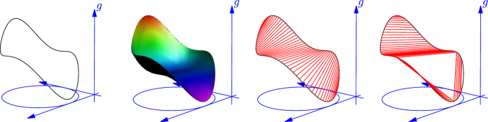
$g(\pi)$                   convex extension        $\leq$            roof extension                  largest convex ext. = smallest roof ext. = convex roof

Figure 1: An illustration of the convex roof extension where $\Omega$ is a disc and $\partial_{e}\Omega$ a circle.

Fig. 1 may illustrate the concept and explain the name. In a roof extension, the ground floor $\Omega$ is covered by straight roof beams and plane tiles. Those beams and tiles rest with their ends on the the wall erected by $g(\pi)$. It is immediately clear from the definition of convexity that every convex extension is pointwise majorized by every roof extension. But is the largest convex extension a roof? The following theorem asserts that this is true at least when $g$ is continuous and $\Omega$ compact:

Theorem II.1 (Benatti et al. (1996); Uhlmann (1998)).

Let $g(\pi)$ be a continuous real-valued function on the set of pure states $\partial_{e}\Omega$. There exists exactly one function $g^{\cup}(\omega)$ on $\Omega$ which can be characterized uniquely by each one of the following four properties:

1. $g^{\cup}$ is the unique convex roof extension of $g$.

2. $g^{\cup}(\omega)$ is the solution of the optimization problem

   $$g^{\cup}(\omega)=\inf_{\omega={}^{c}\sum p_{j}\,\pi_{j}}\;\sideset{{}^{c}}{}{\sum}p_{j}\,g(\pi_{j}).$$ (9)

3. $g^{\cup}(\omega)$ is largest convex extension as well as the smallest roof extension of $g$.

Furthermore, given $\omega\in\Omega$, the function $g^{\cup}$ is convex-linear on the convex hull of all pure states $\pi$ appearing in optimal decompositions of $\omega$.

Therefore, $g^{\cup}$ provides a foliation of $\Omega$ into compact leaves such that a) each leaf is the convex hull of some pure states and b) $g^{\cup}$ is convex-linear on each leaf.

Remark II.1.

1. The theorem justifies to write “min” instead of “inf” in Eqs. (1) and (9).

2. If $g^{\cup}$ is not only linear but even constant on each leaf, it is called a flat roof.

3. Let $f(\omega)$ be a concave function on $\Omega$, e.g., $f(\omega)=S(\Phi(\omega))$. Then we denote by $f^{\cup}$ the convex roof extension of $f|_{\partial_{e}\Omega}$.

III Symmetries and invariant states

The following lemma gives a simple bound for $f^{\cup}$. Let $P:\Omega\rightarrow\Xi$ be an affine and surjective map $\omega\mapsto\xi$. The space $\Xi$, as the image of $\Omega$ under an affine map, is convex and compact, but it need not be a quantum state space. The map $P$ provides a foliation of $\Omega$ into leaves $\Omega=\bigcup_{\xi\in\Xi}L_{\xi}$ via

$$L_{\xi}=\{\omega\,|\,\omega\in\Omega,P(\omega)=\xi\}.$$ (10)

Since $P$ is affine, every leaf is generated by cutting $\Omega$ with some hyperplane and therefore, the leaves are convex, too. We define the function $\epsilon(\xi)$ on $\Xi$ as the minimum of $f$ on the corresponding leaf

$$\epsilon(\xi)=\min_{L_{\xi}}f(\omega)=\min\{f(\omega)\,|\,P\omega=\xi\}.$$ (11)

Lemma III.1.

The convex hull of the $\epsilon$ function, $\epsilon^{\Cup}(\xi),$ provides a lower bound for the convex roof $f^{\cup}(\omega)$, i.e.,

$$f^{\cup}(\omega)\geq\epsilon^{\Cup}(P\omega)$$ (12)

Proof.

Let $\omega=\sum\lambda_{i}\omega_{i}$ be optimal for $f^{\cup}$, so $f^{\cup}(\omega)=\sum\lambda_{i}f(\omega_{i})$. Let $\xi_{i}=P\omega_{i}$. Then, due to linearity of $P$ we have $\xi=\sum\lambda_{i}\xi_{i}$ and due to the definition of $\epsilon(\xi)$ we have $f(\omega_{i})\geq\epsilon(\xi_{i})$. So,

$$f^{\cup}(\omega)=\sum\lambda_{i}f(\omega_{i})\geq\sum\lambda_{i}\epsilon(\xi_{i})$$ (13)

and from eq. (5), we have

$$\sum\lambda_{i}\epsilon(\xi_{i})\geq\epsilon^{\Cup}(\xi).$$ (14)

∎

There are some cases where we can find states $\omega$ for which the inequality of the lemma can be sharpened to an equality.

Theorem III.2.

Let $P=P^{2}$ be a linear and idempotent map of the state space onto itself with an fixed point set $P\Omega=\Xi\subset\Omega$ of $P$-invariant states. Let $f(\omega)$ be $P$-invariant,i.e.,

$$f(P\omega)=f(\omega)\quad\forall\omega\in\Omega$$ (15)

Then for all $P$-invariant states $\omega_{P}\in P\Omega$ holds

$$f^{\cup}(\omega_{P})=\epsilon^{\Cup}(\omega_{P})=\epsilon^{\cup}(\omega_{P})$$ (16)

and these states have an optimal decomposition completely in $P\Omega$, i.e., into $P$-invariant states only. Furthermore, for every state $\omega$ it holds that

$$f^{\cup}(\omega)\geq f^{\cup}(P\omega)$$ (17)

Proof.

Since $f$ is $P$-invariant, it is constant on every affine subspace $P^{-1}\omega$. Therefore, we have $\epsilon(\omega)=f(\omega)$ on $P\Omega$ and $\epsilon$ is concave. So, $\epsilon^{\Cup}(\omega)=\epsilon^{\cup}(\omega)$. Let $\omega={}^{c}\sum\lambda_{j}\omega_{j}$ be optimal for $\epsilon^{\cup}$. Then,

$$\epsilon^{\cup}(\omega)=\sideset{{}^{c}}{}{\sum}\lambda_{j}\epsilon(\omega_{j})=\sideset{{}^{c}}{}{\sum}\lambda_{j}f(\omega_{j})\geq f^{\cup}(\omega).$$ (18)

Together with Lemma III.1 this proves (16) and provides an $f^{\cup}$-optimal decomposition lying in $P\Omega$. ∎

Example III.1.

Let $P$ be the projection to real states $P(\omega)=1/2(\omega+\omega^{\top})$ and $f$ the output entropy of the diagonal map $S^{D}_{\text{out}}(\omega)=S(\Phi_{D}(\omega))$. Then real states have optimal decompositions into real states only. Furthermore, Lemma III.1 asserts that all non-real states have an entanglement entropy at least as large as their real projections

$$E_{D}(\omega)=f^{\cup}(\omega)\geq\epsilon^{\cup}(P\omega)=E_{D}(P\omega)\qquad\forall\omega\in\Omega$$ (19)

A slightly different version was used in Terhal and Vollbrecht (2000) and worked out in Vollbrecht and Werner (2001):

Theorem III.3 (Terhal and Vollbrecht (2000); Vollbrecht and Werner (2001)).

Let $G$ be a symmetry goup of $f$ such that $f(\omega^{g})=f(\omega)$ for all $\omega\in\Omega$ and $g\in G$. Let $P_{G}$ be the twirl map or group average corresponding to $G$, i.e., the idempotent projection to the subspace $P_{G}\Omega$ of $G$-invariant states

$$\omega_{P}=P_{G}\omega=\frac{1}{|G|}\sum_{g\in G}\omega^{g}$$ (20)

Then for all $G$-invariant states $\omega_{P}\in P_{G}\Omega$ holds

$$f^{\cup}(\omega_{P})=\epsilon^{\Cup}(\omega_{P}).$$ (21)

Furthermore, for every state $\omega\in\Omega$ it holds that

$$f^{\cup}(\omega)\geq f^{\cup}(P\omega)$$ (22)

States $\omega_{P}$ for which $\epsilon^{\Cup}(\omega_{P})=\epsilon(\omega_{P})$ have an optimal decomposition consisting of one complete orbit of $G$; otherwise the optimal decomposition consists of several complete orbits.

Proof.

We assume that $\omega_{P}=\sum\lambda_{i}\omega_{i}$ is optimal for $\epsilon^{\Cup}(\omega_{P})$. Let $\tilde{\omega}_{i}$ be states which achieve the minimum in eq. (11) for the $\omega_{i}$: $\epsilon(\omega_{i})=f(\tilde{\omega}_{i})$ and $\tilde{\omega}_{i}$ belongs to the leaf $L_{i}$. So, $P\tilde{\omega}_{i}=\omega_{i}$ and therefore

$$\omega_{P}=\sum_{i,g}\frac{\lambda_{i}}{|G|}\;\tilde{\omega}^{g}_{i}$$ (23)

is a candidate decomposition for $f$. So,

$$f^{\cup}(\omega_{P})\leq\sum_{i,g}\frac{\lambda_{i}}{|G|}\;f(\tilde{\omega}^{g}_{i})$$ (24)

With $f(\omega^{g})=f(\omega)$ and $\sum_{g}\frac{1}{|G|}=1$, the right hand side evaluates to

$$f^{\cup}(\omega_{P})\leq\sum_{i}\lambda_{i}f(\tilde{\omega}_{i})=\sum\lambda_{i}\epsilon(\omega_{i})=\epsilon^{\Cup}(\omega)$$ (25)

This, together with lemma III.1, proves the theorem and shows that decomposition (23) is optimal for $f^{\cup}$. ∎

Please note that the $G$-invariance of $f$ does not imply $P_{G}$-invariance of $f$. This is the main difference between Theorem III.2 and Theorem III.3 for applications.

Only in the case where $f(\omega)$ is $P_{G}$-invariant $f(P\omega)=f(\omega)$ (which implies $G$-invariance $f(\omega^{g})=f(\omega)$) we know that every $G$-invariant state has an optimal decomposition consisting solely of $G$-invariant states.

IV Output entropy of the diagonal map

The diagonal map $\Phi_{D}$ maps $\Omega_{N}$, the state space of an $N$-dimensional Hilbert space, to the simplex $\Omega^{\prime}_{N}=\{x_{1},x_{2},...,x_{N}\},$ $\;0\leq x_{i}\leq 1,$ $\sum x_{i}=1$. It corresponds to a complete von Neumann measurement. Its Kraus form is

$$\Phi(\omega)=\sum_{i=1}^{N}\;P_{i}\omega P_{i}$$ (26)

with $P_{i}=|i\rangle\langle i|$. The output entropy of this channel is

$$S_{\text{out}}^{D}(\omega) =S(\Phi_{D}(\omega))$$ (27)

$$=\sum_{i=1}^{N}\eta(x_{i})$$ (28)

with the usual abbreviation $\eta(x)=-x\log(x)$ for $x>0$ and $\eta(0)=0$. This function is not only concave but a concave roof, as was shown in Uhlmann (2010).

The minimal output entropy is zero and the maximal one is $\log N$.

Things become more refined by restricting the channel onto a face of $\Omega_{N}$. As an example we take the $(N-1)$-dimensional subspace $\mathcal{H}_{0}$ which is orthogonal to the vector $|\phi\rangle=N^{-1/2}\sum|j\rangle$. It consists of vectors $\sum a_{j}|j\rangle$ such that $\sum a_{j}=0$. $\mathcal{H}_{0}$ supports pure states satisfying $\Phi_{D}(\pi)=N^{-1}\mathbbm{1}$ and so the maximal output entropy is $\log N$ again.

For the minimal output entropy we have a more complex result:

Theorem IV.1.

Let $\Omega_{0}$ be the face of $\Omega_{N}$ consisting of states whose support is orthogonal to $\sum_{i=1}^{N}|i\rangle$. Let $S_{\text{min}}^{D}$ be the minimal output entropy of the diagonal map $\Phi_{D}$. Then we have:

• We have $S_{\text{min}}^{D}(\Omega_{0})=\log 2$ for For $N=2,3,\dots 6$. This is achieved by the $N(N-1)/2$ pure input states $\pi_{jk},\;j<k$, and only by these states. Here, $\pi_{jk}=|\phi_{jk}\rangle\langle\phi_{jk}|$ with $|\phi_{nm}\rangle=2^{-1/2}\left(|n\rangle-|m\rangle\right)$.

• For $N>6$ we have

  $$S_{\text{min}}^{D}(\Omega_{0})=\log N-\left(1-\frac{2}{N}\right)\log(N-1)$$ (29)

  and $\lim_{N\rightarrow\infty}S^{D}_{\text{min}}=0.$ The minimum is achieved by the $N$ states $\pi_{j}=|\phi_{j}\rangle\langle\phi_{j}|$ where

  $$\phi_{1}=\left(\,(N-1)a,\,-a,\,-a\,,...,-a\,\right)\qquad\text{ with }\qquad a=(N(N-1))^{-1/2}$$ (30)

  and the other $\phi_{i}$ are obtained by permuting the components.

The proof of this theorem is found in the appendix.

V Entanglement entropy of the $N=3$ diagonal map for some subsets of states

V.1 Geometry of the $N=3$ state space

The space $\Omega_{3}$ of positive hermitean $3\times 3$ matrices with unit trace has 8 real dimensions. Its boundary consists of zero-dimensional faces (pure states) and three-dimensional faces (Bloch balls), the latter corresponding to two-dimensional subspaces of the Hilbert space $\mathcal{H}=\mathbb{C}^{3}$.

We will use the notion $\psi=(a,b,c)$ to denote a one-dimensional subspace $[\mathbb{C}\psi]$ of $\mathbb{C}^{3}$ as well as the corresponding point $\pi_{\psi}=|\psi\rangle\langle\psi|$ of $\Omega_{3}$. Here, $(a,b,c)$ is a generally unnormalized element of this one-dimensional subspace. The set of states orthogonal to a given pure state $\psi$ form a Bloch ball which we denote by $B^{\perp}(\psi)$:

$$B^{\perp}(\psi):=\{\omega\,|\,\langle\psi|\omega|\psi\rangle=0\}$$ (31)

and all non-trivial faces of $\Omega_{3}$ are obtained in this way: There is a Bloch ball opposite to each pure state and this gives a bijection between the 0- and 3-dimensional faces of $\Omega$.

More generally, we can consider for every pure state $\psi$ the foliation of $\Omega_{3}$ by parallel hyperplanes $L_{\psi}(F)$ defined as

$$L_{\psi}(F):=\{\omega\,|\;\langle\psi|\omega|\psi\rangle=F\}$$ (32)

where $F$ is the fidelity parameter. The leaves are 7-dimensional in the generic case, but the highest leaf $L_{\psi}(1)=\pi_{\psi}$ consist of one pure state only and the lowest leaf $L_{\psi}(0)=B^{\perp}(\psi)$ is the Bloch ball opposite to $\psi$. Furthermore, every basis $\{\psi_{1},\psi_{2},\psi_{3}\}$ of three orthogonal pure states spans an equilateral triangle in $\Omega_{3}$. Every edge $\overline{\psi_{i}\psi_{j}}$ of this triangle is the diameter of the Bloch ball $B^{\perp}(\psi_{k})$ orthogonal to the opposite vertex, see Fig. 2.

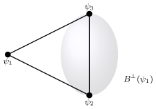
Figure 2: Bloch ball face and opposite face. Note that the plane of the triangle and the ball have only a one-dimensional intersection, the diameter $\overline{\psi_{2}\psi_{3}}$

All these triangles have the barycenter $\mathbbm{1}/3$ of $\Omega$ in common.

V.2 States of lowest entanglement entropy

The triangle spanned by the computational basis $\left(\begin{smallmatrix}1\\ 0\\ 0\end{smallmatrix}\right),\left(\begin{smallmatrix}0\\ 1\\ 0\end{smallmatrix}\right),\left(\begin{smallmatrix}0\\ 0\\ 1\end{smallmatrix}\right)$ is the lowest leaf of the roof of $E_{D}=S_{D}^{\cup}$, the leaf where $E_{D}=0$. Especially, $E(\mathbbm{1}/3)=0$. This triangle is the fixed point set of the diagonal channel $\Phi_{D}$.

V.3 Some rank-2 states

We can calculate $E_{D}$ for every Bloch ball which includes one of the three states of the computational basis. Take, for example, $B(\psi_{0},\psi_{ab})$, the ball spanned by $\psi_{0}=(1,0,0)$ and some orthogonal state $\psi_{ab}=(0,a,b)$. This ball is the image of the unitary embedding $V\colon\left(\begin{smallmatrix}1\\ 0\end{smallmatrix}\right)\mapsto\left(\begin{smallmatrix}1\\ 0\\ 0\end{smallmatrix}\right),\;\left(\begin{smallmatrix}0\\ 1\end{smallmatrix}\right)\mapsto\left(\begin{smallmatrix}0\\ a\\ b\end{smallmatrix}\right)$ of a standard Bloch ball. This embedding can be used to reduce the calculation of the convex roof to the $N=2$ case, see chapter 6.2 in Uhlmann (2010). Using the known results for the $N=2$ diagonal map (see, e.g., Benatti et al. (2003)) we find for states from this Bloch ball, i.e., states of the form

$$\omega=\begin{pmatrix}1-z&xa&xb\\ x^{*}a^{*}&z\,a^{*}a&z\,a^{*}b\\ x^{*}b^{*}&z\,ab^{*}&z\,b^{*}b\end{pmatrix}$$ (33)

with real $z$ and complex $x,a,b$ the entanglement entropy

$$E_{D}=\eta\left(\frac{1+\lambda}{2}\right)+\eta\left(\frac{1-\lambda}{2}\right)+z\,\eta(a^{*}a)+z\,\eta(b^{*}b)\quad\text{where}\quad\lambda=\sqrt{1-4x^{*}x}.$$ (34)

V.4 Real permutation invariant states

The permutation group $G=S_{3}$ acts on $\Omega_{3}$ by permuting the computational basis $\left\{\left(\begin{smallmatrix}1\\ 0\\ 0\end{smallmatrix}\right),\left(\begin{smallmatrix}0\\ 1\\ 0\end{smallmatrix}\right),\left(\begin{smallmatrix}0\\ 0\\ 1\end{smallmatrix}\right)\right\}$. The corresponding twirl acts on normalized pure states $\psi=(a,b,c)$ as

$$P_{G}(\pi_{\psi})=\frac{1}{3}\begin{pmatrix}1&z&z\\ z&1&z\\ z&z&1\end{pmatrix}\quad\text{where}\quad 2z=ab^{*}+a^{*}b+ac^{*}+a^{*}c+bc^{*}+b^{*}c.$$ (35)

Let us denote the $S_{3}$-invariant state on the right hand side as $\omega(z)$. In what follows, we restrict our considerations to real states $\omega=\omega^{\top}$. Then the real parameter $z$ can take values in the range

$$-\frac{1}{2}\leq z\leq 1.$$ (36)

Another often used parametrization for these states uses the fidelity with respect to the state $\omega(1)=\pi(1,1,1)$. We have

$$F=\langle\psi_{(1,1,1)}|\omega|\psi_{(1,1,1)}\rangle=\frac{1}{3}(2z+1).$$ (37)

The state $\omega(z)$ is of rank three except at the boundaries of the $z$ range:

• For $z=1$ we have a pure state

  $$\omega(1)=\pi(1,1,1)$$ (38)

  where we use $\pi(a,b,c)$ as shorthand for the pure state $\pi_{\psi}=|\psi\rangle\langle\psi|$ with $\psi\sim(a,b,c)$. So its entanglement entropy equals its output entropy and we have

  $$E_{D}(1)=\log(3).$$ (39)

• For $z=-\nicefrac{{1}}{{2}}$ we have a rank-2 state

  $$\omega(-\nicefrac{{1}}{{2}})=\frac{1}{2}\left[\pi(-1,0,1)+\pi(-1,2,-1)\right].$$ (40)

  This state belongs to the face of $\Omega$ considered in Section IV, so its entanglement entropy can’t be smaller than $\log(2)$. It is easy to see that this value can indeed be achieved by the optimal decomposition

  $$\omega\left(-\nicefrac{{1}}{{2}}\right)=\frac{1}{3}\left[\pi(1,0,-1)+\pi(0,-1,1)+\pi(-1,1,0)\right],$$ (41)

  and therefore

  $$E_{D}\left(-\nicefrac{{1}}{{2}}\right)=\log(2)$$ (42)

• Let’s also mention that for $z=0$ we have the maximally mixed state which belongs to the lowest leaf of Section V.2. So an optimal decomposition is

  $$\omega(0) =\frac{1}{3}\left[\pi(1,0,0)+\pi(0,1,0)+\pi(0,0,1)\right],$$ (43)

  $$E_{D}(0) =0.$$ (44)

Applying Theorem III.2 using the projection $P\omega=\frac{1}{2}(\omega+\omega^{\top})$ we see that the states $\omega(z)$ have optimal decompositions including only real states. Furthermore, for an arbitrary state we have

$$E_{D}(\omega)\geq E_{D}\left(\frac{\omega+\omega^{\top}}{2}\right).$$ (45)

Applying now Theorem III.3 with the projection $P_{G}$ to the space of real states we learn that

$$E_{D}(z)=\epsilon^{\Cup}(z)\quad\text{where}\quad\epsilon(z)=\min_{P_{G}(\pi(a,b,c))=\omega(z)}\;S_{D}\left(\pi(a,b,c)\right),\quad\text{with }z,a,b,c\text{ real}$$ (46)

The minimization in Eq. (46) is one-dimensional since the three real parameters are constrained by $a^{2}+b^{2}+c^{2}=1,$ $ab+bc+ac=z$. A useful parametrization of this constraint is Benatti et al. (1996)

$$3\,(a,b,c)=(\,\alpha+2\beta\cos\theta,\;\alpha-2\beta\cos(\theta-\pi/3),\;\alpha-2\beta\cos(\theta+\pi/3)\,)\quad\text{where}\quad\alpha=\sqrt{2z+1},\;\beta=\sqrt{1-z}$$ (47)

Numerical search for the minimum in Eq. (46) shows that the minimum is reached at $\theta=0$ for all $z>-0.4150234$. For smaller values of $z$, $\theta_{\text{min}}$ increase up to $\theta_{\text{min}}=\nicefrac{{\pi}}{{6}}$ at $z=-\nicefrac{{1}}{{2}}$. A thorough analysis of the function $\epsilon(z)$ obtained by this minimization shows that it is not everywhere convex. In the region $z\geq 0$ we re-obtained the result of Benatti et al. (2003): the convex hull $\epsilon^{\Cup}$ is obtained by replacing $\epsilon(z)$ in the region $\nicefrac{{5}}{{6}}<z\leq 1$ with a linear piece.

In the negative-$z$ region our results differ from Benatti et al. (2003), who claimed that $\epsilon(z)$ is convex there. We find that the convex hull is obtained by replacing $\epsilon(z)$ in the region between $z=-\nicefrac{{1}}{{2}}$ and $z=z^{*}=-0.4079496711$ with a linear piece, see Fig. 3.

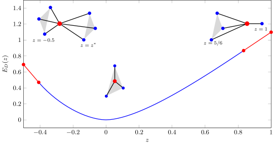
Figure 3: Entanglement entropy and optimal decompositions. Regions where the convex hull construction leads to a linear behaviour are drawn in red. The drawings indicate the shape of optimal decompositions of the red state into pure (blue) states in the three regions $z<z^{*},\;z^{*}\leq z<\nicefrac{{5}}{{6}},\;\nicefrac{{5}}{{6}}<z$, resp. Here, gray surfaces indicate hyperplanes of states which project under $P_{G}$ to the same value of $z$. The corners of the triangles form a complete orbit under the permutation group $G=S_{3}.$

Interestingly, everywhere in the region $z^{*}\leq z\leq\nicefrac{{5}}{{6}}$ where $\epsilon(z)=\epsilon^{\Cup}(z)$ the minimum is obtained for states with $\theta=0$. So the optimal decompositions in this region have the form

$$\omega=\frac{1}{3}\left[\pi(a,b,b)+\pi(b,b,a)+\pi(b,a,b)\right],$$ (48)

corresponding to a short orbit of $S_{3}$ of length 3 only. In the region $-\nicefrac{{1}}{{2}}<z<z^{*}$ the optimal decomposition has length 6 and is a mixture of two such short orbits resulting in a large region in state space where the entanglement entropy is an affine function.

With

$$\mathcal{S}(z)=2\eta\left(\frac{(\alpha-\beta)^{2}}{9}\right)+\eta\left(\frac{(\alpha+2\beta)^{2}}{9}\right)\quad\text{where}\quad\alpha=\sqrt{2z+1},\;\beta=\sqrt{1-z}$$ (49)

and $z^{*}=-0.4079496711$, $\mathcal{S}(\nicefrac{{5}}{{6}})=\log(3)-\nicefrac{{1}}{{3}}\log(2)$ the final result for the entanglement entropy is therefore

$$E_{D}(z)=\begin{cases}p\log(2)+(1-p)\mathcal{S}(z^{*})&\text{for }-\nicefrac{{1}}{{2}}\leq z<z^{*}\text{ with }p=\frac{z^{*}-z}{z^{*}+\nicefrac{{1}}{{2}}}\\ \quad\mathcal{S}(z)&\text{for }z^{*}\leq z\leq\nicefrac{{5}}{{6}}\\ p[\log(3)-\nicefrac{{1}}{{3}}\log(2)]+(1-p)\log(3)&\text{for }\nicefrac{{5}}{{6}}<z\leq 1\text{ with }p=\frac{1-z}{1-\nicefrac{{5}}{{6}}}\end{cases}$$ (50)

Appendix A Proof of theorem IV.1

1. We have $S^{D}_{\text{out}}(\omega)=S^{D}_{\text{out}}(\omega^{\top})=S^{D}_{\text{out}}(\frac{1}{2}(\omega+\omega^{\top}))$. Therefore we can restrict our search for the minimum to the subspace $\Omega_{\mathbb{R}}=\{\omega\;|\;\omega=\omega^{\top}\}$ of real states.

2. The minimal output entropy is attained by pure states since $S_{\text{out}}^{D}$ is concave and $\Omega_{\mathbb{R}}$ is convex.

3. The case $N=2$ is trivial. There is only one pure real state $\phi_{12}=\phi_{1}=2^{-1/2}(1,-1)$ in $\mathcal{H}_{0}$ with $S_{\text{out}}^{D}=\log 2$. So we now assume $N\geq 3$.

4. The pure real states in $\mathcal{H}_{0}$ have the form $\pi=|\psi\rangle\langle\psi|$ with

   $$|\psi\rangle=\sum a_{j}|j\rangle,\qquad\sum a_{j}=0,\qquad\sum a_{j}^{2}=1\qquad\text{which implies}\qquad a_{i}\in(-1,1).$$ (51)

   So we use Lagrange’s multiplier method to find the minimum of

   $$S_{\text{out}}^{D}(\pi)=-\sum a_{j}^{2}\log a_{j}^{2}$$ (52)

   for all $a_{i}$ satisfying eq. (51). The equations to solve read

   $$a_{i}\log a_{i}^{2}+a_{i} =\lambda+a_{i}\mu^{\prime}$$ (53)

   $$\text{ or: }\quad\qquad a_{i}\log a_{i}^{2} =\lambda+a_{i}\mu\qquad$$ (54)

   where $\lambda,\mu^{\prime}$ denote Lagrange multipliers for the constraints Eq. (51) and $\mu=\mu^{\prime}-1$. Multiplying eq. (54) by $a_{j}$ and summing over $j$ yields

   $$S_{\text{out}}^{D}=-\mu\qquad\text{and therefore,}\qquad\mu<0.$$ (55)

   Not all solutions of eq. (54) have minimal output entropy but all states of minimal entropy must be solutions of eq. (54). So can find the minimum by classifying all solutions and comparing their entropy. Let us consider different cases:

   1. $\lambda=0$, so the solutions of eq. (54) are $a_{i}\in\{0,\pm\exp(\mu/2)\}$. Let $m$ instances of the $a_{i}$ be nonzero. Then their modulus must be $m^{-1/2}$ for $\sum a_{j}^{2}=1$ and $S_{\text{out}}^{D}=-\mu=\log m$. Since $m$ must be even for $\sum a_{j}=0$, the minimum value for $S_{D}$ is achieved for $m=2$. So one candidate for the minimum of $S_{\text{out}}^{D}$ is

      $$S_{\text{out}}^{D}=\log 2,\qquad|\phi_{jk}\rangle=2^{-1/2}\left(|j\rangle-|k\rangle\right)$$ (56)

   2. $\lambda\neq 0$. Then all the $a_{i}$ have to be non-zero. The transcendental equation $\lambda+x\mu=x\log x^{2}$ can be rewritten as

      $$\frac{\lambda}{2}e^{-\frac{\mu}{2}}=\frac{\lambda}{2|x|}e^{\frac{\lambda}{2x}}=\pm we^{w}\quad\text{with}\quad w=\lambda/2x$$ (57)

      The inverse of the function $f(w)=we^{w}$ is the Lambert $W$ function $W(z)$Corless et al. (1996), defined via

      $$z=W(x)\;e^{W(z)}.$$ (58)

      As an inverse of a non-injective function it has multiple branches, two of which are real and denoted as $W_{-1}$ and $W_{0}$. It follows that $\lambda+\mu x=x\log x^{2}$ has no more than three real solutions which can be expressed as

      $$x_{1} =\frac{\lambda}{2W_{0}(z)}\quad\text{where}\quad z=\frac{|\lambda|}{2}e^{-\mu/2}$$ (59)

      $$x_{2} =\frac{\lambda}{2W_{0}(-z)}$$ (60)

      $$x_{3} =\frac{\lambda}{2W_{-1}(-z)}$$ (61)

      Since $\lambda\neq 0$ we have $z>0$. Then a solution $x_{1}$ does always exist and the solutions $x_{2}$ and $x_{3}$ exist only if $z\leq 1/e$. They are equal for $z=1/e$.

      1. Let us assume that only two of the values, say $x_{1}$ and $x_{2}$ are used in the state. So we have

         $$nx_{1}+mx_{2}=0,\quad nx_{1}^{2}+mx_{2}^{2}=1,\quad n+m=N,\quad n,m\geq 1$$ (62)

         resulting in $x_{1}^{2}=\frac{m}{nN},\;\;x_{2}^{2}=\frac{n}{mN}$ and so

         $$S(N,n)=\log N-\left(1-\frac{2n}{N}\right)\log\left(\frac{N}{n}-1\right)$$ (63)

         Now this expression is concave in $n$:

         $$\frac{\partial^{2}S(N,m)}{\partial n^{2}}=-\frac{N^{2}}{n^{2}(N-n)^{2}}<0\quad\text{for}\quad 0<n<N$$ (64)

         and therefore takes for fixed $N$ its minimum at the edges of the allowed $n$-range, $n=1$ or, equivalently, $n=N-1$.

         So the second possibility for a minimum of $S_{\text{out}}^{D}$ is

         $$S_{\text{out}}^{D}=\log N-\left(1-\frac{2}{N}\right)\log\left(N-1\right),\qquad\{a_{j}\}=(a,a,...,a,(1-N)a)$$ (65)

      2. The last possibility is that all three roots $x_{1},x_{2},x_{3}$ occur among the $a_{i}$. Consider the function

         $$F(\lambda,\mu)=x_{1}^{2}+x_{2}^{2}+x_{3}^{2}$$ (66)

         where the $x_{i}$ are the three solutions of $\lambda+\mu x=x\log x^{2}$. Using Eqs. (58,59,60,61) we find

         $$F(\lambda,\mu) =e^{\mu}\left(e^{2W_{0}(z)}+e^{2W_{0}(-z)}+e^{2W_{-1}(-z)}\right)$$ (67)

         $$=e^{\mu}G(\lambda,\mu)$$ (68)

         $$\text{where}\qquad G(\lambda,\mu) =e^{2W_{0}(z)}+e^{2W_{0}(-z)}+e^{2W_{-1}(-z)}$$ (69)

         

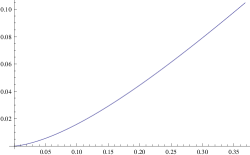
         Figure 4: Plot of $G^{\prime}(z)$ over $z$

         Now we have $G(0)=2$ and $G^{\prime}(z)>0$ for $z\in(0,1/e]$ (see Fig. 4), therefore $G(z)>2$ for $z\in(0,1/e]$. Since we need $F\leq 1$ for a normalized state vector, this implies $e^{\mu}<\frac{1}{2}$, $\mu<-\log 2$, $S^{D}_{\text{out}}=-\mu>\log 2$ and therefore any such solution has larger output entropy than the state given by Eq. (56).

5. The only thing left to do is to compare the two candidates for a minimum, Eqs. (65) and (56). It is easy to see, that candidate (56)

   

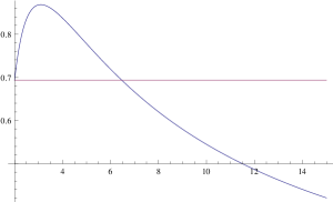
   Figure 5: The output entropies $\log 2$ and Eq. (65) plotted over $N$

   wins for $N\leq 6$ and candidate (65) wins for all $N>6$, see Fig. 5. $\square$

References

- Bennett et al. (1996) C. H. Bennett, D. P. DiVincenzo, J. A. Smolin, and W. K. Wootters, Physical Review A 54, 3824 (1996), eprint quant-ph/9604024.
- Schumacher and Westmoreland (1997) B. Schumacher and M. D. Westmoreland, Phys. Rev. A 56, 131 (1997).
- Holevo (1998) A. S. Holevo, IEEE Transactions on Information Theory 44, 269 (1998), quant-ph/9611023.
- Benatti et al. (1996) F. Benatti, H. Narnhofer, and A. Uhlmann, Rep. Math. Phys 38, 123 (1996).
- Connes et al. (1987) A. Connes, H. Narnhofer, and W. Thirring, Commun. in Math. Phys. 112, 691 (1987).
- Benatti (2009) F. Benatti, Dynamics, Information and Complexity in Quantum Systems (Springer, 2009).
- Terhal and Vollbrecht (2000) B. M. Terhal and K. G. H. Vollbrecht, Phys. Rev. Lett. 85, 2625 (2000).
- Vollbrecht and Werner (2001) K. G. H. Vollbrecht and R. F. Werner, Phys. Rev. A 64, 062307 (2001), eprint quant-ph/0010095.
- Manne and Caves (2008) K. K. Manne and C. M. Caves, Quantum Information & Computation 8, 295 (2008).
- Wootters (1998) W. K. Wootters, Phys. Rev. Lett. 80, 2245 (1998), eprint quant-ph/9709029.
- Benatti et al. (1999) F. Benatti, H. Narnhofer, and A. Uhlmann, Lett. Math. Phys. 47 (1999).
- Benatti et al. (2003) F. Benatti, H. Narnhofer, and A. Uhlmann, J. Math. Phys. 44, 2402 (2003).
- Uhlmann (1998) A. Uhlmann, Open Sys. Information Dyn. 5, 209 (1998), eprint quant-ph/9701014.
- Uhlmann (2010) A. Uhlmann, Entropy 12, 1799 (2010).
- Corless et al. (1996) R. Corless, G. Gonnet, D. Hare, D. Jeffrey, and D. Knuth, Adv. in Computational Math. 5, 329 (1996).