Random degree-degree correlated networks

Abstract

Correlations may affect propagation processes on complex networks. To analyze their effect, it is useful to build ensembles of networks constrained to have a given value of a structural measure, such as the degree-degree correlation $r$, being random in other aspects and preserving the degree sequence. This can be done through Monte Carlo optimization procedures. Meanwhile, when tuning $r$, other network properties may concomitantly change. Then, in this work we analyze, for the $r$-ensembles, the impact of $r$ on properties such as transitivity, branching and characteristic path lengths, that are relevant when investigating spreading phenomena on these networks. The present analysis is performed for networks with degree distributions of two main types: either localized around a typical degree (with exponentially bounded asymptotic decay) or broadly distributed (with power-law decay). Size effects are also investigated.

I Introduction

Complex networks are realistic substrates for simulating many social and natural phenomena. To address the influence of network topology, primarily, different classes of degree distributions $P(k)$ can be considered. Meanwhile, for a given distribution of degrees, correlations may give rise to important network structure effects on the studied process vazquez ; small ; optimizing ; epidemic ; makse ; threshold . These structural effects may have important consequences, for instance, correlations may shift the epidemic threshold threshold . Although correlation effects may be absent in some cases absence , in other ones, they can not be neglected.

Despite there are efficient algorithms to generate networks with fixed degree-degree correlations pusch , real joint probabilities of two or more degrees measured in networks of moderate size may be noisy and hard to be modeled. Then, operationally, average nearest-neighbors degree distributions asymptotic or single quantity measures are used. Although other variants have been defined in the literature mixing ; reshuffling , as quantifier of the tendency of adjacent vertices to have similar or dissimilar degrees, we will consider the standard measure of (linear) degree-degree correlations, namely, the assortativity (Pearson) coefficient newman_assor

$$r=\frac{\langle kk^{\prime}\rangle_{e}-\langle k\rangle^{2}_{e}}{\langle k^{2}\rangle_{e}-\langle k\rangle^{2}_{e}},$$ (1)

where $\langle\cdots\rangle_{e}$ denotes average over edges and $k$ and $k^{\prime}$ are the degrees of vertices at each end of an edge. Despite this coefficient is known to present some drawbacks cap3 , it is a standard and commonly used quantity, hence being worth to be analyzed. Moreover, it has the advantage of being a single value measure, that is easier to be controlled than other multi-valued quantities.

To analyze the influence of correlations, as well as of any other structural feature, it is useful to build ensembles of networks holding that property, while keeping fixed the sequence of degrees. As it will be described in Sec. II, this kind of ensembles can be achieved by means of a suitable rewiring, performed through a standard simulated annealing Monte Carlo (MC) procedure to minimize a given energy-like quantity (maximum entropy ensemble approach), function of the graph property to be controlled ($r$ in our case) park ; foster ; noh . Once tuned $r$, it is important to characterize how other network properties are altered as by product. Some interdependencies among certain network properties have already been numerically shown in the literature, for real as well as for artificial graphs foster . Analytical relations have also been derived estrada ; serrano2 ; dorogovtsev . Because of its crucial role in spreading phenomena newman2001 , we will focus here on the effect of $r$ over typical distance measures as well as on the branching and transitivity of links.

As a measure of the average separation between nodes, we consider the average path length WS . In the subsequent calculations we use the expression,

$$L=\frac{\sum_{i=1}^{n}\langle L_{i}\rangle N_{i}(N_{i}-1)}{\sum_{i=1}^{n}N_{i}(N_{i}-1)}\,,$$ (2)

where $n$ is the number of (disconnected) clusters and $N_{i}$ is the number of nodes in cluster $i$. Moreover, being $d_{kj}$ the distance (number of edges along the shortest path) between nodes $k$ and $j$ (taking $d_{kj}=0$ if the nodes do not belong to the same cluster), then

$$\langle L_{i}\rangle=\frac{\sum_{j,k=1}^{N_{i}}d_{kj}}{N_{i}(N_{i}-1)}\,.$$ (3)

Alternatively, in order to avoid the issue of the divergence of the distance between disconnected nodes, we consider the inverse, $1/E$, of the so-called efficiency latora

$$E=\frac{1}{N(N-1)}\sum_{\begin{subarray}{c}1\leq i,j\leq N\\ i\neq j\end{subarray}}\frac{1}{d_{ij}}\,,$$ (4)

where $N$ is the number of nodes. It represents a harmonic mean instead of the arithmetic one. We also compute the diameter $D=\mbox{max}\{d_{ij}\}$.

The transitivity of links can be measured by the clustering coefficient barrat ; newman_clus

$$C=\frac{6n_{\triangle}}{\sum_{i=1}^{N}k_{i}(k_{i}-1)}\,,$$ (5)

where $n_{\triangle}$ is the number of triangles and $k_{i}$ is the degree of node $i$. We also considered the mean value, $\bar{C}$, of the local clustering coefficient $C_{i}$, defined as $C_{i}=2e_{i}/(k_{i}(k_{i}-1))$, where $e_{i}$ is the number of connections between the neighbors of vertex $i$ WS . We took $C_{i}=0$ when $k_{i}=0$ or 1. Other measures that arise in the decomposition of $r$ estrada will also be considered.

Besides detecting interdependencies among structural properties, it is also important to know how these properties depend on the system size $N$. We will analyze these issues for two main classes of degree distributions (Poisson and power-law tailed). We will also investigate real networks degree sequences.

II Networks and ensembles

For each class of networks, we will consider different values of the size, $N$, and the mean degree, $\langle k\rangle$, within realistic ranges.

As a paradigm of the class of networks with a peaked distribution of degrees, with all its moments finite, we consider the random network of Erdős and Rényi ER . Within this model, a network with $N$ nodes is assembled by selecting $M$ different pairs of nodes at random and linking each pair. The resulting distribution of links is the Poisson distribution $P(k)=e^{-\langle k\rangle}\langle k\rangle^{k}/k!$, where the mean degree is $\langle k\rangle=2M/N$.

We also analyze networks of the power-law type, i.e., with $P(k)\sim k^{-\gamma}$, $\gamma>2$, corresponding to a wide distribution of degrees, with power-law tails. Then, moments of order $n\geq\gamma-1$ are divergent. We built power-law networks by means of the configuration model CM . Following this procedure, one starts by choosing $N$ random numbers $k$, drawn from the degree distribution $P(k)$. They represent the number of edges coming out from each node, where these edges have one end attached to the node and another still open. Second, two open ends are randomly chosen and connected such that, although multiple connections are allowed, self connections are not. This second stage is repeated until each node attains the connectivity attributed in the first step. If eventually an edge has an open end, then it is discarded. However, for large networks, the fraction of discarded edges is negligible. To draw the set of numbers $k$ with probability $P(k)={\cal N}k^{-\gamma}$, with $k_{min}\leq k\leq k_{max}$ (hence the normalization factor is ${\cal N}=1/\sum_{k_{min}}^{k_{max}}k^{-\gamma}$), we used the inverse transform algorithm transform . Notice that $k_{max}\leq N-1$ and $k_{max}>>k_{min}$, then we determined $k_{min}$ to fit the selected value of $\langle k\rangle$ (within a tolerance of at most 1%), such that

$$\langle k\rangle=\frac{\sum_{k_{min}}^{k_{max}}k^{-\gamma+1}}{\sum_{k_{min}}^{k_{max}}k^{-\gamma}}\simeq\frac{\gamma-1}{\gamma-2}\,\frac{k_{max}^{2-\gamma}-k_{min}^{2-\gamma}}{k_{max}^{1-\gamma}-k_{min}^{1-\gamma}}\simeq\frac{\gamma-1}{\gamma-2}k_{min}.$$ (6)

It is worth mentioning that the value $k=N-1$ is not usually achieved, the natural cut-off being $k_{c}\sim N^{\frac{1}{\gamma-1}}$ Dorogovtsev_cutoff .

In order to attain a desired value of $r$, we follow an standard rewiring approach. We want to build an ensemble of networks {G} with a given value of $r$ ($r$-ensemble) but that are maximally random in other aspects, i.e., making the fewer number of assumptions as possible about the distribution $P(G)$. Then, we use an exponential random graph model, such that the set of networks {G} has distribution $P(G)\propto{\rm e}^{-H(G)}$, where $H(G)$ is a Hamiltonian or energy-like quantity park . In order to get an $r$-ensemble, with $r=r_{\star}$, we consider foster

$$H(G)=\beta|r-r_{\star}|\,,$$ (7)

where $\beta$ is a real parameter. The ensemble can be simulated by means of a MC procedure: at each step, a rewiring attempt is accepted with probability $\mbox{min}\{1,e^{-[H(G^{\prime})-H(G)]}\}$. Rewiring steps are performed by randomly selecting two edges that connect the vertices $a$, $b$ and $c$, $d$, respectively, and substituting those two links by new ones connecting $a$, $c$ and $b$, $d$ rewiring . Movements yielding double links are forbidden. Notice that this process preserves the connectivity of each node. We start the simulation by taking $\beta=0$ [during at most 100 MC steps (MCS), where each MCS corresponds to $N$ attempts]. The effect of this stage is basically to destroy multiple edges. We did not notice any clear hysteresis effect like those observed when controlling, instead, the number of triangles with a differente Hamiltonian hysteresis . Subsequently, $\beta$ is increased (in increments $\Delta\beta=1000$), at each 50 MCS, until $r$ stabilizes, typically attaining the prescribed value $r_{\star}$. Then, the quantities of interest are calculated and the whole process is repeated, starting with a new degree sequence. For power-law degree distributions, we observed that the process is non-ergodic, hence we computed sample mean and standard deviation over 100 realizations of the described protocol. We checked that the choice of other expressions for $H(G)$, vanishing at $r_{\star}$, did not significantly affect the results but just the convergence time.

III Results

Let us start by reporting the effects of $r$ on the clustering coefficient $C$.

For the Poisson case, we depict in Fig. 1(a) the behavior of $C$ as a function of $r$ for a fixed number of nodes ($N=8000$) and different values of the mean connectivity $\langle k\rangle$. Very small values of $C$ emerge. The transitivity $C$ monotonically increases with $r$. This is consistent with the results of Ref. foster (restricted to $r\geq 0$) for such kind of networks. We observe two regimes with a crossover at $r\simeq 0.5$: a very slight increase with $r$ below the crossover and a more pronounced one in the region above it. The existence of two regimes could be related to the assymetric character of $r$, which does not measure assortativity and disassortativity on the same grounds. Below the crossover, $C$ linearly increases with $\langle k\rangle$ about one order of magnitude within the analyzed range. Meanwhile, above the crossover, $C$ remains of the same order when the average connectivity increases, even for small $\langle k\rangle$ (also see the inset of Fig. 1(a) where $C$ is plotted vs $\langle k\rangle$ for selected values of $r$). In Sec. IV, we will discuss these issues in more detail. For the mean local clustering coefficient $\bar{C}$, we obtained a qualitatively similar dependence on $r$ than that observed for the clustering coefficient $C$. However, the increase of $\bar{C}$ with $\langle k\rangle$ is linear for any fixed $r$. For $r=0$, $C=\bar{C}=\langle k\rangle/N$, as expected.

In Fig. 1(b), size effects are exhibited for $\langle k\rangle=4$, representative of the other values considered. As the number of nodes increases, $C$ decays as $C\sim 1/N$ for all $r$ (as depicted in the inset). Therefore, in the $r$-ensemble of Poisson networks, transitivity is only a finite-size effect and vanishes in the infinite network (thermodynamic) limit with the same asymptotic law $C\sim 1/N$ that for an uncorrelated random graph APC .

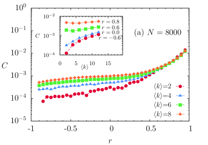
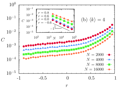
Figure 1: Clustering coefficient $C$ as a function of $r$ for Poisson networks: (a) $N=8000$ and different values of $\langle k\rangle$ indicated on the figure. The graph shows a monotonic increase of $C$ with $r$. There are two regimes: a very slight increase of $C$ with $r$ below $r\simeq 0.5$ and a more pronounced one above it. (b) $\langle k\rangle=4$ and different number of nodes $N$, also indicated on the figure. As the number of nodes increases, $C$ decays with the asymptotic law $C\sim 1/N$, characteristic of uncorrelated random graphs. Standard errors are about 10%. Dotted lines are a guide to the eyes. The insets show $C$ vs $\langle k\rangle$ (a) and $N$ (b) for selected values of $r$ (-0.6, 0.0, 0.6 and 0.8).

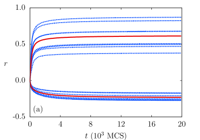
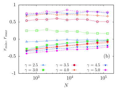
Figure 2: The range of allowed values of $r$ is restricted for the power-law class: (a) Time evolution of $r$, after setting $r_{\star}=1$ (-1) to obtain $r_{max}$ ($r_{min}$), for networks with power-law degree distribution (with $\gamma=3.5$ and $N=5000$). Shown are 8 individual samples (thin lines) and their respective averages (thick lines). (b) Average extreme values [$r_{max}$ (open symbols) and $r_{min}$ (filled symbols), standard errors are at most 50%] vs system size $N$ for different values of $\gamma$ indicated on the figure. Dotted and dashed lines are guides to the eye for $r_{max}$ and $r_{min}$, respectively. In all cases $\langle k\rangle=4.00\pm 0.04$. For a given size, the allowed interval of $r$ is narrower for lower $\gamma$.

For the power-law class, the range of allowed values of $r$ is restricted. That is, values of $r$ arbitrarily different from zero can not be attained in typical realizations of the MC protocol described in Sec. II. In order to determine the typical maximal (minimal) values, $r_{max}$ ($r_{min}$), we imposed $r_{\star}=1$ (-1) and detected the stationary values of $r$. The time evolution of $r$ for $r_{\star}=1$ (-1) is illustrated in Fig. 2(a) for $\gamma=3.5$, $N=5000$ and $\langle k\rangle\simeq 4$. Notice the large deviations amongst the steady values of different realizations mainly for the upper bound. We verified that this picture does not change by implementing other definitions of $H(G)$ in Eq. (7), e.g., $\beta|r-r_{\star}|^{\alpha}$, with $\alpha\neq 1$. Average extreme values (over 100 samples, after $3\times 10^{4}$ MCs) are displayed in Fig. 2(b), as a function of the system size, for different values of $\gamma$. For fixed size, the lower $\gamma$, the narrower the allowed interval of $r$. In fact, in networks constrained to a given degree sequence, structural limitations (or correlations) arise: either multiple connections or dissortative two vertices correlations newman03 . For instance, the exclusion of multiple connections hampers the natural tendency that hubs connect among them, hence diminishing the assortativity. This effect is more pronounced the smallest $\gamma$. For fixed $\gamma$, the interval shrinks with system size, for $\gamma<3$, due to the divergence of fluctuations in the large $N$ limit cap3 . In Ref. asymptotic , similar restriction was also observed for $2<\gamma<3$, although instead of the average connectivity, $k_{min}$ was kept constant ($k_{min}=6$). In that case, it was reported that the upper and lower bounds both tend to zero, hence $r\to 0$ in the infinite network limit. In fact, we observe that in that interval of $\gamma$ (e.g., $\gamma=2.5$) both bounds are negative and as $N$ increases the allowed interval collapses to a negative value that tends to zero. We noticed restriction in the correlation bounds for $\gamma>3$ too. As $N$ grows, the lower bound also increases towards zero or at least to a small finite value. Simultaneously, the upper bound seems more stable, however its asymptotic behavior is not neat yet, even having considered up to $N>10^{5}$. Moreover, as $N$ increases, it takes longer to attain steady states.

The allowed interval of $r$ is quite restricted for scale-free networks. However, we still analyzed systematically cases with $\gamma>3$ ($\gamma=3.5$, $4.0$ and $4.5$), yielding finite second moment. Even, in this range, the accessible interval of $r$ is limited, then, we proceeded as follows. If the desired $r_{\star}$ is not attained, within a tolerance of $10^{-3}$, in $2\times 10^{4}$ MCS, that instance is discarded and we make a new trial. If we did not attain 100 successes in 200 trials, the procedure is interrupted. Alternatively to the configuration model, we also started from networks generated by preferential attachment PA , yielding similar results.

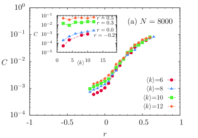
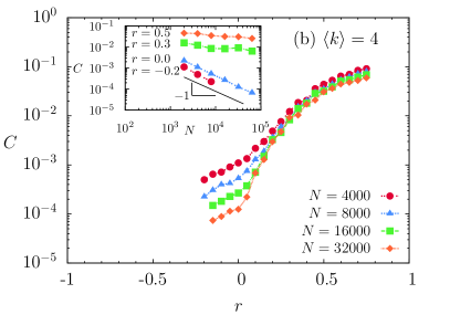
Figure 3: Clustering coefficient $C$ as a function of $r$, as in Fig. 1 but for power-law networks with $\gamma=4.0$: (a) $N=8000$ and different values of $\langle k\rangle$. In the assortative region, $C$ reaches larger values than in the Poisson class. (b) $\langle k\rangle=4$ and different number of nodes $N$. Note that for assortative networks a finite degree of clustering seems to persist for large networks. Standard errors reach 50% for the lowest values of $C$. In the inset, missing values are due to the limitation in attaining the prescribed values of $r$.

The outcomes for the power-law class with $\gamma=4.0$ are displayed in Fig. 3. Standard errors are larger in the power-law case, likely due to the variability in the tails of the distribution of links from sample to sample. Outcomes for the other two values of $\gamma$ studied (3.5 and 4.5) display features similar to those of the case $\gamma=4.0$ used as illustrative example, despite the third moment becoming divergent at $\gamma=4.0$. Two regimes are also observed, with the crossover now closer to $r=0$, but some qualitative differences appear in comparison to the Poisson case. $C$ rapidly increases with $r$, attaining, for assortative networks, larger values than in the Poisson class. These large values are due to the inclusion of highly connected nodes, absent in the Poisson networks, that for large $r_{\star}$ tend to gain links among them, contributing strongly to $r$ and also to $C$.

With respect to finite size effects, below the crossover the small non-null $C$ is again due only to the finite size of the network. However, in the assortative region (above the crossover), it seems that a finite degree of clustering persists for large networks (see inset of Fig. 3(b)), in contrast to the Poisson case and to the dissassortative region. In fact, notice that, when $N$ increases one order of magnitude, $C$ decreases also one order of magnitude in the dissortative region, while $C$ remains of the same order in the assortative interval. Even if $C$ vanished in the infinite size limit, since the decay is very slow, then an effective clustering would remain in moderate, or even large, size networks. We will discuss the interplay between $C$ and $r$ further in Sec. IV. For the mean local clustering coefficient $\bar{C}$, a qualitatively similar dependence on $r$ is observed, but with smaller values. Moreover, $\bar{C}$ increases linearly with $\langle k\rangle$, in the analyzed range, for any fixed $r$, not only for dissortative networks, and $\bar{C}$ decays with $N$ for any $r$. For$r=0$, $C=\bar{C}=(\langle k^{2}\rangle-\langle k\rangle)^{2}/(N\langle k\rangle^{3})$ dorogovtsev , as expected.

Let us analyze now the influence of $r$ on network characteristic lenghts. The dependency of the measures $1/E$, $L$ and $D$ on $r$ is depicted in Fig. 4, for Poisson and power-law distributed networks, with $N=8000$ and $<k>\simeq 4$. $1/E$ and $L$ have close values, systematically shifted. In first approximation both types of network yield similar values of $1/E$ (hence also $L$), given $N$ and $\langle k\rangle$. However, the diameter $D$ is more dependent on the type of network. It is larger and is more strongly affected by $r$ in the homogeneous Poisson case.

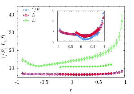
Figure 4: Distance measures $1/E$, $L$ and diameter $D$, as a function of $r$ for Poisson (open symbols) and $\gamma=4.0$ power-law (filled symbols) networks. In all cases $N=8000$ and $\langle k\rangle=4.00\pm 0.04$. The inset is a zoom of the main plot. At first sight, the two types of network display similar values of $1/E$ and $L$, for a given $N$ and $\langle k\rangle$. The diameter is more sensitive to the type of network and is more affected by $r$ in the Poisson case.

Plots of $1/E$ vs $r$ for different values of $N$ and $\langle k\rangle$ are shown in Figs. 5 and 6 for Poisson and power-law networks respectively. In both cases, the networks display the small-world property WS (even smaller in the power-law case) with a slow (logarithmic) increase with $N$ and a smooth decrease with $\langle k\rangle$ (see insets of Figs. 5 and 6).

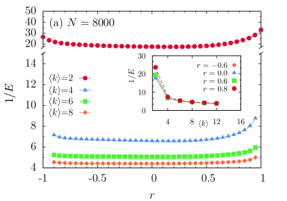
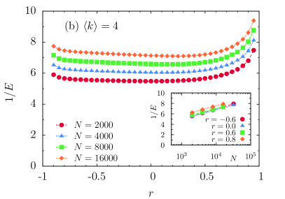
Figure 5: Mean distance $1/E$ as a function of $r$ for Poisson networks: (a) $N=8000$ and different values of $\langle k\rangle$ indicated on the figure. The networks exhibit the small-world property. (b) $\langle k\rangle=4.00\pm 0.04$ and different number of nodes $N$ indicated on the figure. The effects of $r$ on the mean path are significant only for small $\langle k\rangle$ because of the fragmentation of the network.

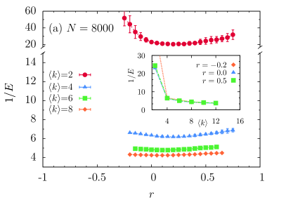
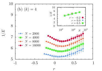
Figure 6: Mean distance $1/E$ as a function of $r$ as in Fig. 5 but for power-law network with $\gamma=4.0$. In this case, paths are shorter than in the Poisson nets.

In the Poisson case, the mean path does not depend on $r$ significantly when $\langle k\rangle$ is not too small ($\geq 6$), as indicated by the relatively flat plots in Fig. 5(a). Only for small $\langle k\rangle$ there are important effects for assortative correlations. For instance, for $\langle k\rangle\simeq 4$ (Fig. 5(b)), $1/E$ increases in about two units from $r\simeq 0$ to $r\simeq 1$, for all the analyzed sizes. This effect is still larger for $\langle k\rangle=2$ where $L$ increases by a factor about two in the same interval of $r$, as shown in Fig. 5(a) for $N=8000$.

In order to further interpret these results, we investigated the cluster structure of the resulting rewired networks. We measured the size of the largest cluster (let us call it $N_{1}$), the number $n$ of clusters, and the average size $S$ of the clusters different from the largest one. The plots are presented in Fig. 7 for $\langle k\rangle=2$ and 4. For $\langle k\rangle=4$, the relative size of the largest cluster (circles) is about 0.98 for most of the range of $r$, notice however that it slightly decays towards $|r|=1$ (which is more evident for $\langle k\rangle=2$). As $\langle k\rangle$ increases, the number of fragments rapidly decays and the average size $S$ (triangles) tends to unit, meaning that only single nodes are disconnected (recall also that $P(0)={\rm e}^{-\langle k\rangle}$). Therefore the increase of the mean distance towards $|r|=1$, observed for low $\langle k\rangle$ in Fig. 5, may simply reflect the fragmentation of the network. Clearly, for high values of the assortativity, the network tends to fragment into groups of vertices that have the same degree. Moreover, for values of $\langle k\rangle$ approximately larger than 1, the percolation analysis performed by Noh on Poisson networks noh shows that the size of the largest cluster is smaller for assortative networks than for dissortative and neutral ones. Meanwhile, as $\langle k\rangle$ increases, the fraction of vertices that do not belong to the largest cluster becomes negligible, although more slowly the more assortative the network. Therefore, in such large $\langle k\rangle$ limit, the mean distance remains invariant under changes of $r$. Hence, transport processes modeled in these networks may suffer important impact when $r$ is large and $\langle k\rangle$ small. The longer the typical separation between nodes, the slower the propagation.

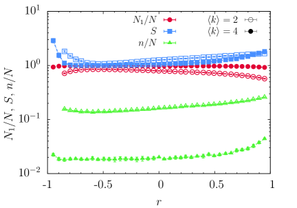
Figure 7: Clusters analysis. Plots of $N_{1}/N$ (where $N_{1}$ is the size of the largest cluster) [circles], average size of finite size clusters, $S$ [squares], and number of clusters, $n$ [triangles], as a function of $r$ for Poisson networks with $\langle k\rangle=2$ (open symbols) and 4 (filled symbols). The fragmentation of the network observed for high values of the assortativity reflects the grouping of vertices with the same degree. The figure shows outcomes for $N=8000$. Outcomes for sizes $N=4000$, 8000 and 16000 all collapse into single curves (not shown).

In power-law networks, for fixed $N$ and $\langle k\rangle>2$, there is an interval of $r$ where paths are shorter than in the Poisson nets (Fig. 4), and still shorter as $\gamma$ decreases (not shown). Moreover $1/E$ becomes more sensitive to the coefficient $r$ (smile shape), in the region where plots are flat for Poisson networks. Notice also that minimal mean paths occur for slightly assortative correlations ($r\gtrsim 0$), slowly increasing with $N$ (Fig. 6(b)). The analysis of clusters for $\gamma=4.0$, shows that for $\langle k\rangle\geq 4$ there is a single cluster of size $N$, for all $r$. Only for $\langle k\rangle=2.0$ we observed fragmentation with $N_{1}/N\simeq 0.7-0.8$, $n/N\simeq 0.06$, $S\simeq 4$ for all $N>2000$ (plots not shown).

For the mean path $L$, we observed qualitatively similar outcomes although shifted to slightly higher values, as illustrated in Fig. 4.

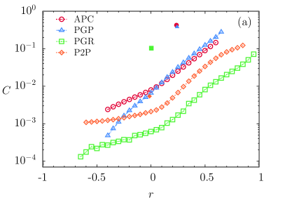
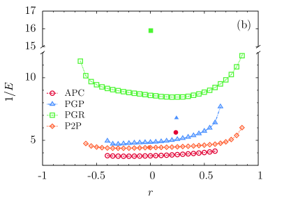
Figure 8: $C$ and $1/E$ vs $r$, for real networks. Original values, before rewiring, are also indicated (filled symbols). PGP (Pretty Good Privacy encrypted communication network) PGP : $N=10680$, $\langle k\rangle\simeq 4.55$; P2P (Gnutella peer-to-peer network) P2P : $N=10876$, $\langle k\rangle\simeq 7.35$; PGR (power grid) PGR , $N=4941$, $\langle k\rangle\simeq 2.67$; APC (astrophysics collaboration) APC : $N=16706$, $\langle k\rangle\simeq 14.5$. Besides the different details of real degree sequences, we can interpret the main features of these nets in terms of those observed for the Poisson and power-law classes.

We also applied the rewiring procedure described in Sec. II to real degree sequences. Networks were symmetrized and edge weights were ignored. In Fig. 8 we depict the behavior of $C$ and $1/E$ vs $r$, for the PGP (encrypted communication network using Pretty Good Privacy encryption algorithm) largest component PGP , P2P (Gnutella peer-to-peer network) P2P , PGR (electrical power grid of the western United States), example of small-world network PGR and APC (astrophysics collaboration network) APC . First notice that in all cases the clustering $C$ is much larger in real networks than in the randomized ($r$-ensemble) ones, as already observed for other examples in Ref. foster . The mean distance is also typically larger in the real networks. An exception is P2P network, characterized by a value of $1/E$ typical of the $r$-ensemble. Rewired real networks display some of the typical behaviors observed for the artificial cases. Let us make some remarks arising from comparisons. (i) PGR (power grid) displays plots of $C$ vs $r$ and $1/E$ vs $r$ that are in good accord with those observed for similar parameters $\langle k\rangle$ and $N$ of the Poisson case. In fact its degree distribution decays exponentially. (ii) P2P presents power-law decay of the degree distributions, for $k>10$, with exponent close to $\gamma=4$. Both plots of P2P are in agreement with those obtained for the $\gamma=4$ class with similar values of $N$ and $\langle k\rangle$, despite the distributions only share in common the power-law tail. (iii) PGP (of size similar to P2P) has a degree distribution that decays with exponent $\gamma<3$ for $k<50$ and $\gamma\simeq 4$ beyond PGP . The plot for $1/E$ vs $r$ presents larger values of $1/E$ than P2P consistent with its $\langle k\rangle$. However, the plot $C$ vs $r$ of PGP deviates from the standard behavior, presenting larger values of $C$ that increase with $r$ in a single regime. The interval of allowed values of $r$ is sensitive also to features other than the tails. These deviations can be attributed to different initial power law regimes. (iv) Finally, APC has a power-law decay with exponent $\gamma\simeq 1$ and exponential cut-off for $k>50$ APC . The low and constant plot of $1/E$ vs $r$ is expected for a network with large $\langle k\rangle$, almost independently of the class of degree distribution. The large values of $C$ are also consistent with heterogeneous distributions with large $\langle k\rangle$.

Then, despite the different details of real degree distributions, the main observed features can be interpreted in terms of the analyzed classes with corresponding values of parameters $\langle k\rangle$ and $N$.

IV Discussion and final remarks

For all classes of networks considered, $C$ increases with $r$ in the whole allowed range of $r$. This behavior has already been observed in Ref. foster , where only positive values of $r$ were analyzed and also in Ref. serrano2 although different definitions of clustering and correlation were used. However, we observed that, in the $r$-ensemble, a non-vanishing clustering coefficient $C$ is typically due to finite size effects, such that, in the large size limit, network transitivity vanishes as $1/N$. In contrast, for power-law networks characterized by $r$ above a threshold, a significantly non-null transitivity arises, apparently persisting for large $N$.

In any case, since rewiring in the $r$-ensemble turns $C$ typically small, transitivity does not seem to contribute for attaining the prescribed value of $r$. To identify the factors that contribute to $r$, it is useful to rewrite Eq. (1). Recalling that $\langle k^{n}\rangle_{e}=\langle k^{n+1}\rangle/\langle k\rangle$ mendes , where $\langle\cdots\rangle$ (without subindex) means computed over the degree distribution $P(k)$, then Eq. (1) becomes

$$r=\frac{\langle k\rangle^{2}\langle kk^{\prime}\rangle_{e}-\langle k^{2}\rangle^{2}}{\langle k\rangle\langle k^{3}\rangle-\langle k^{2}\rangle^{2}}\,.$$ (8)

Following the decomposition made by Estrada estrada , notice that the quantity $\tilde{P}_{3}\equiv\sum_{(k,k^{\prime})}(k-1)(k^{\prime}-1)$, where the sum is performed over all the different pairs of neighboring vertices, is the number of paths of length three, then $\tilde{P}_{3}=3n_{\triangle}+P_{3}$, where $P_{3}$ is the number of nontriangular paths of length three (involving four vertices). As done in Eq. (5) for $3n_{\triangle}$, let us scale also $P_{3}$ by the number of wedges (paths of length two) $P_{2}=\frac{1}{2}\sum_{i}k_{i}(k_{i}-1)$, defining $B=P_{3}/P_{2}$ (scaled branching) estrada . Then Eq. (8) can be written as

$$r=\frac{\langle k\rangle(\langle k^{2}\rangle-\langle k\rangle)\left(B+1-\frac{\langle k^{2}\rangle}{\langle k\rangle}+C\right)}{\langle k\rangle\langle k^{3}\rangle-\langle k^{2}\rangle^{2}}\,.$$ (9)

Expression (9) is determined by the three first raw moments of $P(k)$, and also by $B$ and $C$ that are the quantities embodying the information on the linear degree-degree correlations.

For the Poisson distributed networks, by taking into account the analytical expressions for the moments of $P(k)$, it is straightforward to see that

$$r=B-\langle k\rangle+C\,.$$ (10)

Clearly, dissassortative correlations are favored by vanishing $C$. Only for positive $r$ the growth of $C$ is convenient, but $B-\langle k\rangle$ can vary in a wider interval than $C$ (twice wider in this case). The existence of two regimes in the increase of $C(r)$, observed in Fig. 1, is consistent with this picture. In other words, Eq. (10) indicates that, in the rewiring process of a Poisson network to attain $r_{\star}$, as soon as $P(k)$ is conserved and $C$ remains very small, then $r$ is ruled predominantly by $B$.

For the power-law distributed networks, some qualitatively similar effects occur, as far as the relation of $r$ with $B$ and $C$ is always linear and $C$ is constrained to a narrower interval than $B$. The formation of triangles also in this case contributes only for assortative values of $r$ (above the crossover), with values of $C$ larger than in the Poisson case but still small. Then also in this case the increase of the branching must drive rewiring. In contrast to the Poisson case, the other terms in Eq. (9), related to the moments of $P(k)$, might have a crucial influence on $r$ because of the divergence, in the infinite network limit, of the $n$th moments for $\gamma\geq n+1$.

Let us analyze the large $k_{max}$ (hence $N$) limit, setting aside the marginal (logarithmic) cases. Here, we use the result $k_{max}\sim N$. However, if used instead $k_{c}\sim N^{1/(\gamma-1)}$, the conclusions would remain the same. Considering the expressions for the moments (e.g., Eq. (6)), one has, for $3<\gamma<4$: $r\sim[B-{\cal O}(1)]/{\cal O}(N^{4-\gamma})$, while for $2<\gamma<3$: $r\sim[B-{\cal O}(N^{3-\gamma})]/{\cal O}(N)$, meaning ${\cal O}(x^{\alpha})\sim ax^{\alpha}$, with $a>0$. To approach the lower limit $r=-1$, one must have minimal $B$. If it is of order greater than the other terms in the numerator, then one can not have negative $r$, because $B$ is non-negative and it will dominate the numerator. Thus, negative $r$ can arise only if $B$ is of the same or lower order. But in that case $r\to 0$ in the large $N$ limit. This explains why the lower bound $r_{min}$ tends to 0 when $\gamma\leq 4$ (see Fig. 2(b)). Along this line, however, $r_{min}$ is not expected to vanish when $\gamma>4$, but to tend to a small finite value. Similarly, to attain a non-null upper bound of $r$, $B$ needs to grow like the denominator, otherwise, the upper bound will be negative and also vanish when $N\to\infty$, leading to the collapse of the upper bound too. However, this does not necessarily happens if $B$ is driven to grow enough during rewiring, which is what seems to be happen according to Fig. 2(b).

The connection between $r$ and distance measures is not so direct analytically. Numerical results showed that, for networks with localized distribution of links, changing $r$ modifies significantly the mean path length only when correlations are assortative ($r>0.5$) and $\langle k\rangle$ small. These changes could be related to the induced fragmentation, that diminishes by increasing $\langle k\rangle$. Then, the impact of $r$ becomes less important as $\langle k\rangle$ increases. Meanwhile, the influence on the diameter is more dramatic. In power-law networks, the modification of the mean path length by $r$ is a bit more marked even if fragmentation is absent for $\langle k\rangle\geq 4$, while the diameter is not largely affected. In both cases, the modification of characteristic lengths that occur when varying $r$ may affect transport processes and should be taken into account either when interpreting or designing numerical experiments on top of these networks.

References

- [1] A. Vazquez, Phys. Rev. E 74, 056101 (2006).
- [2] M. Small, X. Xu, J. Zhou, J. Zhang, J. Sun, and J. Lu, Phys. Rev. E 77, 066112 (2008); R. Cohen and S. Havlin, Phys. Rev. Lett. 90, 058701 (2003).
- [3] Y. Xue, J. Wang, L. Li, D. He and B. Hu, Phys. Rev. E 81, 037101 (2010).
- [4] Y. Moreno, J. B. Gómez, A. F. Pacheco, Phys. Rev. E 68, 035103(R) (2003).
- [5] L. K. Gallos, C. Song, H. A. Makse, Phys. Rev. Lett. 100, 248701 (2008).
- [6] M. Boguñá, R. Pastor-Satorras, Phys. Rev. E 66, 047104 (2002).
- [7] M. Boguñá, R. Pastor-Satorras, A. Vespignani, Phys. Rev. Lett. 90, 028701 (2003).
- [8] A. Pusch, S. Weber, M. Porto, Phys. Rev. E 77, 017101 (2008).
- [9] J. Menche, A. Valleriani, R. Lipowsky, Phys. Rev. E 81, 046103 (2010).
- [10] M. E. J. Newman, Phys. Rev. E 67, 026126 (2003).
- [11] R. Xulvi-Brunet, I. M. Sokolov, Phys. Rev. E 70, 066102 (2004).
- [12] M. E. J. Newman, Phys. Rev. Lett. 89, 208701 (2002).
- [13] M. A. Serrano, M. Boguñá, R. Pastor-Satorras, A. Vespignani, Correlations in Complex Networks. In Large scale structure and dynamics of complex networks: From Information Technology to Finance and Natural Sciences, G. Caldarelli, A. Vespignani, editors, (World Scientific, Singapore, 2007).
- [14] J. Park, M. E. J. Newman, Phys. Rev. E 70, 66117 (2004).
- [15] D. V. Foster, J. G. Foster, P. Grassberger, M. Paczuski, Phys. Rev. E 84, 066117 (2011).
- [16] J. D. Noh, Phys. Rev. E 76, 026116 (2007).
- [17] E. Estrada, Phys. Rev. E 84, 047101 (2011).
- [18] M. Serrano and M. Boguñá, Phys. Rev. E 74, 056114 (2006).
- [19] S. N. Dorogovtsev, Phys. Rev. E 69, 027104 (2004).
- [20] M. E. J. Newman, PNAS 98 (2), 404 (2001).
- [21] D. J. Watts and S. H. Strogatz, Nature (London) 393, 440 (1998).
- [22] S. Boccaletti, V. Latora, Y. Moreno, M. Chavez, D.-U. Hwang, Phys. Reps. 424, 175 (2006); V. Latora and M. Marchiori, Phys. Rev. Lett. 87, 198701 (2001).
- [23] A. Barrat and M. Weigt, Eur. Physics J. B 13, 547 (2000).
- [24] M. E. J. Newman, S. H. Strogatz and D. J. Watts, Physical Review E 64, 026118 (2001).
- [25] P. Erdős and A. Rényi, Publ. Math. 6, 290 (1959); R. Albert, A. L. Barabási, Rev. Mod. Phys. 74, 47 (2001).
- [26] M. Molloy and B. Reed, Random Structures & Algorithms 6 161 (1995); M. E. J. Newman, Networks: An Introduction (Oxford University Press, Inc., New York, NY, USA, 2010).
- [27] S. M. Ross, Simulation (Academic Press, 2006); M. E. J. Newman, G. T. Barkema, Monte Carlo Methods in Statistical Physics (Oxford University Press, USA, 1999).
- [28] S. N. Dorogovtsev, and J. F. F. Mendes, Adv. Phys. 51, 1079 (2002)
- [29] S. Maslov, K. Sneppen, Science 296, 910 (2002).
- [30] D. Foster, J. Foster, and M. Paczuski, Phys. Rev. E 81, 046115 (2010).
- [31] M. E. J. Newman, Proc. Natl. Acad. Sci. USA 98, 404 (2001); Data at http://www-personal.umich.edu/~mejn/netdata
- [32] J. Park and M. E. J. Newman, Phys. Rev. E 68, 026112 (2003).
- [33] S. N. Dorogovtsev, J. F. F. Mendes and A. N. Samukhin, Phys. Rev. Lett. 85, 4633 (2000).
- [34] M. Boguñá, R. Pastor-Satorras, A. Díaz-Guilera, A. Arenas, Phys. Rev. E 70, 056122 (2004).
- [35] Data can be found at http://snap.stanford.edu/data/p2p-Gnutella04.html
- [36] D. J. Watts, S. H. Strogatz, Nature 393, 440 (1998); data can be found at http://www-personal.umich.edu/~mejn/netdata
- [37] S. N. Dorogovtsev, A. L. Ferreira, A. V. Goltsev, J. F. F. Mendes, Phys. Rev. E 81, 031135 (2010).