Spin polarization and $g$-factor enhancement in graphene nanoribbons in magnetic field

Abstract

We provide a systematic quantitative description of spin polarization in armchair and zigzag graphene nanoribbons in a perpendicular magnetic field. We first address spinless electrons within the Hartree approximation studying the evolution of the magnetoband structure and formation of the compressible strips. We discuss the potential profile and the density distribution near the edges and the difference and similarities between armchair and zigzag edges. Accounting for the Zeeman interaction and describing the spin effects via the Hubbard term we study the spin-resolved subband structure and relate the spin polarization of the system at hand to the formation of the compressible strips for the case of spinless electrons. At high magnetic field the calculated effective $g$-factor varies around a value of $\left\langle g^{\ast}\right\rangle\approx 2.25$ for armchair nanoribbons and $\left\langle g^{\ast}\right\rangle\approx 3$ for zigzag nanoribbons. An important finding is that in zigzag nanoribbons the zero-energy mode remains pinned to the Fermi-energy and becomes fully spin-polarized for all magnetic fields, which, in turn, leads to a strong spin polarization of the electron density near the zigzag edge.

I Introduction

Investigation of effects of electron interaction and spin in graphene at high magnetic field represents one of the frontiers in the graphene research. Even though many aspects of the magnetoconductance of graphene related to the formation of unconventional Landau level spectra and the anomalous Hall effect are well understood theoretically and confirmed experimentallyCastro_Neto_review ; GusyninQHE ; Novoselov2005 ; Zhang , there are still a number of questions awaiting their resolution. One of these questions which is extensively debated in the current literature is the origin of the splitting of the lowest Landau level and the emerging of insulating state at the Dirac point.Zhang2006 ; Jiang ; Checkelsky ; Zhang2009 ; Zhao12 Even though the precise origin of this state is under current debate, it is generally believed that it is related to electron-electron interaction and spin effects. The importance of electron interaction was also outlined for higher Landau levels Jiang . Recently, spin-splitting in graphene and bilayer graphene in high magnetic field was experimentally analyzed by Kurganona et al.Kurganova , who found that $g$-factor in graphene is enhanced, and attributed this to electron-electron interaction effects. The spin-splitting of the states in grapheneFolk and graphene quantum dotsGuttinger was also studied in a parallel magnetic filed.

Motivated by this interest to the electron interacton and spin effects in graphene in the high magnetic field, in the present paper we study the spin polarization and enhancement of the $g$-factor in graphene nanoribbons (GNRs). Note that various aspects of electron and spin interactions in high magnetic have been extensively studied in conventional semiconducting quantum wires defined in two dimensional electron gas (2DEG) Kinaret ; Dempsey ; Tokura ; takis2002 ; Stoof ; Ihnatsenka_wire1 ; Ihnatsenka_wire_comp_strips ; IhnatsenkaCEOQW ; IhnatsenkaMarcus . One of the motivations for such studies is related to advances in semiconductor spintronics utilizing the spin degree of freedom for adding new functionalities to electronic devices.spintronics Some of proposed and investigated devices for spintronics and quantum computation applications operates in the edge state regime,adot ; Giovannetti which obviously requires a detailed knowledge of the structure of the states in a quantum wire or at the edge of the 2DEG. The properties and detailed information about propagating states at the boundaries are also essential for interpretation of experiments in various electron interferometers in the quantum Hall regimeCamino ; IhnatsenkaKirzcenow ; Paradiso . Because graphene represents a very promising system for implementation of many devices and concepts for spintronics and quantum information processing applications utilizing the edge state transport regime a detailed knowledge of the density and potential profiles near the edges as well as spin properties are important for understanding and designing of such devices.

The paper is organized as follows. In Sec. II we present a formulation of the problem, define the Hamiltonian and briefly outline the self-consistent computational scheme. The results and discussion are presented in Sec. II. Section IIA discusses the potential profile and the charge accumulation near the edges in ribbons of different widths and edge terminations. Section IIB is devoted to the case of spinless electrons focussing on the formation of compressible strips and evolution of the magnetoband structure. Finally, based on the results of Sec. IIB, Sec. IIC discusses the spin splitting and the enhancement of the $g$-factor for the case of electrons with spin. The conclusions of the work are presented in Sec. III.

II Model

We consider an infinite GNR of the width $W$, located in an insulating substrate with the relative permittivity $\epsilon_{r}$ and subjected to the perpendicular magnetic field $B$, see inset to Fig. 1(b). A metallic back gate situated at the distance $d$ from the ribbon is used to tune the Fermi energy in order to change an electron concentration in the GNR. The system is modeled by the p-orbital tight-binding Hubbard-type Hamiltonian in the mean-field approximation, $H=H^{\uparrow}+H^{\downarrow},$ which is shown to describe carbon electron systems in good agreement with the first-principles calculationsPalacios ; Yazyev ,

$$H^{\sigma}=-\sum_{\mathbf{r},\Delta}t_{\mathbf{r},\mathbf{r}+\Delta}a_{\mathbf{r}\sigma}^{+}a_{\mathbf{r}+\Delta,\sigma}$$ (1)

$$+\sum_{\mathbf{r}}\left(V_{Z}^{\sigma}+V_{H}(\mathbf{r})+V_{U}^{\sigma^{\prime}}(\mathbf{r})\right)a_{\mathbf{r}\sigma}^{+}a_{\mathbf{r}\sigma}$$

where $\sigma$, $\sigma^{\prime}$ correspond to two opposite spin states $\uparrow$, $\downarrow$; the summation runs over all sites $\mathbf{r=(}x,y\mathbf{)}$ of the graphene lattice, $\Delta$ includes the nearest neighbors only. The magnetic field is included in a standard way via the Pierel’s substitution, $t_{\mathbf{r},\mathbf{r}+\Delta}=t_{0}\exp(i2\pi\phi_{\mathbf{r},\mathbf{r}+\Delta}/\phi_{0})$ where $\phi_{\mathbf{r},\mathbf{r}+\Delta}=\int_{\mathbf{r}}^{\mathbf{r}+\Delta}\mathbf{A}\cdot d\mathbf{l},$ with $\mathbf{A}$ being the vector potential, and $\phi_{0}=h/e$ being the magnetic flux quantum, $t_{0}=2.7$ eV. (In our calculations we use the Landau gauge, $\mathbf{A}=(-By,0)$). The first two terms in Eq. (1) correspond to the non-interacting part of the Hamiltonian, with the first term describing the kinetic energy of the electrons on a graphene lattice. The second term describes the Zeeman energy triggering the spin-splitting in the magnetic field, $V_{Z}^{\sigma}=\pm\frac{1}{2}g\mu_{b}B,$ where $+(-)$ signs correspond to the opposite spin states $\uparrow$ $(\downarrow);$ $g=2$ is the bare $g$-factor of pristine graphene, and the Bohr magneton $\mu_{b}=e\hbar/2m_{e}.$ The two last terms in Eq. (1) describe the electron interaction. The long-range Coulomb interaction between induced charges in the GNR is given by the standard Hartree term,

$$V_{H}(\mathbf{r})=\frac{e^{2}}{4\pi\varepsilon_{0}\varepsilon_{r}}\sum_{\mathbf{r}^{\prime}\neq\mathbf{r}}n_{\mathbf{r}^{\prime}}\left(\frac{1}{|\mathbf{r}-\mathbf{r}^{\prime}|}-\frac{1}{\sqrt{|\mathbf{r}-\mathbf{r}^{\prime}|^{2}+4d^{2}}}\right),$$ (2)

where $n_{\mathbf{r}}=n_{\mathbf{r}\uparrow}+n_{\mathbf{r}\downarrow}$ is the total electron density, and the second term corresponds to a contribution from the mirror charges. The last term in the Hamiltonian (1) corresponds to the Hubbard energy,

$$V_{U}^{\sigma^{\prime}}(\mathbf{r})=U\left(n_{\mathbf{r}}^{\sigma^{\prime}}-\frac{1}{2}\right),$$ (3)

and describes repulsion between electrons of the opposite spins on the same site. The number of excess electron at the site $\mathbf{r}$ reads,

$$n_{\mathbf{r}}^{\sigma}=\int_{-\infty}^{\infty}\rho^{\sigma}(\mathbf{r},E)f_{FD}(E,E_{F})dE-n_{\text{ions}},$$ (4)

where $\rho^{\sigma}(\mathbf{r},E)=-\frac{1}{\pi}\Im[G^{\sigma}(\mathbf{r},\mathbf{r},E)]$ is the energy dependent local density of states (LDOS) at rero temperature; $G^{\sigma}(\mathbf{r},\mathbf{r},E)$ is the Green’s function in the real space representation of an electron of the spin $\sigma$ residing on the site $\mathbf{r}$, $E_{F}=eV_{g}$ is the Fermi energy which value is adjusted by the gate voltage, and $n_{\text{ions}}=1/A_{0}=3.8\times 10^{19}$m^-2 is the positive charge background of ions ($A_{0}=\frac{3\sqrt{3}}{4}a_{0}^{2}$ is the area per one C atom and $a_{0}=0.142$ nm is the C-C distance). Equations (1)-(4) are solved self-consistently using the Green’s function technique in order to calculate the band structure, the charge density and the potential distribution.Xu ; Shylau10 ; Shylau11 For a given potential distribution we compute the conductance using the Landauer formula

$$\mathcal{G}^{\sigma}(E_{F})=\frac{e^{2}}{h}\int T^{\sigma}(E)\left[-\frac{\partial f_{FD}(E-E_{F})}{\partial E}\right]dE,$$ (5)

where $T^{\sigma}(E)$ is the total transmission coefficient for electrons with spin $\sigma$, and $f_{FD}$ is the Fermi-Dirac distribution.

III Results and discussion

III.1 Potential profile and the charge accumulation near the edges in ribbons of different widths and edge terminations.

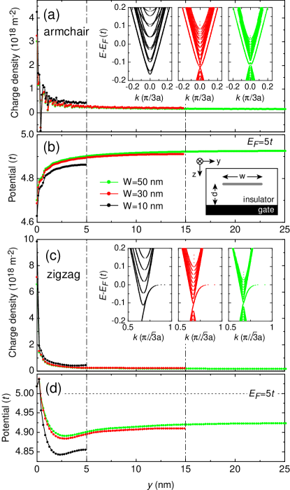
Figure 1: (Color online). (a),(c) The self-consistent charge densities and (b),(d) potentials for the armchair and zigzag ribbons of widths $W$=10,30 and 50 nm calculated in the Hartree approximation at zero magnetic field. Only half of the ribbon is shown. The insets in (a),(c) show the dispersion relation for nanoribbons of different widths $W$=10, 30 and 50 nm from the left to the right for several lowest subbands.The inset in (b) shows a schematically geometry of the device; $d=30$ nm. $E_{F}$=5 $t$. $t=2.7$ eV. $a=0.142$ nm.

In the present study we aim at the description of spin polarization in realistically wide GNRs. In current experimentsMolitor ; Oostinga ; Poumirol ; Ribeiro the widths of nanoribbons are $W\sim 100$ nm and the magnetic field reaches $B\lesssim 60$ T, corresponding to the ratio $W/l_{B}\approx 10$, with $l_{B}=\sqrt{\hbar/eB}$ being the magnetic length. At the same time, because of computational limitations, it is difficult to treat ribbons of widths exceeding 50 nm. Therefore in our calculations we re-scale the system using ribbons of smaller width $W\sim 30$ nm subjected to higher fields (up to $B\sim 350$ T) in order to keep the ratio $W/l_{B}\approx 10$ in accordance with typical experiments.Molitor ; Oostinga ; Poumirol ; Ribeiro In very narrow ribbons the quantum confinement effects can dominate ribbon’s electronic properties. Thus, a concern might arise whether the obtained results remain valid for realistically wide ribbons. In the present section we investigate how nanoribbon’s electronic properties such as the density distribution and the potential profile in the vicinity of the edge change with the increase of the ribbon’s width, and find that the width of $W\approx 30$ nm is already sufficient to capture all essential features of a wide ribbon or even a semi-infinite graphene sheet.

In our study we consider both types of edges, armchair and zigzag. We will demonstrate in the subsequent sections that main features in the spin polarization of the electron density and the enhancement of the $g$-factor are rather similar for both types of edges. There is however an important difference between them which can be traced to the presence of the zero-energy mode (ZEM) residing at the edge of the zigzag GNRs.Wakabayashi In the present section we will demonstrate that the ZEM leads to a different features in the potential and charge density profiles near the edges for the cases of armchair and zigzag ribbons.

Figure 1 shows the self-consistent charge density distributions and potential profiles for the armchair and zigzag nanoribbons of various widths $W$=10, 30, 50 nm. In all calculation the distance between the GNR and the gate is $d=30$ nm. The calculations are performed in the Hartree approximation for spinless electrons at zero field (i.e. $V_{U}^{\sigma}$ and $V_{Z}^{\sigma}$ are set to $0$ in the Hamiltonian (1)). It is noteworthy that the electron density distribution obtained from the electrostatics (i.e. due to the Hartree potential $V_{H}(\mathbf{r}),$ Eq. (2)) is not altered significantly by magnetic field Chklovskii . The charge densities and potentials stay qualitatively the same as the nanoribbon width increases and exhibit practically no difference for 30- and 50-nm wide nanoribbons. We thus conclude that the transverse confinement does not change substantially for nanoribbons wider than $\sim 30$ nm, and the width $W=30$ nm is sufficient to describe realistically wide ribbons or even an edge of a graphene sheet.

Let us now focus on a difference in the potential profiles and the electron density distributions in a vicinity of a ribbon edge for armchair and zigzag ribbons. Both ribbons show strong electron accumulation near the edges but this accumulation is stronger in the zigzag GNRs. The corresponding potential profiles for armchair and zigzag ribbons have different shapes near the edges. For the armchair ribbon, the potential has a triangular shape, see Fig. 1(b). This was predicted and explored previously.Silvestrov08 ; Shylau09 The triangular shape of the potential is related to the hard-wall confinement. It is noteworthy that a similar triangular shape of a potential is exhibited by cleaved-edge overgrown quantum wires where electrons also experience a hard-wall confinement. Grayson ; IhnatsenkaCEOQW .

The potential profile for the case of zigzag ribbon exhibits somehow different features. As in the case of the armchair GNRs, it gradually decreases towards the boundaries to form a well in the vicinity of the edges. However, in the close proximity to the edges, it raises up and crosses the Fermi energy, see Fig. 1(d). We relate this feature to the zero-energy mode (ZEM) that traps charges. The zero-energy mode is manifested as disperseless energy level pinned to $E_{F}$ in the ranges $k\in\frac{\pi}{\sqrt{3}a}\left[\frac{2}{3},1\right]$ and $k\in-\frac{\pi}{\sqrt{3}a}\left[\frac{2}{3},1\right]$. It is these trapped charges that raise the potential at the edges. They effectively repulse excess charges induced in the ribbon by the gate and prevent the triangular well to form near the boundary. Therefore, the difference in the charge accumulation and potential profiles in the armchair and zigzag ribbons occurs due to topological property of the zigzag edge termination supporting the zero-energy mode. It is important to stress that this difference persists into the high-field regime and can not be addressed by semi-classical approaches like in Ref. Silvestrov08, .

III.2 LDOS, magnetobandstructure and formation of compressible strips for spinless electrons

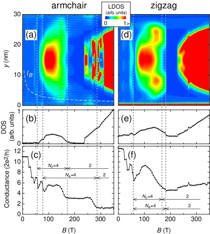
Figure 2: (Color online). (a),(d) The LDOS and (b),(e)the DOS at the Fermi energy, and (c),(f) the two-terminal conductance calculated in the Hartree approximation for the armchair and zigzag ribbons (left and right panels respectively). The LDOS is shown for one graphene sublattice, say A; The LDOS for the sublattice B is symmetric with respect to the ribbon’s axis. The regions with higher LDOS point to higher probability to find an electron there and correspond to positions of the compressible strip. $N_{c}$ and $N_{e}$ in (c) and (f) mark the number of occupied electron subbands in the center and near the edge of the ribbon respectively. The width of ribbons is $W=30$ nm corresponding to 242 and 141 carbons in the cross section of armchair and zigzag ribbons, respectively. $E_{F}$=5 $t$. The temperature $T=10$ K.

Spin polarization in conventional quantum wires is related to the formation of compressible stripsChklovskii in the case of interacting spinless electrons.Ihnatsenka_wire_comp_strips ; IhnatsenkaCEOQW ; IhnatsenkaMarcus In this section we therefore outline the electronic and transport properties of armchair and zigzag nanoribbons in the Hartree approximation for spinless electrons (i.e. disregarding the Hubbard and the Zeeman interactions, $V_{Z}=$ $V_{U}=0$, in the Hamiltonian Eq. (1)) focussing on the formation of the compressible strips.

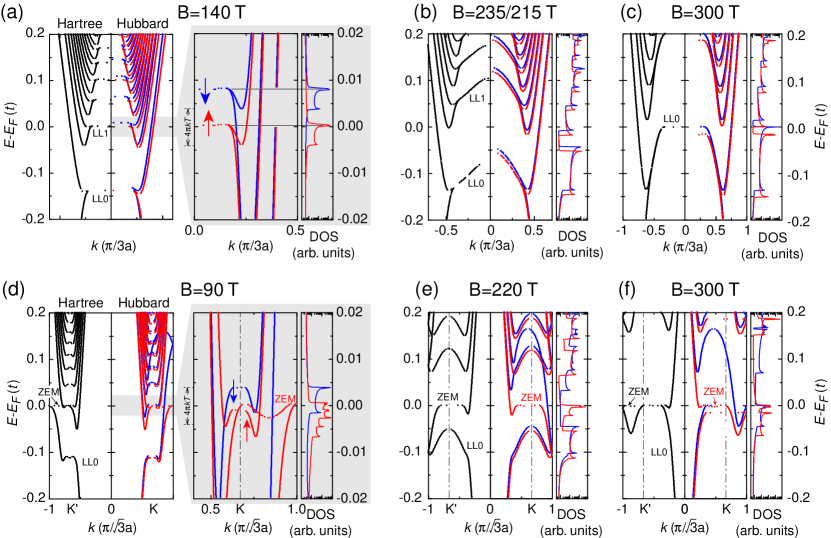
Figure 3: (Color online). The dispersion relation for (a)-(c) the armchair and (d)-(f) the zigzag ribbons. Left and right panels in every plot correspond respectively to the Hartree and Hubbard approximations. Because of the symmetry, only a half of the band diagrams is shown. The red and blue dotted lines show respectively spin-up and spin-down components. Vertical dot-dashed lines in (d)-(f) mark $K$ and $K^{\prime}$ points of the first Brillouin zone of graphene in the zigzag ribbon. In armchair ribbon, $K$ and $K^{\prime}$ points coincide at $k=0$. In (d)-(f), ”ZEM” marks the zero-energy mode that stays pinned to the Fermi energy.

Figures 2(a) (b) show the local density of states (LDOS), $LDOS(y)=-\int\rho(y,E)\frac{\partial f_{FD}(E-E_{F})}{\partial E}dE$, and the total density of states (DOS), $DOS=\sum_{y}LDOS(y)$, at the Fermi energy as a function of the magnetic field for the armchair and zigzag ribbons. (Note that LDOS is shown for one sublattice only.) It is noteworthy that the DOS can be accessible via magneto-capacitance or magnetoresistance measurements similarly to conventional semiconductor structures defined in 2DEGWeiss89 ; Berggren98 . The structure of the LDOS and DOS can be understood from an analysis of the magnetosubband structure. We outline below the main features of the subband structure for the armchair and zigzag ribbons focussing on the differences and similarities between them as well as on formation of the compressible strips in the ribbons. (Note that evolution of the band structure for the case of the armchair GNRs was discussed by Shylau et al.Shylau10 ).

Left panels of Figs. 3 (a)-(c) show the band structure of armchair graphene nanoribbons for spinless Hartree electrons for three representative magnetic fields. Flat regions in the band diagrams correspond to the Landau levels in bulk graphene, and dispersiveness states close to the GNRs boundaries represent edge states corresponding to classical skipping orbits. Figure 3 (a) shows the band diagram for a magnetic field $B=140$ T when the two lowest Landau levels, LL0 and LL1, are filled. The first Landau level LL1 is pinned to the Fermi energy thus forming a compressible strip in the center of the GNR. The strip is called compressible when the electron density can be easily redistributed in order to effectively screen the external potential. We define a compressible strip as a region where the dispersion lies within the energy window $|E-E_{F}|\lesssim 2\pi k_{B}T$ Ando ; Ihnatsenka_wire1 ; Ihnatsenka_wire_comp_strips ; Shylau10 because in this energy window the states are partially filled i.e., $0<f_{FD}<1$ and thus the electron density can be easily changed.

Because a graphene ribbon has abrupt edges the self-consistent potential forms the triangular wells near edges as discussed in the previous section. As a result the center of the ribbon and its edges depopulate in magnetic field differently. Namely, as the magnetic field increases, the subbands first depopulate in the center and then near the edges. For example, the second subband (i.e. LL1) is pinned to the Fermi level in the ribbon center in the interval $B\approx 60-170$ T. Within this interval it forms the compressible strip which is manifested itself as the enhanced LDOS and DOS in Figs. 2(a) and (b). However, the LL1 stays populated near the edges in a wider magnetic field range, $B\approx 80-290$ T . In the field interval $B\approx 170-230$ T the LL1 is depopulated in the center (see Fig. 3 (b)). As a result the LDOS and DOS are practically zero, see Figs. 2 (a),(b). When the magnetic field increases to $B\approx 230$ T, the lowest Landau level, LL0, is pushed up in energy and gets pinned to the Fermi energy. This again leads to a formation of the compressible strip in the middle of the wire (see Fig. 3 (b)) and to the enhancement of the LDOS and DOS at the Fermi energy as seen in Figs. 2 (a),(b). At this $B$, two different LLs are at $E_{F}$ and contribute to electron transport: LL0 in the center and LL1 near the edges.

The graphene ribbons with the zigzag edge termination exhibits features of the magnetosubband structure similar to those for the armchair terminated ribbons. This is illustrated in Figs. 3 (d)-(f) which show the band structure of the zigzag GNRs for three representative magnetic fields, $B=90$ T, 220 T and 300 T. As for the armchair GNRs, these fields correspond respectively to the cases when the LL1 is pinned to $E_{F}$ in the middle of the GNR (Fig. 3 (d)), LL1 is depopulated in the middle of the GNR (Fig. 3 (e)), and LL0 is pinned to $E_{F}$ in the middle of the GNR (Fig. 3 (f)). However, there are several striking differences between the zigzag and armchair ribbons manifested in their LDOS, DOS and the subband structure. First, strong electron accumulation and formation of the compressible strip takes place near the very ribbon’s boundaries over all the range of magnetic fields studied, see enhanced LDOS at $y\sim 0$ in Fig. 2(d). Because of this the total DOS in the zigzag GNR never drops to zero over all the range of magnetic fields, see Fig 2(e). (Note that Fig. 2(d) shows the LDOS for the sublattice A which is enhanced at the one edge of the ribbon. The sublattice B has the enhanced LDOS near the opposite edge of the ribbon).

Inspection of the magnetoband structure reveals that these features are caused by the ZEM in the zigzag GNR discussed in the previous section. This mode (marked by ”ZEM” in Figs. 3 (d)-(f)) always stays pinned to the Fermi energy because of the high density of states for electrons that this mode accommodates. It is important to stress that the pinning of this mode to $E=E_{F}$ is the result of the electron-electron interaction, and the pinning effect is apparently absent in the one-electron description where this mode the is always situated at $E=0$.Wakabayashi

Figures 2(c),(f) show evolution of the two-terminal conductance as the magnetic field increases for the armchair and zigzag ribbons. In contrast to the conventional semiconductor quantum wires and quantum point contacts exhibiting a step-like conductanceQPC , the conductance of GNRs reveals non-monotonic decrease with bumps coexisting with quantized plateau regions of multiples $\frac{2e^{2}}{h}$. Note that $\mathcal{G}$ changes by two conductance quantum between plateaus due to valley degeneracy of graphene. The origin of the bumps in the conductance was discussed by Shylau et al. Shylau10 and was related to the interaction-induced modifications of the band structure leading to the formation of compressible strips in the middle of GNRs.

III.3 Spin splitting and the enhancement of the $g$-factor

Let us now turn to the case of electrons with spin and analyze how the Hubbard and the Zeeman interactions modify the magnetosubband structure of graphene nanoribbons leading to the spin polarization and enhancement of the $g$-factor. For the Hubbard constant we choose $U=t$ which corresponds to the estimation of Refs. Yazyev ; Jung . Note that the recent workWehlingKatsnelson2011 predicts a somehow larger value, $U\approx 3t.$ While the utilization of larger value of $U$ leads to some quantitative differences with the results presented below, they remain qualitatively the same and the conclusions are not affected. We also stress that while the discussion below is focused on the case of high magnetic field when the two lowest Landau levels, LL1 and LL0, are occupied, the similar conclusion remain valid for lower fields as well.

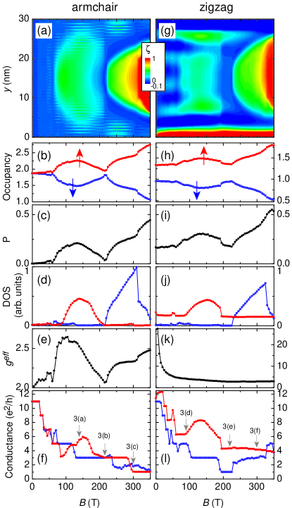
Figure 4: (a),(g) The local spin polarization of the charge density, (b),(h) the unit cell occupancy, (c), (i) the spin polarization $P$, (d),(j) the DOS, (e), (k) the effective $g$-factor, and (f),(l) the conductance as a function of magnetic field calculated in the Hubbard approximation for the armchair (a)-(f) and zigzag (g)-(l) ribbons. The red lines with filled dots show spin-up component and blue line with open squares is for spin-down. Arrows in (f) and (l) mark magnetic fields for the band structures shown in Fig. 3.

Let us start with the case of the armchair ribbons. Figures 4 (a)-(c) show the local spin polarization of the charge density, $\zeta(y)=\frac{n^{\uparrow}(y)-n^{\downarrow}(y)}{n^{\uparrow}(y)+n^{\downarrow}(y)},$ spin-resolved densities and the total spin polarization, $P=\frac{n^{\uparrow}-n^{\downarrow}}{n^{\uparrow}+n^{\downarrow}},$ ($n^{\sigma}=\sum_{y}n^{\sigma}(y)$) as a function of magnetic field. The features in $\zeta(y)$ show a striking similarity with the features of the LDOS, and the behavior of the $P$ follows that one of the DOS calculated in the Hartree approximation (c. f. Fig. 2 (a),(b)). This similarity is not coincidental. The regions with the enhanced LDOS correspond to compressible strips, and it is the compressible strips where the spin splitting of subbands takes place. Indeed, in the compressible region the subbands are only partially filled because $f_{FD}<1$ there, and, therefore, the population of the spin-up and spin-down subbands can be easily changed. This population difference triggered by Zeeman splitting is enhanced by the Hubbard interaction leading to different effective potentials for spin-up and spin-down electrons and eventually to the subband spin splitting.

For a more detailed analysis let us follow an evolution of the band structure in Fig. 3(a)-(c). The right panel of Fig. 3 (a) shows a spin-resolved magnetoband structure corresponding to the case when LL1 forms a compressible strip in the middle of the ribbon for the case of spinless electrons (c.f. the left panel of the figure). The Hubbard interaction pushes up the spin-down subbands above the window $|E-E_{F}|\approx 2k_{B}T$ such that it becomes depopulated, and the compressible strip in the middle is occupied by spin-up electrons only. As a result, the DOS at $E_{F}$ of the spin-up electrons is enhanced, while that one of the spin-down electrons is zero, see Fig. 4 (d). All these lead to the difference in the electron densities $n^{\uparrow}$ and $n^{\downarrow}$ and the spin polarization in the ribbon as shown in Figs. 4 (b) and (c). When the magnetic field increases such that the LL1 is pushed above the $E_{F},$ the compressible strip in the middle disappears, the DOS at $E_{F}$ for both spin species becomes equal to zero and the spin polarization vanishes. This is illustrated in the band diagram shown in Fig. 3 (b) corresponding to the case when $E_{F}$ is situated between LL0 and LL1. With further increase of the magnetic field the LL0 is pushed up to $E_{F}.$ As this subband is pushed from below, in this case it is the higher energy spin-down state that gets pinned to $E_{F}$ forming a compressible strips, whereas the spin-up subband in the middle of the ribbon remains below the $|E-E_{F}|\approx 2k_{B}T.$ As a result, for this case the DOS at $E_{F}$ for the spin-down electrons is larger than that for the spin-up electrons, Fig. 4(d). Note that despite of this, $n^{\uparrow}>n^{\downarrow}$ (see Fig. 4 (b)) because the spin-up subband is fully occupied, whereas the spin-down subband is occupied only partially.

Figure 4(e) shows the effective $g^{\ast}$-factor for the armchair ribbon defined according to $g^{\ast}=\langle V^{\uparrow}-V^{\downarrow}\rangle/\mu_{B}B$, where the averaging is done over all carbon atoms. Because the electron density is related to the potential, the features in the $g^{\ast}$-factor resemble those of the polarization $P,$ showing the behavior reflecting successive population and depopulation of the spin-up and spin-down subbands.

In high magnetic field, $B\gtrsim 50$ T, (corresponding to population of LL1 and LL0) the effective $g$-factor varies between $2.1\lesssim g^{\ast}\leq 2.7$ with the average value $\left\langle g^{\ast}\right\rangle\approx 2.25$, which represents a rather modest enhancement in comparison to the case of noninteracting electrons in pristine graphene with $g=2$. Note that in the bulk graphene the effective $g^{\ast}$-factor was reported to be $g^{\ast}\approx 2.7.$ Kurganova

It is worth mentioning that the main features of the spin polarization and the subband evolution in magnetic field resemble those in the cleaved-edge overgrown quantum wires (CEOQW) IhnatsenkaCEOQW . This is because in both cases the potential corresponds to the hard-wall confinement. The difference is that in CEOQW, as well as in conventional GaAs split-gate wiresIhnatsenka_wire1 , the polarization and thus the effective $g^{\ast}$-factor are enhanced by a factor of $\sim 10$ in comparison to the Zeeman splitting, whereas in the armchair ribbons this enhancement it is just $\sim$ 0.22. This can be explained by fact that the bare $g$-factor in armchair GNRs is much larger that that one in GaAs ( $g_{\text{GaAs}}/g_{\text{graphene}}\approx 0.022$), such that Zeeman interaction in graphene remains dominant in comparison to the exchange one.

One more important difference of the graphene ribbons from the conventional GaAs quantum wires is in the character of spin polarized edge states in the vicinity of the boundaries. In the conventional quantum wires the edge state of opposite spins are spatially separated.Ihnatsenka_wire_comp_strips This is ultimately related to the formation of the compressible strips near the boundaries of the split-gate wire because of the soft confinement due to the gates.Ihnatsenka_wire_comp_strips In GNR due to the hard-wall confinement the compressible strips do not form near the boundaries, and hence the spatial separation of the edge states of opposite spins does not occur. It is worth mentioning that in this respect the GNRs are also similar to CEOQW.IhnatsenkaCEOQW

Let us now turn to the case of zigzag nanoribbons. The main features of the spin polarization and the subband evolution are rather similar to the armchair ones. There is however one important difference related to the presence of the zero-energy mode residing at the zigzag edges. In contrast to other modes exhibiting successive population and depopulation of the Landau levels in the middle of the ribbon, this mode always stays pinned to $E_{F}$ thus forming a compressible strip with the enhanced density of states at the edges for all magnetic fields . The Hubbard interaction leads to a complete spin polarization such that electrons in this mode are always in the spin-up state. This is seen in the spatially-resolved polarization shown in Fig. 4(g). Because of this the total spin-up density is significantly larger than the spin-down one for all magnetic fields, and the DOS for spin-up electrons never drops to zero. This is in contrast to the case of armchair GNRs where electron densities for opposite spin species can be equal when the Fermi energy lies between two consecutive Landau levels, and where both DOS for spin-ups and spin-downs can drop to zero (c.f. Figs. (d) with (j)). Because of the strong polarization near zigzag edges, the effective $g^{\ast}$-factor is strongly enhanced at low field (when the Zeeman spliting is small), and at higher fields it decreases to values $g^{\ast}\approx 3$ comparable to those in the armchair GNRs, see Fig. 4 (k).

Figures 4(f),(l) show evolution of the two-terminal conductance as the magnetic field increases for the armchair and zigzag ribbons. The conductance is apparently spin polarized with $\mathcal{G}^{\uparrow}\neq$ $\mathcal{G}^{\downarrow}$. This reflects the fact that at a given magnetic field the number of propagating states at $E_{F}$ accommodating spin-up and spin-down electrons are different. As in the case of spinless electrons, the spin-resolved conductance also exhibits a bump-like structure which origin is the same as for the case of spinless electrons. Note that because of the presence of a spin-polarized zero-energy mode, the spin-up conductance is larger than spin-down one for most fields. Finally we stress that Figs. 4(f),(l) show the conductances of ideal GNRs without defects. The defects scattering will modify GNRs conductance, especially for the low-velocity modes flowing in the middle of the ribbons. At the same time, the edge states corresponding to the classical skipping orbits are robust against the impurity scattering.Shylau10

Finally we note that we also performed similar computations of the spin polarization for GNRs using the density functional theory with the exchange functional proposed by Polini et al.Polini including the spin degree of freedom as prescribed in Ref. GiulianiVignale, . Practically no spin polarization was observed that we attribute to the positive sign of the exchange energy in Ref. Polini, . More systematic studies of the spin polarization in GNRs using different approach (such as the spin-DFT, Hartree-Fock, etc.) would be very interesting.

Note that spin polarization and the enhancement of the g-factor in bulk graphene in the presence of impurities was recently studied by Volkov et al. Anton .

IV Conclusions

We provide a systematic quantitative description of the spin polarization, the subband structure and the density and potential profiles in the armchair and zigzag graphene nanoribbons in a perpendicular magnetic field. In our study we addressed realistically wide nanoribbons, and our conclusion concerning the density and potential distributions near the edge can also be applied for the case of a semi-infinite graphene sheet. Our calculations are based on the self-consistent Green’s function technique where electron interaction and spin effects are included by the Hartree and the Hubbard potentials.

We first focus on the case of spinless electrons and find that the potential profile and the density distribution are different near the edges of the armchair and zigzag ribbons. For the armchair termination, the potential at the edge has a triangular shape whereas for the zigzag ribbons it exhibits a well-type character. Both terminations show strong electron accumulation near the edges but this accumulation is stronger at the the zigzag edge. This difference is attributed to a topological property of the zigzag edge termination supporting the zero-energy mode.

Because of the spin polarization in nanoribbons and conventional quantum wires is ultimately related to the formation of the compressible strips for the case of spinless electrons, we study the LDOS, DOS, and the magnetosubband structure for the armchair and zigzag ribbons focussing on the differences and similarities between them as well as on the formation of the compressible strips in the ribbons. For both types of nanoribbons we find that a compressible strip with the enhanced DOS forms in the middle of the ribbon in accordance with the successive population and depopulation of the Landau levels. For the case of zigzag edge termination we find a strong electron accumulation and formation of a compressible strip near the edges over all the range of magnetic fields. This is caused by the presence of the zero-energy mode that always stays pinned to the Fermi energy because of the high DOS that this mode accommodates.

Accounting for the Zeeman interaction and describing the spin effects via the Hubbard potential we discuss how the spin-resolved subband structure evolves when an applied magnetic field varies. We find that the local spin polarization of the electron density and the total spin polarization exhibit a behavior similar to that one of the LDOS and DOS for spinless electrons. This similarity is not coincidental and reflects the fact that the regions with the enhanced DOS correspond to compressible strips where the spin splitting of subbands takes place. We find that for the armchair ribbons in high magnetic field the effective $g$-factor varies between $2.1\lesssim g^{\ast}\leq 2.7$ with the average value $\left\langle g^{\ast}\right\rangle\approx 2.25$. For the zigzag nanoribbons we find that the zero-energy mode remains pinned to $E_{F}$ and becomes fully spin-polarized for all magnetic fields, which, in turn, leads to a strong spin polarization of the electron density near the zigzag edge. Due to the contribution of the fully spin polarized zero-energy mode the effective $g^{\ast}$-factor in the armchair GNRs is strongly enhanced at low field (when the Zeeman splitting is small), and at higher fields it decreases to values $g^{\ast}\approx 3$ comparable to those in the armchair GNRs.

It is worth mentioning that the main features of the spin polarization and the subband evolution in magnetic field resemble those in the cleaved-edge overgrown quantum wires (CEOQW). This is because in both cases the potential corresponds to the hard-wall confinement.

Finally, we stress the importance of accounting for the global electrostatics in the system at hand for the accurate description of the spin polarization in GNRs. (In the present study it is done by accounting for the long-range Coulomb interaction by means of the self-consistent Hartree potential). This is because the global electrostatic is responsible for the formation of the compressible strips, and it is the compressible strips where the spin splitting of subbands takes place.

- (1) A. H. Castro Neto, F. Guinea, N. M. R. Peres, K. S. Novoselov and A. K. Geim, Rev. Mod. Phys. 81, 109 (2009).
- (2) V. P. Gusynin, and S. G. Sharapov, Phys. Rev. Lett. 95, 146801 (2005).
- (3) K. S. Novoselov, A. K. Geim, S. V. Morozov, D. Jiang, M. I. Katsnelson, I. V. Grigorieva, S. V. Dubonos, and A. A. Firsov, Nature (London) 438, 197 (2005).
- (4) Y. Zhang, Y.-W. Tan, H. L. Stormer, and P. Kim, Nature (London) 438, 201 (2005).
- (5) Y. Zhang, Z. Jiang, J. P. Small, M. S. Purewal, Y.-W. Tan, M. Fazlollahi, J. D. Chudow, J. A. Jaszczak, H. L. Stormer, and P. Kim, Phys. Rev. Lett. 96, 136806 (2006).
- (6) Z. Jiang, Y. Zhang, H. L. Stormer, and P. Kim, Phys. Rev. Lett. 99, 106802 (2007).
- (7) J. G. Checkelsky, L. Li, and N. P. Ong, Phys. Rev. Lett. 100, 206801 (2008).
- (8) L. Zhang, J. Camacho, H. Cao, Y. P. Chen, M. Khodas, D. E. Kharzeev, A. M. Tsvelik, T. Valla, and I. A. Zaliznyak, Phys. Rev. B 80, 241412(R) (2009).
- (9) Yue Zhao, Paul Cadden-Zimansky, Fereshte Ghahari, and Philip Kim, Phys. Rev. Lett. 108, 106804 (2012).
- (10) E. V. Kurganova, H. J. van Elferen, A. McCollam, L. A. Ponomarenko, K. S. Novoselov, A. Veligura, B. J. van Wees, J. C. Maan, and U. Zeitler, Phys. Rev. B 84, 121407(R) (2011).
- (11) M. B. Lundeberg and J. A. Folk, Nature Phys. 5, 894 (2009).
- (12) J. Güttinger, T. Frey, C. Stampfer, T. Ihn, and K. Ensslin, Phys. Rev. Lett. 105, 116801 (2010).
- (13) J. M. Kinaret and P. A. Lee, Phys. Rev. B 42, 11768 (1990).
- (14) J. Dempsey, B. Y. Gelfand, and B. I. Halperin, Phys. Rev. Lett. 70, 3639 (1993).
- (15) Y. Tokura and S. Tarucha, Phys. Rev. B 50, 10981 (1994).
- (16) Z. Zhang and P. Vasilopoulos, Phys. Rev. B 66, 205322 (2002).
- (17) T. H. Stoof and G. E. W. Bauer, Phys. Rev. B 52, 12143 (1995).
- (18) S. Ihnatsenka and I. V. Zozoulenko, Phys. Rev. B 73, 075331 (2006).
- (19) S. Ihnatsenka and I. V. Zozoulenko, Phys. Rev. B 73, 155314 (2006).
- (20) S. Ihnatsenka and I. V. Zozoulenko, Phys. Rev. B 74, 075320 (2006).
- (21) S. Ihnatsenka and I. V. Zozoulenko, Phys. Rev. B 78, 035340 (2008).
- (22) I. Žutić, J. Fabian, and S. Das Sarma, Rev. Mod. Phys. 76, 323 (2004).
- (23) I. V. Zozoulenko and M. Evaldsson, Appl. Phys. Lett. 85, 3136 (2004).
- (24) B. Karmakar, D. Venturelli, L. Chirolli, F. Taddei, V. Giovannetti, R. Fazio, S. Roddaro, G. Biasiol, L. Sorba, V. Pellegrini, and F. Beltram, Phys. Rev. Lett. 107, 236804 (2011).
- (25) F. E. Camino, Wei Zhou, and V. J. Goldman, Phys. Rev. B 72, 155313 (2005).
- (26) S. Ihnatsenka, I. V. Zozoulenko, and G. Kirczenow, Phys. Rev. B 80, 115303 (2009).
- (27) N. Paradiso, S. Heun, S. Roddaro, D. Venturelli, F. Taddei, V. Giovannetti, R. Fazio, G. Biasiol, L. Sorba, and F. Beltram, Phys. Rev. B 83, 155305 (2011).
- (28) J. Fernández-Rossier and J. J. Palacios, Phys. Rev. Lett. 99, 177204 (2007).
- (29) O. V. Yazyev, Phys. Rev. Lett. 101, 037203 (2008).
- (30) H. Xu, T. Heinzel, M. Evaldsson, and I. V. Zozoulenko, Phys. Rev. B 77, 245401 (2008).
- (31) A. A. Shylau, I. V. Zozoulenko, H. Xu, and T. Heinzel, Phys. Rev. B 82, 121410(R) (2010).
- (32) A. A. Shylau and I. V. Zozoulenko, Phys. Rev. B 84, 075407 (2011).
- (33) F. Molitor, A. Jacobsen, C. Stampfer, J. Güttinger, T. Ihn, and K. Ensslin, Phys. Rev. B 79, 075426 (2009).
- (34) J. B. Oostinga, B. Sacepe, M. F. Craciun, and A. F. Morpurgo, Phys. Rev. B 81, 193408 (2010).
- (35) J.-M. Poumirol, A. Cresti, S. Roche, W. Escoffier, M. Goiran, X. Wang, X. Li, H. Dai, and B. Raquet, Phys. Rev. B 82, 041413(R) (2010).
- (36) R. Ribeiro, J.-M. Poumirol, A. Cresti, W. Escoffier, M. Goiran, J.-M. Broto, S. Roche, and B. Raquet, Phys. Rev. Lett., 107 086601 (2011)
- (37) K. Wakabayashi, M. Fujita, H. Ajiki, and M. Sigrist, Phys. Rev. B 59, 8271 (1999).
- (38) D. B. Chklovskii, B. I. Shklovskii, and L. I. Glazman, Phys. Rev. B 46, 4026 (1992); D. B. Chklovskii, K. A. Matveev, and B. I. Shklovskii, ibid. 47, 12605 (1993).
- (39) P. G. Silvestrov and K. B. Efetov, Phys. Rev. B 77, 155436 (2008).
- (40) A. A. Shylau, J. W. Klos, and I.V. Zozoulenko, Phys. Rev. B 80, 205402 (2009).
- (41) M. Huber, M. Grayson, M. Rother, W. Biberacher, W. Wegscheider, and G. Abstreiter, Phys. Rev. Lett. 94, 016805 (2005).
- (42) D. Weiss, C. Zhang, R. R. Gerhardts, K. v. Klitzing, G. Weimann, Phys. Rev. B 39, 13020 (1989).
- (43) K.-F. Berggren, G. Roos, and H. van Houten, Phys. Rev. B 37, 10118 (1988).
- (44) T. Suzuki and T. Ando, Physica B 249-251, 415 (1998).
- (45) C.W. J. Beenakker and H. van Houten, Solid State Physics Academic, New York, 1991 , Vol. 44, p. 1.
- (46) J. Jung and A. H. MacDonald, Phys. Rev. B 80, 235417 (2009).
- (47) T. O. Wehling, E. Şaşıoğlu, C. Friedrich, A. I. Lichtenstein, M. I. Katsnelson, and S. Blügel, Phys. Rev. Lett., 106, 236805 (2011)
- (48) M. Polini, A. Tomadin, R. Asgari, and A. H. MacDonald, Phys. Rev. B 78, 115426 (2008).
- (49) G. F. Giuliani and G. Vignale, Quantum Theory of the Electron Liquid (Cambridge University Press, Cambridge, 2005).
- (50) A. Volkov, A. A. Shylau, and I. V. Zozoulenko, to be published.