Domain wall propagation through spin wave emission

Abstract

We theoretically study field-induced domain wall (DW) motion in an electrically insulating ferromagnet with hard- and easy-axis anisotropies. DWs can propagate along a dissipationless wire through spin wave emission locked into the known soliton velocity at low fields. In the presence of damping, the mode appears before the Walker breakdown field for strong out-of-plane magnetic anisotropy, and the usual Walker rigid-body propagation mode becomes unstable when the field is between the maximal-DW-speed field and Walker breakdown field.

Magnetic domain-wall (DW) propagation in nanowires has attracted attention because of the academic interest of a unique non-linear system Walker ; Cowburn ; Erskine ; Parkin and potential applications in data storage and logic devices Parkin ; Review ; NEC . The field-driven DW dynamics is governed by the Landau-Lifshitz-Gilbert (LLG) equation Walker , which has analytical solutions in limiting cases Walker ; xrw , such as the soliton solution Braun in the absence of both dissipations and external magnetic fields. The interplay between spin waves (SWs) and DWs has also received attention, including DW propagation driven by externally generated SWs kim ; Seo ; magnon and SW generation by a moving DW Wieser ; Yanming . Our understanding of the field-induced DW motion is nevertheless far from complete. According to conventional wisdom DWs move under a static magnetic field only in the presence of energy dissipation Walker ; Wang . Numerical evidence against this view therefore came as a surprise Wieser .

We report here a physical picture for the SW emission-induced domain wall motion for a head-to-head DW in a magnetic nanowire with easy axis along the wire ($z$-direction) as shown in Fig. 1. Let $K_{\parallel}$ and $K_{\perp}$ be anisotropy coefficients of the easy and hard axis (along the $x$-direction), respectively. An external field along the wire rotates the DW out of the $yz$-plane. The DW structure thereby experiences an internal field in the $x$-direction twisting the DW plane and generating a non-uniform internal field along the wire. This field causes periodic deformations of the DW structure, such as “breathing” Walker by which the entire DW precesses around the wire axis while its width shrinks and expands periodically. The local modulation of the magnetization texture generates SWs (wavy lines with arrows in Fig. 1) that radiate away from the DW center. The energy needed to generate the SWs has to come from the Zeeman energy Wang that is released by propagating the DW. The DW velocity of a dissipationless ferromagnet in the steady state may then be expected to be proportional to the SW emission rate.

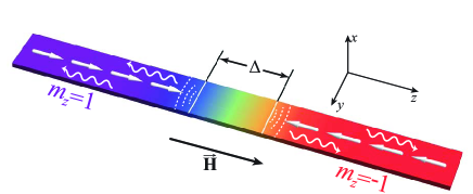
Figure 1: (color online) Schematic of a head-to-head DW of width $\Delta$ in a magnetic nanowire. $\vec{\mathbf{H}}$ is an external field along wire-axis defined as $z$-direction. DW breathing and other types of periodic DW texture deformations emits spin waves, denoted by the wavy lines with arrows.

In this Letter, we numerically solve the LLG equation, initially without damping in order to confirm the above mentioned relation between spin wave emission and DW propagation. Depending on $K_{\perp}$ and the magnetic field, breathing or more complicated periodic transformations of the DW emit spin waves. The DW propagation at low fields tends to lock into a particular soliton mode in which the energy dissipation rate due to the SW emission is balanced by the Zeeman energy gain. We predict robust spin wave emission that persists in the presence of Gilbert damping and renders the usual Walker rigid-body propagation mode unstable in region below the Walker breakdown field.

The LLG equation reads

$$\frac{\partial\mathbf{m}}{\partial t}=-\mathbf{m}\times\mathbf{h}_{\mathrm{eff}}+\alpha\mathbf{m}\times\frac{\partial\mathbf{m}}{\partial t},$$ (1)

where $\mathbf{m}$ is the unit direction of the local magnetization $\mathbf{M}=\mathbf{m}M_{s}$ with saturation magnetization $M_{s}$ and $\alpha$ is the Gilbert damping constant. The effective magnetic field of our biaxial wire (see Fig. 1) is $\mathbf{h}_{\mathrm{eff}}=K_{\parallel}m_{z}\hat{z}-K_{\perp}m_{x}\hat{x}+{A}\partial^{2}\mathbf{m/}\partial{z^{2}}+H\hat{z},$ consisting of internal and external fields in the unit of $M_{s}$. $A$ is the exchange constant. Time, length and energy density are measured in units of $\left(\gamma M_{s}\right)^{-1}$ with gyromagnetic ratio $\gamma$, the DW width at equilibrium $\Delta_{0}=\pi\sqrt{A/K_{\parallel}}$, and $\mu_{0}M_{s}^{2},$ respectively. We chose parameters of the electric insulator Yttrium Iron Garnet (YIG) with magnon ; para $A=3.84\times{10^{-12}}$ $\operatorname{J}/\operatorname{m}$, $K_{\parallel}=2\times 10^{3}$ $\operatorname{J}/\operatorname{m}^{3}$, $\gamma=35.1$ $\operatorname{kHz}/\left(\operatorname{A}/\operatorname{m}\right)$ and $M_{s}=1.94\times 10^{5}$ $\operatorname{A}/\operatorname{m}$, and the corresponding time and length units are $1.46\times 10^{-10}$ $\operatorname{s}$ and $1.38\times 10^{-7}$ $\operatorname{m}$, respectively. $K_{\perp}$ and $\alpha$ are treated as adjustable parameters depending on the sample shape and microscopic order. We solve Eq. (1) by a numerically stable method Algorithm . The mesh size is chosen to be $0.009$, corresponding to the YIG lattice constant ($1.24$ $\operatorname{nm}$).

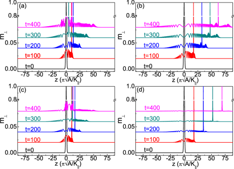
Figure 2: (color online) Snapshots of $m_{\perp}=\sqrt{m_{x}^{2}+m_{y}^{2}}$ for $H=0.01$ at various times $t$ for (a) $K_{\perp}=4$ and $\alpha=0$; (b) $K_{\perp}=10$ and $\alpha=0$; (c) $K_{\perp}=4$ and $\alpha=0.001$; (d) $K_{\perp}=10$ and $\alpha=0.001$.

To prove that a DW under an external field indeed emits spin waves, we plot the snapshots of the distribution of $m_{\perp}\equiv\sqrt{m_{x}^{2}+m_{y}^{2}}$ for $K_{\perp}=4$ and $10$ (in units of $\mu_{0}M_{s}^{2}$), $\alpha=0$, and $H=0.01$ (on at $t=0$) at various times in Figs. 2a and 2b. At $t=0$, right before the external field is switched on, $m_{\perp}$ follows the Walker DW profile Walker , the DW center is located at the center ($z=0$) of a wire with length $180\Delta_{0}$, while the DW magnetization lies in $yz$-plane. Curves are offset for better visibility. As time proceeds ($t>0$), SWs (wavy features) are emitted into both directions, while the DW center (peak) moves simultaneously along the field slower than the SWs. The velocities $v$ for a fixed magnetic field increase monotonically with $K_{\perp}$ (Fig. 3). It does not depend sensitively on small $K_{\perp}\left(<4\right)$, but grows rapidly when $K_{\perp}$ is close to $8$, and becomes an almost linear function of field for $K_{\perp}>12$. From the time-dependence of the position (dashed lines) of DW center and its azimuthal angle (solid lines) shown in the insets of Fig. 3 for a small and large $K_{\perp},$ we trace the periodic DW deformations in the different field regions. We note that such large $K_{\perp}$ value may be realized in YIG samples subject to mechanical strains book .

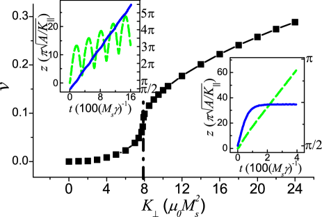
Figure 3: (color online) $K_{\perp}$-dependence of the DW velocity $v$ (in units of $\pi\gamma M_{s}\sqrt{A/K_{\parallel}}$) for fixed $H=0.01$ and $\alpha=0$. Insets: Time dependence of the DW center position (dashed line) and the azimuthal angle $\phi$ (solid line) of magnetization at the DW center for $K_{\perp}=4$ (left) and $K_{\perp}=10$ (right).

At a small $K_{\perp}=4$ (left inset), $\mathbf{m}$ at the DW center rotates around the wire, while the center position oscillates back and forth but also moves slowly along the applied field. This oscillatory motion is synchronized with the breathing, i.e., the periodic energy absorbing and releasing in the form of periodic oscillation of the DW width $\Delta=\pi\sqrt{A/(K_{\parallel}+K_{\perp}\cos^{2}\phi)}$ Walker , where $\phi$ is the tilt angle of the DW plane (with equilibrium value $\pi/2$). This breathing excites spin waves as shown in Fig. 2a. Low velocities corresponds to weak SW emission. At a large $K_{\perp}=10$ (right inset), the azimuthal angle of the DW center approaches a fixed value and the DW center position moves at a constant velocity since $\phi$ and the DW energy are almost constant. In this case, $\mathbf{m}$ still rotates around the wire axis while the DW center propagates along the wire with a fixed $\phi$. The large $K_{\perp}$ twists the DW plane into a chiral screw-like structure that changes shape periodically during the magnetization precession while the DW center “drills” forward. This drilling mode is much more efficient in emitting SWs than the breathing mode, leading to a relatively high DW propagating speed. For YIG parameters the SW velocity exceeds that of the DW, therefore, in contrast to Ref. Wieser , we observe bow as well as stern SW excitations.

Figure 4a displays the steady state DW velocity in a dissipationless wire with $K_{\perp}=4,\ 10,$ and $16$ with parameters otherwise identical to those of Fig. 3. As a function of field it increases abruptly for small values, reaches a maximal value, and decreases again. When $K_{\perp}$ is reduced from 16 to 4 the DW changes from a drilling to the breathing motion, resulting in a significant drop of DW velocity. The decrease of DW velocity with field should not be interpreted as suppression of SW emission or damping of DW propagation by spin wave emission Wieser ; Suhl . The Zeeman energy released by the DW motion at a rate $2HMv$ Wang should be equal to the energy rate carried away by the SWs. Therefore, provided that the latter increases sub-linearly with $H$ ($\propto H^{\beta}$ and $\beta<1$), the DW propagation speed must decrease with field. The initial rapid rise of the DW velocity at small fields is related to the soliton solution $\ln\tan(\theta/2)=\pi(z-vt)/\Delta$ of the LLG Eq. (1) with soliton velocity $v=-\sqrt{A/(K_{\parallel}+K_{\perp}\cos^{2}\phi)}K_{\perp}\sin 2\phi$ for $\alpha=0$ and $H=0$ Braun , where $\theta$ is the polar angle of $\mathbf{m}$. This can be seen from the plot of $-\sin 2\phi$ for the saturated $\phi$ vs. $v\sqrt{(K_{\parallel}+K_{\perp}\cos^{2}\phi)/A}/K_{\perp}$ (symbols) for $H\in[0,0.0009]$ in the inset of Fig. 4a for $K_{\perp}=16$. The numerical data agree precisely with the soliton velocity formula (solid line). Since conventional solitons do not satisfy the LLG equation in the presence of an external field we unearthed here a hybridized mode of solitons and spin waves. In contrast to the zero field case, there is only one particular soliton mode in which the SW emission is balanced by the Zeeman energy change, viz. the moving DW. This holds as long as the field is smaller than the value at which $-\sin 2\phi$ reaches its maximum value 1. Beyond that field, the soliton mode becomes instable since the SW emission rate cannot keep up with the released Zeeman energy and other propagation modes have to take over. This soliton instability point is emphasized by vertical bars in the data points for $K_{\perp}=4$ and $K_{\perp}=10$, indicating the threshold fields below which the soliton formula holds. For $K_{\perp}=16$ this value is out of the range of Fig. 4a.

For YIG parameters and $K_{\perp}=10$, the DW velocity at $H=0.01\left(\sim 24\text{ }\mathrm{Oe}\right)$, is about $140$ $\operatorname{m}/\operatorname{s}$. For comparison, the corresponding DW velocity by Walker rigid body propagation for the same parameters and $\alpha=0.05$ is $57$ $\operatorname{m}/\operatorname{s}$ Walker . We may conclude that the DW velocity in low dissipation magnetic insulators is of the same order of magnitude as in highly dissipative ferromagnetic metals.

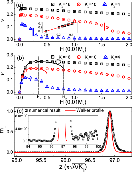
Figure 4: (color online) (a)(b) Field dependence of DW velocity for various $K_{\perp}$. Field and velocity are in units of $0.01M_{s}$ and $\pi\sqrt{A/K_{\parallel}}\gamma M_{s},$ respectively. $A$, $K_{\parallel}$ and $M_{s}$ are YIG parameters. (a) $\alpha=0$. Inset: symbols display $-\sin 2\phi$ vs. $v\sqrt{(K_{\parallel}+K_{\perp}\cos^{2}\phi)/A}/K_{\perp}$, where $v$ is the soliton velocity. The line is the linear relationship from soliton theory. (b) $\alpha=0.001$. The solid curves are the corresponding Walker solutions. (c) Snapshot of $m_{\perp}$ for $H=0.007$ and $K_{\perp}=16$ at $t=400$ (for the datapoint indicated by a circle in (b)). The numerical results deviates from the Walker profile that is clearly narrower. Inset: Expanded view of $m_{\perp}$ close to the DW center. The relative deviation from the Walker profile (solid curve) is pronounced and spin wave emission is conspicuous.

DW propagation through spin wave emission exists in any magnetic wire with transverse magnetic anisotropy irrespective of the Gilbert damping. Figures 2c and 2d look very similar to Figs. 2a and 2b in spite of the finite damping $\alpha=0.001$. Naturally, in the presence of damping the SWs can propagate only over finite distances, which explains why they have been overlooked in most experimental and numerical studies. In Fig. 2b (or 2a) and Fig. 2d (or 2c), the DW velocity is higher in the presence of a small non-zero damping, since damping dissipates an energy on the top of the SW emission and the DW velocity is proportional to the energy dissipation rate Wang . Here we find a mixed DW propagation mode that profits from both Gilbert damping and spin wave emission. Figure 4b is the field dependence of the DW velocity for $\alpha=0.001$ and various $K_{\perp}$, while other model parameters are unmodified from Fig. 4a. Except at very small fields, Fig. 4b is similar with Fig. 4a. The numerically obtained velocities (symbols) in Fig. 4b agree well with Walker’s rigid-body propagation (solid curves) Walker ; Yanming below some maximum field $H_{M}\simeq 2(K_{\parallel}/K_{\perp})^{0.25}H_{W}$ for $K_{\perp}>>K_{\parallel}$, where $H_{W}=\alpha K_{\perp}/2$ Walker is the Walker breakdown field. However, deviations are obvious for fields between $H_{M}$ and $H_{W}$ (where the solid lines end). This implies that Walker rigid-body propagation is not stable for $H\in[H_{M},H_{W}]$ with respect to the spin wave emission mode.

In order to prove numerically that the Walker solution is only stable for $H<H_{M}$, we solve the LLG Eq. (1) starting from an initial magnetization configuration that deviates slightly from the rigid-body propagation mode. The magnetization indeed converges to the Walker profile for $H<H_{M}$. However, this changes when we consider $H=0.007$ for $K_{\perp}=16$ (indicated by dashed circle in Fig. 4b) with all other parameters the same. According to Walker theory Walker , $H_{M}=0.00344$ and $H_{W}=0.008$ (indicated by dashed lines in Fig. 4b). The symbols in Fig. 4c give a snapshot of $m_{\perp}$ for $t=400$, at which the transients die out and the DW center propagates to about $z=97$. The distribution deviates significantly from the Walker profile (solid curve). The spin wave emission is clearly observed in the expanded tail in the inset of Fig. 4c. Exact analytic solutions do not make numerical methods obsolete.

There are several corollaries of the DW propagation mode by spin wave emission. The emitted spin waves from one DW, for example, can mediate an attractive force on the nearby DW, since a DW moves against passing spin waves by spin transfer magnon . This causes crosstalk in wires with more than one domain walls with consequence for the “race track” memory Parkin . This DW-DW attractive force has a finite range governed by the Gilbert damping and is sensitive to material parameters and geometry. The increase of the effective damping by SW emission Suhl is not restricted to DWs but will appear in any time-dependent magnetization texture including magnetic vortices and cannot be captured by the Gilbert phenomenology. On the other hand, our results possibly open alternatives to manipulate and control the effective damping in magnetic nanostructures.

In conclusion, we prove that a DW in a wire with a finite transverse magnetic anisotropy undergoes a periodic transformation under an external magnetic field that excites SWs. The energy carried away must be compensated by the Zeeman energy that is released by DW propagation along the wire. The DW propagation adopts one particular soliton velocity at low fields. This SW assisted DW propagation can be attributed to the SW emission generated by DW breathing and drilling modes. In the presence of damping it competes with and appears before the Walker breakdown. Also, the spin wave emission will mediate a dynamic attractive force between DWs with a range controlled by the Gilbert damping.

This work is supported by Hong Kong UGC/CERG grants (# 604109, HKUST17/CRF/08, and RPC11SC05), the FOM foundation, DFG Priority Program SpinCat, and EG-STREP MACALO.

References

- (1) N.L. Schryer and L.R. Walker, J. Appl. Phys. 45, 5406 (1974).
- (2) D.A. Allwood, G. Xiong, C.C. Faulkner, D. Atkinson, D. Petit, and R.P. Cowburn, Science 309, 1688 (2005).
- (3) G.S.D. Beach, C. Knutson, C. Nistor, M. Tsoi, and J.L. Erskine, Phys. Rev. Lett. 97, 057203 (2006).
- (4) S.S.P. Parkin, M. Hayashi, and L. Thomas, Science 320, 190 (2008).
- (5) G. Malinowski, O. Boulle, and M. Kläui, J. Phys. D: Appl. Phys. 44, 384005 (2011); C.H. Marrows and G. Meier, J. Phys.: Condens. Matter 24, 020301 (2012); G. Tatara, H. Kohno, and J. Shibata, Phys. Rep. 468, 213 (2008).
- (6) R. Nebashi, N. Sakimura, Y. Tsuji, S. Fukami, H. Honjo, S. Saito, S. Miura, N. Ishiwata, K. Kinoshita, T. Hanyu, T. Endoh, N. Kasai, H. Ohno, and T. Sugibayashi, IEEE Symp. VLSI Circuit Dig. Tech. Pap. 300 (2011).
- (7) Z.Z. Sun and X.R. Wang, Phys. Rev. Lett. 97, 077205 (2006); X.R. Wang and Z.Z. Sun, ibid. 98, 077201 (2007).
- (8) H.B. Braun, Adv. Phys. 61, 1 (2012).
- (9) D.S. Han, S.K. Kim, J.Y. Lee, S.J. Hermsoerfer, H. Schutheiss, B. Leven, and B. Hillebrands, Appl. Phys. Lett. 94, 112502 (2009).
- (10) S.M. Seo, H.W. Lee, H. Kohno, and K.J. Lee, Appl. Phys. Lett. 98, 012514 (2011).
- (11) P. Yan, X.S. Wang, and X.R. Wang, Phys. Rev. Lett. 107, 177207 (2011).
- (12) R. Wieser, E.Y. Vedmedenko, and R. Wiesendanger, Phys. Rev. B, 81, 024405 (2010).
- (13) M. Yan, C. Andreas, A. Kákay, F. García-Sánchez, and R. Hertel, Appl. Phys. Lett. 99, 122505 (2011).
- (14) X.R. Wang, P. Yan, J. Lu and C. He, Annals of Physics, 324, 1815 (2009); X.R. Wang, P. Yan, and J. Lu, Europhys. Lett. 86, 67001 (2009).
- (15) H. Kurebayashi, O. Dzyapko, V.E. Demidov, D. Fang, A.J. Ferguson, and S.O. Demokritov, Nat. Mater. 10, 660 (2011).
- (16) X.P. Wang, C.J. García-Cervera, and W. E, J. Comp. Phys. 171, 357 (2001).
- (17) A. Hubert and R. Schäfer, in Magnetic Domains (Springer, Heidelberg, 1998).
- (18) D. Bouzidi and H. Suhl, Phys. Rev. Lett. 65, 002587 (1990).