Enhanced Entrainability of Genetic Oscillators by Period Mismatch

Abstract

Biological oscillators coordinate individual cellular components so that they function coherently and collectively. They are typically composed of multiple feedback loops, and period mismatch is unavoidable in biological implementations. We investigated the advantageous effect of this period mismatch in terms of a synchronization response to external stimuli. Specifically, we considered two fundamental models of genetic circuits: smooth- and relaxation oscillators. Using phase reduction and Floquet multipliers, we numerically analyzed their entrainability under different coupling strengths and period ratios. We found that a period mismatch induces better entrainment in both types of oscillator; the enhancement occurs in the vicinity of the bifurcation on their limit cycles. In the smooth oscillator, the optimal period ratio for the enhancement coincides with the experimentally observed ratio, which suggests biological exploitation of the period mismatch. Although the origin of multiple feedback loops is often explained as a passive mechanism to ensure robustness against perturbation, we study the active benefits of the period mismatch, which include increasing the efficiency of the genetic oscillators. Our findings show a qualitatively different perspective for both the inherent advantages of multiple loops and their essentiality.

I Introduction

Biochemical oscillators exist primarily at the genetic level, such as in the interplay among mRNAs and proteins Novak:2008:BiochemOsc . At least one negative feedback loop (NFL) is essential for limit-cycle oscillation, and in the minimum configuration, one NFL with time-delay is sufficient to generate oscillation. However, many realistic oscillators possess extra components, such as positive feedback loops (PFL) and more than one NFLs, that are apparently redundant. Since more regulatory components consume more resources (e.g., amino acids for synthesis and adenosine triphosphate for operation), this would seem energetically disadvantageous, and thus not preferable through evolution. In addition, the coexistence of positive and negative loops may make the resulting behavior incoherent. Still, the circadian clock of even the simplest life form (e.g., the marine dinoflagellate Gonyaulax polyedra) is composed of multiple oscillators whose rhythms exhibit different periodic patterns Roenneberg:1993:TwoOsc ; Morse:1994:TwoCircadian . Usually this observation is explained by the notion of biological robustness, in which there is a backup mechanism or a resistance to perturbation. However, such observations do not suggest the essentiality of multiple loops: why does not even a single species possess the minimum configuration? In this study, we numerically analyze the inherent advantages of multiple loops from the perspective of entrainment and the adaptation of the system to external input Gonze:2000:Entrainment .

Biologists have investigated coupled oscillators at the molecular level in many different organisms. Bell-Pedersen et al. reviewed circadian clocks in several species from different clades Pederse:2005:MultipleCircadian . They suggested that multiple loops comprise pacemaker and slave oscillators in unicellular organisms, whereas in mammals and avians, a centralized pacemaker entrains downstream systems. Circadian systems have been also investigated theoretically. Wagner et al. studied the stability of an oscillator (called the Goodwin model Goodwin:1965:Oscillator ) against perturbation of the kinetic rate, and found that interlinked loops are more robust (by nearly one order of magnitude) than a non-linked counterpart Wagner:2005:TwoGeneOsc . Other benefits of multiple feedback loops are found in Refs Trane:2007:RobustCircadian ; Hafner:2010:MultiLoop , and their intuitive advantages are summarized in the review by Hastings Hastings:2000:TwoLoopReview .

When multiple loops are involved, synchronization becomes a crucial issue. In biological implementations, no loops can share an identical period in a strict sense. At first glance, such disorder seems to degrade the system performance. However, the results in nonlinear physics indicate that a certain amount of disorder actually enhances performance through mechanisms similar to those in stochastic resonance Benzi:1981:SR ; McNamara:1989:SR ; Jung:1991:AmpSR ; Jung:1992:GlobalSR ; Gammaitoni:1998:SR ; McDonnell:2008:SRBook ; McDonnell:2009:SR ; Hasegawa:2011:BistableSIN , Brownian transport Astumian:1994:MolecularMotor ; Astumian:1997:BrownMotor ; Frey:2005:BrownianRev ; Hanggi:2009:BrownianMotorsReview ; Hasegawa:2012:Motor , noise-induced synchronization Marchesoni:1996:SpatiotempSR ; Nakao:2007:NISinLC ; Teramae:2004:NoiseIndSync , and disorder-induced resonance Tessone:2006:DiversityResonance .

Our focus is the property called entrainability, or the ability of oscillators to be synchronized with an external periodic signal. It is directly connected to the adaptability of the species and therefore its survival Sharma:2003:CircadianAdaptive . Not only does a Drosophila with a circadian clock survive better than one without  Beaver:2002:FlyClock , but also an Arabidopsis with better entrainment with the environment has increased photosynthesis and consequently grows faster Dodd:2005:PlantCircadian . Even cyanobacteria with better entrainability have an advantage over nonsynchronizable ones, although this advantage disappears in constant environments Woelfle:2004:CyanoClock .

At the molecular level, entrainability has been attributed to several different mechanisms. Gonze et al. studied a population of suprachiasmatic nuclei (SCN) neurons and showed that efficient global synchronization is achieved via damping Gonze:2005:CircadianSync . Liu et al. experimentally confirmed that robust oscillatory behavior can be achieved by tissue-level communication between SCN cells, even if critical clock genes have been knocked out  Liu:2007:Cell . Tsai et al. reported that the presence of PFLs allowed for easier tuning of the period without changing the amplitude Tony:2008:TunablePositive . Zhou et al. showed that positive feedback loops assist noise-induced synchronization through their sensitivity to external signals Zhou:2008:SyncGeneOsc .

Still, a fundamental question has not been answered: what is the advantage of harboring multiple loops with mismatched periods? We investigate the effects of mismatched periods on limit-cycle oscillations from the viewpoint of entrainment. Specifically, we consider the minimal fundamental model: an oscillator made of two loops, each of a different period, that are connected. By using phase reduction and Floquet multipliers, we analyzed the response of this system to external periodic stimuli as a function of the coupling strength and the period ratio. Our main finding is the large effect of mismatched periods on entrainability: that is, better entrainment is achieved when the two oscillatory components have different natural periods. This enhancement effect is observed in two types of coupled oscillators: smooth and relaxation oscillators (Figure 1). The enhanced entrainability seen in the present study is similar to that reported by Komin et al. Komin:2010:EntrainCircadian . However, our mechanism is different from theirs: the enhancement in our case is caused by the oscillators in the vicinity of the bifurcation on the limit cycle whereas their enhancement results from damped oscillation (oscillator death).

II Methods

We studied the effects of mismatched periods on entrainment by using smooth and relaxation oscillators. Before explaining the details of these models, we will first explain period scaling and a coupling scheme.

II.1 The base model

An $N$-dimensional differential equation for a single oscillator is represented by

$$\frac{d\boldsymbol{v}}{dt}=\boldsymbol{f}(\boldsymbol{v}),$$ (1)

where $\boldsymbol{v}$ and $\boldsymbol{f}(\boldsymbol{v})$ are $N$-dimensional column vectors defined by

$$\boldsymbol{v}=(x,y,z,\cdots)^{\top},\hskip 10.00002pt\boldsymbol{f}(\boldsymbol{v})=(f_{1}(\boldsymbol{v}),f_{2}(\boldsymbol{v}),\cdots,f_{N}(\boldsymbol{v}))^{\top},$$

where $\top$ denotes a transposed vector (matrix). Equation 1 yields autonomous oscillation (a limit-cycle oscillation) whose period is $T$. The period can be tuned without changing the amplitude of the oscillation by introducing a scaling parameter $\tau$

$$\frac{d\boldsymbol{v}}{dt}=\frac{\boldsymbol{f}(\boldsymbol{v})}{\tau},$$ (2)

where the period of equation 2 is given by $\tau T$. Other than their periods, solutions to equation 2 with different $\tau$ values will have the same properties Gonze:2005:CircadianSync ; Komin:2010:EntrainCircadian . We used equation 2 to study the effects of mismatched periods between two oscillatory components:

$$\frac{d\boldsymbol{v}_{1}}{dt} = \frac{\boldsymbol{f}(\boldsymbol{v}_{1})}{\tau_{1}}+\boldsymbol{C}_{1}(\boldsymbol{v}_{1},\boldsymbol{v}_{2}),$$ (3)

$$\frac{d\boldsymbol{v}_{2}}{dt} = \frac{\boldsymbol{f}(\boldsymbol{v}_{2})}{\tau_{2}}+\boldsymbol{C}_{2}(\boldsymbol{v}_{2},\boldsymbol{v}_{1}),$$ (4)

where the subscript $i$ denotes the $i$th component and $\boldsymbol{C}_{i}(\boldsymbol{v}_{i},\boldsymbol{v}_{j})$ represents a coupling term. To investigate the effects of mismatched periods, we set

$$\tau_{1}=1,\hskip 10.00002pt\tau_{2}=R,$$ (5)

where $R$ represents the ratio of the periods of the two oscillators.

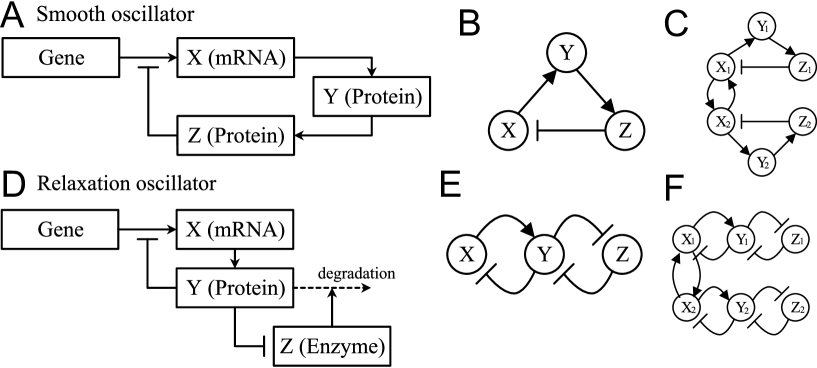
Figure 1: (A) Diagram of a smooth oscillator, (B) simplified diagram of a single smooth oscillator, (C) two coupled smooth oscillators, (D) diagram of a relaxation oscillator, (E) simplified diagram of a single relaxation oscillator, and (F) two coupled relaxation oscillators. The symbols $\rightarrow$ and $\dashv$ represent positive and negative regulations, respectively.

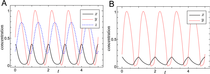
Figure 2: Time courses of (A) the smooth oscillator (equation 6) and (B) the relaxation oscillator (equation 8). Solid, dotted, and dashed lines denote $x$, $y$, and $z$, respectively. The period and the amplitude of $y$ are normalized to $1$ in both models.

II.2 Genetic oscillator models

We show two specific models of $\boldsymbol{f}(\boldsymbol{v})$, each for the smooth and relaxation oscillators.

II.2.1 Smooth oscillator

A smooth oscillator is the most basic structure for limit-cycle oscillations Novak:2008:BiochemOsc , and many biochemical oscillators (e.g., the Goodwin model Goodwin:1965:Oscillator and the repressilator Elowitz:2000:Repressilator ) belong to this class. We adopted the smooth oscillator presented in Novák and Tyson Novak:2008:BiochemOsc (Figure 1). A diagram and the simplified structure of the smooth oscillator are shown in Figures 1A and B, where the transcription of $X$ (mRNA) is inhibited by $Z$ (protein). Protein $Y$ plays a role in the time-delay of the loop $X\rightarrow Y\rightarrow Z\dashv X$, where $X\rightarrow Y$ and $X\dashv Y$ denote activation and repression, respectively. In the presence of sufficient time delay in the NFL, the regulatory network exhibits limit-cycle oscillations. The dynamics of the smooth oscillator are described by the following three-dimensional differential equation on $\boldsymbol{v}=(x,y,z)^{\top}$, where $x$, $y$, and $z$ denote the concentrations of mRNA $X$, protein $Y$, and protein $Z$, respectively:

$$\boldsymbol{f}(\boldsymbol{v})=\left(\begin{array}[]{c}{\displaystyle V_{sx}\frac{K_{d}^{p}}{K_{d}^{p}+z^{p}}-k_{dx}x}\\ {\displaystyle k_{sy}x-V_{dy}\frac{y}{K_{m}+y}}\\ k_{sz}y-k_{dz}z\end{array}\right).$$ (6)

Because the amplitude and the period of the limit cycle can be tuned separately by proper scaling, we employed the parameters $V_{sx}=5.44$, $k_{dx}=8.99$, $k_{sz}=4.49$, $k_{dz}=4.49$, $k_{sy}=18.0$, $V_{dy}=2.72$, $K_{m}=0.00303$, $K_{d}=0.303$, and $p=4.0$ to achieve unit period and unit amplitude for $y$ (we define the amplitude as the difference between the maximum and the minimum of the oscillation. See Figure 2A). These parameter settings are essentially identical to those presented in the Supplement of Novák and Tyson Novak:2008:BiochemOsc , except for the scale transform ($V_{sx}=0.2$, $k_{dx}=0.1$, $k_{sz}=0.05$, $k_{dz}=0.05$, $k_{sy}=0.2$, $V_{dy}=0.1$, $K_{m}=0.01$, $K_{d}=1.0$, and $p=4.0$ in the original model).

We analyzed two coupled smooth oscillators, as shown in Figure 1C, where the subscript $i$ of $X_{i}$ denotes the $i$th oscillator component. We assumed that the protein translated from $X_{1}$ positively regulates the transcription of $X_{2}$. The coupling term in equations 3 and 4 can be written in the following linear relation:

$$\boldsymbol{C}_{i}(\boldsymbol{v}_{i},\boldsymbol{v}_{j})=\left(\begin{array}[]{c}\epsilon(x_{j}-x_{i})\\ 0\\ 0\end{array}\right)\hskip 10.00002pt((i,j)=(1,2)\,\,\mathrm{or}\,\,(2,1)),$$ (7)

where $\epsilon$ denotes the coupling strength.

II.2.2 Relaxation oscillator

The existence of PFLs makes oscillators excitatory, and such oscillators are known as relaxation oscillators Novak:2008:BiochemOsc . Relaxation oscillators have cusps in their nullcline curves, and one example of this class is the FitzHugh–Nagumo oscillator FitzHugh:1961:FHmodel ; Nagumo:1962:NagumoModel .

We again employ a relaxation-type genetic oscillator presented by Novák and Tyson Novak:2008:BiochemOsc . Figures 1D and E show specific and simplified models, respectively, of a relaxation oscillator in which transcription of $X$ (mRNA) is inhibited by $Y$ (protein), which serves as a NFL. Following this, $Y$ (mRNA) is degraded by $Z$ (enzyme) and also forms an enzyme-substrate complex $ZY$ to inhibit the functionality of $Z$ ($ZY+Y\rightleftharpoons ZYY$). The interaction $Y\dashv Z\dashv Y$ functions as the PFL in this network. In many cases, it is assumed that the concentration of enzyme $Z$ equilibrates ($\dot{z}=0$), yielding the following two-dimensional differential equation in terms of $\boldsymbol{v}=(x,y)^{\top}$, where $x$ and $y$ denote the concentrations of mRNA $X$ and protein $Y$, respectively:

$$\boldsymbol{f}(\boldsymbol{v})=\left(\begin{array}[]{c}{\displaystyle V_{sx}\frac{K_{d}^{p}}{K_{d}^{p}+y^{p}}-k_{dx}x}\\ {\displaystyle k_{sy}x-k_{dy}y-V_{dy}\frac{y}{K_{m}+y+y^{2}/K_{1}}}\end{array}\right).$$ (8)

As in the smooth oscillator, we scaled the parameters so that the period and the amplitude $y$ both became $1$ (Figure 2B). The parameters, $V_{sx}=0.815$, $K_{m}=0.0268$, $k_{dx}=3.04$, $k_{sy}=60.8$, $k_{dy}=3.04$, $V_{dy}=16.3$, $K_{1}=0.134$, $K_{d}=0.268$, and $p=4.0$, are essentially equivalent to those presented in the Supplement of Novák and Tyson Novak:2008:BiochemOsc , except for the scale transform ($V_{sx}=0.05$, $K_{m}=0.1$, $k_{dx}=0.05$, $k_{sy}=1.0$, $k_{dy}=0.05$, $V_{dy}=1.0$, $K_{1}=0.5$, $K_{d}=1.0$, and $p=4.0$ in the original model).

We analyzed two coupled relaxation oscillators, as shown in Figure 1F. The coupling term $\boldsymbol{C}_{i}$ was written as a linear relation:

$$\boldsymbol{C}_{i}(\boldsymbol{v}_{i},\boldsymbol{v}_{j})=\left(\begin{array}[]{c}\epsilon(x_{j}-x_{i})\\ 0\end{array}\right)\hskip 10.00002pt((i,j)=(1,2)\,\,\mathrm{or}\,\,(2,1)),$$ (9)

where $\epsilon$ denotes the coupling strength.

II.3 Analytical approaches

For an analytical analysis, we used phase reduction and Floquet multipliers. Even a system of only two coupled oscillators exhibits very complicated behaviors, such as $n:m$ synchronization ($n,m$; positive integers) and chaos, depending on the model parameters (see section III). Because detailed bifurcation analysis of the coupled oscillator is outside the scope of this paper, we assumed $1:1$ synchronization between two oscillatory components (tight coupling). Under this assumption, the coupled oscillator can be viewed as one oscillator, whose dynamics is represented by

$$\frac{d\boldsymbol{u}}{dt}=\boldsymbol{g}(\boldsymbol{u}),$$ (10)

with

$$\boldsymbol{u}=\left(\begin{array}[]{c}\boldsymbol{v}_{1}\\ \boldsymbol{v}_{2}\end{array}\right),\hskip 10.00002pt\boldsymbol{g}(\boldsymbol{u})=\left(\begin{array}[]{c}{\displaystyle\frac{\boldsymbol{f}(\boldsymbol{v}_{1})}{\tau_{1}}+\boldsymbol{C}_{1}(\boldsymbol{v}_{1},\boldsymbol{v}_{2})}\\ {\displaystyle\frac{\boldsymbol{f}(\boldsymbol{v}_{2})}{\tau_{2}}+\boldsymbol{C}_{2}(\boldsymbol{v}_{2},\boldsymbol{v}_{1})}\end{array}\right).$$ (11)

Incorporating an input signal in equation 10, we have

$$\frac{d\boldsymbol{u}}{dt}=\boldsymbol{g}(\boldsymbol{u})+\chi\boldsymbol{I}(\omega t),$$ (12)

where $\boldsymbol{I}(\omega t)$ denotes an input signal with angular frequency $\omega$ and $\chi$ is a scalar representing the signal strength. We will use equation 12 in the calculations for entrainability and Floquet multipliers.

II.3.1 Phase reduction

A phase-reduction approach uses a phase variable to reduce a multidimensional system into a one-dimensional differential equation Kuramoto:2003:OscBook ; Izhikevich:2007:NeuroBook . In the absence of external perturbations (equation 10), a limit-cycle oscillation can be described in terms of a phase variable $\phi\in[0,2\pi]$:

$$\frac{d\phi}{dt}=\Omega,$$ (13)

where $\Omega$ is the natural angular frequency of the limit cycle ($\Omega=2\pi/T$, where $T$ is the period). Although the phase $\phi$ in equation 13 is only defined on the stable limit-cycle trajectory, its definition can be expanded to the entire $\boldsymbol{u}$ space, where the equiphase surface is called the isochron $\mathcal{I}(\phi)$. An example of an isochron $\mathcal{I}(\phi)$ defined on a hypothetical limit-cycle oscillator, shown by dashed lines, in Figure 3A where the isochron is drawn at intervals of $\pi/6$.

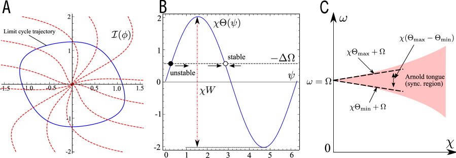
Figure 3: (A) Trajectory of a hypothetical limit-cycle oscillator (solid line) and its isochron $\mathcal{I}(\phi)$ (dashed lines), where the isochron is drawn at intervals of $\pi/6$. (B) Illustration of $\dot{\psi}=\Delta\Omega+\chi\Theta(\psi)=0$, where the solid and dashed line denote $\chi\Theta(\psi)$ and $-\Delta\Omega$, respectively, for typical cases. A stable solution (empty circle) exists inside $\chi\Theta_{\max}$ and $\chi\Theta_{\min}$, whose length is denoted by $\chi W$. (C) Illustration of the relation between the Arnold tongue (colored region), inside which the oscillator can synchronize to an external signal (vertical and horizontal axes represent the signal angular frequency $\omega$ and the signal strength $\chi$, respectively). Equation 19 (dashed line) is a linear approximation of this region for sufficiently small $\chi$. The width of the region can be approximated by $\chi(\Theta_{\max}-\Theta_{\min})$ around $\chi=0$.

In the presence of external signals (equation 12), the time evolution of $\phi$ is described by

$$\frac{d\phi}{dt}=\Omega+\chi\boldsymbol{U}(\phi)\cdot\boldsymbol{I}(\omega t),$$ (14)

where a dot ($\cdot$) represents an inner product and $\boldsymbol{U}(\phi)$ is the phase response curve (PRC) defined by

$$\boldsymbol{U}(\phi^{\prime})=\left.\nabla\phi(\boldsymbol{u})\right|_{\boldsymbol{u}=\boldsymbol{u}_{0}(\phi^{\prime})}.$$ (15)

Here $\boldsymbol{u}_{0}(\phi^{\prime})$ represents a point on limit-cycle oscillation at the phase $\phi^{\prime}$. It is assumed that the perturbed trajectory is in the vicinity of the unperturbed limit-cycle trajectory (i.e., $\chi$ is sufficiently small). The introduction of a slow variable $\psi=\phi-\omega t$ in equation 14 yields

$$\frac{d\psi}{dt}=\Delta\Omega+\chi\boldsymbol{U}(\psi+\omega t)\cdot\boldsymbol{I}(\omega t),$$ (16)

where $\Delta\Omega=\Omega-\omega$. Because $\psi$ is a slow variable ($\dot{\psi}$ is very small), when $\chi$ is sufficiently small, the inner product term can be approximated by its average (separating the timescales of $\psi$ and $\boldsymbol{U}(\psi+\omega t)\cdot\boldsymbol{I}(\omega t)$):

$$\frac{d\psi}{dt} \simeq \Delta\Omega+\chi\Theta(\psi),$$ (17)

with

$$\Theta(\psi)=\frac{1}{2\pi}\int_{0}^{2\pi}d\theta\,\boldsymbol{U}(\psi+\theta)\cdot\boldsymbol{I}(\theta),$$ (18)

(the integration of equation 18 is evaluated numerically in practical calculations). If stable solutions exist, this oscillator synchronizes to external signals. $\Theta(\psi)$ is a $2\pi$-periodic function, and its shape is typically given by sinusoidal-like functions, as shown in Figure 3B. The fixed points are the intersection points of $\Theta(\psi)$ and $-\Delta\Omega$, and only the point with $\frac{d\Theta}{d\psi}<0$ is a stable solution (an empty circle in Figure 3B). Therefore, the oscillator is synchronized to external signals if the following relation holds:

$$\chi\Theta_{\min}+\Omega<\omega<\chi\Theta_{\max}+\Omega,$$ (19)

with

$$\Theta_{\min}=\min_{\psi}\Theta(\psi),\hskip 10.00002pt\Theta_{\max}=\max_{\psi}\Theta(\psi).$$

The extent of synchronization in terms of $\chi$ (signal strength) and $\omega$ (signal angular frequency) is often described by a domain known as the Arnold tongue or the synchronization region Pikovsky:2001:SyncBook , inside of which the oscillator can synchronize to an external periodic signal (the colored domain in Figure 3C). Although the border of the Arnold tongue is generally nonlinear as a function of $\chi$, the upper and lower borders can be approximated linearly by equation 19 when $\chi$ is sufficiently small (these are shown with the dashed line in Figure 3C). Thus the range in which $\omega$ can be synchronized with an external signal can be quantified by $\chi(\Theta_{\max}-\Theta_{\min})$, which represents the width of the Arnold tongue for sufficiently small $\chi$. We define the entrainability $W$ as a $\chi$-independent variable (see Figure 3B):

$$W=\Theta_{\max}-\Theta_{\min}.$$ (20)

Writing equation 19 in terms of the period of the external signal, we have

$$\frac{2\pi}{\chi\Theta_{\max}+\Omega}<T_{s}<\frac{2\pi}{\chi\Theta_{\min}+\Omega},$$ (21)

where $T_{s}$ is the period of the external signal ($T_{s}=2\pi/\omega$) (note that equations 19 and 21 only hold for sufficiently small $\chi$). The PRC [equation 15] can be calculated by the following differential equation Izhikevich:2007:NeuroBook ; Shwemmer:2012:WeaklyCoupleOsc :

$$\frac{d\boldsymbol{U}(t)}{dt}=-\left\{D\boldsymbol{g}(\boldsymbol{u}_{0}(t))\right\}^{\top}\boldsymbol{U}(t),$$ (22)

with the constraint

$$\boldsymbol{U}(t)\cdot\boldsymbol{g}(\boldsymbol{u}_{0}(t))=\Omega,$$ (23)

where $\boldsymbol{u}_{0}(t)$ is a stable periodic solution of equation 10 ($\boldsymbol{u}_{0}(t+T)=\boldsymbol{u}_{0}(t)$, where $T$ is the period), $D\boldsymbol{g}(\boldsymbol{u}_{0}(t))$ is a Jacobian matrix of $\boldsymbol{g}(\boldsymbol{u})$ around $\boldsymbol{u}_{0}(t)$, and we abbreviated $\boldsymbol{U}(t)=\boldsymbol{U}(\phi(t))$ ($\phi(t)$ is the phase as a function of $t$ according to equation 13). Because equation 22 is unstable, we numerically solved equation 22 backward in time.

II.3.2 Floquet multiplier

In the presence of external signals, the solution $\boldsymbol{u}(t)$ deviates from a stable orbit $\boldsymbol{u}_{0}$, where the deviation $\boldsymbol{\eta}=\boldsymbol{u}-\boldsymbol{u}_{0}$ obeys the differential equation

$$\frac{d\boldsymbol{\eta}(t)}{dt}=D\boldsymbol{g}(\boldsymbol{u}_{0}(t))\boldsymbol{\eta}(t).$$ (24)

Here we assume that the deviation is sufficiently small. Because $D\boldsymbol{g}(\boldsymbol{u}_{0})$ is a periodic function with period $T$, equation 24 has the Floquet solutions, generally represented by

$$\boldsymbol{\eta}(t)=\sum_{i=1}^{N}c_{i}\exp(\mu_{i}t)\boldsymbol{p}_{i}(t),$$ (25)

where $\boldsymbol{p}_{i}(t)$ are functions with period $T$, $c_{i}$ is a coefficient determined by the initial conditions, and $\mu_{i}$ are the Floquet exponents. The Floquet multipliers $\rho_{i}$ are related to the exponents via

$$\rho_{i}=\exp(\mu_{i}T).$$ (26)

Note that the Floquet exponents are a special case of the Lyapunov exponents for periodic systems (e.g., limit cycles) Klausmeier:2008:Floquet . The Floquet multipliers can be calculated numerically from a matrix differential equation in terms of the matrix $Q(t)$, after Klausmeier Klausmeier:2008:Floquet :

$$\frac{dQ(t)}{dt}=D\boldsymbol{g}(\boldsymbol{u}_{0}(t))Q(t).$$ (27)

Equation 27 is integrated numerically from $t=0$ to $t=T$ with an initial condition that $Q(t=0)$ is the identity matrix. The Floquet multipliers are obtained as the eigenvalues of $Q(t=T)$, and hence $N$-dimensional limit-cycle models yield $N$ Floquet multipliers.

When the Floquet multipliers $\rho_{i}$ cross the unit circle $|\rho|=1$ on the complex plane, the limit cycle bifurcates. Bifurcations of codimension 1 can occur in three patterns Guckenheimer:1983:DynsysBook ; Crawford:1991:IntroBifTheory ; Wiesenfeld:1985:PDBifAmp ; Wiesenfeld:1986:SignalAmpBif :

• Saddle-node bifurcation: A single real Floquet multiplier crosses $\rho=1$ (this includes transcritical or pitchfork bifurcations as special cases);

• Hopf bifurcation: Complex-conjugate Floquet multipliers cross $\left|\rho\right|=1$ ($\rho\neq\pm 1$);

• Period-doubling bifurcation: A single real Floquet multiplier crosses $\rho=-1$.

In autonomous systems, one of the Floquet multipliers is $\rho_{i}=1$, which corresponds to a pure phase shift. Wiesenfeld and McNamara showed that Floquet multipliers whose absolute values are close to 1 are responsible for signal amplification Wiesenfeld:1985:PDBifAmp ; Wiesenfeld:1986:SignalAmpBif . We calculated the Floquet multipliers up to the second-largest absolute value (except for the inherent multiplier $\rho=1$), which are denoted as $\rho_{1}$ (the largest) and $\rho_{2}$ (the second largest) in our models.

III Results

We performed a bifurcation analysis and examined the relationship between entrainability and the Floquet multipliers. We set $\tau_{1}=1$ and $\tau_{2}=R$ in equations 3 and 4, where $R$ represents the ratio of the periods of the two oscillators. When $R\neq 1$, the two oscillatory components have different natural periods (without coupling) and hence the periods are mismatched. As the controllable parameters for the model calculations, we adopted $R$ and $\epsilon$, where $\epsilon$ denotes the coupling strength defined in equations 7 and 9.

III.1 Bifurcation diagram

Bifurcations of the limit cycle are classified into bifurcations in equilibria and those on the limit cycle. Here, bifurcation on the limit cycle was studied by numerically solving differential equations 6 and 8.

Specifically, we described the bifurcation diagrams as a function of $R$ (period ratio) and $\epsilon$ (coupling strength) and calculated the local maxima of $y_{1}$. If the oscillator showed regular limit-cycle oscillations, the maxima of $y_{1}$ was represented by a single point. If the limit cycle underwent bifurcation, the maximal points were described by more than two points. We iterated by changing $R$ from $R_{\min}$ to $R_{\max}$ ($R_{\min}<R_{\max}$) and then adopted the last values of the preceding $R$ values as the initial values for the next $R$ value. The incremental step for $R$ was set at $\Delta R=(R_{\max}-R_{\min})/1000$, where $R_{\min}$ and $R_{\max}$ are indicated as the lower and upper limits on Figures 4 and 6. At each parameter value, we discarded as transient phases those during $t\in[0,200]$, and we recorded the local maxima of the trajectories in during the intervals $t\in[200,300]$. We carried out these same procedures on the coupling parameter $\epsilon$ ($\epsilon_{\min}$, $\epsilon_{\max}$, with the increment $\Delta\epsilon=(\epsilon_{\max}-\epsilon_{\min})/1000$).

In Figure 4, the bifurcation diagram of $y_{1}$ as a function of $R$ in the smooth oscillator is shown for (A) $\epsilon=1.5$ and (B) $\epsilon=2.5$. Although the maxima of $y_{1}$ slightly depend on $R$, there is no bifurcation. In Figure 5, the bifurcation diagram as a function of $\epsilon$ is shown for (A) $R=1.4$ and (B) $R=2.5$. In both cases, bifurcations occurred at $\epsilon\simeq 1.3$ for $R=1.4$ and $\epsilon\simeq 0.9$ for $R=2.5$, and chaotic behavior was observed when the coupling strength was small.

Figure 6 shows the bifurcation diagram as a function of $R$ for the relaxation oscillator for (A) $\epsilon=2.0$ and (B) $\epsilon=2.5$. In the former case, a period-doubling bifurcation occurred in the region $1.7<R<2.7$. In the latter, a cusp appeared around $R=1.9$, in the vicinity of a saddle-node bifurcation (see the section on entrainability and Floquet multipliers). In Figure 7, the bifurcation diagram as a function of $\epsilon$ is shown for (A) $R=1.3$ and (B) $R=1.9$. A complex behavior (chaos) appeared in a small region of $\epsilon$. Especially in Figure 7B, we found a branch of a maxima around $1.7<\epsilon<2.3$, indicating the occurrence of the period-doubling bifurcation.

In comparison, bifurcations are less likely in a smooth oscillator than in a relaxation oscillator; bifurcations are only observed in the case of very weak coupling in smooth oscillators (Figure 5). In contrast, the relaxation oscillator exhibited period-doubling and chaotic oscillations in a wider range of coupling strengths (Figures  6 and 7).

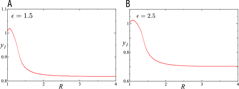
Figure 4: Bifurcation diagram (local maxima of $y_{1}$) of the smooth oscillator as a function of $R$, where (A) $\epsilon=1.5$, and (B) $\epsilon=2.5$.

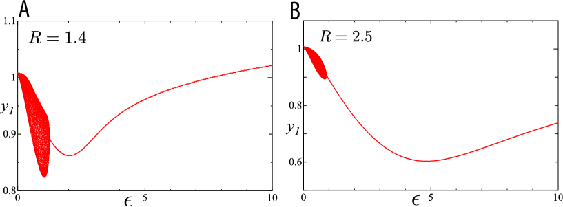
Figure 5: Bifurcation diagram (local maxima of $y_{1}$) of the smooth oscillator as a function of $\epsilon$, where (A) $R=1.4$, and (B) $R=2.5$.

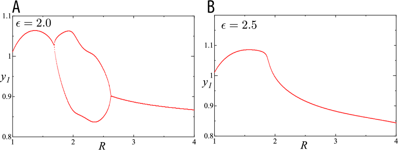
Figure 6: Bifurcation diagram (local maxima of $y_{1}$) of the relaxation oscillator as a function of $R$, where (A) $\epsilon=2.0$, and (B) $\epsilon=2.5$.

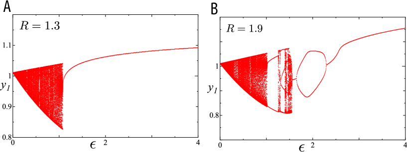
Figure 7: Bifurcation diagram (local maxima of $y_{1}$) of the relaxation oscillator as a function of $\epsilon$, where (A) $R=1.3$, and (B) $R=1.9$.

Next, we examine the time course of the coupled oscillators with mismatched periods (Figures 8 and 9, respectively, for the smooth and relaxation oscillators). Without mismatched periods, the temporal trajectory of the oscillators would be identical to that of the case of a single oscillator (Figure 2). Figure 8 shows the case for coupled smooth oscillators with (A) $\epsilon=1.5$, $R=1.5$, and (B) $\epsilon=2.5$, $R=1.5$; Figure 9 shows the case for coupled relaxation oscillators with (A) $\epsilon=2.0$, $R=2.8$, and (B) $\epsilon=2.5$, $R=1.9$. In all the cases shown in Figures 8 and 9, we see the $1:1$ synchronization between the two oscillators. Without period mismatch, the amplitude of oscillation $y$ is $1$ (see Methods). We see from Figures 8 and 9 that the amplitudes of $y_{1}$ and $y_{2}$ depend on the period ratio $R$, where the amplitude of $y_{1}$ is smaller than 1 except in Figure 9B. From Figures 4 and 6, which describe maxima of $y_{1}$ as a function $R$, we see that $y_{1}$ is larger than 1 in both oscillator models when the period mismatch is smaller, and the maxima of $y_{1}$ start to decrease with increasing $R$. The decrease of the amplitude is larger for the smooth oscillator than for the relaxation oscillator.

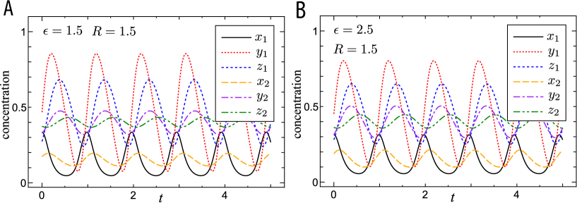
Figure 8: Time course of the coupled smooth oscillator with (A) $\epsilon=1.5$ and $R=1.5$, and (B) $\epsilon=2.5$ and $R=1.5$.

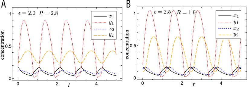
Figure 9: Time course of the coupled relaxation oscillator, with (A) $\epsilon=2.0$ and $R=2.8$, and (B) $\epsilon=2.5$ and $R=1.9$.

III.2 Entrainability and Floquet multiplier

In using phase reduction and Floquet multipliers to calculate how the entrainability $W$ (equation 20) depends on $R$ (equation 5) and $\epsilon$ (equations 7 and 9), we employed the following sinusoidal input signal:

$$\boldsymbol{I}(\omega t)=\left(\begin{array}[]{c}\sin(\omega t)\\ 0\\ 0\\ \vdots\end{array}\right),$$ (28)

where the input signal only affects the concentration of mRNA in the first oscillator ($x_{1}$ in equation 10). We assumed $1:1$ synchronization between the two oscillators (the regions where the maximum of $y_{1}$ is represented by a single point in Figures 4–7) so that the coupled oscillator could be viewed as a single case. Although we calculated the entrainability and the Floquet multipliers inside the $1:1$ synchronized regions, the entrainability very close to the bifurcation points is not shown for some parameters, because equation 22 did not exhibit stable periodic solutions even after remaining there for a long time ($\epsilon\simeq 1.3$ in Figure 11A, $R\simeq 2.7$ in Figure 12A and $\epsilon\simeq 2.3$ in Figure 13D). In most cases we calculated the Floquet multipliers up to the second most dominant ones. When the multipliers were given by complex-conjugate values, we checked the three multipliers $\rho_{1}$, $\bar{\rho}_{1}$, and $\rho_{2}$, where $\bar{\rho}$ is the complex conjugate of $\rho$. When two real multipliers ($\rho_{1}$ and $\rho_{1}^{\prime}$) eventually emerged due to annihilation of the complex-conjugate multipliers ($\rho_{1}$ and $\bar{\rho}_{1}$) by changing parameters, we checked the three multipliers $\rho_{1}$, $\rho_{1}^{\prime}$, and $\rho_{2}$.

By calculating the entrainability $W$ and the Floquet multipliers $\rho_{i}$, we obtained stable limit-cycle trajectories in a way similar to what we did in the bifurcation analysis. We iterated over $R$ and adopted the values of the preceding $R$ values as the initial values for the next $R$ values. For each parameter value, we calculated the stable limit-cycle trajectories for one period, and these trajectories were used for the calculation of the PRC functions (Equation 15). These procedures were also carried out for the coupling parameter $\epsilon$. The Floquet multipliers also require stable limit-cycle trajectories, and we calculated them in the same way as described above.

III.2.1 Smooth oscillator

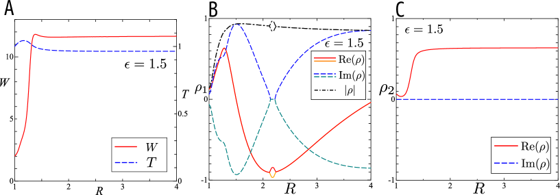
Figure 10: Entrainability $W$, period $T$, and Floquet multipliers $\rho_{i}$, as a function of $R$ in the smooth oscillator. (A–C) $R$ dependence of (A) $W$ and $T$, (B) $\rho_{1}$, and (C) $\rho_{2}$, for $\epsilon=1.5$. In (A), the solid and dashed lines denote the entrainability and the period, respectively. In B and C, the solid, dashed, and dot-dashed lines denote the real part, the imaginary part, and absolute value of the Floquet multipliers, respectively.

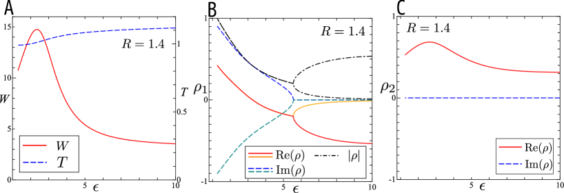
Figure 11: Entrainability $W$, period $T$, and Floquet multipliers $\rho_{i}$, as a function of $\epsilon$ in the smooth oscillator. (A–C) $\epsilon$ dependence of (A) $W$ and $T$, (B) $\rho_{1}$, and (C) $\rho_{2}$, for $R=1.4$. The meanings of the lines are the same as in Figure 10.

We first investigated the smooth oscillator as a function of $R$ (Figure 10). Specifically, Figure 10A is a dual-axis plot of the entrainability $W$ (solid line; left axis) and the period $T$ (dashed line; right axis) for $\epsilon=1.5$. We can uniquely define the period $T$ of the coupled oscillator because we are considering a $1:1$ synchronization between the two oscillators. In Figure 10A, the period $T$ is not strongly affected by period mismatch and is around $1$ in the whole $R$ region, although the entrainability $W$ depends on $R$. The entrainability is $W\simeq 2$ when the two oscillators have the same period ($R=1$), whereas $W\simeq 12$ for $R\geq 1.4$. The first and the second dominant Floquet multipliers for $\epsilon=1.5$ are shown in Figure 10B and C, where solid, dashed, and dot-dashed lines respectively denote $\mathrm{Re}(\rho_{i})$, $\mathrm{Im}(\rho_{i})$, and $|\rho_{i}|$ ($\rho_{i}$: Floquet multiplier defined by equation 26). In Figure 10B, symmetric imaginary curves represent complex-conjugate multipliers, and a branch of the real part around $R\simeq 2.2$ is due to annihilation of the complex-conjugate multipliers (two real multipliers emerge in place of the complex-conjugate multipliers). We see that the $\rho_{1}$ in Figure 10B are imaginary values, and their absolute values are close to 1 for the $R>1.4$ region. The coupled oscillator is close to the Hopf bifurcation points. The second dominant Floquet multiplier $\rho_{2}$ is described in Figure 10C, and we see that its magnitude is comparable to that of $\rho_{1}$. The coupled oscillator is near the saddle-node bifurcation points (the second Floquet multiplier $\rho_{2}$ is a pure real value). We also carried out the same calculations with $\epsilon=2.5$ and found enhanced entrainability $W\simeq 16$ in the presence of a period mismatch ($R>1.5$), as in Figure 10C (data not shown). According to the analysis with Floquet multipliers, this enhancement can also be accounted for by the bifurcation.

Figure 11 shows the entrainability and Floquet multipliers as a function of $\epsilon$ in the smooth oscillator while keeping $R$ constant. Figure 11A is a dual-axis plot of the entrainability $W$ (left axis) and the period $T$ (right axis) for $R=1.4$, where the period $T$ does not strongly depend on the coupling strength $\epsilon$. In contrast, the entrainability $W$ achieves a maximum, $W\simeq 15$ at $\epsilon\simeq 2.5$, which is more than 7 times larger than the no-mismatch case ($W\simeq 2$). Figure 11B shows the first dominant Floquet multiplier $\rho_{1}$ as a function of $\epsilon$, where the notation is the same as in Figure 10. $\rho_{1}$ is a complex multiplier for $\epsilon<5.5$, and its absolute value (dot-dashed line) approaches $1$ as $\epsilon$ decreases, showing that the oscillator is in the vicinity of the Hopf bifurcation. We see consistent results in Figure 5 where the oscillator is quasiperiodic (chaotic) in the $\epsilon<1.3$ region. At $\epsilon\simeq 5.5$, the complex-conjugate multipliers annihilate, and two real multipliers emerge instead. Figure 11C shows the second dominant Floquet multiplier $\rho_{2}$ as a pure positive real number, responsible for the saddle-node bifurcation points (this multiplier is close to $\rho_{i}=1$). We see that $\rho_{2}$ achieves its maximal value around $\epsilon\simeq 2.5$, where the entrainability $W$ also exhibits a maximum. Because $|\rho_{1}|$ in Figure 11B monotonically decreases as a function of $\epsilon$ for $\epsilon<5.5$, $\rho_{1}$ does not explain the qualitative behavior of $W$, whereas $\rho_{2}$ does. This result shows that being close to the saddle-node bifurcation is important for achieving entrainment. We investigated the entrainability with a different parameter for the period mismatch $R=2.5$, and observed that $W\simeq 26$ was maximized at an intermediate coupling strength $\epsilon\simeq 5$ (data not shown). The Floquet multiplier analysis also indicated that enhancement in the $R=2.5$ case is caused by the oscillators being in the vicinity of the saddle-node bifurcation on the limit cycle.

III.2.2 Relaxation oscillator

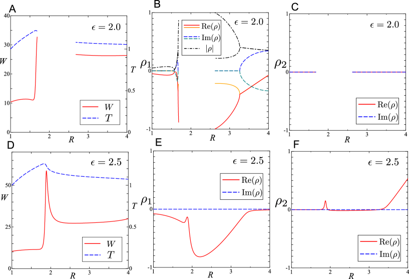
Figure 12: Entrainability $W$, period $T$, and Floquet multipliers $\rho_{i}$, as a function of $R$ for the relaxation oscillator. (A–C) $R$ dependence of (A) $W$ and $T$, (B) $\rho_{1}$, and (C) $\rho_{2}$ for $\epsilon=2.0$. (D–F) $R$ dependence of (D) $W$ and $T$, (E) $\rho_{1}$, and (F) $\rho_{2}$ for $\epsilon=2.5$. The meanings of lines are the same as in Figure 10.

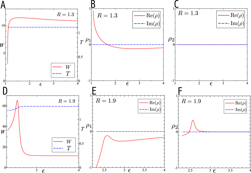
Figure 13: Entrainability $W$, period $T$, and Floquet multipliers $\rho_{i}$, as a function of $\epsilon$ for the relaxation oscillator. (A–C) $\epsilon$ dependence of (A) $W$ and $T$, (B) $\rho_{1}$, and (C) $\rho_{2}$, for $R=1.3$. (D–F) $\epsilon$ dependence of (D) $W$ and $T$, (E) $\rho_{1}$, and (F) $\rho_{2}$, for $R=1.9$. The meanings of the lines are the same as in Figure 10.

We next apply the same analysis to the relaxation oscillator: we calculated the entrainability $W$, the period $T$, and the Floquet multipliers $\rho_{i}$, as functions of $R$ (Figure 12) and $\epsilon$ (Figure 13). Figure 12A shows a dual-axis plot of the entrainability $W$ and the period $T$, for $\epsilon=2.0$ (see also Figure 10). The coupled oscillator is not $1:1$ synchronized in the region $1.7<R<2.7$, and these unsynchronized regions were not plotted. Since the entrainability $W$ grows rapidly in the vicinity of the bifurcation points ($R\simeq 1.7$) in Figure 12A, we calculated the first $\rho_{1}$ and second $\rho_{2}$ dominant Floquet multipliers in Figure 12B and C, where $\rho_{1}$ is a complex-conjugate multiplier around $R=1.7$ and is a pure real multiplier very near the bifurcation points. We see that $\rho_{1}$ of $\epsilon=2.0$ exhibits a sudden decrease towards $-1$ near $R\simeq 1.7$ and $R\simeq 2.7$, indicating that the coupled oscillator is close to the period-doubling bifurcation points. The bifurcation diagram of Figure 6 shows a branch, i.e., the period-doubling bifurcation. $\rho_{1}$ is a real multiplier for $R<3.3$, and its value approaches $-1$ as $R$ decreases toward $R=2.7$ in the vicinity of the period-doubling bifurcation. At $R\simeq 3.3$, complex-conjugate multipliers emerge instead of the annihilation of two real multipliers. Figure 12C describes the second dominant Floquet multiplier $\rho_{2}$ of $\epsilon=2.0$, and both the imaginary and real parts of $\rho_{2}$ vanish for a range of $R$ values. Because the rest of the Floquet multipliers for $\epsilon=2.0$ vanish (not shown here), all the dominant Floquet multipliers of $\epsilon=2.0$ are related to the period-doubling bifurcation points.

Figure 12D shows the entrainability $W$ and the period $T$ for $\epsilon=2.5$. We also see the rapid increase in $W$ around $R\simeq 1.9$, and the period $T$ increases up to $T=1.3$ for $1\leq R<1.9$ and then decreases for $R>1.9$. Figures 12E and F show the first $\rho_{1}$ and the second $\rho_{2}$ dominant Floquet multipliers for $\epsilon=2.5$, respectively. $\rho_{1}$ is a pure real multiplier with a minimum around $R\simeq 2.2$, which does not coincide with the position of the maximum of $W$. Although the magnitude of $\rho_{2}$ is smaller than $\rho_{1}$, it gains a peak at $R\simeq 1.9$ identical to the peak position of $W$. Thus, the system is better entrained in the vicinity of the saddle-node bifurcation, and there exists an optimal coupling strength for the entrainability.

We next show the entrainability $W$, the period $T$, and the Floquet multipliers $\rho_{i}$ as a function of $\epsilon$ for the relaxation oscillator. Figure 13A is a dual-axis plot of the entrainability $W$ and the period $T$ for $R=1.3$. We see very little dependence of the entrainability or the period on $\epsilon$. Figures 13B and C show the first $\rho_{1}$ and the second $\rho_{2}$ dominant Floquet multipliers, respectively; $\rho_{1}$ approaches $1$ with decreasing $\epsilon$, indicating that the oscillator approaches the saddle-node bifurcation points, whereas $\rho_{2}$ vanishes for a range of values of $\epsilon$. Figure 13D shows the entrainability $W$ and the period $T$ as a function of $\epsilon$ for $R=1.9$, where the period $T$ does not strongly depend on the coupling strength $\epsilon$. In contrast, the entrainability $W$ exhibits nonmonotonic behavior and achieves the local maximum around $\epsilon=2.5$. The first dominant Floquet multiplier $\rho_{1}$ in Figure 13E shows that the oscillator approaches the period-doubling bifurcation when approaching $\epsilon=2.3$ from above. Although the first dominant Floquet multiplier shows the period-doubling bifurcation, its magnitude does not qualitatively explain the existence of the entrainability peak around $\epsilon=2.5$. In contrast, the second dominant Floquet multiplier $\rho_{2}$ in Figure 13F shows a positive-valued peak around $\epsilon=2.5$, and the position agrees with that of the entrainability. In Figure 13D, enhancement is only observed inside a narrow region where $\epsilon<2.8$.

IV Discussion

Mismatched periods enhance entrainability for both smooth and relaxation oscillators, and the enhancement is related to the dominant Floquet multipliers. The behavior as a function of the model parameters ($R$ and $\epsilon$) can be explained qualitatively by a pure real Floquet multiplier. It has been previously shown that in the vicinity of the bifurcation points, the oscillator is more sensitive to an external signal Wiesenfeld:1985:PDBifAmp ; Wiesenfeld:1986:SignalAmpBif . Entrainability is thus enhanced because the period-mismatch drives the coupled oscillator to the vicinity of saddle-node bifurcation. The pure real multiplier has a strong impact on the entrainment property (Figures 10, 11, 12D–F and 13D–F), as do the Floquet multipliers related to other bifurcation types (Figures 12A–C). In Figure 12A, we see that even when neither the first nor the second dominant Floquet multiplier is a positive real multiplier, enhancement is induced by the period-doubling bifurcation points.

From our analysis above, we saw that bifurcation is less likely to occur in a smooth oscillator than in a relaxation oscillator. Nevertheless, the enhancement of entrainability (an acute peak for a relaxation oscillator and an obtuse peak for a smooth oscillator) is seen in a wider region for a smooth oscillator than for a relaxation oscillator (Figures 10A and 12D for $R$ dependence, and Figures 11A and 13D for $\epsilon$ dependence). Although a smooth oscillator may be better entrained, Figures 8 and 9 show that the amplitude of the oscillation is more strongly affected in the smooth oscillator. When increasing the period mismatch $R$, the amplitude of $y_{1}$ increases at the outset and then starts to decrease; the decrease starts sooner for the smooth oscillator than it does for the relaxation oscillator (see Figure 4 and 6). Since limit-cycle oscillations with smaller amplitude are more sensitive to external stimuli, the reduction of the amplitude that is induced by the period mismatch is also a cause of the improved entrainability. However, the main contributing factor to the enhancement is the bifurcation on the limit cycle. This is because the behavior of the entrainability $W$ agreed with that of the Floquet multiplier, which does not depend on the scaling of the values.

As mentioned in the introduction, many circadian oscillators consist of multioscillatory networks, each of which has different components. As an example, early works on Gonyaulax reported periodic bioluminescence ($24$ h to $27$ h: average $25$ h) and aggregation ($15$ h to $23$ h: average $20$ h) patterns Roenneberg:1993:TwoOsc ; Morse:1994:TwoCircadian . These two oscillators are synchronized in the presence of white light, whereas they are decoupled in the presence of dim red light. The ratio of the two periods is about $1.25$ (see Figure 2(c) in Roenneberg Roenneberg:1993:TwoOsc ), which coincides with our results of $R\simeq 1.4$ for enhancement in the smooth oscillator (see Figure 10A).

We have shown that the oscillators are better synchronized to an external signal when they are close to bifurcation points (mainly at the saddle-node but also partially at the period-doubling bifurcations). Regarding the period-doubling bifurcation in realistic systems, we note that experimental results showed the existence of a circabidian rhythm, with a 48 h period (double the circadian period). It has been reported that such circabidian rhythms can occasionally emerge under controlled conditions Honma:1988:Circabidian . The bidian rhythm may result from a period-doubling bifurcation of a circadian rhythm that is close to a bifurcation point.

Regarding stochasticity, gene expression is subject to two type of noise (stochasticity): one from the discrete molecular species (intrinsic noise) and the other from environmental variability (extrinsic noise) Koern:2005:GeneNoiseReview ; Patnaik:2006:NoiseReview ; Maheshri:2007:LivingNoisyGene ; Rausenberger:2009:GeneNoiseReview . We may take into account stochastic effects in order to make our findings biochemically realistic. For example, a collection of identical oscillators may exhibit damped oscillation as the averaging effect of stochasticity Diambra:2012:DrosphilaClock . Nevertheless, we employed a deterministic model (i.e., ordinary differential equations) in our analysis for two reasons. First, detailed stochastic modeling, such as a continuous-time discrete Markov chain, is not tractable: the only solution is an exhaustive, time-consuming calculation using the Monte Carlo method without any theoretical guarantees. Second, without analytical calculations, the theoretical arguments for the enhancement would be difficult. The enhancement we detected at the bifurcation on the limit cycle (the saddle node bifurcation) is unlikely to be found by numerical simulations, but can be deduced from Floquet multipliers. Although our present analyses do not incorporate stochastic aspects, we consider that our results help in the understanding of the stochastic dynamics in modeling mismatched periods. We will consider such stochasticity in a future study.

Another topic yet to be investigated is when three or more oscillators have mismatched periods. When considering more than two oscillators, besides the oscillatory model, the topology of the coupling is important. We can make an educated guess at the consequences of a period mismatch in such a multioscillator model: if period inconsistency drives the coupled system to the vicinity of bifurcation on the limit cycle, the period mismatch will enhances entrainability. As long as the overall connection of the multiple oscillators can be simplified as “two mismatched oscillators”, the entrainability of such a component is expected to be enhanced.

In summary, we have used phase reduction and Floquet multipliers to show that entrainability is enhanced by mismatched periods in both smooth and relaxation oscillators. We focused on two identical oscillators that were symmetrically coupled to each other by using a deterministic approach. In order to make our results more useful for real biological systems, however, it would be important to consider situations of three or more oscillators, asymmetric coupling, or structurally heterogeneous cases with stochasticity. These extensions are left to our future studies.

References

- (1) B. Novák and J. J. Tyson. Design principles of biochemical oscillators. Nat. Rev., 9:981–991, 2008.
- (2) T. Roenneberg and D. Morse. Two circadian oscillators in one cell. Nature, 362:362–364, 1993.
- (3) D. Morse, J. W. Hastings, and T. Roenneberg. Different phase responses of the two circadian oscillators in Gonyaulax. J. Biol. Rhythms, 9:263–274, 1994.
- (4) D. Gonze and A. Goldbeter. Entrainment versus chaos in a model for a circadian oscillator driven by light-dark cycles. J. Stat. Phys., 101:649–663, 2000.
- (5) D. Bell-Pedersen, V. M. Cassone, D. J. Earnest, S. S. Golden, P. E. Hardin, T. L. Thomas, and M. J. Zoran. Circadian rhythms from multiple oscillators: lessons from diverse organisms. Nat. Rev., 6:544–556, 2005.
- (6) B. C. Goodwin. Oscillatory behavior in enzymatic control processes. Advances in Enzyme Regulation, 3:425–437, 1965.
- (7) A. Wagner. Circuit topology and the evolution of robustness in two-gene circadian oscillators. PNAS, 102:11775–11780, 2005.
- (8) C. Trané and E. W. Jacobsen. On robustness as the rationale behind multiple feedback loops in the circadian clock. In Proceedings of Foundations of Systems Biology in Engineering, 2007.
- (9) M. Hafner, P. Sacré, L. Symul, R. Sepulchre, and H. Koeppl. Multiple feedback loops in circadian cycles: Robustness and entrainment as selection criteria. In Seventh International Workshop on Computational Systems Biology, pages 43–46, 2010.
- (10) M. H. Hastings. Circadian clockwork: two loops are better than one. Nat. Rev., 1:143–146, 2000.
- (11) R. Benzi, A. Sutera, and A. Vulpiani. The mechanism of stochastic resonance. J. Phys. A, 14:L453, 1981.
- (12) B. McNamara and K. Wiesenfeld. Theory of stochastic resonance. Phys. Rev. A, 39:4854–4869, 1989.
- (13) P. Jung and P. Hänggi. Amplification of small signals via stochastic resonance. Phys. Rev. A, 44:8032–8042, 1991.
- (14) P. Jung, U. Behn, E. Pantazelou, and F. Moss. Collective response in globally coupled bistable systems. Phys. Rev. A, 46:R1709–R1712, 1992.
- (15) L. Gammaitoni, P. Hänggi, P. Jung, and F. Marchesoni. Stochastic resonance. Rev. Mod. Phys., 70:223–287, 1998.
- (16) M. D. McDonnell, N. G. Stocks, C. E. M. Pearce, and D. Abbott. Stochastic resonance. Cambridge University Press, 2008.
- (17) M. D. McDonnell and D. Abbott. What is stochastic resonance? definitions, misconceptions, debates, and its relevance to biology. PLoS Comput. Biol., 5:e1000348, 2009.
- (18) Y. Hasegawa and M. Arita. Escape process and stochastic resonance under noise-intensity fluctuation. Phys. Lett. A, 375:3450–3458, 2011.
- (19) R. D. Astumian and M. Bier. Fluctuation driven ratchets: molecular motors. Phys. Rev. Lett., 72:1766–1769, 1994.
- (20) R. D. Astumian. Thermodynamics and kinetics of a Brownian motor. Science, 276:917–922, 1997.
- (21) E. Frey and K. Kroy. Brownian motion: a paradigm of soft matter and biological physics. Ann. Phys., 14:20–50, 2005.
- (22) P. Hänggi and F. Marchesoni. Artificial Brownian motors: Controlling transport on the nanoscale. Rev. Mod. Phys., 81:387–442, 2009.
- (23) Y. Hasegawa and M. Arita. Fluctuating noise drives Brownian transport. J. R. Soc. Interface, 9:3554–3563, 2012.
- (24) F. Marchesoni, L. Gammaitoni, and A. R. Bulsara. Spatiotemporal stochastic resonance in a model of kink-antikink nucleation. Phys. Rev. Lett., 76:2609–2612, 1996.
- (25) H. Nakao, K. Arai, and Y. Kawamura. Noise-induced synchronization and clustering in ensembles of uncoupled limit-cycle oscillators. Phys. Rev. Lett., 98:184101, 2007.
- (26) J. Teramae and D. Tanaka. Robustness of the noise-induced phase synchronization in a general class of limit cycle oscillators. Phys. Rev. Lett., 93:204103, 2004.
- (27) C. J. Tessone, C. R. Mirasso, R. Toral, and J. D. Gunton. Diversity-induced resonance. Phys. Rev. Lett., 97:194101, 2006.
- (28) V. K. Sharma. Adaptive significance of circadian clocks. Chronobiol. Int., 20:901–919, 2003.
- (29) L. M. Beaver, B. O. Gvakharia, T. S. Vollintine, D. M. Hege, R. Stanewsky, and J. M. Giebultowicz. Loss of circadian clock function decreases reproductive fitness in males of Drosophila melanogaster. PNAS, 19:2134–2139, 2002.
- (30) A. N. Dodd, N. Salathia, A. Hall, E. Kévei, R. Tóth, F. Nagy, J. M. Hibberd, A. J. Millar, and A. A. R. Webb. Plant circadian clocks increase photosynthesis, growth, survival and competitive advantage. Science, 309:630–633, 2005.
- (31) M. A. Woelfle, Y. Ouyang, K. Phanvijhitsiri, and C. H. Johnson. The adaptive value of circadian clocks: an experimental assessment in cyanobacteria. Curr. Biol., 14:1481–1486, 2004.
- (32) D. Gonze, S. Bernard, C. Waltermann, A. Kramer, and H. Herzel. Spontaneous synchronization of coupled circadian oscillators. Biophys. J., 89:120–129, 2005.
- (33) A. C. Liu, D. K. Welsh, C. H. Ko, H. G. Tran, E. E. Zhang, A. A. Priest, E. D. Buhr, O. Singer, K. Meeker, I. M. Verma, F. J. Doyle III, J. S. Takahashi, and S. A. Kay. Intercellular coupling confers robustness against mutations in the SCN circadian clock network. Cell, 129:605–616, 2007.
- (34) T. Y.-C. Tsai, Y. S. Choi, W. Ma, J. R. Pomerening, C. Tang, and J. E. Ferrell Jr. Robust, tunable biological osillations from interlinked positive and negative feedback loops. Science, 321:126–129, 2008.
- (35) T. Zhou, J. Zhang, Z. Yuan, and L. Chen. Synchoronization of genetic oscillators. Chaos, 18:037126, 2008.
- (36) N. Komin, A. C. Murza, E. Hernández-García, and R. Toral. Synchronization and entrainment of coupled circadian oscillators. Interface Focus, 1:167–176, 2010.
- (37) M. B. Elowitz and S. Leibler. A synthetic oscillatory network of transcriptional regulators. Nature, 403:335–338, 2000.
- (38) R. FitzHugh. Impulses and physiological states in theoretical models of nerve membrane. Biophys. J., 1:445–466, 1961.
- (39) J. Nagumo, S. Arimoto, and S. Yoshizawa. An active pulse transmission line simulating nerve axon. Proc. IRE, 50:2061–2070, 1962.
- (40) Y. Kuramoto. Chemical Oscillations, Waves, and Turbulence. Dover publications, Mineola, New York, 2003.
- (41) E. M. Izhikevich. Dynamical Systems in Neuroscience: The Geometry of Excitability and Bursting. MIT Press, 2007.
- (42) A. Pikovsky, M. Rosenblem, and J. Kurths. Synchronization: A universal concept in nonlinear sciences. Cambridge University Press, 2001.
- (43) M. A. Schwemmer and T. Lewis. The theory of weakly coupled oscillators. In N. Schultheiss, A. Prinz, and R. Butera, editors, Phase response curves in Neuroscience: Theory, Experiment and Analysis, pages 3–31. Springer, 2012.
- (44) C. A. Klausmeier. Floquet theory: a useful tool for understanding nonequilibrium dynamics. Theor. Ecol., 1:153–161, 2008.
- (45) J. Guckenheimer and P. Holmes. Nonlinear Oscillations, Dynamical Systems, and Bifurcations of Vector Fields. Springer, 1983.
- (46) J. D. Crawford. Introduction to bifurcation theory. Rev. Mod. Phys., 63:991–1037, 1991.
- (47) K. Wiesenfeld and B. McNamara. Period-doubling systems as small-signal amplifiers. Phys. Rev. Lett., 55:13–16, 1985.
- (48) K. Wiesenfeld and B. McNamara. Small-signal amplification in bifurcating dynamical systems. Phys. Rev. A, 33:629–642, 1986.
- (49) K. Honma and S. Honma. Circabidian rhythm: its appearance and disappearance in association with a bright light pulse. Experientia, 44:981–983, 1988.
- (50) M. Kœrn, T. C. Elston, W. J. Blake, and J. J. Collins. Stochasticity in gene expression: from theories to phenotypes. Nat. Rev., 6:451–464, 2005.
- (51) P. R. Patnaik. External, extrinsic and intrinsic noise in cellular systems: analogies and implications for protein synthesis. Biotechnol. Mol. Biol. Rev., 1:121–127, 2006.
- (52) N. Maheshri and E. K. O’Shea. Living with noisy genes: How cells function reliably with inherent variability in gene expression. Annu. Rev. Biophys. Biomol. Struct., 36:413–434, 2007.
- (53) J. Rausenberger, C. Fleck, J. Timmer, and M. Kollmann. Signatures of gene expression noise in cellular systems. Prog. Biophys. Mol. Biol., 100:57–66, 2009.
- (54) L. Diambra and C. P. Malta. Modeling the emergence of circadian rhythms in a clock neuron network. PLoS One, 7:e33912, 2012.