Photon Production from a Quark-Gluon-Plasma at Finite Baryon Chemical Potential

Abstract

We compute the photon production of a QCD plasma at leading order in the strong coupling with a finite baryon chemical potential. Our approach starts from the real time formalism of finite temperature field theory. We identify the class of diagrams contributing at leading order when a finite chemical potential is added and resum them to perform a full treatment of the Landau-Pomeranchuk-Migdal (LPM) effect similar to the one performed by Arnold, Moore, and Yaffe at zero chemical potential. Our results show that the contribution of $2\mapsto 3$ and $3\mapsto 2$ processes grows as the chemical potential grows.

I Introduction

Heavy ion collision experiments at RHIC typically create a medium where the net baryon density is non-vanishing Andronic et al. (2006); Braun-Munzinger and Stachel (2011). As we enter a new era of precision measurements, it is therefore important to consider the effect of a non-vanishing baryon chemical potential on the thermal photon yield of the quark gluon plasma. Previously, the effect of non-zero chemical potential in $2\leftrightarrow 2$ processes was studied in Dumitru et al. (1993); Traxler et al. (1995); Dutta et al. (2000); He et al. (2005). The complete leading order calculation of photon production including the effect of collinear enhancement in the $2\to 3$ and $3\to 2$ cases was first carried out by Arnold, Moore, and Yaffe (AMY) starting from first principles within the framework of quantum field theory at finite temperature Arnold et al. (2001a). The analysis of Arnold et al. (2001a), however, is mostly carried out at zero chemical potential. The effect of adding a chemical potential was mentioned, but a detailed analysis was not fully performed.

The chemical potential will modify the quark and gluon self-energies as well as change the statistical factors, thereby potentially modifying the power counting analysis of AMY. In this paper, we will precisely determine under which circumstances the power counting must be modified to account for the presence of a chemical potential. We also explore numerically the consequences of including a chemical potential in the photon production.

As in the previous cases, the most convenient basis to work in when analyzing the parametric sizes of diagrams is the Keldysh or $r,a$ basis whereas the rates are most conveniently written in the usual $1,2$ basis. The addition of a finite chemical potential also changes the way in which we switch from the $1,2$ basis to the $r,a$ basis, and we will carefully explain the required changes.

The organization of this paper is as follows. In section II.1, we briefly recall the structure of perturbation theory in the real time formalism and outline the basic formula giving photon production in terms of Feynman diagrams. In section II.2, we show how to generalize a result of Heinz and Wang Wang and Heinz (2002) that allows one to express Green functions in the $1,2$ basis in terms of a reduced set of Green functions in the $r,a$ basis. In section II.3, we show how a finite chemical potential alters quark and gluon thermal masses. Then, in section III, we perform a power counting analysis to determine which diagrams contribute at leading order in the strong coupling $g$ and resum these in section IV. Finally, some numerical results are shown in section V.

II Diagrammatic Approach to Calculating Photon Production

II.1 Perturbation Theory at Finite Temperature and Chemical Potential

We start by briefly outlining the structure of real time perturbation theory at finite chemical potential. Since we are interested in a QCD plasma, our starting point is the QCD Lagrangian:

$$\mathcal{L} =\sum_{f}\bar{\psi}_{f}(\not{\partial}-M-g\not{A}_{a}T^{a})\psi_{f}-\frac{1}{4}F_{\mu\nu}^{a}F_{a}^{\mu\nu}$$ (II.1)

where the sum is over the $N_{f}$ fermion flavors and the gauge group is $\mathrm{SU}(N_{c})$ with $N_{c}=3$. This Lagrangian has a conserved charge $\hat{Q}\equiv\sum_{f}\int d^{3}x\psi^{\dagger}_{f}(x)\psi_{f}(x)$ which is equal to the net fermion (quark) number. The density operator describing the grand-canonical ensemble is therefore $e^{-\beta(\hat{H}-\mu\hat{Q})}$. In the imaginary time formalism, one can show that this changes the Matsubara frequencies from $i\omega_{n}$ to $i\omega_{n}+\mu$ Kapusta and Gale (2006); Bellac (2000). The chemical potential here is hence the quark chemical potential which is 1/3 of the baryon chemical potential.

To connect the imaginary and real time formalisms, one defines the retarded and advanced propagators:

$$G_{\mathrm{Ret}}(x) =i\theta(t)\langle\{\psi(x),\bar{\psi}(0)\}\rangle_{\beta,\mu}$$ (II.2)

$$G_{\mathrm{Adv}}(x) =-i\theta(-t)\langle\{\psi(x),\bar{\psi}(0)\}\rangle_{\beta,\mu}$$ (II.3)

The anticommutators above are replaced with commutators for gauge fields. By using the spectral representation of imaginary time propagators (for instance, see Kapusta and Gale (2006); Bellac (2000)) one can show that the retarded propagator is obtained by analytically continuing the Matsubara propagator through the prescription $i\omega_{n}+\mu\mapsto p^{0}+i\epsilon$ and the advanced propagator from the continuation $i\omega_{n}+\mu\mapsto p^{0}-i\epsilon$, where $p^{0}$ is an arbitrary real number.

In the real time formalism, one is forced to double the degrees of freedom because when constructing a generating functional from the partition function, the time integration contour has to traverse the real time axis once forward and backwards (Schwinger-Keldysh Closed Time Path) Keldysh (1964). The first set of fields $\psi_{1}$, $\bar{\psi}_{1}$, and $A^{a,\mu}_{1}$ corresponds to fields with a time argument on the forward directed part of the contour and conversely the set of fields $\psi_{2}$, $\bar{\psi}_{2}$, and $A^{a,\mu}_{2}$ corresponds to fields with time arguments on the backwards directed part.

For computational purposes, it is sometimes more convenient to use another basis than the $1,2$ basis above. One such basis is the $r,a$ or Keldysh basis Keldysh (1964); Chou et al. (1985), defined as follows:

$$\varphi_{r}=\frac{\varphi_{1}+\varphi_{2}}{2}$$ (II.4)

$$\varphi_{a}=\varphi_{1}-\varphi_{2}$$ (II.5)

where $\varphi$ denotes any of our fields. By using the above algebraic relation and the spectral representation of propagators in the $r,a$ basis, one can show that for fermions:

$$G_{rr}(P) =\left(\frac{1}{2}-n_{f}(p^{0}-\mu)\right)\rho(P)$$ (II.6)

$$G_{ar}(P) =G_{\mathrm{Adv}}(P)$$ (II.7)

$$G_{ra}(P) =G_{\mathrm{Ret}}(P)$$ (II.8)

$$G_{aa}(P) =0$$ (II.9)

The above allows us to compute real time propagators by analytically continuing imaginary time ones. From now on, we use capital letters for 4-momenta and lower case letters to denote the magnitude of the 3-momenta. For instance, $P=(p^{0},{\bf p})$ in the above expressions and $p=|{\bf p}|$.

To tie this formalism to the problem of photon production, we recall the standard formula that relates the emissivity of the plasma to a Wightman current-current correlator Kapusta and Gale (2006); Bellac (2000)

$$\frac{d\Gamma_{\gamma}}{dV}=\frac{d^{3}\mathbf{k}}{(2\pi)^{3}2|\mathbf{k}|}\sum_{a=1,2}\epsilon_{\mu}^{(a)}(K)\epsilon_{\nu}^{(a)}(K)W^{\mu\nu}(K)$$ (II.10)

where we have defined the Wightman current-current correlator by:

$$W^{\mu\nu}(K)=\int d^{4}x\;e^{iK\cdot x}\langle j^{\mu}(0)j^{\nu}(x)\rangle_{\beta,\mu}$$ (II.11)

Wightman functions are most naturally expressed in the $1,2$ formalism of the real time theory:

$$d\Gamma_{\gamma} =\frac{\alpha_{EM}}{\pi^{2}}\frac{d^{3}\mathbf{k}}{|\mathbf{k}|}\int\frac{d^{4}P_{1}}{(2\pi)^{4}}\int\frac{d^{4}P_{2}}{(2\pi)^{4}}\frac{((p_{1\parallel}+k)^{2}+p_{1\parallel}^{2})}{2p_{1\parallel}(p_{1\parallel}+k)}(P_{1\perp}\cdot P_{2\perp})\times$$

$$\quad\times G_{1122}(-P_{1},K+P_{1},-K-P_{2},P_{2})$$ (II.12)

where $G_{1122}$ is a fermionic four-point function where two external vertices are of the ‘1’ types and the others are of the ‘2’ types. The “parallel” component of $\mathbf{p}$ is always defined relative to the fixed direction of the emitted photon momentum $\mathbf{k}$.

A schematic diagram for $d\Gamma_{\gamma}$ is shown in figure 1. Our convention is that fermion momenta flow into the shaded box. Arrows going into the shaded box correspond to insertions of the particle operator $\psi$, and arrows coming out of it correspond to antiparticle insertions $\bar{\psi}$.

Figure 1: The momentum assignments for computing the Wightman function. Arrows on fermion lines going into the shaded box correspond to insertions of the particle operator and those coming out of it corrrespond to insertions of the antiparticle operator. All momenta flow into the shaded box.

II.2 Going from the $1,2$ to the $r,a$ Basis

For power counting and actual computations, the $r,a$ basis is more convenient than the $1,2$ basis. By using the algebraic relation between fields in the $1,2$ and $r,a$ bases (c.f. Eq.(II.4)), we can express $G_{1122}$ as a linear combination of the sixteen possible four-point functions in the $r,a$ basis. The result is:

$$G_{1122} =G_{rrrr}+\frac{1}{2}G_{rarr}+\frac{1}{2}G_{arrr}+\frac{1}{4}G_{aarr}$$

$$-\frac{1}{2}G_{rrar}-\frac{1}{2}G_{rrra}+\frac{1}{4}G_{rraa}-\frac{1}{4}G_{rara}$$

$$-\frac{1}{4}G_{arra}-\frac{1}{4}G_{raar}-\frac{1}{4}G_{arar}+\frac{1}{8}G_{araa}$$

$$-\frac{1}{8}G_{aara}+\frac{1}{8}G_{raaa}-\frac{1}{8}G_{aaar}+\frac{1}{16}G_{aaaa}$$ (II.13)

One can show that in general, $G_{aa...a}(1,2,...,n)=0$, and hence we can immediately eliminate one of the sixteen terms in the above – See for example Chou et al. (1985). In Ref.Wang and Heinz (2002), Wang and Heinz showed that the remaining 15 terms can be re-expressed in terms of seven four-point functions and their complex conjugates.

The authors of Ref.Wang and Heinz (2002) only considered the case of a real scalar field. However, their derivation works equally well for fermions – See appendix A. Hence the following results from the reference still holds

$$G_{1122} =\alpha_{1}G_{aarr}+\alpha_{2}G_{aaar}+\alpha_{3}G_{aara}+\alpha_{4}G_{araa}+\alpha_{5}G_{raaa}+\alpha_{6}G_{arra}+\alpha_{7}G_{arar}$$

$$+\beta_{1}\bar{G}^{*}_{aarr}+\beta_{2}\bar{G}^{*}_{aaar}+\beta_{3}\bar{G}^{*}_{aara}+\beta_{4}\bar{G}^{*}_{araa}+\beta_{5}\bar{G}^{*}_{raaa}+\beta_{6}\bar{G}^{*}_{arra}+\beta_{7}\bar{G}^{*}_{arar}$$ (II.14)

with the coefficients $\alpha_{i}$ and $\beta_{i}$ composed of Fermi-Dirac distribution functions instead of Bose-Einstein distribution functions and $\bar{G}$ denoting the charge conjugate ($\bar{\psi}\leftrightarrow\psi$) of $G$. Here all $G_{\cdots}(Q_{1},Q_{2},Q_{3},Q_{4})$ are functions of 4 momenta. Our convention is that the momenta $Q_{2}$ and $Q_{4}$ correspond to the insertion of $\psi$ and $Q_{1}$ and $Q_{3}$ correspond to the insertion of $\bar{\psi}$.

This expression greatly reduces the number of diagrams we need to estimate. As a matter of fact, what emerges from our power counting analysis is that only $G_{aarr}$ contributes to photon production at leading order. This is because only this labeling gives rise to pinching poles as we will explain shortly. Thus, we only need to know the coefficients $\alpha_{1}$ and $\beta_{1}$. These are given by

$$\alpha_{1} =n_{f}(q_{1}^{0}+\mu)n_{f}(q_{2}^{0}-\mu)$$ (II.15)

$$\beta_{1} =-(1-n_{f}(q_{3}^{0}+\mu))(1-n_{f}(q_{4}^{0}-\mu))\frac{1-n_{f}(q_{1}^{0}+\mu)-n_{f}(q_{2}^{0}-\mu)}{1-n_{f}(q_{3}^{0}+\mu)-n_{f}(q_{4}^{0}-\mu)}$$ (II.16)

This is proven in Appendix A. One can intuitively understand the signs of $\mu$ in the above by recalling that $n_{f}(E-\mu)$ is the distribution function for particles while $n_{f}(E+\mu)$ is the distribution function for antiparticles. Since $Q_{1}$ and $Q_{3}$ correspond to antiparticle insertions, they must be associated with the distribution $n_{f}(q_{i}^{0}+\mu)$, and conversely for $Q_{2}$ and $Q_{4}$.

As we will discuss in section III, all gluon exchange momenta must be soft at leading order in the strong coupling $g$. Therefore, we have that $P_{1}\simeq P_{2}$ in figure 1. Hence, $Q_{1}\simeq-Q_{4}$ and $Q_{2}\simeq-Q_{3}$ and consequently, $\beta_{1}\simeq n_{f}(q_{1}^{0}+\mu)n_{f}(q_{2}^{0}-\mu)=\alpha_{1}$. Further, one can verify that $\bar{G}_{aarr}(-P_{1},K+P_{1},-K-P_{2},P_{2})=G_{aarr}(-P_{1},K+P_{1},-K-P_{2},P_{2})$ –See appendix B. Therefore, only the real part of $G_{aarr}$ is relevant to photon production at leading order.

II.3 Self-Energies at Finite Chemical Potentials

When we compute the Wightman correlator to derive the photon production, we need to do a power counting analysis to identify all leading order diagrams. In this analysis, the appearance of “pinching poles” makes it crucial to resum the thermal self-energies into the quark and gluon propagators. Therefore, we need to know how the presence of a chemical potential affects the self-energies of quarks and gluons. This is well-known and dates back to the original paper by Braaten and Pisarski on hard thermal loops Braaten and Pisarski (1990).

In order to keep our work self-contained, we review the derivation of self-energies with a full inclusion of a chemical potential in appendix C. In this section, we simply quote the final results.

The gluon polarization tensor at finite chemical potential $\mu$ takes the form:

$$\Pi_{\mu\nu}(P) =m_{D}^{2}\left(-\delta_{0}^{\mu}\delta_{0}^{\nu}+\int\frac{d\Omega}{4\pi}\frac{p^{0}v_{\mu}v_{\nu}}{p^{0}-\mathbf{v}\cdot\mathbf{p}+i\epsilon}\right)$$ (II.17)

where in the above, $m_{D}^{2}=g^{2}\left(\frac{N_{f}T^{2}}{6}+\frac{N_{c}T^{2}}{3}+\frac{N_{f}\mu^{2}}{2\pi^{2}}\right)$ is the Debye mass, and $v_{\mu}=(1,\mathbf{v})$ with $\mathbf{v}=\mathbf{k}/|\mathbf{k}|$.

Similarly, the quark self-energy at finite chemical potential is:

$$\Sigma_{T}(P) =\frac{g^{2}C_{2}(F)}{8}\left(T^{2}+\frac{\mu^{2}}{\pi^{2}}\right)\int\frac{d\Omega}{4\pi}\frac{\not{v}}{p^{0}-\mathbf{v}\cdot\mathbf{p}+i\epsilon}$$ (II.18)

The above two results show that the only effect of the chemical potential is to shift the dependence of self-energies on $T^{2}$ by a $\mu^{2}$ term. As we will see, the consequence of this is that in carrying out our power counting analysis, we need not alter the arguments of Arnold, Moore, and Yaffe as long as $\mu\leq O(T)$.

III Power Counting with a Finite Chemical Potential

When evaluating the Wightman function, there are two regions of the spatial part of the loop momentum integration that are of interest.

• The non-collinear region: ${\bf p}_{1,\perp}$ and ${\bf p}_{2,\perp}$ are both $O(T)$.

• The near-collinear region: ${\bf p}_{1,\perp}$ or ${\bf p}_{2,\perp}$ is $O(gT)$ or less.

The non-collinear region corresponds to the contributions of the basic $2\mapsto 2$ processes treated by Kapusta et al. Kapusta et al. (1991) and Baier et al. Baier et al. (1992). The near-collinear region will have both pinching pole and near-collinear enhancements. It corresponds to the contribution of the bremsstrahlung and inelastic pair annihilation processes modified by the Landau-Pomeranchuk-Migdal (LPM) effect.

We briefly review how pinching pole enhancements arise. As will be shortly shown, the leading order diagrams for photon radiation all contain a pair of fermionic propagators as shown in figure 2. The spatial part $\mathbf{p}$ of the loop momentum $P$ is assumed to be nearly collinear with $\mathbf{k}$. In other words, $\mathbf{p}_{\perp}\sim gT$.

Figure 2: The pair of fermionic propagators carry momenta which differ by $K$. We assume that $K$ is nearly collinear with $P$ and that the other parts of the diagram are essentially constant over the region of width $g^{2}T$ centered around the pinching poles of the integrand.

Given that we impose the collinearity of $\mathbf{p}$ and $\mathbf{k}$, we may focus just on the frequency integral

$$\int\frac{dp^{0}}{2\pi}G_{\mathrm{Adv}}(K+P)G_{\mathrm{Ret}}(P)=$$

$$\quad\int\frac{dp^{0}}{2\pi}\frac{1}{\left[\left(p^{0}+\frac{i\Gamma_{\mathbf{p}}}{2}\right)^{2}-E_{\mathbf{p}}^{2}\right]\left[\left(p^{0}+k^{0}-\frac{i\Gamma_{\mathbf{p}+\mathbf{k}}}{2}\right)^{2}-E_{\mathbf{p}+\mathbf{k}}^{2}\right]}$$ (III.1)

where we have absorbed the Dirac matrix structures into the vertices. In Eq.(III.1), $\Gamma_{\mathbf{p}}=\mathrm{Im}(\Sigma(P))/(2E_{\mathbf{p}})$ is the decay width of the quark generated by the imaginary part of the self energy. To leading order in $g$, it can be replaced by its asymptotic value $\Gamma=\mathrm{lim}_{\mathbf{p}\rightarrow\infty}(\Gamma_{\mathbf{p}})$ (Flechsig and Rebhan (1996); Kraemmer et al. (1990)).

The poles of the integrand are at the following locations: $p^{0}=\pm E_{\mathbf{p}}-\frac{i}{2}\Gamma$ and $p^{0}=-k^{0}\pm E_{\mathbf{p}+\mathbf{k}}+\frac{i}{2}\Gamma$. It is straightforward to see that $E_{\bf p+k}\approx p_{\parallel}+k$ when $\mathbf{p},\mathbf{k}$ are $O(T)$ and collinear. Hence the two pole positions $p^{0}=E_{p}-i\Gamma/2$ and $p^{0}=-k^{0}+E_{\bf p+k}+i\Gamma/2$ almost coincide at $p_{\parallel}\equiv\mathbf{p}\cdot\hat{k}$ although they are located on opposite halves of the contour (c.f. figure 3).

Figure 3: The locations of the four poles of the frequency integrand when $\mathbf{p}$ and $\mathbf{k}$ are nearly aligned. The poles above the real line belong to $G_{\rm adv}(K+P)$ and the ones below belong to $G_{\rm ret}(P)$. The integration contour is along the real axis. We see that two of the poles nearly coincide at $p_{\parallel}$. These poles are said to “pinch” the integration contour.

We use the residue theorem to close the contour and pick up the contributions of the poles located below the real axis. For the case where $p_{\parallel}>0$, this gives:

$$\int\frac{dp^{0}}{2\pi}G_{\mathrm{Adv}}(K+P)G_{\mathrm{Ret}}(P) \simeq\frac{-i}{2E_{\mathbf{p}}(k+E_{\mathbf{p}}-E_{\mathbf{p}+\mathbf{k}}-i\Gamma)(k+E_{\mathbf{p}}+E_{\mathbf{p}+\mathbf{k}}-i\Gamma)}$$ (III.2)

When $p_{\parallel}<0$, the factors in the denominators should be replaced by the general expression

$$E_{\mathbf{p}}-E_{\mathbf{p}+\mathbf{k}}+k \to E_{\mathbf{p}}\operatorname{sign}(p_{\parallel})-E_{\mathbf{p}+\mathbf{k}}\operatorname{sign}(p_{\parallel}+k)+k=\delta E$$ (III.3)

$$E_{\mathbf{p}}+E_{\mathbf{p}+\mathbf{k}}+k-i\Gamma \to E_{\mathbf{p}}\operatorname{sign}(p_{\parallel})+E_{\mathbf{p}+\mathbf{k}}\operatorname{sign}(p_{\parallel}+k)+k\simeq 2(p_{\parallel}+k)$$ (III.4)

Therefore, the frequency integral is approximately:

$$\int\frac{dp^{0}}{2\pi}G_{\mathrm{Adv}}(K+P)G_{\mathrm{Ret}}(P)\simeq\frac{1}{4p_{\parallel}(p_{\parallel}+k)(\Gamma+i\delta E)}$$ (III.5)

But $\Gamma$ and $\delta E$ are both of order $g^{2}T$, while $\mathbf{p}$ and $\mathbf{k}$ are hard. Hence, we get a $1/g^{2}T^{3}$ enhancement from the frequency integral. These enhancements make a large class of diagrams contribute to leading order even though we would naively expect them to be subleading.

Suppose that in the above demonstration we had not taken the integrand to be the product of an advanced and a retarded propagator but rather $\int G_{\mathrm{Adv}}(P)G_{\mathrm{Adv}}(P+K)$ or $\int G_{\mathrm{Ret}}(P)G_{\mathrm{Ret}}(P+K)$. Then all poles would have been on one side of the frequency integration contour only and we could have closed it on the side with no poles. Since the contribution from great circles at infinity vanishes, this means that the integral would vanish. Hence pinching pole enhancements only arise when we have a retarded and an advanced propagator. This is the reason why only $G_{aarr}$ contributes to the leading order photon production. Due to the fact that there is no $aa$ propagator (c.f. Eq.(II.9)) and that an interacting vertex must contain an odd number of $a$-fields Chou et al. (1985), any other labelling leads to reduction of the number of pinching poles.

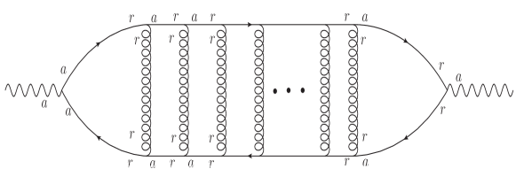
Figure 4: All ladder diagrams contribute at leading order when the gluon exchange momenta are soft.

We will illustrate general power counting arguments by estimating the size of the ladder diagram shown in figure 4. We start with the ladder diagram that has only a single rung (figure 5). Notice that the assignment of the $r,a$ indices ensures we have a retarded and an advanced propagator in each pair of quark propagators.

Figure 5: A ladder diagram with one rung only. It has two pinching pole enhancements and a further enhancement coming from the size of the soft gluon $rr$ propagator.

To get a pinching pole enhancement, we need that the quark with momentum $P$ be nearly collinear with the emitted photon. Further, if the gluon carries a soft exchange momentum $Q\sim gT$, then it cannot disturb the collinearity of the quark with the emitted photon. Therefore, the second pair of propagators also gives a pinching pole enhancement. So we have a $g^{-2}\times g^{-2}$ enhancement. A soft gluon $rr$ propagator is of order $g^{-3}T^{-2}$ because of the Bose-Einstein factor, provided $\mu\leq O(T)$. However, a soft gluon also brings in a phase space suppression of order $g^{3}$ which cancels this enhancement.

Gathering all powers, we have for suppressions:

• $g^{2}$ from the integral over $P_{\perp}$ which is $O(g^{2})$ since this is the near collinear regime.

• $g^{3}$ from the soft $Q$ spatial integral over $Q$.

• $g^{2}$ from two gluon exchange vertices.

• $g^{2}$ from the $P_{\perp}\cdot(P+Q)_{\perp}$ factor arizing from the contraction with the external photons.

and for enhancements:

• $g^{-2}\times g^{-2}$ from two pinching pole enhancements.

• $g^{-3}$ from the soft gluon propagator.

Adding up all powers of $g$, we get that this two-loop diagram is of order $g^{2}$, the same as the non-collinear one-loop diagram.

The above analysis easily extends to ladder diagrams with an arbitrary number of rungs. Each additional rung brings with it one more pinching pole enhancement, giving a $g^{-2}$, and a soft gluon propagator of order $g^{-3}$. It also brings in a $g^{3}$ suppression from the spatial integral over the new soft gluon momentum and a $g^{2}$ suppression from the two additional gauge boson exchange vertices. Adding these up, we get a net contribution of $g^{0}$, so that at least all ladder diagrams contribute to leading order.

One ought to make an important remark at this point. Since the thermal mass of the gluon goes roughly as $T^{2}+\mu^{2}/{2\pi^{2}}$, the spectral function can be of higher order than $g^{-2}$ if $\mu$ is of order $T/g$. In this case, the size of the soft $rr$ gluon propagator fails to cancel the $g^{3}$ phase space suppression that we get from a soft gluon loop momentum. Consequently, all ladder diagrams are subleading when $\mu=O(T/g)$, and it becomes unnecessary to resum the contributions of all ladder diagrams.

The rest of the power counting analysis aims at identifying which combinations of external $r,a$ indices contribute at leading order, showing that all other diagram topologies are subleading, and also proving that gauge boson momenta of order higher or less than $gT$ also give subleading contributions. As we have argued, as long as $\mu\ll T/g$, the size of the propagators comprising each diagram is parametrically the same as in the analysis of Arnold et al. (2001a). We will not pursue it here in more detail.

IV Resummation of Ladder Diagrams

In the regime where $\mu\leq O(T)$, the power counting analysis of Arnold et al. (2001a) is unchanged. Therefore, the conclusion that one needs to resum ladder diagrams (and only these) to get the photon emissivity to leading order is also valid. Hence, we can apply the same resummation procedure as Arnold et al. (2001a). Here we briefly outline that resummation procedure.

Graphically, the sum we need to evaluate is illustrated in figure 6.

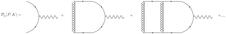
Figure 6: The resummed vertex $\mathcal{D}_{\mu}$ sums all ladder diagrams with one photon vertex removed. All external legs are amputated.

We have defined the photon resummed vertex $\mathcal{D}_{\mu}$ as the sum of all ladder diagrams with the leftmost photon vertex and pair of quark propagators removed. From figure 6, one sees that each ladder is constructed from the previous one by concatenating a gluon rung attached to two quark-gluon vertices and a pair of quark propagators to the previous one, where the quark propagators must be evaluated at the location of pinching poles. The ladder diagrams form a geometric series.

$$\mathcal{D}_{\mu}=\mathcal{I}_{\mu}+\mathcal{M}\mathcal{F}\mathcal{I}_{\mu}+\mathcal{M}\mathcal{F}\mathcal{M}\mathcal{F}\mathcal{I}_{\mu}+\mathcal{M}\mathcal{F}\mathcal{M}\mathcal{F}\mathcal{M}\mathcal{F}\mathcal{I}_{\mu}+...$$ (IV.1)

The graphical operator $\mathcal{F}$ adds the pinching pole pair of propagators. In the above equation, each ${\cal F}$ contributes a pair of pinching poles:

$$\mathcal{F}(P;K) =G_{\rm Adv}(K+P)G_{\rm Ret}(P)$$

$$\approx\frac{-1}{4p_{\parallel}(p_{\parallel}+k)}\frac{1}{\Gamma+i\delta E}4\pi\delta\left[2p^{0}+k^{0}-E_{\mathbf{p}}\operatorname{sign}(p_{\parallel})-E_{\mathbf{p}+\mathbf{k}}\operatorname{sign}(p_{\parallel}+k)\right]$$ (IV.2)

The operator $\mathcal{M}$ adds the rung as illustrated in figure 7

$$\mathcal{M}(P,Q,K)=ig^{2}C_{F}4p_{\parallel}(p_{\parallel}+k)\hat{K}_{\mu}\hat{K}_{\nu}G_{rr}^{\mu\nu}(Q)$$ (IV.3)

Figure 7: The graphical operator $\mathcal{F}$ adds a pair of propagators evaluated at the location of the pinching poles. The rung $\mathcal{M}$ adds a soft gauge boson propagator.

Finally, $\mathcal{I}_{\mu}$ is the bare photon vertex on the far end of the ladder diagram as illustrated in figure 8.

Figure 8: Bare quark-photon vertex $\mathcal{I}_{\mu}$.

The resummed vertex ${\cal D}_{\mu}$ then satisfies the following integral equation:

$$\mathcal{D}_{\mu}(P,K) =\mathcal{I}_{\mu}(P,K)+\int_{Q}\mathcal{M}(P,Q,K)\mathcal{F}(P+Q,K)\mathcal{D}_{\mu}(P+Q,K)$$ (IV.4)

After defining the variable $f^{\mu}(\mathbf{p},\mathbf{k})\equiv 4p_{\parallel}(p_{\parallel}+k)\int\frac{dp^{0}}{2\pi}\mathcal{F}(P,K)\mathcal{D}^{\mu}(P,K)$, the integral equation (IV.4) becomes Arnold et al. (2001a):

$$2P^{\mu}+K^{\mu} =i\delta Ef^{\mu}(\mathbf{p},\mathbf{k})+\int\frac{d^{3}\mathbf{q}}{(2\pi)^{3}}\mathcal{C}(\mathbf{q})\left[f^{\mu}(\mathbf{p},\mathbf{k})-f^{\mu}(\mathbf{p}+\mathbf{q}_{\perp},\mathbf{k})\right]$$ (IV.5)

After applying a sum rule, the collision kernel $\mathcal{C}(\mathbf{q})$ is found to have the simple form Aurenche et al. (2002a)

$$\int{dq_{\|}\over 2\pi}\,{\cal C}({\bf q})=\frac{1}{\mathbf{q}_{\perp}^{2}}-\frac{1}{\mathbf{q}_{\perp}^{2}+m_{D}^{2}}$$ (IV.6)

with ${\bf p}$ and ${\bf k}$ strictly colinear. The term $\delta E$ is the difference between the locations of the pinching poles of the quark propagators, as seen in Eq.(III.3). Through the energies of the quarks, it includes their asymptotic thermal masses $m_{\infty}$. Therefore, the chemical potential enters through both $m_{D}$ and $m_{\infty}$. Recall that

$$m_{D}^{2} =g^{2}\left(\frac{N_{f}T^{2}}{6}+\frac{N_{c}T^{2}}{3}+\frac{N_{f}\mu^{2}}{2\pi^{2}}\right)$$ (IV.7)

$$m_{\infty}^{2} =\frac{g^{2}C_{2}(F)}{4}\left(T^{2}+\frac{\mu^{2}}{\pi^{2}}\right)$$ (IV.8)

Finally, the contribution of the $2\mapsto 3$ and $3\mapsto 2$ processes to the Wightman correlator (and thus to the photon emissivity) is given by:

$$W_{LPM}^{\mu\nu}(K) =\int\frac{d^{4}P}{(2\pi)^{4}}\frac{(p_{\parallel}+k)^{2}+p_{\parallel}^{2}}{p_{\parallel}(p_{\parallel}+k)}\;n_{f}(p^{0}+k^{0}-\mu)[1-n_{f}(p^{0}-\mu)]\times$$

$$\quad\times\mathcal{I}^{\mu}(P,K)\mathrm{Re}[\mathcal{F}(P,K)\mathcal{D}^{\nu}(P,K)]$$ (IV.9)

V Numerical Calculations

Following a method developed by Aurenche et al. Aurenche et al. (2002b), we can solve equation (IV.4) numerically by solving the differential equation in impact parameter space. As in Ref.Arnold et al. (2001b), we decompose the photon emission rate as follows

$$(2\pi)^{3}\frac{d\Gamma}{d^{3}\mathbf{k}} ={\cal A}(k)\left[\ln(T/m_{\infty})+{1\over 2}\ln(2k/T)+C_{2\leftrightarrow 2}(k/T)+C_{\rm brem+ann}(k/T)\right]$$ (V.1)

where

$${\cal A}(k)=2\alpha_{\rm EM}\left(d_{F}\sum_{r=u,d,s}{q_{r}}^{2}\right){m_{\infty}^{2}\over k}n_{f}(k)$$ (V.2)

Here, $k$ is the magnitude of the emitted photon’s momentum and $n_{f}$ is the Fermi-Dirac factor.

Since the $2\leftrightarrow 2$ part of the spectrum has been already calculated Dumitru et al. (1993); Traxler et al. (1995); Dutta et al. (2000); He et al. (2005), we only plot $\nu_{b+a}(k)\equiv{\cal A}(k)C_{\rm brem+ann}(k/T)$ in figure 12. The plots show the contribution of the $2\mapsto 3$ and $3\mapsto 2$ processes with the full treatment of the LPM effect. The temperature of the plasma was taken to be $250\mathrm{MeV}$.

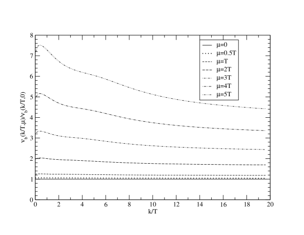
Figure 9: Combined $q$ and $\bar{q}$ bremsstrahlung contribution to the photon emission. The ratio against the $\mu=0$ case increases with increasing $\mu/T$.

Figure 10: Pair annihilation contribution. The ratio against the $\mu=0$ case decreases with increasing $\mu/T$.

We see from figure 12 that as the ratio $\mu/T$ increases, the photon production rate also increases. This finding is consistent with the behavior of the $2\leftrightarrow 2$ emission rates.

One of the reasons for this enhancement turned out to be just the statistical factors in Eq.(IV). These factors represent 3 different processes depending on the sign of $p^{0}$ and the relative sizes of $|p^{0}|$ and $k^{0}=k>0$. To illustrate the effect of non-zero $\mu$ in each of the three processes, consider the following ratio of the statistical factors in Eq.(IV) and the same statistical factors with $\mu=0$.

$$r ={n_{f}(p^{0}+k^{0}-\mu)(1-n_{f}(p^{0}-\mu))\over n_{f}(p^{0}+k^{0})(1-n_{f}(p^{0}))}$$ (V.3)

When $p^{0}>0$, the underlying physical process is the bremsstrahlung from the quarks. In this case, the ratio is mostly greater than 1. Hence the rate is enhanced. This reflects the fact that a positive chemical potential enhances the number of quarks more than the Pauli-blocking factor reduces the emission rate. When $p^{0}<0$, $(1-n_{f}(p^{0}-\mu))=n_{f}(|p^{0}|+\mu)$ becomes the anti-quark phase space density. For $p^{0}<0$ and $k<|p^{0}|$, the factor $n_{f}(-|p^{0}|+k-\mu)=1-n_{f}(|p^{0}|-k+\mu)$ represents the Pauli-blocking factor for the anti-quark bremsstrahlung. In this case, a positive chemical potential reduces the phase density of anti-quarks but enhances the Pauli-blocking factor. But since Pauli-blocking can never be enhanced above 1, the effect is to reduce the photon emission rate. The combined effect of quark bremsstrahlung and anti-quark bremsstrahlung is a net enhancement as shown in figure 9.

For $p^{0}<0$ and $k>|p^{0}|$, the factor $n_{f}(-|p^{0}|+k-\mu)$ represents the density of quarks that can annihilate with anti-quarks to produce a photon with energy $k$. In this case $r$ is always smaller than $1$, reflecting the fact that the annihilation process is necessarily controlled by the lesser number of anti-quarks. In figure 10, we show the contribution of the annihilation process to the photon emission rate for various values of $\mu$.

Among these three effects, the enhancement of the quark-bremsstrahlung dominates because it increases much faster than the reductions in the annihilation contribution and the anti-quark bremsstrahlung. Therefore, overall, the effect of having $\mu>0$ is to enhance the photon production at the same temperature as shown in figures 11 and 12. This trend was also observed in studies of $2\leftrightarrow 2$ processes Traxler et al. (1995). In one previous study of $2\leftrightarrow 2$ processes Dumitru et al. (1993), it was found that increasing the chemical potential decreases photon production. However, this was for constant energy density instead of constant temperature.

Figure 11: For $\mu$ of the order of the temperature $T$ of the plasma, the photon emission rate increases by about $10\%$ relative to the $\mu=0$ value.

Figure 12: Plots of the ratios $\nu_{b+a}(\mu)/\nu_{b+a}(\mu=0)$ for $0\leq\mu\leq 10T$. As $\mu/T$ increases, so does the ratio.

Phenomenologically, the baryon chemical potential at RHIC is about 30 MeV and at SPS it is about 240 MeVBraun-Munzinger et al. (2002). The quark chemical potential is therefore about $10\,\hbox{MeV}$ and $80\,\hbox{MeV}$ for RHIC and SPS, respectively. With $T=O(200\,\hbox{MeV})$, the enhancement at RHIC is negligibly small and it will be modest at SPS, no more than 5 %.

VI Conclusion

In this paper, we have explored the effect of non-zero baryon chemical potential in thermal photon production. Following the zero chemical potential study Arnold et al. (2001a), we have computed photon production from non-Abelian plasmas at leading order by resumming ladder diagrams to fully incorporate the LPM effect. After a careful analysis, we have found that as long as $\mu\leq O(T)$, the formulation in Arnold et al. (2001a) is still valid with appropriate changes in the statistical factors, thermal masses and the Debye mass. However, when $\mu=O(T/g)$, resummation of ladder diagrams is no longer necessary because thermal masses become $O(T)$ instead of $O(gT)$. Hence, inverse powers of thermal masses no longer provide enhancements.

Numerically, it is found that the inclusion of a chemical potential up to $\mu\simeq T$ enhances the photon emission rate moderately, up to $30\,\%$ when $\mu=T$. This trend is also valid for hard photons from the $2\leftrightarrow 2$ processTraxler et al. (1995). Since the quark chemical potential is relatively small compared to typical QGP temperatures at RHIC and the LHC, we expect a relatively small effect from a finite $\mu$ on thermal photon production at RHIC and the LHC although it could be significant at SPS energies and also for the lower energy runs at RHIC.

Appendix A KMS Condition with Finite $\mu$

In this appendix, our goal is to prove equation (II.14). This equation was proven in reference Wang and Heinz (2002) for the case of scalar fields. Their argument exploits the KMS condition to derive a system of equations that allows them to solve for $G_{rrrr}$, $G_{rrra}$, $G_{rrar}$, $G_{rarr}$, $G_{arrr}$, $G_{raar}$, $G_{rara}$, and $G_{rraa}$ in terms of $G_{aarr}$, $G_{aaar}$, $G_{aara}$, $G_{araa}$, $G_{raaa}$, $G_{arra}$, $G_{arar}$ and their complex conjugates. Their procedure also goes through for Dirac fermions in the grand canonical ensemble provided we modify the usual KMS condition to include a chemical potential.

Consider first the commutation relation between Dirac field operators and the conserved charge $\hat{Q}$:

$$[\hat{Q},\psi]=-\psi \Rightarrow e^{\beta\mu\hat{Q}}\psi=e^{-\beta\mu}\psi e^{\beta\mu\hat{Q}}$$

$$[\hat{Q},\bar{\psi}]=\bar{\psi} \Rightarrow e^{\beta\mu\hat{Q}}\bar{\psi}=e^{\beta\mu}\bar{\psi}e^{\beta\mu\hat{Q}}$$ (A.1)

For Green functions in the $1,2$ basis, these commutation relations allow us to relate Green functions whose $1,2$ index assignments are opposite each other. Indeed, consider:

$$G_{2..21..1}(x_{1},...,x_{n}) =\langle\tilde{T}(\psi^{\dagger}(x_{1})...\psi^{\dagger}(x_{r})\psi(x_{r+1})...\psi(x_{m}))\times$$

$$\quad\times T(\psi^{\dagger}(x_{m+1})...\psi^{\dagger}(x_{l})\psi(x_{l+1})...\psi(x_{n}))\rangle_{\beta,\mu}$$ (A.2)

Note that the $2$ index refers to the space-time points $x_{1},...,x_{m}$ and the $1$ index refers to the points $x_{m+1},...,x_{n}$. We have also omitted spinor indices in the above for simplicity. Using the fact that $e^{\beta\hat{H}}$ is a time evolution operator in imaginary time ($\psi(t+i\beta)=e^{-\beta\hat{H}}\psi(t)e^{\beta\hat{H}}$), we obtain:

$$G_{2..21..1}(x_{1},...,x_{n})=$$

$$\quad\langle\tilde{T}(e^{\beta\hat{H}}\psi^{\dagger}(x_{1}^{0}+i\beta)...\psi^{\dagger}(x_{r}^{0}+i\beta)\psi(x_{r+1}^{0}+i\beta)...\psi(x_{m}^{0}+i\beta)e^{-\beta\hat{H}})\times$$

$$\quad\times T(\psi^{\dagger}(x_{m+1})...\psi^{\dagger}(x_{l})\psi(x_{l+1})...\psi(x_{n}))\rangle_{\beta,\mu}$$ (A.3)

The operators $e^{\pm\beta\hat{H}}$ can be pulled outside of the reversed time-ordering symbol. Therefore, when writing out the thermal average explicitly in terms of the density operator $e^{-\beta(\hat{H}-\mu\hat{Q})}$ , we obtain:

$$G_{2..21..1}(x_{1},...,x_{n})=$$

$$\quad\frac{1}{Z}\operatorname{Tr}(e^{\beta\mu\hat{Q}}\tilde{T}(\psi^{\dagger}(x_{1}^{0}+i\beta)...\psi^{\dagger}(x_{r}^{0}+i\beta)\psi(x_{r+1}^{0}+i\beta)...\psi(x_{m}^{0}+i\beta))\times$$

$$\quad\times e^{-\beta\hat{H}}T(\psi^{\dagger}(x_{m+1})...\psi^{\dagger}(x_{l})\psi(x_{l+1})...\psi(x_{n})))$$ (A.4)

We want to commute the operators inside the reverse time-ordering operator past $e^{\beta\mu\hat{Q}}$ and use the cyclicity of the trace to take them to the right of the operators inside the time-ordering symbol. Equation (A.1) shows that in doing this, we pick up a factor of $e^{\beta\mu}$ when we are commuting a $\psi^{\dagger}$ operator and a factor of $e^{-\beta\mu}$ for a $\psi$ operator. Let us define the symbol $\sigma_{i}$ to be equal to $1$ if the space-time point $x_{i}$ has a $\psi^{\dagger}$ operator insertion at it, or $-1$ if it has a $\psi$ insertion. With this notation, we obtain the following generalization of the KMS boundary condition to $n$-point functions:

$$G_{2..21..1}(x_{1},...,x_{n})=$$

$$\quad\frac{1}{Z}e^{\sum_{i|a_{i}=2}\sigma_{i}\beta\mu}\operatorname{Tr}(e^{-\beta(\hat{H}-\mu\hat{Q})}T(\psi^{\dagger}(x_{m+1})...\psi^{\dagger}(x_{l})\psi(x_{l+1})...\psi(x_{n}))\times$$

$$\quad\times\tilde{T}(\psi^{\dagger}(x_{1}^{0}+i\beta)...\psi^{\dagger}(x_{r}^{0}+i\beta)\psi(x_{r+1}^{0}+i\beta)...\psi(x_{m}^{0}+i\beta)))$$ (A.5)

Finally, we use the well-known formula $\phi(t+a)=e^{a\partial_{t}}\phi(t)$ to obtain:

$$G_{2..21..1}(x_{1},...,x_{n})=$$

$$\quad e^{\beta\sum_{i|a_{i}=2}(i\partial_{t_{i}}+\sigma_{i}\mu)}\langle T(\psi^{\dagger}(x_{m+1})...\psi^{\dagger}(x_{l})\psi(x_{l+1})...\psi(x_{n}))\times$$

$$\quad\times\tilde{T}(\psi^{\dagger}(x_{1}^{0})...\psi^{\dagger}(x_{r}^{0})\psi(x_{r+1}^{0})...\psi(x_{m}^{0}))\rangle_{\beta,\mu}$$ (A.6)

We are allowed to take the $e^{\sum_{i|a_{i}=2}i\beta\partial_{t_{i}}}$ operator outside of the time-ordering symbol provided we take time-ordering to be given by the $T^{*}$ prescription. That is, the time-ordered $n$-point function is defined to be the path integral of the product of the $n$ operators weighted by the exponential of $i$ times the action. For a discussion of this prescription, see for example Itzykson and Zuber (1980).

We define the “tilde conjugate” $\tilde{G}$ of a Green function $G$ to have same $1,2$ index assignment but with the time-ordering symbols reversed. Therefore, we can express our previous result as:

$$G_{2..21..1}(x_{1},...,x_{n})=e^{\beta\sum_{i|a_{i}=2}(i\partial_{t_{i}}+\sigma_{i}\mu)}\tilde{G}_{1..12..2}(x_{1},...,x_{n})$$ (A.7)

In Wang and Heinz (2002), Wang and Heinz use the fact that in momentum space, tilde conjugation is equivalent to complex conjugation. As this is a key fact, we proceed to extend it to fermion fields at finite chemical potential. For notational simplicity, we will focus on the case where there are four fermion operators two of which bear “$1$” indices, and the other two of which bear “$2$” indices. Although this is not necessary for this discussion, we have also included the $\gamma$ matrices which appear in the current-current correlator II.11. Extensions to other cases should be obvious.

$$G_{2211}(Q_{1},Q_{2},Q_{3},Q_{4}) =\int\prod_{i=1}^{4}d^{4}x_{i}\;e^{iQ_{i}\cdot x_{i}}\langle\tilde{T}(\bar{\psi}(x_{1})\gamma^{\mu}\psi(x_{2}))T(\bar{\psi}(x_{3})\gamma^{\nu}\psi(x_{4}))\rangle_{\beta,\mu}$$ (A.8)

Taking a complex conjugation and changing $x_{i}\to-x_{i}$, we obtain:

$$G_{2211}^{*}(Q_{1},Q_{2},Q_{3},Q_{4}) =\int\prod_{i=1}^{4}d^{4}x_{i}\;e^{iQ_{i}\cdot x_{i}}\langle T(\bar{\psi}(-x_{4})\gamma^{\nu}\psi(-x_{3}))\tilde{T}(\bar{\psi}(-x_{2})\gamma^{\mu}\psi(-x_{1}))\rangle_{\beta,\mu}$$ (A.9)

Next, we make use of $C\!PT$ invariance. Recall that the Dirac bilinear $\bar{\psi}\gamma^{\mu}\psi$ transforms as follows under the anti-unitary $C\!PT$ transformation $\Theta$:

$$\Theta\bar{\psi}(x)\gamma^{\mu}\psi(y)\Theta^{-1} =-\bar{\psi}(-y)\gamma^{\mu}\psi(-x)$$ (A.10)

Then, using anti-unitarity, thermal expectations of a product of fields can be related as follows:

$$\langle T(\bar{\psi}(-x_{4})\gamma^{\nu}\psi(-x_{3}))\tilde{T}(\bar{\psi}(-x_{2})\gamma^{\mu}\psi(-x_{1}))\rangle_{\beta,\mu}^{*}$$

$$=\frac{1}{Z}\sum_{n}\langle n|e^{-\beta(\hat{H}-\mu\hat{Q})}T(\bar{\psi}(-x_{4})\gamma^{\nu}\psi(-x_{3}))\tilde{T}(\bar{\psi}(-x_{2})\gamma^{\mu}\psi(-x_{1}))|n\rangle^{*}$$

$$=\frac{1}{Z}\sum_{n}\langle\Theta n|\Theta e^{-\beta(\hat{H}-\mu\hat{Q})}T(\bar{\psi}(-x_{4})\gamma^{\nu}\psi(-x_{3}))\tilde{T}(\bar{\psi}(-x_{2})\gamma^{\mu}\psi(-x_{1}))\Theta^{-1}|\Theta n\rangle$$

$$=\frac{1}{Z}\sum_{n^{\prime}}\langle n^{\prime}|e^{-\beta(\hat{H}+\mu\hat{Q})}T(\Theta\bar{\psi}(-x_{4})\gamma^{\nu}\psi(-x_{3})\Theta^{-1})\tilde{T}(\Theta\bar{\psi}(-x_{2})\gamma^{\mu}\psi(-x_{1})\Theta^{-1})|n^{\prime}\rangle$$

$$=\frac{1}{Z}\sum_{n^{\prime}}\langle n^{\prime}|e^{-\beta(\hat{H}+\mu\hat{Q})}T(\bar{\psi}(x_{3})\gamma^{\nu}\psi(x_{4}))\tilde{T}(\bar{\psi}(x_{1})\gamma^{\mu}\psi(x_{2}))|n^{\prime}\rangle$$

$$=\langle T(\bar{\psi}(x_{3})\gamma^{\nu}\psi(x_{4}))\tilde{T}(\bar{\psi}(x_{1})\gamma^{\mu}\psi(x_{2}))\rangle_{\beta,-\mu}$$ (A.11)

We have used $C\!PT$ invariance in commuting $\Theta$ past $e^{-\beta\hat{H}}$ and relabeling the eigenstates $|n^{\prime}\rangle=\Theta|n\rangle$. Further, note that the sign of $\mu$ changes as we commute $\Theta$ past $e^{\beta\mu\hat{Q}}$. Combining the above with our previous result, we obtain:

$$G_{2211}^{*}(Q_{1},Q_{2},Q_{3},Q_{4}) =\int\prod_{i=1}^{4}d^{4}x_{i}\;e^{iQ_{i}\cdot x_{i}}\langle T(\bar{\psi}(-x_{4})\gamma^{\nu}\psi(-x_{3}))\tilde{T}(\bar{\psi}(-x_{2})\gamma^{\mu}\psi(-x_{1}))\rangle_{\beta,\mu}$$

$$=\int\prod_{i=1}^{4}d^{4}x_{i}\;e^{iQ_{i}\cdot x_{i}}\langle T(\bar{\psi}(x_{2})\gamma^{\mu}\psi(x_{1}))\tilde{T}(\bar{\psi}(x_{4})\gamma^{\nu}\psi(x_{3}))\rangle_{\beta,-\mu}$$

$$=\tilde{\bar{G}}_{2211}(Q_{1},Q_{2},Q_{3},Q_{4})$$ (A.12)

where $\bar{G}$ denotes the charge conjugate ($\bar{\psi}\leftrightarrow\psi$) of $G$. Recapitulating, we have the two equations:

$$G_{2..21..1}(K_{1},...,K_{n}) =e^{\beta\sum_{i|a_{i}=2}(k_{i}^{0}+\sigma_{i}\mu)}\tilde{G}_{2..21..1}^{*}(K_{1},...,K_{n})$$

$$\tilde{G}_{2..21..1}(K_{1},...,K_{n}) =\bar{G}^{*}_{2..21..1}(K_{1},...,K_{n})$$ (A.13)

The above can be taken as the starting point to reproduce the derivation of Heinz and Wang. However, the latter also uses the energy conservation condition $\sum_{i}k_{i}^{0}=0$ and the identity $n_{b}(k_{i}^{0})+n_{b}(-k_{i}^{0})=-1$. In order for the derivation of Heinz and Wang to proceed in the same manner, we need suitable generalizations of these to treat fermions at finite chemical potential. By charge conservation, we must have that $\sum_{i=1}^{n}\sigma_{i}=0$ – In other words, the Green function in question must have an equal number of $\psi^{\dagger}$ and $\psi$ insertions to not vanish. Therefore, we can define $\tilde{k}_{i}^{0}\equiv k_{i}^{0}+\sigma_{i}\mu$ and maintain “energy conservation” $\sum_{i=1}^{n}\tilde{k}_{i}^{0}=0$. Also, by performing the customary replacement $n_{b}(k_{i}^{0})\mapsto-n_{f}(\tilde{k}_{i}^{0})$, we preserve the relation $n_{b}(k_{i}^{0})+n_{b}(-k_{i}^{0})=-1$ since $n_{f}(E)+n_{f}(-E)=1$ in general.

The only relations among the $k_{i}^{0}$’s that Heinz and Wang use is energy conservation, and the only property of the Bose-Einstein distributions they use is $n_{b}(k_{i}^{0})+n_{b}(-k_{i}^{0})=-1$. This is because after they have used the KMS condition like we have done above, their work consists of algebraic manipulations such as solving large systems of equations involving the Bose-Einstein distribution. In their work, it is possible to treat $G$ and $G^{*}$ as independent variables rather than considering the real and imaginary parts of $G$. Hence, it causes no harm to their derivation to replace $G^{*}$ by $\bar{G}^{*}$ as is required by (A.13). We conclude that we could in principle perform the exact same manipulations as Heinz and Wang by relabeling every $n_{b}(k_{i}^{0})$ as $-n_{f}(\tilde{k}_{i}^{0})$. The net result is that we make the same replacements in their final results, bearing in mind that $\psi^{\dagger}$ insertions come with a $-n_{f}(k^{0}+\mu)$ and $\psi$ insertions come with $-n_{f}(k^{0}-\mu)$.

In reference Wang and Heinz (2002), Heinz and Wang obtain

$$\alpha_{1}=n_{b}(q_{1}^{0})n_{b}(q_{2}^{0})$$ (A.14)

and

$$\beta_{1}=-(1+n_{b}(q_{3}^{0}))(1+n_{b}(q_{4}^{0}))\frac{1+n_{b}(q_{1}^{0})+n_{b}(q_{2}^{0})}{1+n_{b}(q_{3}^{0})+n_{b}(q_{4}^{0})}$$ (A.15)

By making the replacements we have prescribed above, we get:

$$\alpha_{1}=n_{f}(q_{1}^{0}+\mu)n_{f}(q_{2}^{0}-\mu)$$ (A.16)

and

$$\beta_{1}=-(1-n_{f}(q_{3}^{0}+\mu))(1-n_{f}(q_{4}^{0}-\mu))\frac{1-n_{f}(q_{1}^{0}+\mu)-n_{f}(q_{2}^{0}-\mu)}{1-n_{f}(q_{3}^{0}+\mu)-n_{f}(q_{4}^{0}-\mu)}$$ (A.17)

as required.

Appendix B A Simple Identity Involving Charge Conjugates

In this appendix, we want to show that $\bar{G}_{aarr}(K_{1},K_{2},K_{3},K_{4})=G_{aarr}(K_{1},K_{2},K_{3},K_{4})$. It is sufficient to prove the corresponding identity in position space.

$$G_{aarr}(x_{1},x_{2},x_{3},x_{4}) \equiv\langle T_{C}(\bar{\psi}_{a}(x_{1})\psi_{a}(x_{2})\bar{\psi}_{r}(x_{3})\psi_{r}(x_{4}))\rangle_{\beta,\mu}$$

$$\Rightarrow\bar{G}_{aarr}(x_{1},x_{2},x_{3},x_{4}) =\langle T_{C}(\bar{\psi}_{a}(x_{2})\psi_{a}(x_{1})\bar{\psi}_{r}(x_{4})\psi_{r}(x_{3}))\rangle_{\beta,-\mu}$$

$$=\frac{1}{Z}\sum_{n}\langle n|e^{-\beta(\hat{H}+\mu\hat{Q})}T_{C}(\bar{\psi}_{a}(x_{2})\psi_{a}(x_{1})\bar{\psi}_{r}(x_{4})\psi_{r}(x_{3}))|n\rangle$$

$$=\frac{1}{Z}\sum_{n}\langle Cn|Ce^{-\beta(\hat{H}+\mu\hat{Q})}T_{C}(\bar{\psi}_{a}(x_{2})\psi_{a}(x_{1})\bar{\psi}_{r}(x_{4})\psi_{r}(x_{3}))C^{\dagger}|Cn\rangle$$

$$=\frac{1}{Z}\sum_{n^{\prime}}\langle n^{\prime}|e^{-\beta(\hat{H}-\mu\hat{Q})}CT_{C}(\bar{\psi}_{a}(x_{2})\psi_{a}(x_{1})\bar{\psi}_{r}(x_{4})\psi_{r}(x_{3}))C^{\dagger}|n^{\prime}\rangle$$

$$=\frac{1}{Z}\sum_{n^{\prime}}\langle n^{\prime}|e^{-\beta(\hat{H}-\mu\hat{Q})}T_{C}(C\bar{\psi}_{a}(x_{2})\psi_{a}(x_{1})C^{\dagger}C\bar{\psi}_{r}(x_{4})\psi_{r}(x_{3})C^{\dagger})|n^{\prime}\rangle$$

$$=\frac{1}{Z}\sum_{n^{\prime}}\langle n^{\prime}|e^{-\beta(\hat{H}-\mu\hat{Q})}T_{C}(\bar{\psi}_{a}(x_{1})\psi_{a}(x_{2})\bar{\psi}_{r}(x_{3})\psi_{r}(x_{4}))|n^{\prime}\rangle$$

$$=G_{aarr}(x_{1},x_{2},x_{3},x_{4})$$

Appendix C Computation of Self-Energies at Finite Chemical Potentials

In this appendix, we closely follow the zero $\mu$ analysis in Blaizot and Iancu (2002) to compute self-energies in the hard thermal loop approximation with a finite chemical potential.

Consider first the gluon self-energy $\Pi^{ab}_{\mu\nu}$. The color structure of this tensor is trivial, so that $\Pi_{\mu\nu}^{ab}=\delta^{ab}\Pi_{\mu\nu}$. We have four diagrams to consider: the quark loop, the gluon loop, the gluon tadpole, and the gluon ghost. Only the quark loop is affected by the presence of a chemical potential and hence we make it the focus of our attention. With all momenta labeled, this diagram is shown in figure 13.

Figure 13: The quark loop is the only contribution to the gluon self-energy that is affected by the finite chemical potential $\mu$.

Our strategy is to evaluate this diagram in the imaginary-time, invert it to get the gluon propagator, and then analytically continue the result to retarded frequencies to get the real-time $ra$ propagator from which all other propagators in the $r,a$ basis may be obtained. Proceeding, we first get:

$$\Pi_{\mu\nu}(P_{E}) =g^{2}\operatorname{Tr}(T^{a}T^{a})\int\{dK_{E}\}\ Tr(\gamma_{\mu}S_{F}^{\prime(\mu)}(K_{E})\gamma_{\nu}S_{F}^{\prime(\mu)}(Q_{E}))$$ (C.1)

In the above, the integration measure is $\{dK_{E}\}=T\sum_{r=-\infty}^{\infty}\int(d\mathbf{k})$, where $(d\mathbf{k})=\frac{d^{3}\mathbf{k}}{(2\pi)^{3}}$ is the spatial momentum integration measure. Since we have factored out the color structure of the gluon self-energy, there is no sum over $a$ in the $\operatorname{Tr}(T^{a}T^{a})$ factor. Further, $K_{E}=(i\omega_{r},\mathbf{k})$ is the fermionic loop momentum and $Q_{E}=K_{E}-P_{E}=(i\omega_{r}-i\omega_{n},\mathbf{k}-\mathbf{p})$ is the difference between the momentum of the gluon ($P_{E}=(i\omega_{n},{\bf p})$) and the virtual quark. The frequency $i\omega_{n}=2\pi nT$ is bosonic, and the frequency $i\omega_{r}=2\pi(r+\frac{1}{2})T$ is fermionic. The color matrices $T^{a}$ are the generators of $\mathrm{SU(3)}$ in the fundamental representation. In this representation, the group factor $\operatorname{Tr}(T^{a}T^{a})$ is simply $\frac{1}{2}$. $S_{F}^{\prime(\mu)}$ denotes the fermion propagator time evolved using the “thermodynamics Hamiltonian” $\hat{H}-\mu\hat{Q}$ since this is what satisfies the periodic boundary condition (see Appendix A for KMS conditions at finite $\mu$).

The cleanest way to compute the above is to use the spectral representation

$$S_{F}^{\prime(\mu)}(i\omega_{r},\mathbf{k}) =\int_{0}^{\beta}d\tau\;e^{i\omega_{r}\tau}\int_{-\infty}^{\infty}\frac{dk^{0}}{2\pi}(1-n_{f}(k^{0}-\mu))\not{K}e^{-\tau(k^{0}-\mu)}\rho_{0}(K)$$ (C.2)

Indeed, this expansion of the propagator makes the frequency sum trivial. After performing the spin trace and employing standard identities involving the Fermi-Dirac distribution, we obtain:

$$\Pi^{(a)}_{\mu\nu}(i\omega_{n},\mathbf{p}) =2g^{2}N_{f}\int(d\mathbf{k})\int\frac{dk^{0}}{2\pi}\int\frac{dq^{0}}{2\pi}\rho_{0}(K)\rho_{0}(Q)\times$$

$$\quad\times(K_{\mu}Q_{\nu}+Q_{\mu}K_{\nu}-g_{\mu\nu}K\cdot Q)\frac{n_{f}(k^{0}-\mu)-n_{f}(q^{0}-\mu)}{k^{0}-q^{0}-i\omega_{n}}$$ (C.3)

For the spatial component of the self-energy tensor, the result is

$$\Pi_{ij}(i\omega,\mathbf{p}) =2g^{2}N_{f}\int(d\mathbf{k})\frac{1}{4E_{\mathbf{k}}E_{\mathbf{q}}}\biggl{[}(k_{i}q_{j}+q_{i}k_{j}+\delta_{ij}(E_{\mathbf{k}}E_{\mathbf{q}}-\mathbf{k}\cdot\mathbf{q}))$$

$$\qquad\times\left(\frac{n_{f}(E_{\mathbf{k}}+\mu)-n_{f}(E_{\mathbf{q}}+\mu)}{i\omega+E_{\mathbf{k}}-E_{\mathbf{q}}}-\frac{n_{f}(E_{\mathbf{k}}-\mu)-n_{f}(E_{\mathbf{q}}-\mu)}{i\omega-E_{\mathbf{k}}+E_{\mathbf{q}}}\right)$$

$$\quad+(k_{i}q_{j}+q_{i}k_{j}-\delta_{ij}(E_{\mathbf{k}}E_{\mathbf{q}}+\mathbf{k}\cdot\mathbf{q}))$$

$$\qquad\times\left(\frac{1-n_{f}(E_{\mathbf{k}}+\mu)-n_{f}(E_{\mathbf{q}}-\mu)}{i\omega+E_{\mathbf{k}}+E_{\mathbf{q}}}-\frac{1-n_{f}(E_{\mathbf{q}}+\mu)-n_{f}(E_{\mathbf{k}}-\mu)}{i\omega-E_{\mathbf{k}}-E_{\mathbf{q}}}\right)\biggr{]}$$ (C.4)

using $\rho_{0}(K)=\frac{\pi}{E_{\mathbf{k}}}\left(\delta(k^{0}-k)-\delta(k^{0}+k)\right)$. The above expression holds for arbitrary external momenta. Henceforth, we only consider the hard thermal loop approximation so that $p\ll k$ after the analytic continuation $i\omega\mapsto p^{0}+i\epsilon$ has been performed. It turns out that the self-energies in the hard thermal loop approximation are also valid for arbitrary external momenta $P$ at the one loop order Flechsig and Rebhan (1996); Kraemmer et al. (1990). Hence, we will freely use our results as the self-energies of the gluons and quarks when estimating the size of their propagators.

Using the fact that $p\ll k$, we obtain:

$$\Pi_{ij}(p^{0},\mathbf{p}) =-g^{2}N_{f}\int(d\mathbf{k})\biggl{[}v_{i}v_{j}\frac{\mathbf{v}\cdot\mathbf{p}}{p^{0}-\mathbf{v}\cdot\mathbf{p}+i\epsilon}\frac{d}{dk}(n_{f}(k-\mu)+n_{f}(k+\mu))$$

$$\quad+(v_{i}v_{j}-\delta_{ij})\frac{1}{k}(n_{f}(k-\mu)+n_{f}(k+\mu))\biggr{]}$$ (C.5)

where ${\bf v}={\bf k}/|{\bf k}|$. After an integration by parts and an application of the result

$$\int_{0}^{\infty}(dk)k\left(\frac{1}{e^{\beta(k+\mu)}+1}+\frac{1}{e^{\beta(k-\mu)}+1}\right)=\frac{\pi^{2}T^{2}}{6}+\frac{\mu^{2}}{2}$$ (C.6)

we get:

$$\Pi_{ij}(p^{0},\mathbf{p}) =-g^{2}N_{f}\left(\frac{\mu^{2}}{2}+\frac{\pi^{2}T^{2}}{6}\right)\int{d\Omega\over 8\pi^{3}}\left[v_{i}v_{j}-\delta_{ij}-2(v_{i}v_{j})\frac{\mathbf{v}\cdot\mathbf{p}}{p^{0}-\mathbf{v}\cdot\mathbf{p}+i\epsilon}\right]$$ (C.7)

By symmetry, we have $\int d\Omega v_{i}v_{j}=\frac{1}{3}\int d\Omega\delta_{ij}$. Thus, we finally obtain the hard thermal loop part of the gluon polarization tensor.

$$\Pi_{ij}(P) =g^{2}N_{f}\left(\frac{\mu^{2}}{2}+\frac{\pi^{2}T^{2}}{6}\right)\int\frac{d\Omega}{4\pi^{3}}\frac{p^{0}v_{i}v_{j}}{p^{0}-\mathbf{v}\cdot\mathbf{p}+i\epsilon}$$ (C.8)

By going through the same analysis, we can evaluate the other components of the gluon polarization tensor. If we include the contributions of the three other loops, we finally have:

$$\Pi_{\mu\nu}(P) =m_{D}^{2}\left(-\delta_{0}^{\mu}\delta_{0}^{\nu}+\int\frac{d\Omega}{4\pi}\frac{p^{0}v_{\mu}v_{\nu}}{p^{0}-\mathbf{v}\cdot\mathbf{p}+i\epsilon}\right)$$ (C.9)

where in the above, $m_{D}^{2}=g^{2}\left(\frac{N_{f}T^{2}}{6}+\frac{N_{c}T^{2}}{3}+\frac{N_{f}\mu^{2}}{2\pi^{2}}\right)$ is the Debye mass, and $v_{\mu}=(1,\mathbf{v})$.

The contribution of the quark loop to the gluon self-energy corresponds to the screening of the strong interaction by quarks in the medium. It is therefore natural to expect that the chemical potential of the quarks will have an influence on the repeated scattering events that occur during the photon emission process. The chemical potential also appears explicitly in the quark propagator and thus affects the thermal mass of the quarks. This will affect the integral equation that we will derive for photon production, so we turn to computing the self-energy of the quarks. The relevant diagram is shown in figure 14.

Figure 14: The chemical potential appears explicitly in the quark propagators, whence we need to resum the self-energy of the quark.

The expression corresponding to the diagram in figure 14 is:

$$\Sigma(P_{E}) =g^{2}T^{a}T^{a}\int\{dQ_{E}\}\gamma_{\mu}S_{F}^{\prime\mu}(P_{E}-Q_{E})\gamma_{\nu}G^{\mu\nu}(Q_{E})$$ (C.10)

In the above, $\int\{dQ_{E}\}\equiv T\sum_{n=-\infty}^{\infty}\int(d\mathbf{q})$ denotes a sum over bosonic frequencies followed by an integration over the spatial part of $Q$. As usual, $T^{a}T^{a}=C_{2}(F)\mathbf{1}=\frac{4}{3}\mathbf{1}$ where $\mathbf{1}$ is the identity matrix in $\mathrm{SU(3)}$. In the Coulomb gauge, we find:

$$\Sigma(i\omega_{n},{\bf p}) =-g^{2}C_{2}(F)\int\{dQ\}\bigg{(}\gamma_{0}S_{F}^{\prime(\mu)}(K_{E})\gamma_{0}\left(-\frac{1}{q^{2}}+\int\frac{dq^{0}}{2\pi}\frac{\rho_{L}(q^{0},\mathbf{q})}{q^{0}-i\omega_{n}}\right)$$

$$\qquad\qquad\qquad+\gamma_{i}S_{F}^{\prime(\mu)}(K_{E})\gamma_{j}(\delta_{ij}-\hat{q}_{i}\hat{q}_{j})\left(\int\frac{dq^{0}}{2\pi}\frac{\rho_{T}(q^{0},\mathbf{q})}{q^{0}-i\omega_{n}}\right)\bigg{)}$$ (C.11)

where we have used the spectral representation of the longitudinal and transverse part of the Coulomb gauge gluon propagator following Blaizot and Iancu (2002). Here $\hat{q}_{i}=q_{i}/q$. The above shows explicitly that we have three contributions to the quark self energy: $\Sigma(P)=\Sigma_{C}(P)+\Sigma_{L}(P)+\Sigma_{T}(P)$.

The term $\Sigma_{C}(P)$ is the contribution of the $1/q^{2}$ term in the longitudinal piece of the gluon propagator. This corresponds to the instantaneous Coulomb interaction term. Explicitly, it takes the form:

$$\Sigma_{C}(P_{E}) =g^{2}C_{2}(F)\int\{dQ_{E}\}\frac{1}{q^{2}}\gamma_{0}S_{F}^{\prime(\mu)}(K_{E})\gamma_{0}$$ (C.12)

Once again, using the spectral representation of the fermion propagator, we obtain:

$$\Sigma_{C}(P) =-g^{2}C_{2}(F)\int(d\mathbf{q})\frac{1}{q^{2}}\int_{-\infty}^{\infty}\frac{dk^{0}}{2\pi}(1-n_{f}(q^{0}-\mu))\rho_{0}(K)\gamma_{0}\not{K}\gamma_{0}$$ (C.13)

This has no term proportional to $g^{2}T^{2}$. Thus, we will not pursue its computation any further, but we will rather focus on the transverse part. As for the longitudinal part, $\rho_{L}=0$ at tree level, so that it gives a vanishing contribution – This is not true for dressed propagators, and in particular, $\rho_{L}$ does contribute to the quark damping rate. After employing the spectral representation of the fermionic propagators, we obtain for the transverse self-energy:

$$\Sigma_{T}(P_{E}) =-g^{2}C_{2}(F)\int(d\mathbf{q})\int\frac{dk^{0}}{2\pi}\int\frac{dq^{0}}{2\pi}(\delta_{ij}-\hat{q}_{i}\hat{q}_{j})(\gamma^{i}\not{K}\gamma^{j})\rho_{0}(K)\rho_{T}(q^{0},\mathbf{q})\times$$

$$\qquad\qquad\qquad\qquad\times\frac{1+n_{b}(q^{0})-n_{f}(k^{0}-\mu)}{k^{0}+q^{0}-(i\omega_{r}+\mu)}$$ (C.14)

Retarded boundary conditions are obtained from the above by taking the analytic continuation $i\omega_{r}+\mu\mapsto p^{0}+i\epsilon$. Simplifying the Dirac structure and applying the hard thermal loop approximation as in the gluon self-energy calculation, we get:

$$\Sigma_{T}(P) =\frac{g^{2}C_{2}(F)}{8}\left(T^{2}+\frac{\mu^{2}}{\pi^{2}}\right)\int\frac{d\Omega}{4\pi}\frac{\not{v}}{p^{0}-\mathbf{v}\cdot\mathbf{p}+i\epsilon}$$ (C.15)

with $v^{\mu}=(1,\mathbf{v})$.

References

- Andronic et al. (2006) A. Andronic, P. Braun-Munzinger, and J. Stachel, Nucl.Phys. A772, 167 (2006), arXiv:nucl-th/0511071 [nucl-th] .
- Braun-Munzinger and Stachel (2011) P. Braun-Munzinger and J. Stachel, (2011), arXiv:1101.3167 [nucl-th] .
- Dumitru et al. (1993) A. Dumitru, D. Rischke, H. Stoecker, and W. Greiner, Mod.Phys.Lett. A8, 1291 (1993).
- Traxler et al. (1995) C. T. Traxler, H. Vija, and M. H. Thoma, Phys.Lett. B346, 329 (1995), arXiv:hep-ph/9410309 [hep-ph] .
- Dutta et al. (2000) D. Dutta, A. Mohanty, K. Kumar, and R. Choudhury, Phys.Rev. C61, 064911 (2000), arXiv:hep-ph/9912352 [hep-ph] .
- He et al. (2005) Z.-J. He, J.-L. Long, Y. Ma, X. Xu, and B. Liu, Phys.Lett. B628, 25 (2005).
- Arnold et al. (2001a) P. B. Arnold, G. D. Moore, and L. G. Yaffe, JHEP 0111, 057 (2001a), arXiv:hep-ph/0109064 [hep-ph] .
- Wang and Heinz (2002) E. Wang and U. W. Heinz, Phys.Rev. D66, 025008 (2002), arXiv:hep-th/9809016 [hep-th] .
- Kapusta and Gale (2006) J. Kapusta and C. Gale, Finite-temperature field theory: Principles and applications (Cambridge University Press, Cambridge, United Kingdom, 2006).
- Bellac (2000) M. L. Bellac, Thermal Field Theory (Cambridge University Press, Cambridge United Kingdom, 2000).
- Keldysh (1964) L. Keldysh, Zh.Eksp.Teor.Fiz. 47, 1515 (1964).
- Chou et al. (1985) K.-c. Chou, Z.-b. Su, B.-l. Hao, and L. Yu, Phys.Rept. 118, 1 (1985).
- Braaten and Pisarski (1990) E. Braaten and R. D. Pisarski, Nucl.Phys. B337, 569 (1990).
- Kapusta et al. (1991) J. I. Kapusta, P. Lichard, and D. Seibert, Phys.Rev. D44, 2774 (1991).
- Baier et al. (1992) R. Baier, H. Nakkagawa, A. Niegawa, and K. Redlich, Z.Phys. C53, 433 (1992).
- Flechsig and Rebhan (1996) F. Flechsig and A. K. Rebhan, Nucl.Phys. B464, 279 (1996), arXiv:hep-ph/9509313 [hep-ph] .
- Kraemmer et al. (1990) U. Kraemmer, M. Kreuzer, and A. Rebhan, Annals Phys. 201, 223 (1990).
- Aurenche et al. (2002a) P. Aurenche, F. Gelis, and H. Zaraket, JHEP 0205, 043 (2002a), arXiv:hep-ph/0204146 [hep-ph] .
- Aurenche et al. (2002b) P. Aurenche, F. Gelis, G. Moore, and H. Zaraket, JHEP 0212, 006 (2002b), arXiv:hep-ph/0211036 [hep-ph] .
- Arnold et al. (2001b) P. B. Arnold, G. D. Moore, and L. G. Yaffe, JHEP 0112, 009 (2001b), arXiv:hep-ph/0111107 [hep-ph] .
- Braun-Munzinger et al. (2002) P. Braun-Munzinger, J. Cleymans, H. Oeschler, and K. Redlich, Nucl.Phys. A697, 902 (2002), arXiv:hep-ph/0106066 [hep-ph] .
- Itzykson and Zuber (1980) C. Itzykson and J. Zuber, Quantum Field Theory (McGraw Hill, New York, 1980).
- Blaizot and Iancu (2002) J.-P. Blaizot and E. Iancu, Phys.Rept. 359, 355 (2002), arXiv:hep-ph/0101103 [hep-ph] .