Temperature dependence of electronic transport through molecular magnets in the Kondo regime

Abstract

The effects of finite temperature in transport through nanoscopic systems exhibiting uniaxial magnetic anisotropy $D$, such as molecular magnets, adatoms, or quantum dots side-coupled to a large spin are analyzed in the Kondo regime. The linear-response conductance is calculated by means of the full density-matrix numerical renormalization group method as a function of temperature $T$, magnetic anisotropy $D$, and exchange coupling $J$ between the molecule’s core spin and the orbital level. It is shown that such system displays a two-stage Kondo effect as a function of temperature and a quantum phase transition as a function of the exchange coupling $J$. Moreover, additional peaks are found in the linear conductance for temperatures of the order of $T\sim|J|$ and $T\sim D$. It is also shown that the conductance variation with $T$ remarkably depends on the sign of the exchange coupling $J$.

I Introduction

Recent progress in experimental techniques that allow for dealing with systems involving single atoms or molecules has opened a path for a new generation of electronic and spintronic devices. Heath (2009); McCreery and Bergren (2009) Functionality of such systems is usually based on their magnetic properties. Bogani and Wernsdorfer (2008); Rogez et al. (2009); Misiorny et al. (2009, 2010) In particular, the combination of a large spin and uniaxial magnetic anisotropy makes magnetic adatoms Brune and Gambardella (2009) and single-molecule magnets (SMMs) Gatteschi et al. (2006) promising candidates as information-storage media. Mannini et al. (2009); Loth et al. (2010)

The understanding of transport properties of atomic and/or molecular systems exhibiting magnetic anisotropy in the whole range of the coupling to electrodes lies at the bottom of their potential applications. Especially interesting in this context seems to be the limit of strong coupling, in which some nontrivial many-body effects stemming from the interplay of magnetic anisotropy and the Kondo effect are expected. Romeike et al. (2006a, b, 2011); Leuenberger and Mucciolo (2006); Misiorny et al. (2011a, b) In particular, it turned out that the cooperation of quantum tunneling and spin-exchange processes may lead to the pseudo-spin-1/2 Kondo effect. Romeike et al. (2006a, b, 2011) Moreover, as long as a moderate external magnetic field is involved, there are no qualitative differences between the mechanisms of the Kondo effect in systems with half- and full-integer spins. Leuenberger and Mucciolo (2006) It has also been suggested that the formation of the Kondo resonance should depend on how the system’s total spin is modified, i.e. reduced or augmented, upon accepting a surplus electron. Gonzalez et al. (2008) Actually, the Kondo effect can occur only in the former case, which corresponds to the antiferromagnetic coupling in the effective spin-1/2 anisotropic Kondo Hamiltonian. Interestingly enough, by changing the magnitude of transverse magnetic field one can induce the oscillations of the Kondo effect, which stem from the Berry-phase periodical modulation of the tunnel splitting. Leuenberger and Mucciolo (2006) Finally, when the attached electrodes are ferromagnetic, behavior of the tunnel magnetoresistance (TMR) in the Kondo regime for systems under discussion is expected to be significantly different Misiorny et al. (2011a, b) from that for typical magnetically isotropic quantum dots. Weymann et al. (2005); Barnaś and Weymann (2008); Weymann (2011)

Although the observation of the Kondo-related features in systems displaying magnetic anisotropy is experimentally challenging as it requires cooling the system down to very low temperatures, several successful measurements have been recently reported. Otte et al. (2008); Ternes et al. (2009); Parks et al. (2010) Generally, variation of temperature in a nanoscopic system revealing the Kondo correlations results in a dramatic change of its transport properties. In quantum dots, lowering the temperature $T$ below a characteristic energy scale – the Kondo temperature $T_{\textrm{K}}$ – is accompanied by an increase of the conductance to its maximum value, which, on the other hand, becomes gradually suppressed with increasing $T$. Hewson (1997); Goldhaber-Gordon et al. (1998); Cronenwett et al. (1998); van der Wiel et al. (2000a) In the Kondo regime, the dependence of the linear conductance on temperature is then a universal function of $T/T_{\textrm{K}}$. Goldhaber-Gordon et al. (1998); Cronenwett et al. (1998); van der Wiel et al. (2000a) Moreover, it was shown very recently that the conductance of quantum dots coupled to ferromagnetic leads or subject to an external magnetic field also exhibits universal features with respect to the (effective) magnetic field. Gaass et al. (2011); Kretinin et al. (2011)

The temperature dependence of the Kondo effect becomes more complex when the system consists of more impurity spins, and the competition between the spin-exchange processes due to tunneling of electrons and the interaction between the constituent spins is possible. Even in the conceptually simplest case involving two exchange coupled spin-1/2 impurities, e.g. as in quantum dots containing an even number of electrons, Sasaki et al. (2000); Tarucha et al. (2000) there are several different scenarios regarding the inter-impurity exchange interaction $J$. Pustilnik and Glazman (2001); Pustilnik et al. (2003); Hofstetter and Zarand (2004); Pustilnik and Borda (2006); Logan et al. (2009); Florens et al. (2011) In the low temperature limit, the impurities form a singlet ($S=0$) for large antiferromagnetic $J$ and the effect of conduction electrons on the system is weak, while the high-spin triplet ($S=1$) ground state develops for the ferromagnetic coupling, which then can be screened. A similar scenario is also relevant for side-coupled double quantum dots in single spin regime, with only one dot coupled directly to conduction electrons. In such a setup, depending on the strength and sign of the spin exchange interaction between the two dots, a two-stage Kondo effect and Kosterlitz-Thouless quantum phase transition can occur. Kusunose and Miyake (1997); Vojta et al. (2002); Cornaglia and Grempel (2005); Chung et al. (2008); Žitko (2010)

As the magnitude of the impurity spin becomes larger than 1/2, a new energy scale related to magnetic anisotropy enters the problem. In the case of a single anisotropic Kondo impurity with spin $S>1/2$ coupled to a single conduction-electron channel, which accurately represents the situation of a magnetic adatom deposited on a nonmagnetic surface, Loth et al. (2010); Otte et al. (2008); Ternes et al. (2009) it has been shown that at low temperatures the spin is ultimately always subject to complete compensation. Žitko et al. (2008, 2009) In this paper we consider more complex systems exhibiting an uniaxial magnetic anisotropy, e.g. adatoms, quantum dots side-coupled to a large spin $S$, as well as molecular magnets, where additionally the charge state of the system can be changed owing to electron tunneling processes. The central aim is then to study the finite-temperature transport properties of such systems, focusing on the Kondo regime. Understanding the behavior of system at different temperatures is of great importance, as many experiments are actually carried out in the cross-over regime, $T\sim T_{K}$, when neither Fermi liquid ($T\ll T_{K}$) nor perturbative ($T\gg T_{K}$) descriptions are applicable. Our analysis is based on the full density-matrix numerical renormalization group (NRG) method, Wilson (1975); Bulla et al. (2008); Weichselbaum and von Delft (2007) which allows for calculating transport at any temperature in an essentially exact way.

II Theoretical description

The key features of systems under consideration – such as magnetic adatoms, quantum dots coupled to localized magnetic impurities, and SMMs – can be reproduced by a model consisting of a single conducting orbital level (OL) exchange-coupled with strength $J$ to a magnetic core (spin $S$) subject to uniaxial magnetic anisotropy $D$, see Fig. 1. This system will be referred to as magnetic quantum dot (MQD) and its Hamiltonian has the form Romeike et al. (2006a); *Romeike_Phys.Rev.Lett.97/2006; Romeike et al. (2011); *Leuenberger_Phys.Rev.Lett.97/2006; Misiorny et al. (2011a)

$$\mathcal{H}_{\textrm{MQD}}=\mathcal{H}_{\textrm{OL}}-DS_{z}^{2}-J\bm{s}\cdot\bm{S}.$$ (1)

The orbital level is described by $\mathcal{H}_{\textrm{OL}}=\varepsilon\sum_{\sigma}n_{\sigma}+Un_{\uparrow}n_{\downarrow}$, where $n_{\sigma}=c_{\sigma}^{\dagger}c_{\sigma}$ is the occupation operator, with $c_{\sigma}^{\dagger}(c_{\sigma})$ creating (annihilating) a spin-$\sigma$ electron of energy $\varepsilon$ in the orbital level, while $U$ accounts for the Coulomb energy of two electrons of opposite spins residing in the orbital. Furthermore, the second term of the Hamiltonian (1) characterizes the magnetic anisotropy of the core, where $D$ denotes the uniaxial magnetic anisotropy constant, and $S_{z}$ is the $z$th component of the MQD’s internal spin operator $\bm{S}$. The present discussion is limited only to the case of systems exhibiting magnetic bistability ($D>0$). Finally, the exchange interaction between the magnetic core of a MQD and the spin of an electron occupying the orbital level, given by $\textbf{s}=\frac{1}{2}\sum_{\sigma\sigma^{\prime}}c_{\sigma}^{\dagger}\bm{\sigma}_{\sigma\sigma^{\prime}}c_{\sigma^{\prime}}$, with $\bm{\sigma}\equiv(\sigma^{x},\sigma^{y},\sigma^{z})$ standing for the Pauli spin operator, is expressed by the last term of $\mathcal{H}_{\textrm{MQD}}$. In general, the $J$-coupling can be either of ferromagnetic (FM for $J>0$) or antiferromagnetic (AFM for $J<0$) type.

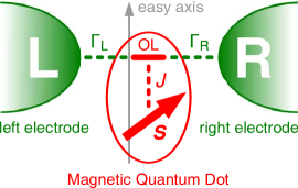
Figure 1: (Color online) Schematic depiction of the system under consideration. It consists of a single orbital level (OL) tunnel-coupled to external leads, with coupling strengths $\Gamma_{L}$ and $\Gamma_{R}$ for the left and right leads, and additionally exchanged-coupled to a spin $S$, with $J$ denoting the strength of exchange interaction.

The magnetic quantum dot is assumed to be tunnel-coupled to two identical electrodes only via the orbital level, see Fig. 1, and electrons in the $q$th electrode [$q=\$(L)eft, (R)ight] are modelled by, $\mathcal{H}_{\textrm{el}}^{q}=\sum_{\sigma}\int_{-W}^{W}\textrm{d}\epsilon\,\epsilon\,a_{q\sigma}^{\dagger}(\epsilon)a_{q\sigma}(\epsilon)$, with $a_{q\sigma}^{\dagger}(\epsilon)$ being the relevant creation operator, and $W$ the band half-width. The electron tunneling processes between the MQD and electrodes are described by

$$\mathcal{H}_{\textrm{tun}}=\sum_{q\sigma}\sqrt{\frac{\Gamma_{q}}{\pi}}\int_{-W}^{W}\textrm{d}\epsilon\,[a_{q\sigma}^{\dagger}(\epsilon)c_{\sigma}+c_{\sigma}^{\dagger}a_{q\sigma}(\epsilon)],$$ (2)

where $\Gamma_{q}$ represents the strength of coupling of the orbital level to the $q$th lead.

Conceptually, the model considered is equivalent to a single-level quantum dot which – if occupied by a single electron – is exchanged coupled to a large-spin magnetic impurity subject to magnetic anisotropy. Kusunose and Miyake (1997) Moreover, to some extent it can be regarded as an alternative to a two-impurity Kondo model where only one impurity couples directly to conduction band, or to a double quantum dot system in a T-shape geometry. Vojta et al. (2002); Cornaglia and Grempel (2005); Chung et al. (2008); Žitko (2010) From this point of view our model will also exhibit a two-stage Kondo effect and a quantum phase transition, as shall be discussed in next section.

Generally, the physics of the Kondo effect is essentially determined by the number of conduction-electron channels to which the system is coupled, as in order to completely screen a spin $S$ one needs $2S$ channels. Nozières and Blandin (1980) In this context, high-spin molecular devices are unique as they commonly operate in the regime where effectively only one channel plays a role. Parks et al. (2010); Florens et al. (2011) More precisely, even if the device is coupled to multiple leads, each of such junction usually supports only a single conduction channel, and additionally the couplings are typically characterized by a strong asymmetry. As a result, the relevant Kondo energy scale is determined by the strongest coupling, since the Kondo temperatures associated with weaker couplings are exponentially small, Haldane (1978) and hence negligible under typical experimental conditions. In the model considered here the situation is even simpler, since the orbital level of magnetic quantum dot couples only to an even linear combination of the electron operators in the left and right leads, with a new coupling strength $\Gamma\equiv\Gamma_{L}+\Gamma_{R}$, while the odd combination is completely decoupled. This basically means that we can limit our discussion to the case of a single conduction-electron channel.

In the following, we will study the linear-response transport properties of magnetic quantum dots on various parameters of the system. The main quantity we are interested in is the temperature-dependent linear conductance $G$, which we calculate from the Landauer-Wingreen-Meir formula, Landauer (1970); Meir and Wingreen (1992)

$$G=\frac{2e^{2}}{h}\sum_{\sigma}\frac{2\Gamma_{L}\Gamma_{R}}{\Gamma_{L}+\Gamma_{R}}\int\!\textrm{d}\omega\left(\!-\frac{\partial f(\omega)}{\partial\omega}\right)\pi A_{\sigma}(\omega),$$ (3)

where $f(\omega)$ denotes the Fermi-Dirac distribution function, while $A_{\sigma}(\omega)$ is the spin-dependent spectral function of the orbital level, and $2\Gamma_{L}\Gamma_{R}/(\Gamma_{L}+\Gamma_{R})=\Gamma/2$ in the present situation. The problem of determining the MQD’s transport features corresponds then essentially to finding the spin-resolved spectral function $A_{\sigma}(\omega)$, which in the present work is obtained by means of the Wilson’s numerical renormalization group (NRG) method. Wilson (1975); Bulla et al. (2008) In particular, we employ the recent idea of a full density matrix, Weichselbaum and von Delft (2007) which allows for reliable calculation of static and dynamic properties of the system at arbitrary temperatures. Legeza et al. (2008) For the present problem, to obtain decent results, the $U_{\textrm{charge}}(1)\times U_{\textrm{spin}}(1)$ symmetry was exploited, the discretization parameter $\Lambda=1.8$ was used and we kept $N_{k}=1200$ states during calculations.

III Results and discussion

In this paper we consider the transport features of a prototypical magnetic quantum dot characterized by the spin $S=2$. The other parameters are typical of molecular systems, see the caption of Fig. 2. In order to discuss the influence of finite temperature on the Kondo effect, we introduce the Kondo temperature $T_{\textrm{K}}$, to which other parameters will be compared whenever it is useful. The Kondo temperature is defined here as the half-width at the half-maximum of the normalized linear conductance $G/G_{T,J,D=0}$ as a function of $T$, where $G_{T,J,D=0}$ is the conductance for $T=D=J=0$, which yields $T_{\textrm{K}}/U\approx 5\cdot 10^{-3}$.

III.1 The case of zero magnetic anisotropy ($D=0$)

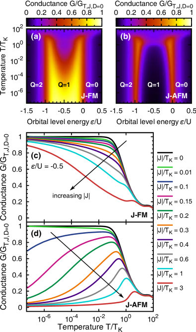
Figure 2: (Color online) The dependence of the linear conductance $G$ on the energy of the orbital level (OL) $\varepsilon$ and the temperature $T$ in the case of (a,c) ferromagnetic (FM) and (b,d) antiferromagnetic (AFM) exchange coupling $J$ for $|J|/T_{\textrm{K}}=3$ and $D=0$. The variable $Q$ represents the average number of electrons that occupy the OL. Here, $G_{T,J,D=0}$ corresponds to the conductance calculated for $T=D=J=0$. Parts (c)-(d) present the relevant cross-sections of the density plots at the electron-hole symmetry point ($\varepsilon=-U/2$) for different values of the $J$-coupling, as indicated. The parameters of the system are as follows: $U=10$ meV, $\Gamma/U=0.1$ and $T_{\textrm{K}}/U\approx 5\cdot 10^{-3}$.

Before the influence of the magnetic anisotropy on the temperature dependence of the Kondo effect is analyzed, it is instructive to consider the situation with vanishing magnetic anisotropy, $D=0$. The corresponding results are shown in Fig. 2, which presents the dependence of the linear conductance on orbital level position and temperature for different exchange couplings $J$. It can be seen that when the orbital level is occupied by even number of electrons, which corresponds to an empty or fully occupied level, the conductance is generally suppressed and determined only by elastic cotunneling processes, see Figs. 2(a,b). On the other hand, for an odd occupation of the orbital level (single spin regime), the Kondo effect should in general develop at low temperatures. Now, however, the exchange interaction with the core spin $S$ comes into play. In principle, two distinctive cases with respect to the $J$-coupling sign can be recognized. For the ferromagnetic exchange coupling, the low temperature behavior of the system is governed by the competition between the coupling $J$ and hybridization with electrodes $\Gamma$. The former interaction tends to stabilize the high-spin state, whereas the later one leads to the screening of the orbital level’s spin. It has been shown for a system including two spin-1/2 impurities, that the Kondo effect dominates even if the exchange coupling is significantly larger than the hybridization. Kusunose and Miyake (1997); Izumida et al. (1998) This can be also seen in Fig. 2(c), where irrespective of the magnitude of $J$, $G$ tends to its maximum value in the zero temperature limit. Nevertheless, the exchange interaction still plays a prominent role, because it is responsible for the reduction of the Kondo temperature, as compared to a simple spin-1/2 magnetic impurity system.

The situation is qualitatively different for antiferromagnetic $J$-coupling. Investigations of high-spin two-impurity (with spins $S_{1}$ and $S_{2}$) Kondo models characterized by the antiferromagnetic inter-impurity exchange interaction and only one impurity ($S_{1}$) directly coupled to a conduction band have revealed a two-stage Kondo effect which is a generic feature for all $S_{2}\geqslant S_{1}$ models. Žitko (2010) In particular, a two-stage Kondo process should take place for the inter-impurity exchange coupling smaller than the energy scale $T_{\textrm{K}}$ associated with the Kondo screening of the directly coupled impurity. For $S_{1}=1/2$, the temperature $T_{\textrm{K}}^{\prime}$ at which $S_{2}$ becomes screened is then exponentially smaller, as the process occurs due to interaction of $S_{1}$ with a Fermi sea arising as a consequence of the first screening stage. Cornaglia and Grempel (2005) The two-stage Kondo effect can be nicely seen in Fig. 2(d), which shows the temperature dependence of linear conductance for different antiferromagnetic exchange coupling. Let us have a closer look at the curve corresponding to $|J|/T_{K}=0.2$. For $T<T_{K}$, the conductance starts increasing due to the Kondo effect associated with the screening of the orbital level spin by conduction electrons. However, at sufficiently low temperatures the energy scale related with the second stage of screening becomes relevant and the conductance becomes suppressed. Moreover, when varying the strength of the exchange interaction at zero temperature, the system undergoes a quantum phase transition. This phase transition is similar to a singlet-triplet transition observed in multilevel quantum dots, Hofstetter and Schoeller (2001); Kogan et al. (2003); Hofstetter and Zarand (2004); Pustilnik and Borda (2006); Roch et al. (2008); Florens et al. (2011) and for finite temperature, magnetic field or anisotropy turns into a crossover.

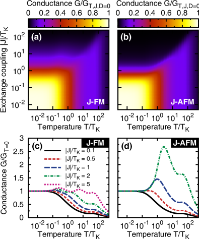
Figure 3: (Color online) The normalized linear conductance $G$ as a function of temperature $T$ and exchange coupling parameter $J$ in the case of (a,c) ferromagnetic (FM) and (b,d) antiferromagnetic (AFM) type of the coupling between magnetic core and orbital level shown in the presence of uniaxial magnetic anisotropy, $D/U=10^{-4}$ ($D/T_{\textrm{K}}=0.2$). Curves in (c)-(d) represent cross-sections of figures (a) and (b), respectively, for indicated values of $|J|$, but now each curve is normalized to the corresponding $G_{T=0}$ instead of $G_{T,J,D=0}$ as in (a)-(b). The other parameters are the same as in Fig. 2 with $\varepsilon=-U/2$.

III.2 The case of finite magnetic anisotropy ($D>0$)

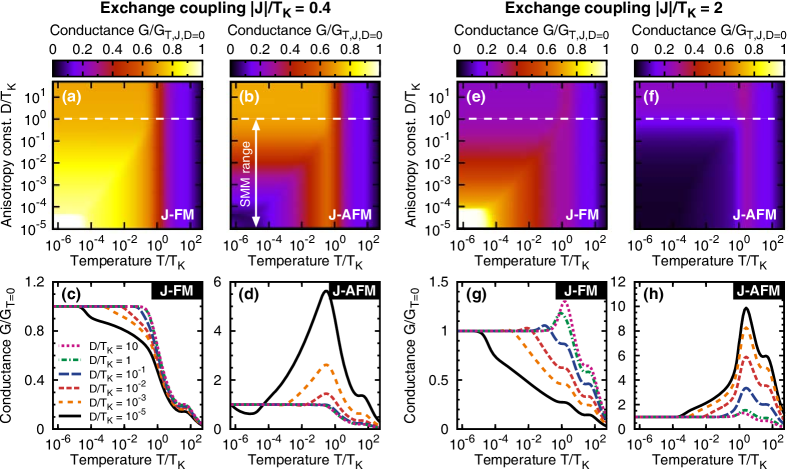
Figure 4: (Color online) The normalized linear conductance $G$ as a function of temperature $T$ and uniaxial magnetic anisotropy $D$ for $|J|/T_{\textrm{K}}=0.4$ in (a)-(d) and $|J|/T_{\textrm{K}}=2$ in (e)-(h). The other parameters are the same as in Fig. 2 with $\varepsilon=-U/2$. Dashed lines in (a)-(b) and (e)-(f) represent maximal value of the uniaxial magnetic anisotropy constant $D$ typical to molecular magnets, for further details see the text.

In the case of finite magnetic anisotropy $D$, the situation becomes more complex since now the degeneracy of spin multiplets is partially lifted. More precisely, in the absence of magnetic anisotropy $D$, the ground state of the MQD is the spin multiplet $S+\frac{1}{2}$ ($S-\frac{1}{2}$) for ferromagnetic (antiferromagnetic) exchange interaction $J$. In the case of finite magnetic anisotropy ($D>0$), the ground state becomes two-fold degenerate and consists of the lowest-weight and highest-weight components of the above multiplets, respectively. Misiorny et al. (2011b)

Figure 3 presents the dependence of the system’s linear conductance $G$ on the exchange coupling $J$ and temperature $T$, for the ferromagnetic and antiferromagnetic types of the $J$-coupling. As long as $|J|\ll T_{\textrm{K}}$, the temperature behavior of the conductance does not differ from that for a typical single-level quantum dot, van der Wiel et al. (2000b); Kretinin et al. (2011); Weymann (2011) see the parts (a) and (b) in Fig. 3. The conductance also does not depend on the sign of the parameter $J$, compare the solid lines (for $|J|/T_{K}=0.1$) in Fig. 3(c)-(d). In such a limit, electrons tunneling through the orbital level are hardly affected by the presence of the MQD’s magnetic core. However, as $|J|\gtrsim T_{\textrm{K}}$, the screening of the orbital level’s spin by conduction electrons is suppressed due to the strong exchange interaction of the orbital level’s spin with the magnetic core. One can then observe that while for $T\ll T_{\textrm{K}}$ the conductance $G$ just decreases monotonically with increasing $|J|$, some additional features of $G$ emerge for $T\sim T_{\textrm{K}}$, see Figs. 3(c)-(d). This stems from the fact that for large $|J|$ the influence of the magnetic core on the orbital level cannot be neglected, as the tunneling processes actually take place via the molecular spin states formed due to the $J$-coupling.

Since transport properties of the magnetic quantum dot in the linear response regime depend basically on the system’s ground state, thus for $|J|\gtrsim T_{\textrm{K}}$, it is the sign of the exchange parameter $J$ that determines the system’s spin multiplets that plays the dominant role, i.e. $S+1/2$ for ferromagnetic $J$ and $S-1/2$ for antiferromagnetic $J$. Specifically, at low temperatures the MQD with ferromagnetic $J$ is found to occupy the doublet state $S_{z}=\pm 5/2$ of the spin multiplet $S=5/2$, whereas under the same conditions the system with antiferromagnetic $J$ prefers the state $S_{z}=\pm 3/2$ belonging to the spin multiplet $S=3/2$. Noting this, the characteristic behavior of the linear conductance for temperatures around $T_{\textrm{K}}$ in Fig. 3 can be explained straightforwardly. In general, the conductance displays additional features (peaks) whenever the number of MQD’s states participating in electronic transport changes due to increased temperature. For this reason, as soon as $T\sim D$, the neighboring states of the same spin multiplet become accessible for electron tunneling processes, and when $T$ reaches the value of $|J|$, $T\sim|J|$, also the states of the other spin multiplet enter into consideration. At these temperatures the linear conductance displays additional peaks, see Figs. 3 (c)-(d). Nevertheless, it should be emphasized that energies of the MQD’s states with the orbital level occupied by a single electron generally depend both on $J$ and $D$. Misiorny et al. (2011b)

Additional feature visible in Fig. 3 is an asymmetry between the ferromagnetic and antiferromagnetic coupling $J$. Note, however, that the value of $G_{T=0}$, to which the conductance in Figs. 3 (c)-(d) is normalized, is different in both cases, and the difference is visible only if $|J|\gtrsim T$, otherwise the thermal fluctuations smear the difference between the cases of ferromagnetic and antiferromagnetic exchange coupling, Figs. 3 (a)-(b). This is related to different spin multiplets relevant for spin flip processes that drive the Kondo effect at low temperatures. Misiorny et al. (2011b)

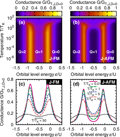
Figure 5: (Color online) The normalized linear conductance $G$ as a function of temperature $T$ and orbital level position $\varepsilon$. Parts (c)-(d) present the relevant cross-sections of the density plots for different temperatures, as indicated. The parameters are the same as in Fig. 2 with $|J|/T_{K}=3$ and $D/T_{K}=0.2$.

Let us now focus on the effects due to the magnetic anisotropy $D$, see Fig. 4. It is worth noting that the anisotropy constant in SMMs can take different values, e.g. in the case of a Fe₄ molecule one finds $D/U\approx 5\cdot 10^{-3}$. This is actually one of the highest values of $D$ observed in SMMs. On the other hand, in magnetic adatoms, such as e.g. Fe, Hirjibehedin et al. (2007) this constant can be as large as $D/U\sim 0.1$. Therefore, we study the effects resulting from magnetic anisotropy and finite temperature for a broad range of anisotropy constant. Figure 4 shows the linear conductance vs. temperature and anisotropy constant for both positive and negative exchange coupling $J$. It can be seen that significant differences between the case of the ferromagnetic and antiferromagnetic $J$-coupling occur for $D\ll|J|$. When the anisotropy is weak, the behavior of linear conductance is the same as discussed previously in the case of $D=0$, i.e. at low temperatures the system is in the underscreened Kondo regime for ferromagnetic $J$-coupling, while for the antiferromagnetic $J$-coupling one observes a two-stage Kondo effect. When the anisotropy increases, see e.g. the case of $D=T_{K}$, both the underscreened and two-stage Kondo effects become generally suppressed. Moreover, the temperature dependence of the normalized linear conductance displays a qualitatively different behavior for the ferromagnetic and antiferromagnetic type of the $J$-coupling. While in the case of ferromagnetic $J$ the increase of $T$ generates a drop of the conductance, see Figs. 4(a,c), the opposite trend appears for antiferromagnetic $J$, see Figs. 4(b,d). This is mainly related with the fact that for a given value of $|J|$, the zero-temperature conductance is much smaller for the antiferromagnetic case than for the ferromagnetic one. Interestingly enough, in both situations one can notice a peak at $T\sim|J|$. For this temperature, the molecular states of another multiplet corresponding to the singly occupied orbital level become available for transport. Because of it, the overall rate of spin-flip processes is increased due to thermal fluctuations and an additional resonance in the conductance appears. Finally, when $D\gtrsim|J|$, the differences between $J<0$ and $J>0$ actually disappear, see the dotted curves for $D/T_{K}=10$ in Figs. 4(c)-(d), which are almost identical. Note that the influence of magnetic anisotropy of the core spin on the transport properties of the system is only present for considerable exchange couplings $|J|\gtrsim T_{K}$.

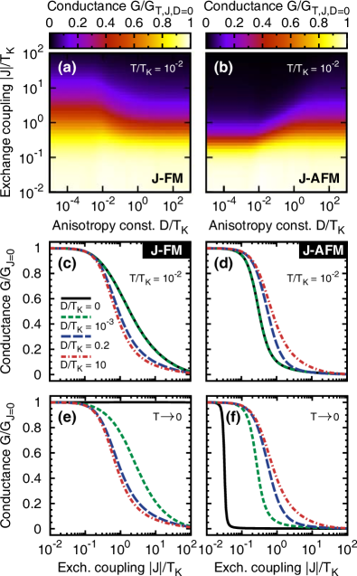
Figure 6: (Color online) Dependence of the normalized linear conductance $G$ on the magnetic anisotropy $D$ and the exchange coupling $J$ of (a) the ferromagnetic (FM) and (b) antiferromagnetic (AFM) type for $T/T_{\textrm{K}}=0.01$. Parts (c) and (d) show the dependence of $G$ on (c) ferromagnetic and (d) antiferromagnetic exchange coupling $J$ for $T/T_{K}=10^{-2}$ and for a few anisotropy constants $D$, as indicated. Parts (e) and (f) show the same calculated for $T\to 0$. The other parameters are the same as in Fig. 2 with $\varepsilon=-U/2$.

It is also interesting to analyze the temperature dependence of the linear conductance in the presence of magnetic anisotropy and for varying position of the orbital level $\varepsilon$, as shown in Fig. 5. The orbital level position can be experimentally tuned by a gate voltage. By changing $\varepsilon$, the orbital level becomes consecutively occupied with electrons, see Fig. 5 where $Q$ denotes the average number of electrons. At low temperatures, $T\ll\Gamma$, transport for even occupations is mediated by cotunneling processes and conductance is low. For the odd occupation ($Q=1$) and $T<T_{K}$, the Kondo effect should generally develop. It is however suppressed due to finite exchange coupling and magnetic anisotropy. It is very instructive to compare Figs. 5(a)-(b) with Figs. 2(a)-(b), where actually the same dependence is plotted for finite anisotropy (Fig. 5) and for $D=0$ (Fig. 2). It can be seen that the main difference occurs in the case of ferromagnetic exchange coupling, when finite anisotropy leads to the suppression of the Kondo effect and conductance is much lower than in the case of $D=0$. In addition, when $T\sim|J|$, a resonance due to thermally-activated spin-flip processes through other spin multiplets occurs. This effect is more visible in the case of antiferromagnetic $J$. On the other hand, once $T>|J|$, the conductance starts decreasing and the difference between the cases of positive and negative $J$ is diminished.

Finally, we study the normalized linear conductance as a function of the anisotropy constant $D$ and exchange coupling $J$ for a constant temperature, $T/T_{K}=10^{-2}$, see Figs. 6(a)-(b). One can see that the effect of exchange interaction becomes visible when $|J|\gtrsim T_{K}$. If this is the case, then the transport properties also depend on the anisotropy constant $D$. For a fixed value of $|J|$, with $|J|\gtrsim T_{K}$, the conductance becomes suppressed by increasing the anisotropy constant in the case of ferromagnetic exchange interaction, while for antiferromagnetic $J$, the behavior is just opposite – there is an increase of $G$. This tendency is also nicely seen in the cross-sections shown in Figs. 6(c)-(d) for a few anisotropy constants $D$. Generally, the conductance drops with increasing $J$ irrespective of the type of exchange interaction. This is, however, because the curves present $G$ vs. $J$ at finite $T/T_{K}=10^{-2}$. In the case of antiferromagnetic exchange coupling there is a quantum phase transition as $J$ is varied. This can be seen in Fig. 6(f), which was calculated for temperature $T\to 0$. This transition turns into a cross-over in the case of finite $T$ and $D$, see Figs. 6(d) and (f). In the case of ferromagnetic exchange interaction in the absence of magnetic anisotropy and for $T\to 0$, the conductance does not depend on $J$ and equals $2e^{2}/h$, see Fig. 6(e). For finite anisotropy $D$, the degeneracy of the ground state multiplet $S+\frac{1}{2}$ is lifted and the Kondo effect is suppressed once $|J|\gtrsim T_{K}$. On the other hand, if the temperature is finite, then at certain value of ferromagnetic exchange interaction the conductance drops since the screening temperature depends on $J$ and the condition $T<T_{K}$ is not met any more.

IV Summary

We have studied transport properties of magnetic quantum dots coupled to external leads in the Kondo regime. The analyzed system consisted of a spin $S=2$ exchange coupled to a single orbital level that was directly tunnel-coupled to electrodes. In particular, we have focused on the dependence of the linear-response conductance of the system on temperature, orbital level position, magnetic anisotropy and exchange coupling. The calculations were performed with the aid of full density-matrix numerical renormalization group method. In the absence of magnetic anisotropy, the model studied generally exhibits a two-stage Kondo effect and an underscreened Kondo phenomenon, depending on the sign of the exchange coupling. We have shown that these two effects become generally suppressed in the presence of magnetic anisotropy, if the exchange coupling is sufficiently strong, $|J|\gtrsim T_{K}$. We have also shown that the temperature dependence of the conductance depends on the type of exchange coupling $J$. For ferromagnetic coupling, the linear conductance was found to generally decrease with $T$, while for antiferromagnetic coupling, the conductance displayed a maximum for $T\sim|J|$. In addition, the conductance variation with the exchange coupling reveals a quantum phase transition for antiferromagnetic $J$-coupling, which turns into a crossover in the case of finite temperature and magnetic anisotropy.

The model studied in the present paper can be used to describe transport through single-molecule magnets, adatoms or quantum dots exchange-coupled to a large spin $S$. Our results and predictions may be thus relevant for a wide class of molecular devices. Finally, we note that molecular devices are more suitable for observing Kondo-related effects, since they provide larger energy scales, which translates into higher Kondo temperatures, more easily achievable in experiments. Florens et al. (2011)