Chandra X-ray observations of Abell 1835 to the virial radius

Abstract

We report the first Chandra detection of emission out to the virial radius in the cluster Abell 1835 at $z=0.253$. Our analysis of the soft X-ray surface brightness shows that emission is present out to a radial distance of 10 arcmin or 2.4 Mpc, and the temperature profile has a factor of ten drop from the peak temperature of 10 keV to the value at the virial radius. We model the Chandra data from the core to the virial radius and show that the steep temperature profile is not compatible with hydrostatic equilibrium of the hot gas, and that the gas is convectively unstable at the outskirts. A possible interpretation of the Chandra data is the presence of a second phase of warm-hot gas near the cluster’s virial radius that is not in hydrostatic equilibrium with the cluster’s potential. The observations are also consistent with an alternative scenario in which the gas is significantly clumped at large radii.

1 Introduction

The large-scale halo of hot gas provides a unique way to measure the baryonic and gravitational mass of galaxy clusters. The baryonic mass can be measured directly from the observation of the hot X-ray emitting intra-cluster medium (ICM), and of the associated stellar component (e.g. Giodini et al., 2009; Gonzalez et al., 2007), while measurements of the gravitational mass require the assumption of hydrostatic equilibrium between the gas and dark matter. Cluster cores are subject to a variety of non-gravitational heating and cooling processes that may result in deviations from hydrostatic equilibrium, and in inner regions beyond the core the ICM is expected to be in hydrostatic equilibrium with the dark matter potential. At the outskirts, the low-density ICM and the proximity to the sources of accretion results in the onset of new physical processes such as departure from hydrostatic equilibrium (e.g., Lau et al., 2009), clumping of the gas (Simionescu et al., 2011), different temperature between electrons and ions (e.g., Akamatsu et al., 2011), and flattening of the entropy profile (Sato et al., 2012), leading to possible sources of systematic uncertainties in the measurement of masses.

The detection of hot gas at large radii is limited primarily by its intrinsic low surface brightness, uncertainties associated with the subtraction of background (and foreground) emission, and the ability to remove contamination from compact sources unrelated to the cluster. Thanks to its low detector background, Suzaku reported the measurement of ICM temperatures to $r_{200}$ and beyond for a few nearby clusters (e.g. Akamatsu et al., 2011; Walker et al., 2012b, a; Simionescu et al., 2011; Burns et al., 2010; Kawaharada et al., 2010; Bautz et al., 2009; George et al., 2009); to date Abell 1835 has not been the target of a Suzaku observation.

In this paper we report the Chandra detection of X-ray emission in Abell 1835 beyond $r_{200}$, using three observations for a total of 193 ksec exposure time, extending the analysis of these Chandra data performed by Sanders et al. (2010). The radius $r_{\Delta}$ is defined as the radius within which the average mass density is $\Delta$ times the critical density of the universe at the cluster’s redshift for our choice of cosmological parameters. The virial radius of a cluster is defined as the equilibrium radius of the collapsed halo, approximately equivalent to one half of its turnaround radius (e.g. Lacey & Cole, 1993; Eke et al., 1998). For an $\Omega_{\Lambda}$-dominated universe, the virial radius is approximately $r_{100}$ (e.g. Eke et al., 1998). Abell 1835 is the most luminous cluster in the Dahle (2006) sample of clusters at $z=0.15-0.3$ selected from the Bright Cluster Survey. The combination of high luminosity and availability of deep Chandra observations with local background make Abell 1835 and ideal candidate to study its emission to the virial radius. Abell 1835 has a redshift of $z=0.253$, which for $H_{0}=70.2$ km s^-1 Mpc^-1, $\Omega_{\Lambda}=0.73$, $\Omega_{M}=0.27$ cosmology (Komatsu et al., 2011) corresponds to an angular-size distance of $D_{A}=816.3$ Mpc, and a scale of 237.48 kpc per arcmin.

2 Chandra and ROSAT observations of Abell 1835 and the detection of cluster emission beyond $r_{200}$

2.1 Chandra observations

Chandra observed Abell 1835 three times between December 2005 and August 2006 (observations ID 6880, 6881 and 7370), with a combined clean exposure time of 193 ks. The three observations had similar aimpoint towards the center of the cluster (R.A. 14h01m02s, Dec. +02d51.5m J2000) and different roll angles. All observations were taken with the ACIS-I detector configuration, which consists of four ACIS front-illuminated chips in a two-by-two square, plus a fifth identical chip that may be used to measure the in situ soft X-ray background. Figure 1 is an image from the longest observation (ID 6880, 118ks) in the soft X-ray band (0.7-2 keV). In addition to a large number of compact X-ray sources that were excluded from further analysis, the data show a clear detection of diffuse X-ray emission associated with two additional low-mass clusters identified from the Sloan Digital Sky Survey, MAXBCG J210.31728+02.75364 and WHL J140031.8+025443. The cluster MAXBCG J210.31728+02.75364 is the only cluster in the vicinity of Abell 1835 reported in the MAXBCG catalog of Koester et al. (2007), and it has a measured photo-$z$ of 0.238, while the catalog of Wen et al. (2009) reports a photo-$z$ of 0.269 for the same source; given the uncertainties associated with photometric redshifts, it is likely that the cluster is in physical association with Abell 1835 ($z=0.253$). The Wen et al. (2009) catalog also reports another optically-identified cluster in the area, WHL J140031.8+025443, with a spectroscopic redshift of $z=0.2505$. The association of these two groups with Abell 1835 is confirmed by redshift data provided by C. Haines (personal communication), who measures a redshift of $z=0.250$ for WHL J140031.8+025443, and $z=0.245$ for MAXBCG J210.31728+02.75364.

Since the goal of this paper is to study the diffuse emission associated with Abell 1835, we excise a region of radius 90 arcsec around the position of the two clusters (black circles in Figure 1), and study their emission separately from that of Abell 1835 (see Section 3.2).

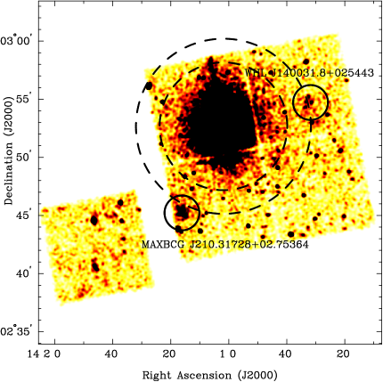
Figure 1: Image of Abell 1835 from observation 6880, in the 0.7-2 keV band. The data were smoothed with a Gaussian kernel of $\sim$6 arcsec standard error. The dashed circles correspond to radial distances of approximately $r_{500}$ and $r_{200}$, and the full black circles mark the position of the two low-mass clusters associated with Abell 1835.

2.2 Chandra data analysis

The reduction of the Chandra observations follow the procedure described in Bonamente et al. (2006) and Bonamente & Nevalainen (2011), which consists of filtering the observations for possible periods of flaring background, and applying the latest calibration; no significant flares were present in these observations. The reduction was performed in CIAO 4.2, using CALDB 4.3; in Sec. 3.3 we discuss the impact of calibration changes on our results. One of the calibration issues that can affect the measurement of cluster emission is the uncertainty in the contamination of the optical blocking filter, which causes a reduction in the low energy quantum efficiency of the Chandra detectors. The spatial and time dependence of this contaminant affects primarily the effective area at $\leq$0.7 keV , with an estimated residual error of $\leq$ 3% at higher energy. We therefore limit our spatial and spectral analysis to the $\geq$0.7 keV band. The superior angular resolution of the Chandra mirrors (Weisskopf et al., 2000) results in a point-spread function with a 0.5 arcsec FWHM, and therefore there is negligible contribution from the bright cluster core to the emission in the outer annuli, and from secondary scatter (stray light) by sources outside the field of view.

The subtraction of particle and sky background is one of the most crucial aspects of the analysis of low surface brightness cluster regions. We use Chandra blank-sky background observations, rescaled according to the high- energy flux of the cluster, to ensure a correct subtraction of the particle background that is dominant at $E\geq 9.5$ keV, where the Chandra detectors have no effective area. The temporal and spatial variability of the soft X-ray background at $E<2$ keV also requires that a peripheral region free of cluster emission is used to measure any local enhancement (or deficit) of soft X-ray emission relative to that of the blank-sky fields, and account for this difference in the analysis. This method is accurate for the determination of the temperature profile, but may result in small errors in the measurement of the surface brightness profile. In fact, the blank-sky background is a combination of a particle component that is not vignetted, and a sky component that is vignetted. To determine the surface brightness of the cluster and of the local soft X-ray background, a more accurate procedure consists of subtracting the non-vignetted particle component as measured from Chandra observations in which the ACIS detector was stowed (e.g., Hickox & Markevitch, 2007), after rescaling the stowed background to match the $E\geq 9.5$ keV cluster count rate, as in the case of the blank-sky background.

Point sources are identified and removed using a wavelet detection method that correlates the cluster observation with wavelet functions of different scale sizes (wavdetect in CIAO). Subtraction of point soures from the blank-sky observations were performed by eye, with results that closely match those of the wavelet method.

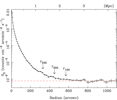
Figure 2: Exposure corrected surface brightness profile of Abell 1835 in the soft X-ray band (0.7-2 keV), obtained by subtraction of the particle background from the ACIS stowed observations. The radii $r_{500}$, $r_{200}$ and the virial radius ($\sim r_{100}$) are estimated from the data in Section 4.2 (see Table 4). The dashed red line is the average background level in the region $\geq$ 700 arcsec.

2.3 Measurement of the surface brightness profile with Chandra

The surface brightness profile obtained using this background subtraction is shown in Figure 2, in which the red line represents the average value of the background at radii $\geq$ 700 arcsec, where the surface brightness profile is consistent with a constant level. To determine the outer radius at which Chandra has a significant detection of the cluster, we also include sources of systematic errors in our analysis. One source of uncertainty is the error in the measurement of the background level, shown in Figure 3 as the solid red lines. The error is given by the standard deviation of the weighted mean of the datapoints at radii greater than 700 arcsec, to illustrate that each bin in the surface brightness profile beyond this radius is consistent with a constant level of the background.

Another source of uncertainty is the amount by which the stowed background is to be rescaled to match the cluster count rate at high energy. The stowed background dataset applicable to the dates of observation of Abell 1835 has an exposure time of 367 ksec, and the relative error in the rescaling of the background to match the cluster count rate at high energy is 0.7%, as determined by the Poisson error in the photon counts at high energy. Moreover, Hickox & Markevitch (2006) has shown that the spectral distribution of the particle background is remarkably stable, even in the presence of changes in the overall flux, and that the ratio of soft-to-hard (2-7 keV to 9.5-12 keV) count rates remains constant to within $\leq$2 %. We therefore apply a systematic error of 2 % in the stowed background flux, to account for this possible source of uncertainty, in addition to the 0.7% error due to the uncertainty in the rescaling of the background.

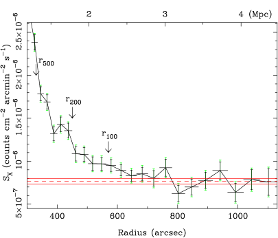
Figure 3: Close-up view of Figure 2, in which the red lines represent the 1-$\sigma$ confidence in the background level as determined from the $\geq$700 arcsec region, and the green error bars combine the statistical and systematic errors in the determination of the surface brightness.

In Figure 3 the green error bars represent the cumulative effect of the statistical error due to the counting statistic, and the sources of errors associated with the use of the stowed background; the systematic errors were added linearly to the statistical error as a conservative measure. This error analysis shows that the emission from Abell 1835 remains significantly above the background beyond $r_{200}$ and until approximately a radius of 600 arcsec, or approximately 2.4 Mpc. The significance of the detection in the region 450-600” (the five datapoints in Figure 3 after the $r_{200}$ marker) is calculated as 5.5$\sigma$, and is obtained by using the larger systematic error bars for the surface brightness profile (in green in Figure 3), added in quadrature to the error in the determination of the background level from the $\geq 700$” region (red lines in Figure 3).

To further test the effect of the background subtraction, we repeat our backround subtraction process using the $\geq 600$” region (instead of the $\geq 700$” region) . The background level increases by less than 1$\sigma$ of the value previously determined (e.g., the two levels are statistically indistinguishable), and the significance of detection in the region 450-600” is 4.7$\sigma$. Therefore we conclude that it is unlikely that the excess of emission beyond $r_{200}$ and out to the virial radius is due to errors in the background subtraction process. A similar result can be obtained including the 2-7 keV band, but the signal-to-noise is reduced because at large radii this band is dominated by the background due to the softening of the cluster emission. We estimate $r_{200}$ and the virial radius ($\sim r_{100}$) from the Chandra data in Section 4.2.

2.4 Measurement of the surface brightness profile with the ROSAT Position Sensitive Proportional Counter

ROSAT observed Abell 1835 on July 3–4 2003 for 6 ks with the Position Sensitive Proportional Counter (PSPC), observation ID was 800569. The PSPC has a 99.9% rejection of particle background in the 0.2-2 keV band (Plucinsky et al., 1993) and an average angular resolution of $\sim$30 arcsec that makes it very suitable for observations of low surface brightness objects such as the outskirts of galaxy clusters (e.g. Bonamente et al., 2001, 2002, 2003). We reduce the event file following the procedure described in Snowden et al. (1994) and Bonamente et al. (2002), which consists of corrections for detector gain fluctuations, and removal of periods with a master veto rate of $\leq$170 counts s^-1 in order to discard periods of high background. These filters result in a clean exposure time of 5.9 ks.

Since the PSPC background is given only by the photon background, we generate an image in the 0.2-2 keV band and use the exposure map to correct for the position–dependent variations in the detector response and mirror vignetting. We masked out the two low-mass cluster regions as we did for the Chandra data and all visible point sources, and obtained and exposure-corrected surface brightness profile out to a radial distance of $\sim$20 arcmin, which corresponds to the location of the inner support structure of the PSPC detector. The ROSAT surface brightness profile therefore covers the entire azimuthal range. In Figure 4 we show the radial profile of the surface brightness in the 0.2-2 keV band, showing a $\sim$2 $\sigma$ excess of emission in the 400-600” region using the background level calculated from the region $\geq$700”, as done for the Chandra data. The ROSAT data therefore provide additional evidence of emission beyond $r_{500}$ and out to the virial radius, although the short ROSAT exposure does not have sufficient number of counts to provide a detection with the same significance as in the Chandra data.

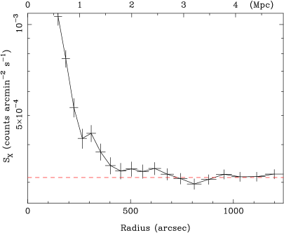
Figure 4: Surface brightness profile in 0.2-2 keV band from a 6 ks observation with ROSAT PSPC. The background level is determined from the data at radii $\geq$ 700”, as in the Chandra data.

3 Analysis of the Chandra spectra

3.1 Measurement of the temperature profile of Abell 1835

We measure the temperature profile of Abell 1835 following the background subtraction method described in Sec. 2, which makes use of the blank-sky background dataset and a measurement of the local enhancement of the soft X-ray background, as is commonly done for Chandra data (e.g. Vikhlinin et al., 2006; Maughan et al., 2008; Bulbul et al., 2010). In Figure 5 we show the spectral distribution of the local soft X-ray background enhancement, as determined from a region beyond the virial radius ($\geq$700 arcsec); this emission was modelled with an APEC emission model of $kT\sim 0.25$ KeV and of Solar abundance, consistent with Galactic emission, and then subtracted from all spectra. The spectra were fit in the 0.7-7 keV band using the minimum $\chi^{2}$ statistic, after binning to ensure that there are at least 25 counts per bin. We use XSPEC version 12.6.0s for the spectral analysys.

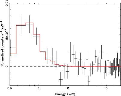
Figure 5: Spectrum of the local enhancement of the soft X-ray background from observation 6880. The other two exposures have similar levels of soft X-ray fluxes above the blank-sky emission, which is modeled as an unabsorbed $\sim 0.25$ keV thermal plasma at $z=0$. The best-fit model has a $\chi^{2}_{min}=73.9$ for 78 degrees of freedom, for a null hypothesis probability of 61%.

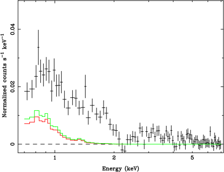
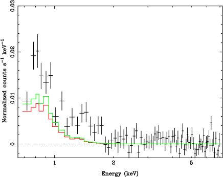
Figure 6: Blank-sky background subtracted spectra of regions 330-450” and 450-600” from observation 6880. The solid lines are the best-fit model of the local soft X-ray enhancement of Figure 5 (red), and its 90% upper limit (green).

In Figure 6 we show the spectra of the outermost two regions, to show the impact of the soft X-ray residuals in the background subtraction. The importance of background systematics in the detection of emission and measurement of cluster temperatures for regions of low surface brightness was recently addressed by Leccardi & Molendi (2008) using XMM-Newton data. For our Chandra observations, the two main sources of uncertainty when determining the temperature of the outer regions are the subtraction of the blank-sky background, and the subtraction of the locally-determined soft X-ray background. Table 1 reports the statistics of the background relevant to the outer regions of the cluster, with both regions $\sim$ 10-20% above the blank-sky background, determined with a precision of 1-2%. The additional soft X-ray background accounts for a significant portion of the remaining signal, as shown in Figure 6; the 90% upper limit to the measurement of this background is shown as the green lines, and emission from the cluster is still detected with high statistical significance. Both sources of error are included in the temperature measurements at large radii.

Table 1: Background levels in outer regions

	Observation ID
	6880	6881	7370
Exposure time (ks)	114.1	36.0	39.5
Correction to Blank-sky Subtractiona	-0.04$\pm$0.01	-0.125$\pm$0.015	-0.04$\pm$0.015
Region 330-450”
Total Counts	18,124	4,938	5,686
Count rate (c s-1)	0.158$\pm$0.001	0.137$\pm$0.002	0.144$\pm$0.002
Net count rateb ($10^{-2}$ c s-1)	$2.75\pm 0.10$	$2.54\pm 0.20$	$2.36\pm 0.20$
Percent above back.	17.4$\pm$0.6	18.2$\pm$1.4	16.4$\pm$1.4
SXB count rate ($10^{-3}$ c s-1)	3.34$\pm$0.77	7.20$\pm$0.94	7.10$\pm$0.71
Region 450-600”
Total Counts	15,811	4,901	5,483
Count rate (c s-1)	0.139$\pm$0.001	0.136$\pm$0.002	0.139$\pm$0.002
Net count rateb ($10^{-2}$ c s-1)	1.02$\pm$0.10	1.58$\pm$0.20	1.23$\pm$0.20
Percent above back.	7.3$\pm$0.7	11.6$\pm$1.5	8.8$\pm$1.4
SXB count rate ($10^{-3}$ c s-1)	3.06$\pm$0.70	7.50$\pm$0.98	7.32$\pm$0.73

We use the APEC code (Smith et al., 2001, code version 1.3.1) to model the Chandra spectra, with a fixed Galactic HI column density of $N_{H}=2.04\times 10^{20}$ cm^-2 (Kalberla et al., 2005). The region at radii $\leq 330$” have a variable metal abundance, while the outer region have a fixed abundance of $A=0.3$. In addition to the statistical errors obtained from the XSPEC fits, we add a systematic error of 10% in the temperature measured in the core and a 5% error to the other region, to account for possible systematic uncertainties due to the Chandra calibration (see, e.g., Bulbul et al., 2010). One possible source of systematic uncertainty in our results is indicated by the systematic difference between the Chandra/ACIS andXMM-Newton/EPIC temperature measurements of galaxy clusters (Nevalainen et al., 2010) This amounts to a $\pm$10% bias in the calibration of the effective area at 0.5 keV, which decreases roughly linearly towards 0% bias at 2 keV. Assuming that XMM-Newton/pn has a more accurately calibrated effective area, we reduced the Chandra effective area by multiplying it with a linear function as indicated by the Chandra/XMM-Newton comparison. As a result, the temperature at the outermost radial bin decreases by $\sim$ 5%. Thus, the cross-calibration uncertainties between Chandra and XMM-Newton do not explain the low temperature we measure in the outermost radial bin. Uncertainties in the Galactic column density of HI do not impact significantly our results. Changing the value of $N_{H}$ by $\pm$10%, consistent with the variations between the Kalberla et al. (2005) and the Dickey & Lockman (1990) measurements, results in a change of best-fit temperature in each bin by less than 2%.

Given the emphasis of this paper on the detection of emission at large radii, we investigate the sources of uncertainty caused by the background subtraction in the outer region at $\geq$330”. We report the results of this error analysis in Table 2, where cornorm refers to the normalization of the blank-sky background, and soft residuals refers to the normalization of the soft X-ray residual model, as reported in Table 1. In the analysis that follows, we add the systematic errors caused by these sources linearly to the statistical error. Our data do not constrain well the metal abundance of the plasma in the outer regions. Using an abundance of $A=0.5$ instead of the nominal $A=0.3$ leads to negligible changes in the best-fit temperature for both of the outer annuli. In the extreme case of an $A=0.0$ metal abundance, both regions have an acceptable fit with the best-fit temperatures change respectively by $+6$% for the 330-450” region ($\Delta\chi^{2}=+1.3$), and by $-22$% for the 450-600” region ($\Delta\chi^{2}=+9.2$, best fit decreases from 1.26 to 0.98 keV). We therefore find that, in the case of exceptionally low metalllicity, the temperature profile we measure from these Chandra data would be even significantly steeper than indicated by the result in Table 2. Given that these data do not provide direct indication that the plasma in the outer regions may have null metal content, we do not fold in this source of systematic error in the analysis that follows.

Table 2: Temperature measurement and error analysis from the Chandra data.

Region	Projected Temperature (keV)
	Measurementa	Calibration errorb
0-10”	4.78$\pm$0.06	$\pm$0.48
10-20”	7.09$\pm$0.14	$\pm$0.71
20-30”	8.72$\pm$0.27	$\pm$0.87
30-60”	9.47$\pm$0.21	$\pm$0.47
60-90”	10.57$\pm$0.33	$\pm$0.53
90-120”	9.97$\pm$0.44	$\pm$0.50
120-180”	9.68$\pm$0.49	$\pm$0.48
180-240”	7.85$\pm$0.65	$\pm$0.39
240-330”	6.02$\pm$0.65	$\pm$0.30
330-450”	3.75$\pm$0.72	$\pm$0.19
450-600”	1.26$\pm$0.16	$\pm$0.06
Measurement of Temperature Using
Background Systematic Errors (keV)
	$+1\sigma$ cornormc	$-1\sigma$ cornorm
330-450”	3.02$\pm$0.54	4.67$\pm$1.00
450-600”	1.09$\pm$0.10	1.31$\pm$0.18
	$+1\sigma$ soft res.d	$-1\sigma$ soft res.
450-600”	4.53$\pm$1.03	3.05$\pm$0.54
450-600”	1.37$\pm$0.25	1.16$\pm$0.12
Summary of Background Systematic Errorse
330-450”	$\pm 0.83\pm 0.74$ keV
450-600”	$\pm 0.11\pm 0.10$ keV

Sanders et al. (2010) measured temperature profiles for Abell 1835 out to approximately $r_{500}$ with Chandra and XMM-Newton. Using the same Chandra observations we analyze in this paper, their temperature profile has a similar drop from the peak value to their outermost annulus ($322\pm 42$”), where they measure a temperature of kT=$4.67\pm^{0.82}_{0.52}$ keV that is consistent with our measurements. Likewise, from the XMM-Newton data their outermost radial bin ($300\pm 10$”) has a temperature of kT=$5.2\pm^{1.2}_{0.7}$ keV, also in agreement with our results. The only measurement of the Abell 1835 temperature to the virial radius available in the literature is that of Snowden et al. (2008), who does report a temperature profile out to a distance of 12 arcmin from a long XMM-Newton observation (and out to 7’ from a shorter observation). In particular, they report a temperature of $kT=3.14\pm 0.93$ for the region 420-540”, which straddles our measurements at 330-450” ($3.75\pm 0.72$ keV) and at 450-600” ($1.26\pm 0.16$, statistical errors only). The same paper also reports a measurement of $kT=3.33\pm 1.75$ keV for the region 540-720”, i.e., beyond our outer annulus. Their temperature is somewhat higher that ours, although the large error bars cannot exclude that the Chandra and XMM-Newton measurements are consistent. Therefore our results confirm and extend the earlier XMM-Newton analysis of Snowden et al. (2008).

3.2 Measurement of the average temperature of MAXBCG J210.31728+02.75364 and WHL J140031.8+025443

We also measure the temperature of the two SDSS clusters detected in our Chandra images, MAXBCG J210.31728+02.75364 and WHL J140031.8+025443. The two clusters are located between a distance of $\sim$380-650” from the cluster center, and therefore we start by extracting a spectrum for this annulus excluding two regions of 1.5’ radius centered at the two clusters. This radius was determined by visual inspection, after smoothing of the Chandra image with a Gaussian kernel of $\sigma=6$ arcsec. For this annulus, we measure a temperature of $kT=1.85\pm 0.36$ keV for a fixed abundance of $A=0.3$ Solar. We then use this spectrum as the local background for the two cluster regions, and measure a temperature $kT=2.73\pm^{0.93}_{0.54}$ keV i for MAXBCG J210.31728+02.75364 (357 source photons, 19% above the average emission of the annulus), and $kT=2.09\pm^{4.6}_{0.55}$ keV for WHL J140031.8+025443 (538 photons, 27% above background). For both clusters, we assumed the same Galactic $HI$ column density as for Abell 1835, and a fixed metal abundance of $A=0.3$ Solar. For both clusters we also extract spectra in regions larger than 1.5’, and determine that no additional source photons are present from these two clusters beyond this radius.

3.3 Tests of robustness of the temperature measurement at large radii

To further test the measurement of temperatures especially at large radii, where the background subtraction is especially important, we also measure the temperature profile using the same stowed background data that was used for the surface brightness measurement of Figures 2 and 3. As in the case of the blank-sky background, we first rescale the stowed data to match the high-energy count rate of the cluster observation, and use a region at large radii ($\geq$ 700 arcsec) to measure the local X-ray background. We model the background using an APEC plus a power-law model, the latter component necessary to model the harder emission due to unresolved AGNs that is typically removed when the blank-sky background is used instead, and apply this model to all cluster regions. We find that the temperature profile is consistent within the 1 $\sigma$ statistical errors of the values provided in Table 2 for each region, and therefore conclude that the temperature drop at large radii, and especially in the outermost region, is not sensitive to the background subtraction method.

The temperature measurement is also dependent on an accurate subtraction of background (and foreground) sources of emission. Point sources in the field of view are detetected using the CIAO tool wavdetect, which correlates the image with wavelets at small angular scales (2 and 4 pixels, one pixel is 1.96”), searches the results for 3-$\sigma$ correlations, and returns a list of elliptical regions to be excluded from the analysis. We study in particular the effect of background sources on the measurement of the temperature in the outermost annulus (450-600”). In this region, wavdetect finds 24 point sources, plus portions of the two low-mass galaxy clusters described in Section 3.2. We extract a spectrum for this region from the longest observation (ID 6880), and now include in the spectrum all point sources excluded in the previous analysis. We find a count rate of $3.20\pm 0.13\times 10^{-2}$ counts s^-1, compared to the point source-subtracted rate of $1.02\pm 0.10\times 10^{-2}$ counts s^-1, corresponding to an increase in background-subtracted flux by a factor of three. We then fit the spectrum with the same APEC model as described in Section 3.1, and find a best-fit temperature of $kT=1.96\pm 0.17$ keV for a best-fit goodness statistic of $\chi^{2}=537$ for 429 degrees of freedom (or $\chi^{2}_{red}$=1.25), compared to the temperature of $1.22\pm 0.19$ keV for a $\chi^{2}=415$ for 389 degrees of freedom (or $\chi^{2}_{red}$=1.08). We therefore conclude that an accurate subtraction of point sources and unrelated sources of diffuse emission is crucial to obtain an accurate measurement of the temperature profile, especially in regions of low-surface brightness such as those near the virial radius.

Changes in the instrument calibration affect the measurement of temperatures. We therefore repeat the same data reduction and spectral analysis using the latest software and calibration database available at time of writing (CIAO 4.4 and CALDB 4.5.1) for the longest observation (ID 6880), and obtain a new temperature profile for the same regions as reported in Table 2. In the outermost two regions, we measure a temperature of 3.04$\pm 0.69$ keV (330-450”) and 1.23$\pm$0.21 keV (450-600”), well within the 1-$\sigma$ confidence intervals of the measurements using the older calibration (3.40$\pm$0.76 and 1.22$\pm$0.19 respectively, also in agreement with the values of Table  2 obtained from the combination of all exposures). The temperature of the inner regions are also always within 1-$\sigma$ of the results obtained with the earlier calibration, and we therefore conclude that changes in the instrument calibration do not affect significantly our results.

4 Measurement of masses and gas mass fraction

We fit the surface brightness and the temperature profiles with the Vikhlinin et al. (2006) model. The electron density is modelled with a double-$\beta$ profile modified by a cuspy core component and an exponential cutoff at large radii, for a total of eleven model parameters; the temperature has both a cool-core component to follow the cooler gas in the core, and a decreasing profile at large radii, for an additional nine parameters. For our analysis, we follow Vikhlinin et al. (2006) and fix the $\gamma$=3.0 parameter, and do not use the cuspy-core component ($\alpha=0$) or the second $\beta$-model component, so that the density is modelled by just one $\beta$-model with an exponential cutoff, for just four free parameters (core radius $r_{c}$, exponent $\beta$, scale radius $r_{s}$ and exponential cutoff exponent $\epsilon$, see Table 3). For the temperature profile, we fix the parameter $a=0$, and the remaining eight parameters are reported in Table 3.

We use a Monte Carlo Markov chain (MCMC) method that we used in previous papers (e.g., Bonamente et al., 2004, 2006). The MCMC analysis consists of a projection of the three-dimensional models and a comparison of the projected surface brightness and temperature profiles, and results in simultaneous estimation of the posterior distributions of all model paramters. Uncertainties in the parameters are obtained from the posterior distributions, with 1-$\sigma$ errors assigned using the 68.3% confidence interval around the median of the distribution.

The gas mass is directly calculated from the electron density model parameters via

$$M_{gas}(r)=m_{p}\mu_{e}\int_{0}^{r}n_{e}(r)4\pi r^{2}dr$$ (1)

and the total gravitational mass via the equation of hydrostatic equilibrium,

$$M(r)=-\frac{kT(r)r}{\mu_{e}m_{p}G}\left(\frac{d\ln n_{e}}{d\ln r}+\frac{d\ln kT}{d\ln r}\right),$$ (2)

where $m_{p}$ is the proton mass, $\mu_{e}\simeq 1.17$ the mean electron molecular weight, and $G$ the gravitational constant. The total density of matter is simply obtained via

$$\rho(r)=\frac{1}{4\pi r^{2}}\frac{dM(r)}{dr}$$

and therefore can be obtained via a derivative of the mass profile. In Equation 2, the term $A=d\ln n_{e}/d\ln r+d\ln kT/d\ln r$ and its first derivative are always negative, as is $dkT(r)/dr$ at large radii. Therefore, the density can be rewritten as

$$\rho(r)=-\frac{1}{4\pi r^{2}\mu_{e}m_{p}G}\left[kT\left(A+r\frac{dA}{dr}\right)+rA\frac{dkT}{dr}\right]$$ (3)

in which the only negative term is the one containing $A\cdot dkT(r)/dr$, while the other two terms remain positive out to large radii.

4.1 Modelling of the Chandra data out to the virial radius

The Vikhlinin et al. (2006) model provides a satisfactory fit out to the outermost radius of 600”; Figure 7 shows the best-fit models to the temperature and surface brightness profiles, best-fit parameters of the model are reported in Table 3. The temperature profile measured by Chandra in Figure 7 is so steep that it causes the total matter density $\rho(r)$ to become negative at approximately 400”, indicating that the temperature profile cannot originate from gas in hydrostatic equilibrium. The situation is illustrated in Figure 8, where the relevant terms of Equation 3 are plotted individually; the density inferred from hydrostatic equilibrium becomes negative where the negative term crosses the positive ones, and the mass profile has a negative slope beyond that point. These fit parameters therefore lead to an unacceptable situation, and responsibility for this inconsistency can be attributed to an overly steep temperature profile, with a drop by a factor of ten between approximately 1.5’ to 10’.

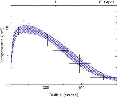
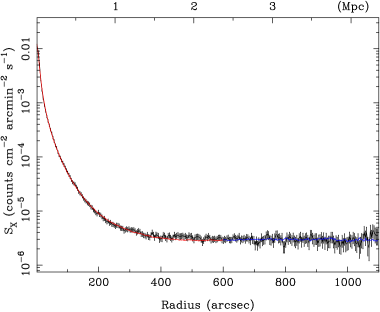
Figure 7: Left: Best-fit Vikhlinin model for the projected temperature profile out to 600”, with 90% confidence intervals. Right: Best-fit Vikhlinin model to the 0.7-2 keV surface brightness (model+background) profile. Emission beyond 600” is statistically consistent with the background, in blue is the extrapolation out to 1100”. Prior removal of the stowed background caused the lower backgroud level in Figure 2.

Table 3: Best-fit parameters for the Vikhlinin model using Chandra data out to 330”

$n_{e0}$	$r_{c}$	$\beta$	$r_{s}$	$\epsilon$	$n_{e02}$	$\gamma$	$\alpha$	$\chi^{2}_{tot}\textrm{(d.o.f.)}$
(10-2cm-3)	(arcsec)		(arcsec)
Using Chandra data out to 330”
$9.602\pm^{0.488}_{0.415}$	$6.743\pm^{0.373}_{0.403}$	$0.498\pm^{0.009}_{0.009}$	$119.8\pm^{13.3}_{13.4}$	$1.226\pm^{0.098}_{0.097}$	0.0	3.0	0.0	$\cdots$
Using Chandra data out to 600”
$9.763\pm^{0.447}_{0.450}$	$6.346\pm^{0.385}_{0.343}$	$0.488\pm^{0.009}_{0.009}$	$96.44\pm^{9.55}_{8.67}$	$1.067\pm^{0.075}_{0.079}$	0.0	3.0	0.0	$\cdots$
$T_{0}$	$T_{min}$	$r_{cool}$	$a_{cool}$	$r_{t}$	$a_{t}$	$b_{t}$	$c_{t}$
(keV)	(keV)	(arcsec)		(arcsec)
Using Chandra data out to 330”
$38.25\pm^{19.63}_{17.23}$	3.0	$92.48\pm^{52.63}_{40.52}$	1.0	$257.5\pm^{143.0}_{66.72}$	0.0	$1.024\pm^{0.426}_{0.283}$	2.0	39.0 (83)
Using Chandra data out to 600”
$10.17\pm^{0.85}_{0.60}$	3.0	$11.82\pm^{3.61}_{2.29}$	$1.924\pm^{0.802}_{0.568}$	600.0	0.0	$2.800\pm^{0.224}_{0.210}$	10.0	106.4 (154)

Table 4: Masses Calculated using Chandra data out to 330”, and Extrapolated out to $r_{100}$

$\Delta$	$r_{\Delta}$	$M_{gas}$	$M_{total}$	$f_{gas}$
	(arcsec)	$\times 10^{13}~{}M_{\odot}$	$\times 10^{14}~{}M_{\odot}$
2500	$164.9\pm^{4.1}_{3.9}$	$4.70\pm^{0.15}_{0.14}$	$5.03\pm^{0.38}_{0.35}$	$0.093\pm^{0.004}_{0.004}$
500	$326.6\pm^{7.1}_{6.9}$	$10.75\pm^{0.23}_{0.23}$	$7.80\pm^{0.52}_{0.49}$	$0.138\pm^{0.006}_{0.006}$
200	$453.3\pm^{15.2}_{15.1}$	$15.36\pm^{0.48}_{0.48}$	$8.35\pm^{0.86}_{0.81}$	$0.184\pm^{0.014}_{0.012}$
100	$570.9\pm^{26.6}_{25.3}$	$19.53\pm^{0.84}_{0.82}$	$8.34\pm^{1.22}_{1.06}$	$0.234\pm^{0.024}_{0.022}$

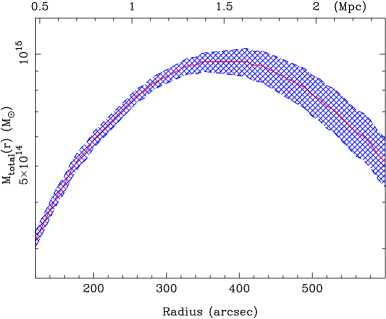
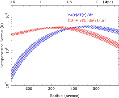
Figure 8: Mass profile using data out to 600” and the temperature fit of Figure 7, and the radial distribution of the positive and negative terms in the density equation (Equation 3).

The results presented in this section provide evidence that the gas detected by Chandra near the virial radius is not in hydrostatic equilibrium, and a number of theoretical studies do in fact suggest that beyond $r_{500}$ the intergalactic plasma is not supported solely by thermal pressure (e.g. Lau et al., 2009). Suzaku has reported the measurement of emission near the virial radius for several clusters, including Abell 1413, Hydra A, Perseus, PKS0745-191, Abell 1795, Abell 1689 and Abell 2029 (Hoshino et al., 2010; Sato et al., 2012; Simionescu et al., 2011; George et al., 2009; Bautz et al., 2009; Kawaharada et al., 2010; Walker et al., 2012b, a). Some of these results do in fact report an apparent decrease in total mass with radius (George et al., 2009; Kawaharada et al., 2010, e.g.) and lack of hydrostatic equilibrium at large radii (e.g. Bautz et al., 2009), similar to the results presented in this paper. Temperature profiles measured by Suzaku typically do not feature as extreme a temperature drop as the one reported in Figure 7, i.e., a factor of nearly 10 from peak to outer radius, although in some cases the drop of temperature from the peak value to that at $r_{200}$ is consistent with the one reported in this paper.

4.2 Modelling of the Chandra data out to $r_{500}$

The steepening of the radial profile beyond 400” is driven by the temperature of the last datapoint beyond $r_{200}$. We also model the surface brightness and temperature profiles of the Chandra data out to only 330”, or approximately $r_{500}$, and find the best-fit Vikhlinin et al. (2006) model for the temperature profile reported in Figure 9 and Table 3. We measure a gas mass fraction of $f_{gas}(r_{500})=0.138\pm 0.006$; if we add the mean stellar fraction as measured by either Giodini et al. (2009) ($f_{\star}=0.019\pm 0.002$) or by Gonzalez et al. (2007) ($f_{\star}\simeq 0.012$) assuming $M(r_{500})=7.1\times 10^{14}$ $M_{\odot}$, we find that Abell 1835 has an average baryon content within $r_{500}$ that is consistent with the cosmic abundance of $\Omega_{b}/\Omega_{M}=0.167\pm 0.007$ (Komatsu et al., 2011) at the 2-$\sigma$ level. As is the case in most clusters, especially relaxed ones, the radial distribution of the gas mass fraction increases with radius (e.g., Vikhlinin et al., 2006).

We use this modelling of the data to measure $r_{500}$, and to provide estimates for $r_{200}$ and the virial radius. The extrapolation of this model to 600” now falls above the measured temperature profile, and the mass profile using hydrostatic equilibrium is monotonic. This best-fit model is marginally compatible with the assumption of hydrostatic equilibrium. In fact, Table 4 shows that the extrapolated mass profile flattens around $r_{200}$, with virtually no additional mass being necessary beyond this radius to sustain the hot gas in hydrostatic equilibrium. Moreover, between $r_{500}$ and $r_{200}$, all of the gravitational mass is accounted by the hot gas mass, i.e., no dark matter is required beyond $r_{500}$. This extrapolation of the $\leq$ $r_{500}$ data to the virial radius therefore leads to a dark matter halo that is much more concentrated than the hot gas.

5 Entropy profile and convective instability at large radii

The Schwarzschild criterion for the onset of convective instability is given by the condition of buoyancy of an infinitesimal blob of gas that is displaced by an amount $dr$, $d\rho_{blob}<d\rho$, where $\rho_{blob}$ is the density of the displaced blob, assumed to attain pressure equilibrium with the surrounding, and $\rho$ is the density of ambient medium. If the blob is displaced adiabatically, using pressure $P$ and entropy $s$ as the independent thermodynamic variables in the derivatives of $\rho_{blob}$ and $\rho$, the buoyancy condition gives

$$\left.\frac{\partial\rho}{\partial s}\right|_{p}ds>0$$ (4)

as condition for convective instability, i.e., a blob that is displaced radially outward will find itself in a medium of higher density and continue to rise to larger radii. Since $({\partial\rho}/{\partial s})_{P}=-\rho^{2}(\partial T/\partial P)_{s}<0$ (material is heated upon adiabatic compression), Equation 4 simply reads that a radially decreasing entropy profile is convective unstable.

An ideal gas has an entropy of

$$S=\nu R\left(\frac{3}{2}\ln T-\ln\rho+C\right)$$ (5)

where $\nu$ is the number of moles, $R$ is the gas constant, and $C$ is a constant. In astrophysical applications, it is customary (e.g. Cavagnolo et al., 2009) to use a definition of entropy that is related to the thermodynamic entropy by an operation of exponential and a constant offset,

$$S=\frac{kT}{n_{e}^{2/3}},$$ (6)

The entropy $S$ defined by Equation 6 has units of keV cm², and it is required to be radially increasing to maintain convective equilibrium. Numerical simulations indicate that entropy outside the core is predicted to increase with radius approximately as $r^{1.1}$ or $r^{1.2}$ (Voit et al., 2005; Tozzi & Norman, 2001). In Figure 10 we show the radial profile of the entropy out to the outer radius of 10 arcmin, with a significant decrease at large radii that indicates an incompatibility of the best-fit model with convective equilibrium. For comparison, we also show the entropy profile measured using the modelling of the data out to only $r_{500}$, as described in Sec. 4.2. This entropy profile uses the shallower temperature profile of Figure 9, and its extrapolation to larger radii remains non-decreasing, i.e., marginally consistent with convective equilibrium.

The Schwarzschild criterion does not apply in the presence of a magnetic field. For typical values of the thermodynamic quantities of the ICM, the electron and ion gyroradii are several orders of magnitude smaller than the mean free path for Coulomb collisions (e.g. Sarazin, 1988), even for a magnetic field of order 1 $\mu G$, and therefore diffusion takes place primarily along field lines (e.g. Chandran & Rasera, 2007). There is strong evidence of magnetic fields in the central regions of clusters (e.g., radio halos, Venturi et al., 2008; Cassano et al., 2006), though it is not clear whether magnetic fields are ubiquitous near the virial radius, as in the case of Abell 3376 (Bagchi et al., 2006). In the presence of magnetic fields, Chandran & Rasera (2007) has shown that the condition for convective instability is simply $dT/dR<0$.

The Chandra data out to the virial radius therefore indicate that the ICM is convectively unstable, regardless of the presence of a magnetic field. In fact, in the absence of magnetic fields near the virial radius, Figure 10 shows that Abell 1835 fails the standard Schwarzschild criterion, i.e., the entropy decreases with radius; in the presence of magnetic fields, the negative gradient in the temperature profile alone is sufficient for the onset of convective instability (e.g., as discussed by Chandran & Rasera, 2007). Convective instabilities would carry hotter gas from the inner regions towards the outer region within a few sound crossing times. As shown by Sarazin (1988), the sound crossing time for a 10 keV gas is $\sim 0.7$ Gyr for a 1 Mpc distance, and an unstable temperature gradient such as that of Figure 7 would be flattened by convection within a few Gyrs. Convection could in principle also result in an additional pressure gradient due to the flow of hot plasma to large radii, which can in turn help support the gas against gravitational forces.

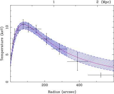
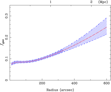
Figure 9: Temperature and gas mass fraction profiles measured from a fit to the Chandra data out to 330”, and extrapolation of the best-fit model out to 600”.

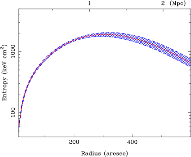
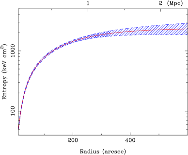
Figure 10: Deprojected entropy profiles using the full Chandra data out to 600” (left, see Section 4.1), and using only data out to $r_{500}$ (right, see Section 4.2).

6 Discussion and interpretation

In this paper we have reported the detection of X-ray emission in Abell 1835 with Chandra that extends out to approximately the cluster’s virial radius. The emission can be explained by the presence of a cooler phase of the plasma that is dominant at large radii, possibly linked to the infall of gas from large-scale filamentary structures. We also investigate the effects of clumping of the gas at large radii, and conclude that in principle a radial gradient in the clumping factor of the hot ICM can explain the apparent flattening of the entropy profile and the turn-over of the mass profile.

6.1 Detection of X-ray emission out to the virial radius

The detection of X-ray emission out to a radial distance of 10 arcmin, or approximately 2.4 Mpc, indicates the presence of diffuse gas out to the cluster’s virial radius. This is the first detection of gas out to the virial radius with Chandra, matching other detections obtained with Suzaku for nearby clusters (e.g. Akamatsu et al., 2011; Walker et al., 2012b, a; Simionescu et al., 2011; Burns et al., 2010; Kawaharada et al., 2010; Bautz et al., 2009; George et al., 2009). Despite its higher background, Chandra provides a superior angular resolution to image and remove emission from unrelated sources. As can be seen from Figure 1, there are approximately 100 point-like sources that were automatically detected and removed, and we were also able to identify two low-mass clusters that are likely associated with Abell 1835. Chandra therefore has the ability to constrain the emission of clusters to the virial radius, especially for higher-redshift cool-core clusters for which the Suzaku point-spread function would cause significant contamination from the central signal to large radii.

It is not easy to interpret the emission at the outskirts as an extension of the hot gas detected at radii $\leq$ $r_{500}$. In fact, as shown in Section 4.1, the steepening of the temperature profile is incompatible with the assumption of hydrostatic equilibrium at large radii. We also showed in Section 5 that the gas has a negative entropy gradient beyond this radius, rendering it convectively unstable. Therefore, if the temperature profile of Figure 7 originates from a single phase of the ICM, convection would transport hotter gas towards the outskirts, flattening the temperature profile within a few Gyrs. Cooling of the gas by thermal radiation cannot be responsible for off-setting the heating by convection, since the cooling time ($t_{cool}\sim kT^{1/2}n_{e}^{-1}$) is longer at the outskirts than in the peak-temperature regions due to the higher density.

6.2 Warm-hot gas towards the cluster outskirts

A possible interpretation for the detection of emission near the virial radius and its steep temperature profile is the presence of a separate phase at the cluster outskirts that is not in hydrostatic equilibrum with the cluster’s potential. In this case, cooler gas may be the result of infall from filamentary structures that feed gas into the cluster, and the temperature of this warm-hot gas may in fact be lower than that shown in Figure 7 (i.e., $kT\sim 1.25$ keV for the region $\geq 450$”) if this gas lies in projection against the tail end of the hotter ICM.

We estimate the mass of this putative warm-hot gas assuming that all of the emission from the outermost region is from a uniform density gas seen in projection. This assumption may result in an overestimate of the emission measure; in fact, the extrapolation of the gas density profile in the hydrostatic or convective scenarios may yield a significant amount of emission in the last radial bin. We were unable to perform a self-consistent modelling of the emission in the full radial range, since the low signal-to-noise ratio does not allow a two-phase modelling in the last radial bin. In this simple uniform density warm-hot gas scenario, the gas is in a filamentary structure of length $L$ and area $A=\pi(R_{out}^{2}-R_{in}^{2})$, where $R_{out}=600$” and $R_{in}=450"$; this is the same model also considered in Bonamente et al. (2005) for the cluster Abell S1101. Since the length $L$ of the filament along the sightline is unknown, we must either assume $L$ or the electron density $n_{e}$, and estimate the mass implied by the detected emission. The emission integral for this region is proportional to

$$K=\frac{10^{-14}}{4\pi D_{A}^{2}(1+z)^{2}}n_{e}^{2}V,$$ (7)

where $K$ is measured in XSPEC from a fit to the spectrum, $D_{A}$ is the angular distance in cm, $z$ is the cluster redshift, and the volume is $V=A\times L$. For this estimate we assume for simplicity that the mean atomic weights of hydrogen and of the electrons are the same, $\mu_{e}=\mu_{H}$. Using the best-fit spectral model with $kT=1.26\pm 0.16$ keV, we measure $K=1.05\pm 0.13\times 10^{-4}$. If we assume a filament of length $L=10$ Mpc, then the average density is $n_{e}=2.4\pm 0.3$ cm^-3, and the filament mass is $4.6\pm 0.6\times 10^{13}$ $M_{\odot}$. Alternatively, a more diffuse filament gas of $n_{e}=10^{-5}$ cm^-3 would require a filament of length $L=58\pm 8$ Mpc, with a mass of $1.1\pm 0.2\times 10^{14}$ $M_{\odot}$, comparable to the entire hot gas mass within $r_{200}$. The fact that a lower density gas yields a higher mass is given by the fact that, for a measured value of $K$ we obtain $n_{e}\propto L^{-1/2}$, and therefore the mass is proportional to $L^{1/2}$. For comparison, the gas mass for this shell inferred from the standard analysis, i.e., assuming that the gas is in the shell itself, is $\sim 3\times 10^{13}$ $M_{\odot}$, as can be also seen from Table 4.

If the gas is cooler, then the mass budget would increase further. In fact, the bulk of the emission from cooler gas falls outside of the Chandra bandpass, and for a fixed number of detected counts the required emission integral increases. We illustrate this situation by fitting the annulus to an emission model with a fixed value of $KT=0.5$ keV, which result in a value of $K=1.88\pm 0.24\times 10^{-4}$ (the fit is significantly poorer, with $\Delta\chi^{2}=+10$ for one fewer degree of freedom). Accordingly, the filament mass estimates would be increased approximately by a factor of two.

A warm-hot phase at $T\leq 10^{7}$ K is expected to be a significant reservoir of baryons in the universe (e.g. Cen & Ostriker, 1999; Davé et al., 2001). Using the ROSAT soft X-ray Position Sensitive Proportional Counter (PSPC) detector – better suited to detect the emission from sub-keV plasma – we have already reported the detection of a large-scale halo of emission around the Coma cluster out to $\sim$ 5 Mpc, well beyond the cluster’s virial radius (Bonamente et al., 2003, 2009). It is possible to speculate that the high mass of Abell 1835, one of the most luminous and massive clusters on the Bright Cluster Survey sample (Ebeling et al., 1998), is responsible for the heating of the infalling gas to temperatures that makes it detectable by Chandra, and that other massive clusters may therefore provide evidence of emission to the virial radius with the Chandra ACIS detectors. The infall scenario is supported by the Herschel observations of Pereira et al. (2010), who measure a galaxy velocity distribution for Abell 1835 that does not appear to decline at large radii as in most of the other clusters in their sample. A possible interpretation for their data is the presence of a surrounding filamentary structure that is infalling into the cluster.

6.3 Effects of gas clumping at large radii

Masses and entropy measured in this paper assume that the gas has a uniform density at each radius. To quantify the effect of departures from uniform density, we define the clumping factor $C$ as the ratio of density averages over a large region,

$$C =\frac{\langle n_{e}^{2}\rangle}{\langle n_{e}\rangle^{2}}$$ (8)

with $C\geqslant 1$. Clumped gas emits more efficiently than gas of uniform density, and the same surface brightness $I$ results in a lower estimate for the gas density and mass,

$$I\propto\int<n_{e}^{2}>dl=\int<n_{e}>^{2}Cdl,$$ (9)

where $l$ is a distance along the sightline. From Figure 10 we see that the entropy drop from approximately 400” to 600” would be offset by a decrease in $n_{e}^{2/3}$ by a factor of 3, or a decrease in $n_{e}$ by a factor of 5. We therefore suggest that a clumping factor of $C\simeq 25$ at 600” would in principle be able to provide a flat entropy profile, and even higher clumping factors would provide an increasing entropy profile in better agreement with theory (e.g. Voit et al., 2005; Tozzi & Norman, 2001). Numerical simulations by Nagai & Lau (2011) suggest values of the clumping factor $C\leq 3$ near $r_{200}$, with significantly higher clumping possible at larger radii. Use of the Nagai & Lau (2011) model in the analysis of a large sample of galaxy clusters by Eckert et al. (2012) results in better agreement of observations with numerical simulations.

Clumping can also affect the measurement of hydrostatic masses. In particular, gas with an increasing radial profile of the clumping factor could result in a steeper gradient of the density profile, when compared with what is measured assuming a uniform density. According to Equation 2, this would result in larger estimates of the hydrostatic mass, in principle able to reduce or entirely offset the apparent decreas of $M(r)$ reported in Figure 8. We therefore conclude that a radial increase in the clumping of the gas can in principle account for the apparent decrease of the mass profile and of the entropy profile reported in this paper (Figures 8 and 10), and therefore it is a viable scenario to interpret our Chandra observations. Clumping of the gas at large radii has also been suggested based on Suzaku observations (e.g., Simionescu et al., 2011).

7 Conclusions

In this paper we have reported the detection of emission from Abell 1835 with Chandra out to the cluster’s virial radius. The cluster’s surface brightness is significantly above the background level out to a radius of approximately 10 arcminutes, which correspond to $\sim$2.4 Mpc at the cluster’s redshift. We have investigated several sources of systematic errors in the background subtraction process, and determined that the significance of the detection in the outer region (450-600”) is $\geq 4.7$ $\sigma$, and the emission cannot be explained by fluctuations in the background. Detection out to the virial radius is also implied by the XMM-Newton temperature profile reported by Snowden et al. (2008).

The Chandra superior angular resolution made it straightforward to identify and subtract sources of X-ray emission that are unrelated to the cluster. In addition to a large number of point sources, we have identified X-ray emission from two low-mass clusters that were selected from the SDSS data, MAXBCG J210.31728+02.75364 (Koester et al., 2007) and WHL J140031.8+025443 (Wen et al., 2009). The two clusters have photometric and spectroscopic redshifts that make them likely associated with Abell 1835. These are the only two SDSS-selected clusters that are in the vicinity of Abell 1835.

The outer regions of the Abell 1835 cluster have a sharp drop in the temperature profile, a factor of about ten from the peak temperature. The sharp drop in temperature implies that the hot gas cannot be in hydrostatic equilibrium, and that the hot gas would be convectively unstable. A possible scenario to explain the observations is the presence of warm-hot gas near the virial radius that is not in hydrostatic equilibrium with the cluster’s potential, and with a mass budget comparable to that of the entire ICM. The data are also consistent with an alternative scenario in which a significant clumping of the gas at large radii is responsible for the apparent negative gradients of the mass and entropy profiles at large radii.

References

- Akamatsu et al. (2011) Akamatsu H., Hoshino A., Ishisaki Y., Ohashi T., Sato K., Takei Y., Ota N., 2011, PASJ, 63, 1019
- Bagchi et al. (2006) Bagchi J., Durret F., Neto G. B. L., Paul S., 2006, Science, 314, 791
- Bautz et al. (2009) Bautz M. W. et al., 2009, PASJ, 61, 1117
- Bonamente et al. (2004) Bonamente M., Joy M. K., Carlstrom J. E., Reese E. D., LaRoque S. J., 2004, Astrophysical Journal, 614, 194
- Bonamente et al. (2006) Bonamente M., Joy M. K., LaRoque S. J., Carlstrom J. E., Reese E. D., Dawson K. S., 2006, Astrophysical Journal, 647, 25
- Bonamente et al. (2003) Bonamente M., Joy M. K., Lieu R., 2003, Astrophysical Journal, 585, 722
- Bonamente et al. (2009) Bonamente M., Lieu R., Bulbul E., 2009, Astrophysical Journal, 696, 1886
- Bonamente et al. (2002) Bonamente M., Lieu R., Joy M. K., Nevalainen J. H., 2002, Astrophysical Journal, 576, 688
- Bonamente et al. (2001) Bonamente M., Lieu R., Mittaz J. P. D., 2001, Astrophysical Journal, Letters, 561, L63
- Bonamente et al. (2005) Bonamente M., Lieu R., Mittaz J. P. D., Kaastra J. S., Nevalainen J., 2005, Astrophysical Journal, 629, 192
- Bonamente & Nevalainen (2011) Bonamente M., Nevalainen J., 2011, Astrophysical Journal, 738, 149
- Bulbul et al. (2010) Bulbul G. E., Hasler N., Bonamente M., Joy M., 2010, Astrophysical Journal, 720, 1038
- Burns et al. (2010) Burns J. O., Skillman S. W., O’Shea B. W., 2010, Astrophysical Journal, 721, 1105
- Cassano et al. (2006) Cassano R., Brunetti G., Setti G., 2006, MNRAS, 369, 1577
- Cavagnolo et al. (2009) Cavagnolo K. W., Donahue M., Voit G. M., Sun M., 2009, Astrophysical Journal, Supplement, 182, 12
- Cen & Ostriker (1999) Cen R., Ostriker J. P., 1999, Astrophysical Journal, 514, 1
- Chandran & Rasera (2007) Chandran B. D. G., Rasera Y., 2007, Astrophysical Journal, 671, 1413
- Dahle (2006) Dahle H., 2006, Astrophysical Journal, 653, 954
- Davé et al. (2001) Davé R. et al., 2001, Astrophysical Journal, 552, 473
- Dickey & Lockman (1990) Dickey J. M., Lockman F. J., 1990, Annual Review of Astronomy and Astrophysics, 28, 215
- Ebeling et al. (1998) Ebeling H., Edge A. C., Bohringer H., Allen S. W., Crawford C. S., Fabian A. C., Voges W., Huchra J. P., 1998, MNRAS, 301, 881
- Eckert et al. (2012) Eckert D. et al., 2012, Astronomy and Astrophysics, 541, A57
- Eke et al. (1998) Eke V. R., Cole S., Frenk C. S., Patrick Henry J., 1998, MNRAS, 298, 1145
- George et al. (2009) George M. R., Fabian A. C., Sanders J. S., Young A. J., Russell H. R., 2009, MNRAS, 395, 657
- Giodini et al. (2009) Giodini S. et al., 2009, Astrophysical Journal, 703, 982
- Gonzalez et al. (2007) Gonzalez A. H., Zaritsky D., Zabludoff A. I., 2007, Astrophysical Journal, 666, 147
- Hickox & Markevitch (2006) Hickox R. C., Markevitch M., 2006, Astrophysical Journal, 645, 95
- Hickox & Markevitch (2007) Hickox R. C., Markevitch M., 2007, Astrophysical Journal, Letters, 661, L117
- Hoshino et al. (2010) Hoshino A. et al., 2010, PASJ, 62, 371
- Kalberla et al. (2005) Kalberla P. M. W., Burton W. B., Hartmann D., Arnal E. M., Bajaja E., Morras R., Pöppel W. G. L., 2005, Astronomy and Astrophysics, 440, 775
- Kawaharada et al. (2010) Kawaharada M. et al., 2010, Astrophysical Journal, 714, 423
- Koester et al. (2007) Koester B. P. et al., 2007, Astrophysical Journal, 660, 239
- Komatsu et al. (2011) Komatsu E. et al., 2011, Astrophysical Journal, Supplement, 192, 18
- Lacey & Cole (1993) Lacey C., Cole S., 1993, MNRAS, 262, 627
- Lau et al. (2009) Lau E. T., Kravtsov A. V., Nagai D., 2009, Astrophysical Journal, 705, 1129
- Leccardi & Molendi (2008) Leccardi A., Molendi S., 2008, Astronomy and Astrophysics, 486, 359
- Marshall et al. (2004) Marshall H. L., Tennant A., Grant C. E., Hitchcock A. P., O’Dell S. L., Plucinsky P. P., 2004, in Society of Photo-Optical Instrumentation Engineers (SPIE) Conference Series, Vol. 5165, Society of Photo-Optical Instrumentation Engineers (SPIE) Conference Series, Flanagan K. A., Siegmund O. H. W., eds., pp. 497–508
- Maughan et al. (2008) Maughan B. J., Jones C., Forman W., Van Speybroeck L., 2008, Astrophysical Journal, Supplement, 174, 117
- Nagai & Lau (2011) Nagai D., Lau E. T., 2011, Astrophysical Journal, Letters, 731, L10
- Nevalainen et al. (2010) Nevalainen J., David L., Guainazzi M., 2010, Astronomy and Astrophysics, 523, A22
- Pereira et al. (2010) Pereira M. J. et al., 2010, Astronomy and Astrophysics, 518, L40
- Plucinsky et al. (1993) Plucinsky P. P., Snowden S. L., Briel U. G., Hasinger G., Pfeffermann E., 1993, Astrophysical Journal, 418, 519
- Sanders et al. (2010) Sanders J. S., Fabian A. C., Smith R. K., Peterson J. R., 2010, MNRAS, 402, L11
- Sarazin (1988) Sarazin C. L., 1988, X-ray emission from clusters of galaxies, Sarazin C. L., ed.
- Sato et al. (2012) Sato T. et al., 2012, ArXiv e-prints
- Simionescu et al. (2011) Simionescu A. et al., 2011, Science, 331, 1576
- Smith et al. (2001) Smith R. K., Brickhouse N. S., Liedahl D. A., Raymond J. C., 2001, Astrophysical Journal, Letters, 556, L91
- Snowden et al. (1994) Snowden S. L., McCammon D., Burrows D. N., Mendenhall J. A., 1994, Astrophysical Journal, 424, 714
- Snowden et al. (2008) Snowden S. L., Mushotzky R. F., Kuntz K. D., Davis D. S., 2008, Astronomy and Astrophysics, 478, 615
- Tozzi & Norman (2001) Tozzi P., Norman C., 2001, Astrophysical Journal, 546, 63
- Venturi et al. (2008) Venturi T., Giacintucci S., Dallacasa D., Cassano R., Brunetti G., Bardelli S., Setti G., 2008, Astronomy and Astrophysics, 484, 327
- Vikhlinin et al. (2006) Vikhlinin A., Kravtsov A., Forman W., Jones C., Markevitch M., Murray S. S., Van Speybroeck L., 2006, Astrophysical Journal, 640, 691
- Voit et al. (2005) Voit G. M., Kay S. T., Bryan G. L., 2005, MNRAS, 364, 909
- Walker et al. (2012a) Walker S. A., Fabian A. C., Sanders J. S., George M. R., 2012a, MNRAS, 424, 1826
- Walker et al. (2012b) Walker S. A., Fabian A. C., Sanders J. S., George M. R., Tawara Y., 2012b, MNRAS, 422, 3503
- Weisskopf et al. (2000) Weisskopf M. C., Tananbaum H. D., Van Speybroeck L. P., O’Dell S. L., 2000, in Society of Photo-Optical Instrumentation Engineers (SPIE) Conference Series, Vol. 4012, Society of Photo-Optical Instrumentation Engineers (SPIE) Conference Series, Truemper J. E., Aschenbach B., eds., pp. 2–16
- Wen et al. (2009) Wen Z. L., Han J. L., Liu F. S., 2009, Astrophysical Journal, Supplement, 183, 197