Numerical simulations of shocks encountering clumpy regions

Abstract

We present numerical simulations of the adiabatic interaction of a shock with a clumpy region containing many individual clouds. Our work incorporates a sub-grid turbulence model which for the first time makes this investigation feasible. We vary the Mach number of the shock, the density contrast of the clouds, and the ratio of total cloud mass to inter-cloud mass within the clumpy region. Cloud material becomes incorporated into the flow. This “mass-loading” reduces the Mach number of the shock, and leads to the formation of a dense shell. In cases in which the mass-loading is sufficient the flow slows enough that the shock degenerates into a wave. The interaction evolves through up to four stages: initially the shock decelerates; then its speed is nearly constant; next the shock accelerates as it leaves the clumpy region; finally it moves at a constant speed close to its initial speed. Turbulence is generated in the post-shock flow as the shock sweeps through the clumpy region. Clouds exposed to turbulence can be destroyed more rapidly than a similar cloud in an “isolated” environment. The lifetime of a downstream cloud decreases with increasing cloud-to-intercloud mass ratio. We briefly discuss the significance of these results for starburst superwinds and galaxy evolution.

1 Introduction

The energy input from high-mass stars in regions of vigorous star formation creates bubbles of hot plasma which may overlap to create superbubbles. Such structures are large enough that they can burst out of their host galaxies, and vent mass and energy into the intergalactic medium. However, the properties of such flows may be dominated by their interaction with components with small volume filling fractions. A complete understanding of the gas dynamics of starburst regions, therefore, requires knowledge of how hot plasma interacts with the cold, dense molecular material present in the interstellar medium and in the superwind.

Material in cold, dense clouds may be incorporated into the hot phase via a variety of processes, including hydrodynamic ablation and thermal or photoionization induced evaporation. This “mass-loading” is a key ingredient in models of galaxy formation and evolution (e.g., Sales et al. 2010), but currently is not calculated self-consistently in these models. The mass-loss rates of clouds are also an important input parameter in models of the ISM (McKee & Ostriker 1977). Alternatively, clouds may be compressed by the high pressure of the hot phase and collapse to form stars.

The response of a cloud to a given set of conditions remains to be fully elucidated. Although a large literature on interactions involving single clouds exists (e.g. Klein et al. 1994; Orlando et al. 2008; Pittard et al. 2009, 2010), there are only a handful of studies on the interaction of a flow overrunning multiple clouds (Jun et al. 1996; Steffen et al. 1997; Poludnenko et al. 2002; Pittard et al. 2005). Thus, there remains a clear need for further studies to examine the collective effects of clouds on a flow, and to determine whether there are differences between the behaviours of upstream and downstream clouds.

This is a first step in a long term study of the global effects of clouds on an overruning flow. To simplify the problem and reduce the number of free parameters we have assumed adiabatic behaviour, with a ratio of specific heats $\gamma=5/3$. It alows us to follow the generic behaviour of a flow interacting with clouds. In future we will perform calculations which include heating and radiative losses. We investigate how cloud destruction affects the density, speed and Mach number of the flow. We also determine whether the position of a cloud within the clumpy region significantly affects its evolution. In Section 2 we describe the numerical code and the initial conditions and a convergence study which informs the subsequent work in this paper. Our results are presented in Section 3, and conclusions and motivation for further work are addressed in Section 5.

2 Method

2.1 Numerical Setup

The computations were performed with the mg hydrodynamic code. This implements adaptive mesh refinement (AMR), a Godunov solver and piecewise linear cell interpolation. The code solves numerically the Euler equations of inviscid flow. These equations are supplemented by a sub-grid turbulent viscosity model, which introduces two additional variables; $k$, the turbulent kinetic energy, and $\epsilon$, its dissipation rate. The fluxes of $k$ and $\epsilon$ across the cell boundaries are also returned by the Riemann solver. The values of $k$ and $\epsilon$ in each cell are updated accordingly, including changes due to source terms. The full set of equations solved can be found in Pittard et al. (2009). The energy source term in eq. 7 of Pittard et al. (2009), $S_{E}$, is $-S_{k}$, defined in eq. 13. $T$ is temperature and $\tau$ is the turbulent stress tensor. More details about the implementation of the $k$-$\epsilon$ model can be found in Falle (1994).

The adopted grids are cartesian, and either 2-D, for clouds that are initially infinite cylinders, or 3-D, for clouds that are initially spheres. We first performed a resolution study for the interaction of a flow with a single cloud. Constant inflow was imposed from the negative $x$-direction together with zero-gradient conditions on the other boundaries. The simulations were terminated before any of the cloud material reached the edges of the grid. In the multi-cloud simulations we imposed periodic boundary conditions in the $y$-direction, with the same inflow and free outflow in the $x$-direction as in the single cloud case.

Two grids ($G^{0}$ and $G^{1}$) cover the entire domain. Finer grids were added where they were needed and removed where they were not, based on the refinement criteria controlled by differences in the solutions on the coarser grids. Each refinement level increased the resolution in all directions by a factor of 2. The time-step on grid $G^{n}$ was $\Delta t_{0}/2n$ where $\Delta t_{0}$ was the time-step on $G^{0}$. The presence of the $k$-$\epsilon$ subgrid model adds a viscous stability condition. The time step is then the smaller of the viscous and hyperbolic time steps. An explicit method is used to advance the solution forwards in time. In single cloud resolution tests, $4$ to $8$ levels of refinement were used with the coarsest $G^{0}$ grid covering the cloud with $0.5-2$ cells per cloud radius, in order to achieve an effective resolution of up to 256 cells per cloud radius. The effective resolution is given by the resolution in the finest grid and is quoted as $R_{cr}$, where cr is the number of cells per cloud radius in the finest grid. For example, $R_{256}$ indicates an effective resolution of $256$ cells per cloud radius. Four levels of refinement were used in the multiple cloud simulations to achieve a resolution of $R_{8}$. All length scales are measured in units of a cloud radius.

The clouds and ambient medium are initially at uniform pressure. Cloud edges have a density profile from Pittard et al. (2009), with $p_{1}=10$. In the single cloud simulations the cloud was centered on the grid origin, and a planar shock front was imposed at $x=-3$. Time zero is defined to be the time when the shock first encounters the cloud. Each simulation is described by the Mach number of the shock, $M$, and the cloud density contrast, $\chi$. The time is measured in units of the cloud crushing timescale, $t_{\rm cc}=\chi^{1/2}r_{\rm cl}/v_{\rm b}$, where $r_{\rm cl}$ is the initial cloud radius and $v_{\rm b}$ is the shock velocity in the ambient medium (Klein et al. 1994). Kelvin-Helmholtz (KH) and Rayleigh-Taylor (RT) instabilities destroy the cloud in $\approx 10\,t_{\rm cc}$ for strong-shock interactions, with weaker shocks taking longer (see Pittard et al. 2010).

In the multiple cloud simulations the clouds are initially randomly distributed within a rectangular region which we refer to as the “clumpy region”. Each cloud has an identical radius and density contrast, and because of the 2D geometry each cloud represents an infinite cylinder. The size of this region is $400\,r_{\rm(cl)}\times 400\,r_{\rm(cl)}$, unless otherwise noted. A key parameter in the multi-cloud simulations is the ratio of total cloud mass to inter-cloud mass in the clumpy region, $MR$. In this work, mass ratios of $MR=0.25-4$ are investigated. Time zero occurs when the shock is just outside the clumpy region, but is often shifted in the subsequent analysis to coincide with the shock entering the region of interest. The clumpy region is divided into 4 equally sized blocks (shown in Fig. 7) with block 1 being furthest upstream and the first to be hit by the shock. Various properties of the total cloud material within a given block and select individual clouds within each block were monitored through the use of advected scalars which “colour” the flow. In pasticular, the velocity and mass of cloud material in individual blocks and clouds are studied. An algorithm which searches for the cells which are furthest downstream and contain a pressure higher than the ambient pressure is used to track the position of the shock as a function of time.

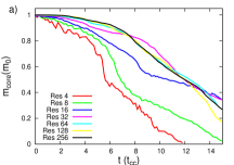
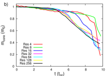
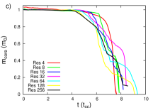
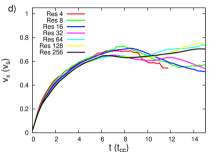
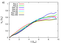
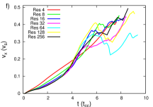
Figure 1: Convergence tests for 2D simulations of a Mach 5 shock hitting a cylindrical cloud with density contrast $\chi=10$ (left column), $\chi=10^{2}$ (center column), and $\chi=10^{3}$ (right column). The time evolution of the core mass (top row) and the mean cloud velocity (bottom row) are shown.

2.2 Convergence Studies

Previous resolution tests of numerical shock-cloud interactions (e.g., Nakamura et al. 2006)) have revealed that adiabatic, hydrodynamic simulations need $\sim 100$ cells per cloud radius ($R_{100}$) for a converged result. Simulations including more complex physics, especially ones with strong cooling, have been found to need higher resolutions (Yirak et al. 2010). In contrast, Pittard et al. (2009) found that adiabatic simulations with a $k$-$\epsilon$ subgrid turbulence model show better convergence, and (most importantly for this work) converge at lower resolutions.

Currently, multiple cloud simulations cannot be performed at a resolution as high as $R_{100}$ and 3D simulations are also much more expensive computationally. The first (and to our knowledge, only) resolution tests of a multiple cloud interaction were performed by Poludnenko et al. (2004), who showed how resolutions of $R_{16}$, $R_{32}$ and $R_{64}$ affect the shock position at a given time. They concluded that the differences between their results were smaller than the sensitivity of their proposed experimental design so no further analysis was done. All the more extensive resolution tests in the current astrophysical literature concern 2D simulations of an individual cloud. We have therefore performed various resolution tests including 2D single cloud simulations with and without a $k$-$\epsilon$ model for different values of $\chi$ and $M$. A 3D single cloud simulation with $M=5$ and $\chi=10^{2}$ was investigated with different resolutions up to $R_{64}$. Multiple (13 and 48) cloud simulations with $M=3$, $\chi=10^{2}$ and $MR=$ 1 and 4 were also performed at resolutions $R_{4}$, $R_{8}$, $R_{16}$ and $R_{32}$.

We focus on two measures which are affected by the mixing of cloud material into the flow. These are the mean cloud velocity ($<v_{x}>$) and the core mass of the cloud ($m_{\rm core}$). The latter is defined as the sum total of cloud mass in grid cells where more than half the cell’s mass is cloud material.

2.2.1 Single cloud resolution tests

Fig. 1 shows the evolution of $m_{\rm core}$ and $<v_{x}>$ for 2D simulations of cylindrical clouds hit by an $M=5$ shock for a range of values of $\chi$.

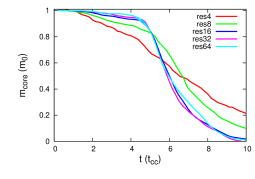
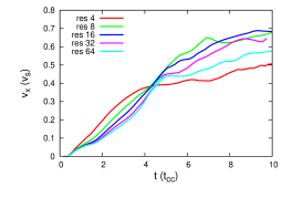
Figure 2: Convergence tests for 3D simulations of a Mach 5 shock hitting a spherical cloud with density contrast $\chi=10^{2}$. The time evolution of the core mass (top) and the mean cloud velocity (bottom) are shown.

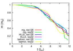
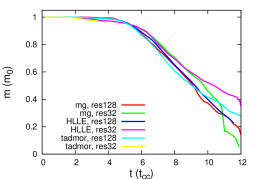
Figure 3: Comparison of the core mass evolution when using the linear/exact Riemann solver in mg and other Riemann solvers. The $k$-$\epsilon$ subgrid model is enabled in the top panel and disabled in the bottom panel. We experienced difficulties with one of the Tadmor calculations which stops at $t=3\,t_{\rm cc}$.

In all cases the interaction leads to most of the core mass being mixed with ambient material by $t\approx 10\,t_{\rm cc}$. The simulations at lower density contrasts are most resolution dependent. When $\chi=10$ the cloud mixes faster at lower resolutions. The opposite is true when $\chi=10^{2}$. For $\chi\mathrel{\hbox to0.0pt{\lower 3.0pt\hbox{$\sim$}\hss}\raise 2.0pt\hbox{$<$}}10^{2}$, simulations with at least 32 cells per cloud radius are much better converged than simulations at lower resolution. For the highest density contrast studied ($\chi=10^{3}$) convergence is obtained at lower resolution.

We now examine the resolution dependence of a spherical cloud in a 3D simulation. Fig. 2 shows the evolution of the core mass and mean cloud velocity as a function of resolution for a cloud with $\chi=10^{2}$ hit by a Mach 5 shock. While the velocity diverges a bit after $5\,t_{\rm cc}$, the core mass evolution at $R_{16}$ exhibits the same features as at $R_{32}$ and $R_{64}$, whereas in 2D a resolution of $R_{32}$ is required for a similar level of convergence. Thus, it appears that the extra degrees of freedom for instabilities in 3D versus 2D has the effect that convergence is achieved at lower resolutions.

The geometry makes a significant difference to the cloud evolution. Panel b of Fig. 1 shows that a cylindrical cloud has lost about half of its core mass by $t\approx 8\,t_{\rm cc}$, whereas Fig. 2 shows that for a spherical cloud this occurs by $t\approx 6\,t_{\rm cc}$.

If the time-averaged pressure returned by the linear solver differs by less than 10% from the pressures in the left and right states, the solution from the linear solver is used. Otherwise an exact solver with the standard Secant method is used. We have compared the effects of different Riemann solvers on single cloud simulations. In particular we have used HLLE (Einfeldt 1988) and Tadmor (Nessyahu & Tadmor 1990) solvers. With a first order (spatial and temporal) update the scheme is very diffusive irrespective of which Riemann solver is used (although the mg solver is least diffusive). Fig. 3 shows results with the standard second order scheme. It reveals that the different solvers produce similar results at high resolutions, while the $k$-$\epsilon$ model reduces the resolution dependance, especially at late times (cf.  Pittard et al. 2009).

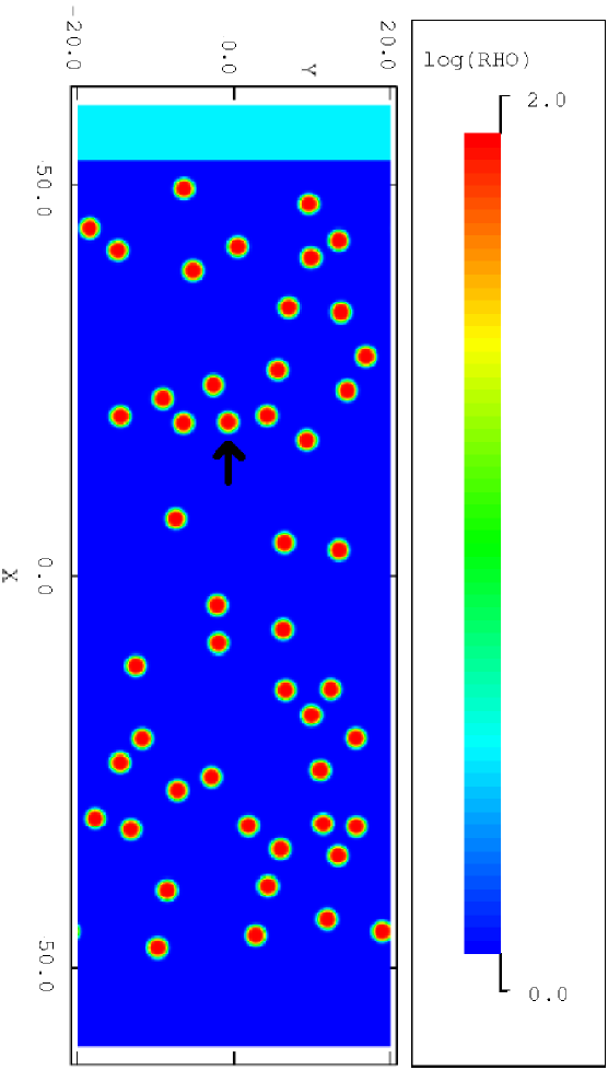
Figure 4: The initial ($t=0$) cloud distribution for a simulation of a shock overrunning multiple cylindrical clouds. The shock Mach number $M=3$, the cloud density contrast $\chi=10^{2}$, and the ratio of cloud mass to intercloud mass in the clumpy region is $MR=4$. The arrow marks an individual cloud for which the properties were monitored in time - see Fig. 6. In this plot and in all other density snapshots the spatial scale is in the units of the cloud radius and the density is in the units of the ambient density.

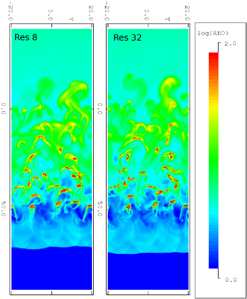
Figure 5: Resolution test for a Mach 3 shock overrunning multiple cylindrical clouds with the initial setup shown in Fig. 4. A logarithmic density plot is shown at $t=14.2\,t_{\rm cc}$ for resolutions of $R_{8}$ (left) and $R_{32}$ (right).

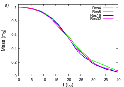
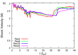
Figure 6: Resolution test for a Mach 3 shock overrunning multiple cylindrical clouds with $\chi=10^{2}$ and $MR=4$ (see Fig. 5). The time evolution of a) the total mass of all of the cloud cores, b) the mean shock velocity (normalized to the ambient intercloud sound speed) and c) the average core velocity of a single cloud, are shown.

2.2.2 Multiple clouds resolution test

We have also performed a convergence study for 2D multi-cloud simulations. In this study a Mach 3 shock overruns 48 identical cylindrical clouds, each with a density contrast to the intercloud medium of $\chi=10^{2}$. The ratio of cloud mass to intercloud mass within the clumpy region is $MR=4$. Fig. 4 shows the initial setup and distribution of clouds. The clouds fill a region which is $100\,r_{\rm cl}$ deep and $40\,r_{\rm cl}$ wide, with periodic boundaries in $y$. Resolutions of $R_{4}$, $R_{8}$, $R_{16}$ and $R_{32}$ were used. The latter required a grid with an effective size of $12800\times 1280$.

The shock exits the clumpy region at around $t=12.5\,t_{cc}$ in all of the simulations. Density plots for times just after this moment are shown in Fig. 5 for the $R_{8}$ and $R_{32}$ simulations. Higher compressions and greater fragmentation are seen in the higher resolution simulation. However, while significant differences in the behaviour of any individual cloud in the simulation can be identified, Fig. 6 shows that important global parameters in the multiple cloud simulation, such as the rate at which cloud mass is mixed into the flow (shown as the time evolution of the total mass of all of the cloud cores in Fig. 6a), the rate at which momentum is transferred from the flow to the clouds (shown as the velocity of a single cloud, Fig. 6c), and shock velocity (Fig. 6b) are not very sensitive to the resolution used.

Indeed, it is clear from Fig. 6 that a resolution of $R_{8}$ is sufficient in order to obtain an accurate representation of the global effect of multiple clouds on a flow. In previous multi-cloud simulations resolutions of $R_{32}$ and $R_{16}$ have been adopted (Poludnenko et al. (2002) and Poludnenko et al. (2004), respectively), but we show here that a somewhat lower resolution can be safely used, at least when a sub-grid turbulence model is employed. Therefore, we perform all other simulations in this work at a resolution of $R_{8}$.

3 Results

In this section we show the results of a number of simulations with different values of $M$, $\chi$, and $MR$. Table 1 summarizes the simulations that were performed. We adopt a naming convention such that m3chi2MR1 refers to a simulation with $M=3$, $\chi=10^{2}$ and $MR=1$.

Table 1: Summary of the multi-cloud simulations performed.

Simulation	$\chi$	$MR$	ncc	Shock Mach number
chi2MR0.25	$10^{2}$	0.25	128	3
chi2MR1	$10^{2}$	1	505	1.5, 3, 10
chi2MR1_double	$10^{2}$	1	1110	3
chi2MR4	$10^{2}$	4	1959	1.5, 2, 3, 10
chi3MR0.25	$10^{3}$	0.25	13	3
chi3MR1	$10^{3}$	1	51	3
chi3MR4	$10^{3}$	4	203	3

3.1 Mach 3 shock interactions

We first focus on simulations for a Mach 3 shock. Figs. 7 and 8 show the time evolution of the density distribution in simulation m3chi2MR4, which contains 1959 clouds. The shock sweeps through the clumpy region, propagating fastest through the channels between clouds. Behind the shock, the overrun clouds are in various stages of destruction, with the clouds closest to the shock being those which are in the earliest stage of interaction and which, therefore, are the most intact. Further behind the shock the clouds gradually lose their identities as they are mixed into the flow. Fig. 7 shows that a global bowshock moves upstream into the post-shock flow. Although the bowshock disappears out of view in Fig. 8, it remains on the grid which extends to $x=-450$. Low density (and pressure) regions in the post-shock flow are visible behind clouds as the flow rushes pass. The global shock front is momentarily deformed by each cloud that it encounters as it sweeps through the clumpy region. These local deformaties in the shock front gradually accumulate into a distortion of the shock front on larger length scales. The shock is most deformed as it reaches the end of the clumpy region (see the middle panel of Fig. 8). The other striking feature of the interaction is the formation of a dense shell in the post-shock flow due to the addition of mass from the destruction of the clouds. This is clearly seen in the panels in Fig. 8 and is the most important large-scale structure formed in the global flow as a result of the interaction.

The shock slows as it sweeps through the clumpy region and transfers momentum to cloud material. When the clumpy region is highly porous, the deceleration of the shock front is minimal and the clouds gradually reach the velocity of the postshock flow. This occurs if the global cloud cross section is small (for instance, when the mass ratio is low (e.g., $MR=0.25$) and/or when the cloud density contrast $\chi$ is high (e.g., $\chi=10^{3}$, $MR=1$ as in simulation m3chi3MR1).

Fig. 9 shows snapshots of the density distribution at the time that the shock exits the clumpy region in models m3chi2MR1 (top), m3chi2MR1_double (middle), and m3chi3MR4 (bottom). All of these models have lower number densities of clouds than model m3chi2MR4: in the first two models it is because the value of $MR$ is reduced, while in model m3chi3MR4 it is because the density contrast of the clouds has increased while the value of $MR$ is unchanged. As such, the clumpy region in each of these models is more porous than in model m3chi2MR4, and the shock is able to sweep through without such a significant reduction in its velocity. Comparison of Figs. 7, 8 and 9 also reveals significant differences between these models in the structures of the flow through the clumpy region.

Figure 7: The time evolution of the logarithmic density for model m3chi2MR4, shown at $t=0$ (top), $t=8.1\,t_{\rm cc}$ (middle) and $t=16.2\,t_{\rm cc}$ (bottom). The top panel also shows how the different cloud regions are defined.

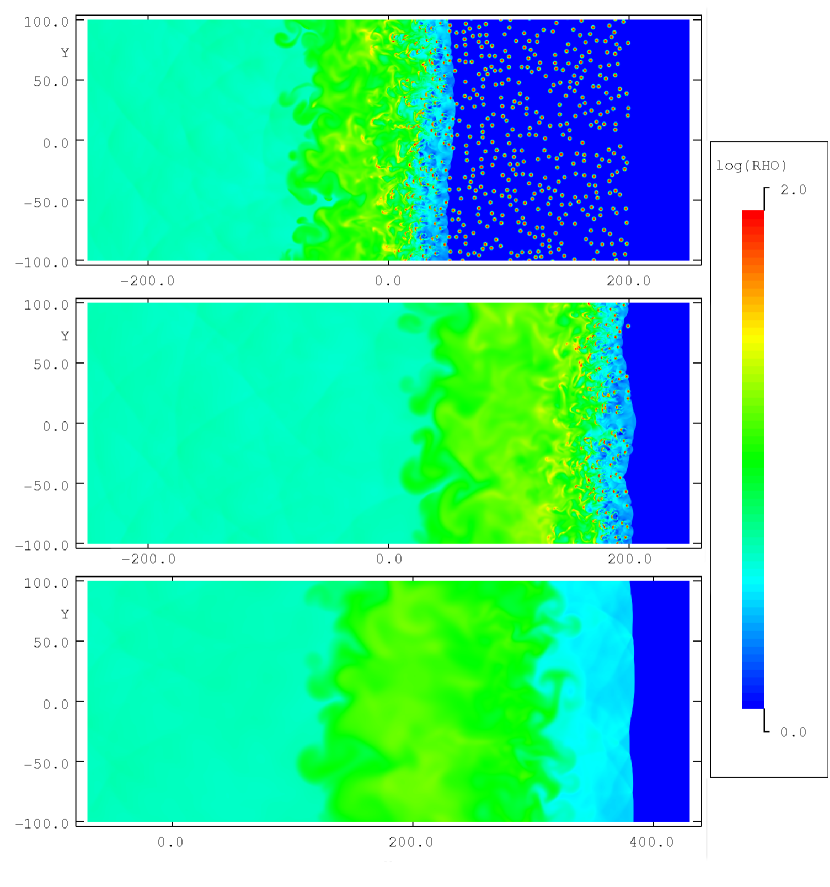
Figure 8: As Fig. 7 but at $t=36.6\,t_{\rm cc}$ (top), $t=61.0\,t{\rm cc}$ (middle) and $t=85.5\,t_{\rm cc}$ (bottom).

3.1.1 Velocity behaviour

As the shock sweeps through a clumpy region, it causes clouds in block 1 to accelerate first; then clouds in blocks 2, 3 and 4 accelerate. This transfer of momentum to the clouds inevitably causes the shock and the post-shock flow to slow. Figs. 10 and 11 show the time evolution of the average velocity of cloud material within particular blocks of clouds (e.g., as delineated in the top panel of Fig. 7) normalized to the intercloud sound speed.

Fig. 10 shows that the shock front slows down to about 50% of its initial velocity (though it remains supersonic). In this simulation we find that the first 3 blocks of clouds accelerate up to $1.25\,c_{1}$ (where $c_{1}$ is the sound speed in the intercloud ambient medium). However, by this point the post-shock flow immediately after the shock has decelerated to marginally below $1\,c_{1}$. Hence, material stripped from the upstream clouds pushes against the downstream clouds, compressing the clumpy region.

The shock front advances at roughly constant velocity after having reached a minimum while in the clumpy region. However, as the shock front leaves the clumpy region it reaccelerates at a roughly constant rate until it reaches a velocity somewhat smaller than the initial shock velocity. After that it accelerates very slowly, and asymptotically reaches its initial velocity (corresponding to Mach 3).

The final block of clouds is not held back by further clouds downstream and therefore does not stop accelerating at the same velocity as the other blocks. Instead it accelerates until it reaches the velocity of the post-shock flow after the shock stops reaccelerating. Blocks 3, 2 and 1 repeat this behaviour in that order.

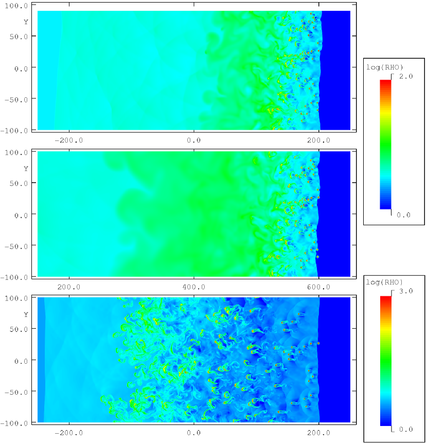
Figure 9: Snapshots of logarithmic density for models m3chi2MR1 (top), m3chi2MR1_double (middle), and m3chi3MR4 (bottom). The snapshots are taken as the shock front is exiting the cloudy region which occurs at $t=46\,t_{\rm cc}$, $t=95\,t_{\rm cc}$ and $t=13.5\,t_{\rm cc}$ respectively. Note the different colour scale of the bottom panel.

Figs. 11a) and b) show the velocities obtained in simulations m3chi2MR1 and m3chi2MR1_double, for which the mass ratio of cloud to intercloud material in the clumpy region is unity (the number density of clouds is therefore $4\times$ lower than in model m3chi2MR4). Model m3chi2MR1_double has a cloud distribution that is identical to that of model m3chi2MR1, but the distribution is repeated once to create a clumpy region that is twice as deep. In both cases the clumpy region is more porous and therefore, the reductions in the shock and post-shock velocities are not as severe as those seen in model m3chi2MR4. For this reason, the clouds are also accelerated initially to a higher velocity ($\approx 1.7c_{1}$) than in model m3chi2MR4.

As previously stated, the clumpy region can also be made more porous by increasing $\chi$ for a fixed $MR$. Fig. 11c) shows the velocity profiles obtained from model m3chi3MR4. As expected, the shock does not decelerate as much as in model m3chi2MR4. However, model m3chi3MR4 behaves differently in another way: because each cloud is more resistant to the flow, the clouds are not completely destroyed by the time the shock leaves the clumpy region (at $t\approx 13\,t_{\rm cc}$) when the collective cloud material from each block is still accelerating. In turn, due to continuing mass-loading of the flow, the shock continues to decelerate after it has left the clumpy region. In fact, the shock front decelerates until $t\approx 36\,t_{\rm cc}$, remains at constant velocity until $t\approx 44\,t_{\rm cc}$ and reaccelerates thereafter.

3.1.2 Stages of interaction

The behaviour of the simulations noted in the previous section allows the identification of 4 distinct phases in the evolution of the shock front. Firstly, there is a shock deceleration phase as the shock enters the clumpy region. This may be followed by a steady phase, when the shock front moves at constant velocity. The third stage is a reacceleration phase during which the shock front accelerates (at a fairly steady rate) into the homogeneous ambient medium. This stage always starts after the shock has traversed through the whole of the cloudy region, but not necessarily immediately after. The final stage begins once the shock’s acceleration slows. At this point the shock propagates with a velocity slightly slower than its initial velocity, but is continuing to accelerate very slowly, due to the constant velocity inflow trying to return the shock to its initial velocity.

The number and timings of the stages is model specific. In models for which the lifetime of the clouds is less than the crossing time of the shock through the clumpy region, the steady phase ends when the shock leaves the clumpy region (see, e.g., simulation m3chi2MR4 in Fig. 10). In models for which significant mass loading of the flow continues after the shock leaves the clumpy region the end of the steady phase is delayed (see, e.g., m3chi3MR4 in Fig. 11c).

The steady stage is best seen in models m3chi2MR4 and m3chi2MR1_double, and to some extent it is also visible in model m3chi3MR4. These are the simulations with the most mass in the clouds. Models chi2MR4 and chi3MR4 have the highest cloud to intercloud mass ratios of 4. In fact, the onset of a steady stage seems to intimately depend on the formation of a dense shell (see Sec. 3.1.3).

In contrast, model m3chi2MR1 (Fig. 11a) does not achieve a steady state. Instead the shock velocity evolves from the deceleration phase immediately into the reacceleration phase. One might expect that there is a better chance for a steady stage to occur if the clumpy region is deep. Fig. 11b indeed shows that a steady state occurs in model m3chi2MR1_double where the clumpy region is twice as deep as in model m3chi2MR1. The onset of the steady stage occurs when the shock is approximately halfway through the clumpy region, and all 4 stages can now be distinguished as in model m3chi2MR4.

For all of the $\chi=10^{2}$ models, the reacceleration stage begins the moment the shock leaves the clumpy region, but for the $\chi=10^{3}$ runs the onset of this stage shows more complicated behaviour. Because clouds with a higher density contrast evolve more slowly, significant evolution of the global flow can occur after the shock front leaves the clumpy region. Fig. 11c shows that this occurs in model m3chi3MR4, as the continued deceleration of the shock is evident. At some later time, presumably when the clouds are finally fully entrained into the flow, the shock starts to accelerate. There is also a hint of a steady stage in model m3chi3MR4, but examination of the velocity graphs reveals that it occurs at a much later evolutionary stage than in model m3chi2MR4 (as seen, e.g., when compared to the velocity evolution of material mixed in from the various blocks). Given that there are about $10\times$ fewer clouds in model m3chi3MR4 than in m3chi2MR4 this can be explained by the relative timescales involved in the shell formation which is discussed next.

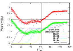
Figure 10: The time evolution of the mean $x$-velocity for cloud material for each different block in simulation m3chi2MR4. Also shown are the average velocity of the shock front and the velocity immediately behind the shock front. The vertical line indicates the time when the shock leaves the clumpy region, while the horizontal line indicates the initial speed of the post-shock flow.

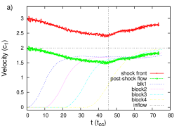
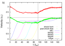
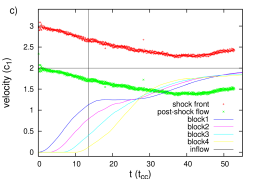
Figure 11: As Fig. 10 but for simulations a) m3chi2MR1, b) m3chi2MR1_double and c) m3chi3MR4.

3.1.3 Shell formation and evolution

Figs. 7 and 8 show that in model m3chi2MR4, a shell forms in the post-shock flow at $t=16.2\,t_{\rm cc}$. It is fully developed by $36.6\,t_{\rm cc}$. At $t=36.6\,t_{\rm cc}$ 7 distinct regions can be distinguished. A uniform ambient medium (without any clouds) lies at the right edge of the figure, while at the far left of the grid (off the figure in this case) lies the original post-shock flow specified by inflow boundary conditions at the upstream edge. A further 5 regions (from right to left) exist inbetween these other two. A region of unshocked clouds lies in the range $50\mathrel{\hbox to0.0pt{\lower 3.0pt\hbox{$\sim$}\hss}\raise 2.0pt\hbox{$<$}}x<200$. Shocked clouds embedded in a relatively low density postshock flow lie in the region $30\mathrel{\hbox to0.0pt{\lower 3.0pt\hbox{$\sim$}\hss}\raise 2.0pt\hbox{$<$}}x\mathrel{\hbox to0.0pt{\lower 3.0pt\hbox{$\sim$}\hss}\raise 2.0pt\hbox{$<$}}50$. Shocked clouds are being overrun by a denser shell in the region $-20\mathrel{\hbox to0.0pt{\lower 3.0pt\hbox{$\sim$}\hss}\raise 2.0pt\hbox{$<$}}x\mathrel{\hbox to0.0pt{\lower 3.0pt\hbox{$\sim$}\hss}\raise 2.0pt\hbox{$<$}}30$, though individual cores are still visible. This shell becomes gradually more uniform towards $x\approx-70$. The upstream edge of this dense shell is fairly distinct from the less dense gas that it abuts (at $x\approx-70$). The latter is gas in the original supersonic post-shock flow which has shocked against the clumpy region. This final region is bounded by a bow shock which lies off the left edge of the figure.

Fig. 12 shows the evolution of the density in the shell. Initially the average postshock density in the clumpy region is only about twice that of the shocked intercloud gas. However, as the clouds are destroyed and their mass mixes into the global flow, the density in this region increases. In model m3chi2MR4, a dense region, downstream of the region where distinct clouds are still visible, has formed by about the time that the shock reaches its minimum velocity. This is the “shell”. The compression of the shell progresses a little further, until a state in which the maximum density is steady in time is reached. This is reinforced by the simulation (model m3chi2MR1_double) for a wide clumpy region, which shows that the shell only becomes wider with time after this point. Once there are no more clouds blocking the path of the shell, it starts to expand from its leading edge, and the maximum density within it drops. This is seen clearly from Fig. 12, and is preceded by the shock reaching the edge of the clumpy region. Simulations with $\chi=10^{3}$ behave slightly differently - in these the density of the shell continues to increase after the shock has left the clumpy region due to the continued ablation of material from the longer-lived clouds.

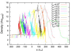
Figure 12: The density, volume averaged over $y$, as a function of $x$ in simulation M3chi2MR4, at different times. The shock exits the clumpy region at $t\approx 60\,t_{\rm cc}$.

3.1.4 Mach number profile

Fig. 13 shows the $y$-averaged Mach number profile of the flow in simulation M3chi2MR4 at $t=44.8\,t_{\rm cc}$. The undisturbed post-shock flow is mildly supersonic ($M\approx 1.04$), as seen at the far left of the panel. The shock at this time is just downstream of $x=100$.

In the region between $70\mathrel{\hbox to0.0pt{\lower 3.0pt\hbox{$\sim$}\hss}\raise 2.0pt\hbox{$<$}}x\mathrel{\hbox to0.0pt{\lower 3.0pt\hbox{$\sim$}\hss}\raise 2.0pt\hbox{$<$}}108$ clouds are overrun by the flow and accelerated by the gas streaming past, so that the Mach number of the flow increases as $x$ decreases. While the clouds remain identifiable as distinct entities, their interiors remain colder than the shocked intercloud flow, as initially the dense cloud is in pressure equilibrium with its less dense surroundings, so that its temperature is lower than that of the intercloud medium by a factor of $\chi$. Together these effects ensure that the Mach number of the flow eventually exceeds the Mach number in the undisturbed post-shock flow. The local Mach number reaches a peak of about 1.4, at a location corresponding to the downstream edge of the shell (which occupies a region between $-50\mathrel{\hbox to0.0pt{\lower 3.0pt\hbox{$\sim$}\hss}\raise 2.0pt\hbox{$<$}}x\mathrel{\hbox to0.0pt{\lower 3.0pt\hbox{$\sim$}\hss}\raise 2.0pt\hbox{$<$}}70$).

As the clouds begin to lose their individual identities their material is heated as it is mixed into the surrounding flow. This increases the sound speed of this material, and reduces the overall Mach number of the flow. The Mach number continues to decline with decreasing $x$ until the cloud material is fully mixed (which occurs at the upstream edge of the shell in this simulation). The region of constant Mach number ($M\approx 0.6$) between the upstream edge of the shell (at $x\approx-50$) and the bow shock at the head of the clumpy region (at $x\approx-265$) is the gas in the original post-shock flow which has shocked against the clumpy region.

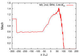
Figure 13: The local Mach number, volume averaged for all values of $y$, as a function of $x$ in simulation M3chi2MR4, at $t=44.8\,t_{\rm cc}$. The shock is at $x\approx 108$ and the bow shock is at $x\approx-265$.

3.2 Dependence on shock Mach number

Fig. 14 shows density snapshots when the shock front is exiting the clumpy region for models m1.5chi2MR4, m2chi2MR4 and m10chi2MR4. It is clear that a slower shock produces less compression, and that the shell which then forms is wider. In addition, weak shocks take longer to destroy clouds, so the shell forms further from the shock front. Perhaps most significantly, as the shock decelerates during its passage through the clumpy region it can slow so much that it decays into a wave which advances at the intercloud sound speed. This is seen in both the $M=1.5$ and $M=2$ simulations for which Fig. 14 reveals very weak density jumps at the edges of the clumpy regions.

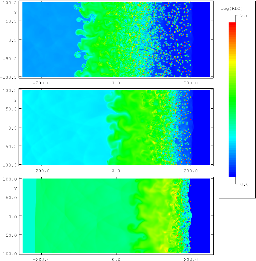
Figure 14: Snapshot of logarithmic density for models m1.5chi2MR4 (top), m2chi2MR4 (middle) and m10chi2MR4 (bottom). The snapshots are taken as the shock front is exiting the cloudy region which occurs at $t=53\,t_{\rm cc}$, $t=62\,t_{\rm cc}$ and $t=58\,t_{\rm cc}$ respectively. Relative to its initial speed, the $M=2$ shock is slowed the most.

Fig. 15 displays the $x$ component of the velocity averaged over all $y$ for the m1.5chi2MR4 and m2chi2MR4 simulations normalized to the ambient intercloud sound speed. The points show the velocity of the shock calculated by an algorithm which searches for a pressure jump. However, when the shock decays into a wave the pressure jump largely disappears and this calculation fails. The points with error bars then show the velocity of the disturbance determined by measuring, by eye, the position of the leading edge of the disturbance. In the $M=2$ simulation the average velocity of the shock/wave disturbance is close to transonic. Close examination reveals that the shock appears fragmented and local regions of sonic waves can be seen. The shock completely decays into a sonic wave in the $M=1.5$ simulation. These results are in harmony with theoretical predictions based on a uniform density region suggesting that a supersonic to subsonic transition occurs at this mass ratio if the initial shock Mach number is $M\sim 2$ (see Sec. 3.3 for further details).

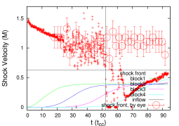
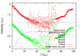
Figure 15: The time evolution of the $x$ component of the velocity averaged over all values of $y$, for different regions in simulations m1.5chi2MR4 (top) and m2chi2MR4 (bottom). Also shown are the average shock front velocities. The shock velocity varies when parts of the shock front become subsonic. Vertical lines indicate the time when the shock leaves the clumpy region.

3.3 The reduction in the shock speed

Fig. 16 shows the minimum shock speed (normalized to the initial shock speed) as a function of shock Mach number obtained in simulations with $MR=4$ and $\chi=10^{2}$ (plotted as black crosses). The minimum shock speed in each case occurs during a “steady” stage when the shock is moving through the clumpy region. The error bars correspond to the $1\sigma$ spread in measured speeds. We have already noted that in the $M=1.5$ simulation the shock slows to the point that the disturbance becomes a wave. In this case the minimum speed is limited by the sound speed in the intercloud medium, as seen in Fig. 16. The situation in the $M=2$ simulation is not so straightforward - a global shock front is visible but there are local regions where a wave is seen instead.

We can compare the measured shock speed to the expected speed of a shock transmitted into a region of enhanced density. For this we make use of eq. 5.4 in Klein et al. (1994), for a shock interacting with a single cloud:

$$v_{\rm s}=(F_{\rm st}F_{\rm c1})^{1/2}\chi^{-1/2}v_{0}.$$ (1)

Here $F_{\rm st}\equiv P_{3}/P_{1}$, where $P_{1}$ is the pressure far upstream and $P_{3}$ is the stagnation pressure (just upstream of the cloud), and $F_{\rm c1}\equiv P_{4}/P_{3}$ is the ratio of the pressure just behind the transmitted shock and the stagnation pressure. In the limit of high Mach number and high density contrast,

$$F_{\rm st}\simeq 1+\frac{2.16}{1+6.55\chi^{-1/2}}.$$ (2)

To apply this expression to our multi-clump simulations we need an “effective” value for $\chi$ which accounts for the inhomogeneity of the clumpy region. We choose this value to be $\chi_{\rm eff}=MR+1$, which is the average density contrast of the region (total mass of the region divided by the mass a same size region of ambient density would have). Furthermore, in simulations where the clumpy region is replaced with a region of uniform density (see Sec. 3.4), it is clear that $P_{4}=P_{3}=P_{2}$, where $P_{2}$ is the pressure just after the bow shock. We shall assume that this is also the case for our multiple cloud simulations, and therefore adopt $F_{\rm c1}=1$. For our clumpy simulations with $MR=4$ and $\chi=10^{2}$ we therefore obtain $\chi_{\rm eff}=5$ and $F_{\rm st}=1.55$, so that Eq. 1 gives $v_{\rm s}=0.56v_{0}$. As can be seen, this is comparable to the values shown in Fig. 16, in which the $v_{s}=0.56v_{0}$ line is plotted.

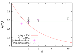
Figure 16: The reduction in shock speed (black crosses, as measured during the “steady” phase as the shock propagates through the clumpy region) normalized to the initial shock speed. The reduction is plotted as a function of the initial shock Mach number, $M$, for simulations with $\chi=10^{2}$ and $MR=4$. Also shown is the equivalent reduction in speed of a shock propagating through a uniform density enhancement (pink crosses - see Sec. 3.4).

3.4 Comparisons to a shock encountering a region of uniform density

In the limit of an infinitely deep/thick cloud distribution we expect the global behaviour of the shock to approach that of a shock encountering a uniform medium of the same average density. This could be similar to the steady state reached in some of our simulations. Therefore, we have performed a number of additional calculations of a shock encountering a uniform region of enhanced density equal to the average density of a clumpy region with $MR=4$. The minimum shock speed through this region is shown in Fig. 16 with pink crosses. As can be seen, the agreement with the multi-cloud simulations is very good, with significant deviation only at $M=1.5$. Clearly the minimum shock speed obtained in our multi-cloud simulations is close to the shock speed occuring in a comparable region of uniform density.

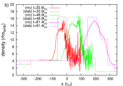
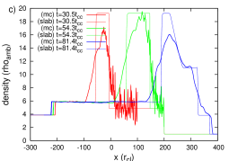
Figure 17: Snapshots of the $x$-dependance of the density averaged over all values of $y$ (thick lines) from simulations a) m2chi2MR4, b) m3chi2MR4 and c) m10chi2MR4. Also shown are density profiles from simulations with uniform but corresponding density. In all cases the shock exits the region of enhanced density (smooth or clumpy) at $t\approx 60\,t_{\rm cc}$.

Fig. 17 compares the $x$-dependance of the density, averaged over all values of $y$, given by simulations of a shock interacting with a uniform region of enhanced density to analogous profiles obtained from our multiple cloud simulations. One notices the similarity between the profiles: the maximum density of the shell and the reduction in density after the shock exits the higher density/clumpy region are similar. Obviously, the uniform region simulations yield distinct edges and slopes corresponding to the shocks and rarefaction waves, whereas the multiple cloud simulations give smoother profiles. The smoothing length is of the order of $L_{\rm CD}$, which is the distance that a cloud is displaced by the flow prior to its destruction (Poludnenko et al. 2002). For the same reason the width of the densest part of the shell is narrower in the multiple cloud simulations.

The picture of a shock transmitted into a uniform density region is different. The velocity jumps according to Rankine-Hugoniot conditions. As the shock front is moving faster than the postshock flow, the width, $w$ of the compressed region is increasing at a rate given by:

$$\frac{dw}{dt}=v_{s}-v_{ps}=\left(\frac{3}{4M_{u}}+\frac{M_{u}}{4}\right)c_{u}.$$ (3)

where $M_{u}$ is the Mach number of a shock transmitted into a uniform medium and $c_{u}$ is the sound speed in that medium. Eqs. 1 and 2 can be used to determine $M_{u}$, but the approximation in Eq. 2 is only valid at high Mach numbers and high density contrasts. However, we can obtain an estimate based on Eq. 1. As $F_{st}\geq 1$ and, because the shock is steady, $F_{c}=1$ (Klein et al. 1994), $M_{u}\geq M_{0}$ and so $\frac{dw}{dt}\geq\frac{M_{0}c_{1}}{4}$. Furthermore, two limiting cases can be found. In the limit of a weak shock $\frac{dw}{dt}\approx c_{u}$; this is the minimum value, and it would be higher in all other cases. In the limit of a strong shock and high $\chi$, $\frac{dw}{dt}\approx 0.44M_{0}c_{u}$.

Fig. 17 shows that the widths of shells in clumpy regions correspond well to those in regions of equivalent uniform density. As such Eq. 3 can be used, with $M_{u}$ either determined from a corresponding uniform density case, or by replacing it with $v_{s}/c_{u}$, with $c_{u}$ determined for the medium of corresponding uniform density. The limiting cases would be different though. In the weak shock limit, the shock may decay into a sound wave. In such a case $\frac{dw}{dt}\approx c_{1}$, but it could be significantly less depending on how this affects individual cloud lifetimes. In the limit of very high $\chi$ the upstream edge of the shell takes a long time to reach $v_{ps}$ and is effectively stationary, so $\frac{dw}{du}=v_{s}$.

3.5 Individual cloud evolution

We expect individual clouds to evolve differently when overrun by a mass-loaded evolved shock which has been altered by the presence of clouds further upstream than when they are overrun by a steady planar shock. Section 3.1.1 shows that the shock Mach number and in turn the velocity of the post shock flow decreases as the shock sweeps up cloud material. The lower velocity of the shock should prolong the lifetime of a cloud, but this may be offset by the increased density of the flow. Furthermore, the postshock flow is much more turbulent. This aids the development of cloud-destroying instabilities (see Pittard et al. 2009). Finally, a region of higher density follows some distance behind the shock. In the extreme case it is a dense shell, but even if a shell does not fully form, remnants of upstream clouds may well interact with clouds further downstream. Therefore, it is difficult to predict whether downstream clouds are destroyed more readily than their upstream counterparts. However, we can use our simulation results to investigate this.

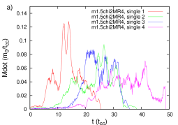
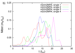
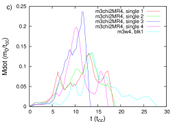
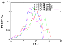
Figure 18: Normalized mass loss rates for select individual clouds in simulations chi2MR4 for different Mach numbers: a) $M=1.5$, b) $M=2$, c) $M=3$ and d) $M=10$.

Mass loss rates from different clouds in the simulations are shown in Fig. 18. Each cloud is from a particular block (see, e.g., Fig. 7), and the time in each plot has been shifted so that $t=0$ corresponds to the time when the shock first encounters the cloud under consideration. The greatest differences between the evolution of different clouds in a given simulation occur in model m1.5chi2MR4, as shown in Fig. 18a). Here the cloud in the block which is first to be hit by the shock (labelled single1) encounters a flow which is relatively unmodified by the small number of clouds which lie further upstream. Although the interaction is relatively weak because of the modest shock Mach number, significant mass-loss from the cloud occurs after $t=\,5t_{\rm cc}$, and the core of the cloud is completely destroyed by $t\approx 27\,t_{\rm cc}$ (a similar lifetime occurs for spherical clouds - see Pittard et al. 2010). In contrast, significant mass-loss does not occur until $t\approx 10\,t_{\rm cc}$ for the cloud in the second block (labelled single2), and until $t\approx 12\,t_{\rm cc}$ and $13\,t_{\rm cc}$ for clouds in the third and fourth blocks (labelled single3 and single4, respectively). The low initial mass-loss rates from clouds further downstream is due to the decay of the shock into a wave as it moves through the clumpy medium. While the flow past the cloud is subsonic the mass-loss rate remains very low.

The same initial behaviour is also seen in simulation m2chi2MR4, as shown in Fig. 18b). In contrast, at higher shock Mach numbers (models m3chi2MR4 and m10chi2MR4 in Fig. 18) the shock remains supersonic as it transits through the clumpy region, and differences between the clouds in the evolution of their mass-loss rates are not so readily apparent (see Fig. 18c and d).

It is clear that the cloud lifetimes must be compared in a statistical way. Fig. 19 shows the ratio of the lifetimes of individual clouds to the lifetime of the equivalent cloud hit by a “clean” shock (i.e. initially with no post-shock structure due to interactions with upstream clouds), $R_{\rm life}$. The top panel in Fig. 19 shows the results for $M=3$, while the bottom panel shows the results for $M=10$. In both cases there is a general trend for a reduction in $R_{\rm life}$ with increasing $MR$, albeit with a reasonably large scatter for a particular cloud. Table 2 notes the average value of $R_{\rm life}$ in a given simulation, where this trend is now even clearer. When $MR=4$, we find that downstream clouds have lives which are about 40% shorter than the lifetime of an isolated. Table 2 also indicates that there is no clear trend of $R_{\rm life}$ with the shock Mach number $M$ for a given value of the mass-ratio, $MR$. Finally, a simulation performed at twice our standard resolution reveals that there is currently a slight resolution dependence on $R_{\rm life}$ (model m3chi2MR4 returns $R_{\rm life}=0.62\pm{0.07}$ and $0.72\pm{0.02}$ at a resolution of 8 and 16 cells per cloud radius, respectively).

The reduction in the cloud lifetime due to the turbulent nature of the flow is clearly more significant than the weakening and broadening of the shock which acts to increase the cloud lifetime (Williams & Dyson 2002).

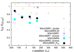
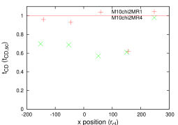
Figure 19: Ratio of the lifetime of a downstream cloud to the equivalent lifetime obtained when the cloud is hit by a “clean” shock with a uniform post-shock flow.

Table 2: Ratio of the lifetimes of a downstream cloud to the equivalent lifetime of an “isolated” cloud. The quoted ratio is averaged over the lifetime of the individual cloud tracked in each block of clouds.

Simulation	$R_{\rm life}$
m2chi2MR4	$0.55\pm{0.07}$
m3chi2MR0.25	$0.92\pm{0.07}$
m3chi2MR1	$0.83\pm{0.14}$
m3chi2MR4	$0.62\pm{0.07}$
m3chi2MR4_R16	$0.72\pm{0.02}$
m10chi2MR1	$0.86\pm{0.22}$
m10chi2MR4	$0.62\pm{0.06}$

4 Discussion

Our work is relevant to objects where hot, diffuse gas interacts with a colder dense phase. In many of these objects the cold phase, despite its low volume filling fraction, may dominate the dynamics of the hot phase, and thus significantly change the morphology and evolution of the object, and its emission. On the smallest scales these objects include wind-blown bubbles and supernova remnants. Cowie et al. (1981) were the first to study the behaviour of supernova remnants expanding into a clumpy medium. They found that the destruction of the clouds leads to the highest densities in the remnant occuring over the outer half radius (in contrast, when there is no mass loading, a thin dense shell forms at the forward shock). These findings have since been supported by Dyson & Hartquist (1987), who reported a similar ”thick shell” morphology in their similarity solutions, and by the additional numerical simulations presented by Dyson et al. (2002) and Pittard et al. (2003). The X-ray emission in these cases becomes softer and more extended. In other work, Arthur & Henney (1996) studied the effects of mass loading by hydrodynamic ablation on supernova remnants evolving inside cavities evacuated by the stellar winds of the progenitor stars. They showed that the extra mass injected by embedded clumps was capable of producing the excess soft X-ray emission seen in some bubbles in the Large Magellanic Cloud. We conclude, therefore, that cloud destruction by ablation, as in the simulations presented in our paper, can be looked for by searching for its affect on the X-ray emission of supernova remnants.

The interaction between a wind and individual clouds is also seen in observations of planetary nebula. For instance, in NGC 7293 (the Helix nebula) long molecular tails and bright cresent-rimmed clouds are spectacularly resolved (O’Dell et al. 2005; Hora et al. 2006; Matsuura et al. 2007). The tails in the outer part of the nebula are less clear due to projection effects, but appear to be a separate population displaying wider opening angles. This may reflect changes in the diffuse flow past the clouds, possibly due to the material stripped off the clouds further upstream. Observations indicate that the flow past the clouds is mildly supersonic. Although numerical simulations are able to match the basic morphology of the tails (Dyson et al. 2006), dedicated 3D simulations of clouds with very high density contrasts to the ambient flow are required in order for further insight to be gained.

On larger scales, we note that there is substantial support for mass-loading in starburst regions. Broad emission-line wings are seen in many young star forming regions including 30 Doradus (Chu & Kennicutt 1994; Melnick et al. 1999), NGC 604 (Yang et al. 1996), and NGC 2363 (Roy et al. 1992; Gonzalez-Delgado et al. 1994), and more distant dwarf galaxies (e.g. Marlowe et al. 1995; Izotov et al. 1996; Homeier & Gallagher 1999; Sidoli et al. 2006). More recently, Westmoquette et al. (2007a, b) reported on the broad emission-line component in the dwarf irregular starburst galaxy NGC 1569. Although the nature of the broad lines has yet to be fully determined, evidence is mounting that it is associated with the impact of cluster winds on cool gas knots. It therefore traces both mass-loading of wind material and mass entrainment. Further support for mass-loading comes from the analysis of hard X-ray line emission within starburst regions. Strickland & Heckman (2009) determine that as much material is mass-loaded into the central starburst region of M82 as is expelled by the winds and supernovae which pressurize the region. A key future goal is the development of numerical simulations of the multi-phase gas within starburst regions, and predictions for broad emission-line wings and X-ray emission.

Starbursts are often associated with galactic outflows. These flows are observed to be filamentary. The consensus view is that the clumps at the heads of the filaments are material which is ripped out of the galactic disk as the galactic wind develops (i.e. representing additional, distributed, mass-loading). In some cases the filaments appear to be confined to the edges of the outflow (Shopbell & Bland-Hawthorn 1998), while in other objects they appear to fill the interior of the wind (Veilleux & Bland-Hawthorn 1997). It is clear that material stripped from the H$\alpha$ emitting clouds is entrained into the outflow (see, e.g. Cooper et al. 2008), but the exact amount is notoriously difficult to measure (Veilleux et al. 2005). Again, future dedicated simulations are needed to help address this issue.

A key question concerns the ultimate fate of gas within galactic outflows. Observations and simulations indicate that the majority of the energy in galactic winds is in the kinetic energy of the hot gas, while the mass in the outflow is dominated by the warm photoionized gas. The former has a good chance of escaping the gravitational potential of the host galaxy, while the latter in many cases is unlikely to do so. Even when simple energetic arguments suggest that the ISM can be completely expelled from a starbursting galaxy, whether it will actually occur depends strongly on the geometry and multiphase nature of the ISM (see, e.g., Heckman et al. 1995). For instance, if a centrally concentrated starburst occurs in a galaxy with a disk-like ISM, blowout of the superbubble along the minor axis can allow the bulk of the ISM in the disk to be retained by the galaxy. With a multiphase ISM the diffuse intercloud medium may be ejected while large dense clouds remain in the disk.

Recent work by Oppenheimer & Davé (2008) indicates that the range of galactic winds is primarily determined by the interaction of the wind with the ambient environment, with the gravity of the parent galaxy playing a less significant role. Their simulations also show that across cosmic time the average wind particle has participated in a wind several times. However, further investigations are needed, since their simulations currently lack the resolution required to make accurate quantitative predictions of the slowing of the winds and wind recycling. Furthermore, the wind’s multiphase nature must be addressed. Studies like ours are relevant to this work since the destruction and acceleration timescales which we find for our clumpy region have some bearing on the mixing and stalling timescales of a galactic wind. Such simulations could be tested against observations of the extent of galactic winds (e.g. Tumlinson et al. 2011; Tripp et al. 2011).

5 Conclusions

We have performed a detailed investigation of a shock running through a clumpy region. We find the following key behaviour:

• The stripping of material from the clouds “mass-loads” the post-shock flow and leads to the formation of a dense shell. Fully-mixed material within the shell reaches a maximum density, after which the shell grows in width. The shell expands and its density drops once there are no more clouds to mix in.

• The evolution of the shock can be split into several distinct stages. During the first stage, the shock decelerates. Then in some cases its velocity becomes nearly constant. After deceleration and the constant speed phase, if it occurs, the shock accelerates and finally approaches the speed it had in the uniform medium before it encountered the clumpy region. A steady stage does not always occur (e.g., if the clumpy region is not very deep).

• When the mass-loading is sufficient, the flow can be slowed to the point that the shock degenerates into a wave.

• The clumpy region becomes more porous as the number density of clouds is reduced, which occurs for lower values of $MR$, and/or increased values of $\chi$.

• A great deal of turbulence is generated in the post-shock flow as it sweeps through the clumpy region. Clouds exposed to this turbulence can be destroyed in only 60% of the time needed to destroy a similar cloud in an “isolated” environment. The lifetime of downstream clouds decreases with increasing $MR$.

We have determined the necessary conditions (in terms of the cloud density contrast and the ratio of cloud mass to intercloud mass) for a clumpy region to have a significant effect on a diffuse flow. The lifetime of clouds is a key factor in this respect. Pittard et al. (2009) first showed that clouds can be destroyed more quickly when overrun by a highly turbulent environment, although the strength of this turbulence was treated as a free parameter. In contrast, in this paper we have presented the first self-consistent simulations of a highly turbulent flow overrunning clouds, where the enhanced turbulence is a natural consequence of the flow overruning clouds further upstream. Since our simulations are purely hydrodynamic, the next step will be to investigate the effects of magnetic fields and thermal conduction on the flow dynamics. In future papers we will also investigate the ability of a flow to force its way through a finite-sized clumpy medium, and determine how this depends on the ratio of the mass injection rate from the clouds to the mass flux in the wind.

References

- Arthur & Henney (1996) Arthur, S. J., & Henney, W. J. 1996, ApJ, 457, 752
- Chu & Kennicutt (1994) Chu, Y.-H., & Kennicutt, Jr., R. C. 1994, ApJ, 425, 720
- Cooper et al. (2008) Cooper, J. L., Bicknell, G. V., Sutherland, R. S., & Bland-Hawthorn, J. 2008, ApJ, 674, 157
- Cowie et al. (1981) Cowie, L. L., McKee, C. F., & Ostriker, J. P. 1981, ApJ, 247, 908
- Dyson et al. (2002) Dyson, J. E., Arthur, S. J., & Hartquist, T. W. 2002, A&A, 390, 1063
- Dyson & Hartquist (1987) Dyson, J. E., & Hartquist, T. W. 1987, MNRAS, 228, 453
- Dyson et al. (2006) Dyson, J. E., Pittard, J. M., Meaburn, J., & Falle, S. A. E. G. 2006, A&A, 457, 561
- Einfeldt (1988) Einfeldt, B. 1988, SIAM Journal on Numerical Analysis, 25, 294
- Falle (1994) Falle, S. A. E. G. 1994, MNRAS, 269, 607
- Gonzalez-Delgado et al. (1994) Gonzalez-Delgado, R. M., Perez, E., Tenorio-Tagle, G., et al. 1994, ApJ, 437, 239
- Heckman et al. (1995) Heckman, T. M., Dahlem, M., Lehnert, M. D., et al. 1995, ApJ, 448, 98
- Homeier & Gallagher (1999) Homeier, N. L., & Gallagher, J. S. 1999, ApJ, 522, 199
- Hora et al. (2006) Hora, J. L., Latter, W. B., Smith, H. A., & Marengo, M. 2006, ApJ, 652, 426
- Izotov et al. (1996) Izotov, Y. I., Dyak, A. B., Chaffee, F. H., et al. 1996, ApJ, 458, 524
- Jun et al. (1996) Jun, B.-I., Jones, T. W., & Norman, M. L. 1996, ApJL, 468, L59
- Klein et al. (1994) Klein, R. I., McKee, C. F., & Colella, P. 1994, ApJ, 420, 213
- Marlowe et al. (1995) Marlowe, A. T., Heckman, T. M., Wyse, R. F. G., & Schommer, R. 1995, ApJ, 438, 563
- Matsuura et al. (2007) Matsuura, M., Speck, A. K., Smith, M. D., et al. 2007, MNRAS, 382, 1447
- McKee & Ostriker (1977) McKee, C. F., & Ostriker, J. P. 1977, ApJ, 218, 148
- Melnick et al. (1999) Melnick, J., Tenorio-Tagle, G., & Terlevich, R. 1999, MNRAS, 302, 677
- Nakamura et al. (2006) Nakamura, F., McKee, C. F., Klein, R. I., & Fisher, R. T. 2006, ApJS, 164, 477
- Nessyahu & Tadmor (1990) Nessyahu, H., & Tadmor, E. 1990, Journal of Computational Physics, 87, 408
- O’Dell et al. (2005) O’Dell, C. R., Henney, W. J., & Ferland, G. J. 2005, ApJ, 130, 172
- Oppenheimer & Davé (2008) Oppenheimer, B. D., & Davé, R. 2008, MNRAS, 387, 577
- Orlando et al. (2008) Orlando, S., Bocchino, F., Reale, F., Peres, G., & Pagano, P. 2008, ApJ, 678, 274
- Pittard et al. (2003) Pittard, J. M., Arthur, S. J., Dyson, J. E., et al. 2003, A&A, 401, 1027
- Pittard et al. (2005) Pittard, J. M., Dyson, J. E., Falle, S. A. E. G., & Hartquist, T. W. 2005, MNRAS, 361, 1077
- Pittard et al. (2009) Pittard, J. M., Falle, S. A. E. G., Hartquist, T. W., & Dyson, J. E. 2009, MNRAS, 394, 1351, p09
- Pittard et al. (2010) Pittard, J. M., Hartquist, T. W., & Falle, S. A. E. G. 2010, MNRAS, 405, 821
- Poludnenko et al. (2002) Poludnenko, A. Y., Frank, A., & Blackman, E. G. 2002, ApJ, 576, 832
- Poludnenko et al. (2004) Poludnenko, A. Y., Dannenberg, K. K., Drake, R. P., et al. 2004, ApJ, 604, 213
- Roy et al. (1992) Roy, J.-R., Aube, M., McCall, M. L., & Dufour, R. J. 1992, ApJ, 386, 498
- Sales et al. (2010) Sales, L. V., Navarro, J. F., Schaye, J., et al. 2010, MNRAS, 409, 1541
- Shopbell & Bland-Hawthorn (1998) Shopbell, P. L., & Bland-Hawthorn, J. 1998, ApJ, 493, 129
- Sidoli et al. (2006) Sidoli, F., Smith, L. J., & Crowther, P. A. 2006, MNRAS, 370, 799
- Steffen et al. (1997) Steffen, W., Gomez, J. L., Raga, A. C., & Williams, R. J. R. 1997, ApJL, 491, L73
- Strickland & Heckman (2009) Strickland, D. K., & Heckman, T. M. 2009, ApJ, 697, 2030
- Tripp et al. (2011) Tripp, T. M., Meiring, J. D., Prochaska, J. X., et al. 2011, Science, 334, 952
- Tumlinson et al. (2011) Tumlinson, J., Thom, C., Werk, J. K., et al. 2011, Science, 334, 948
- Veilleux & Bland-Hawthorn (1997) Veilleux, S., & Bland-Hawthorn, J. 1997, ApJL, 479, L105
- Veilleux et al. (2005) Veilleux, S., Cecil, G., & Bland-Hawthorn, J. 2005, ARA&A, 43, 769
- Westmoquette et al. (2007a) Westmoquette, M. S., Exter, K. M., Smith, L. J., & Gallagher, J. S. 2007a, MNRAS, 381, 894
- Westmoquette et al. (2007b) Westmoquette, M. S., Smith, L. J., Gallagher, J. S., & Exter, K. M. 2007b, MNRAS, 381, 913
- Williams & Dyson (2002) Williams, R. J. R., & Dyson, J. E. 2002, MNRAS, 333, 1
- Yang et al. (1996) Yang, H., Chu, Y.-H., Skillman, E. D., & Terlevich, R. 1996, ApJ, 112, 146
- Yirak et al. (2010) Yirak, K., Frank, A., & Cunningham, A. J. 2010, ApJ, 722, 412