Ab-initio angle and energy resolved photoelectron spectroscopy with time-dependent density-functional theory

Abstract

We present a time-dependent density-functional method able to describe the photoelectron spectrum of atoms and molecules when excited by laser pulses. This computationally feasible scheme is based on a geometrical partitioning that efficiently gives access to photoelectron spectroscopy in time-dependent density-functional calculations. By using a geometrical approach, we provide a simple description of momentum-resolved photoemission including multi-photon effects. The approach is validated by comparison with results in the literature and exact calculations. Furthermore, we present numerical photoelectron angular distributions for randomly oriented nitrogen molecules in a short near infrared intense laser pulse and helium-(I) angular spectra for aligned carbon monoxide and benzene.

I Introduction

Photoelectron spectroscopy is a widely used technique to analyze the electronic structure of complex systems Ellis et al. (2005); Wu et al. (2011). The advent of intense ultra-short laser sources has extended the range of applicability of this technique to a vast variety of non-linear phenomena like high-harmonic generation, above-threshold ionization (ATI), bond softening and vibrational population trapping Brabec and Krausz (2000). Furthermore, it turned attosecond time-resolved pump-probe photoelectron spectroscopy into a powerful technique for the characterization of excited-states dynamics in nano-structures and biological systems Krausz (2009). Angular-resolved ultraviolet photoelectron spectroscopy is by now established as a powerful technique for studying geometrical and electronic properties of organic thin films Puschnig et al. (2009); Kera et al. (2006). Time-resolved information from streaking spectrograms Schultze et al. (2010), shearing interferograms Remetter et al. (2006), photoelectron diffraction Meckel et al. (2008), photoelectron holography Huismans et al. (2011), etc. hold the promise of wavefunction reconstruction together with the ability to follow the ultrafast dynamics of electronic wave-packets. Clearly, to complement all these experimental advances, and to help to interpret and understand the wealth of new data, there is the need for ab-initio theories able to provide (time-resolved) photoelectron spectra (PES) and photoelectron angular distributions (PAD) for increasingly complex atomic and molecular systems subject to arbitrary perturbations (laser intensity and shape).

Photoelectron spectroscopy is a general term which refers to all experimental techniques based on the photoelectric effect. In photoemission experiments a light beam is focused on a sample, transferring energy to the electrons. For low light intensities an electron can absorb a single photon and escape from the sample with a maximum kinetic energy $\hbar\omega-I_{P}$ (where $\omega$ is the photon angular frequency and $I_{P}$ the first ionization potential of the system) while for high intensities electron dynamics can be interpreted considering a three-step model Corkum (1993). This model provides a semiclassical picture in terms of ionization followed by free electron propagation in the laser field with return to the parent ion, and rescattering. Such rescattering processes are the source of many interesting physical phenomena. In the case of long pulses, for instance, multiple photons can be absorbed resulting in emerging kinetic energies of $s\hbar\omega-I_{P}-U_{P}$ (where $s$ is the number of photons absorbed, $U_{P}=\epsilon^{2}/4\omega^{2}$ is the ponderomotive energy and $\epsilon$ the electric field amplitude) forming the so called ATI peaks in the resulting photoelectron spectrum. In all cases the observable is the escaping electron momentum measured at the detector.

In general, the interaction between electrons in an atom or molecule and a laser field is difficult to treat theoretically, and several approximations are usually performed. Clearly, a full many-body description of PES is prohibitive, except for the case of few (one or two) electron systems Lein et al. (2001); Pazourek et al. (2012); Ishikawa and Ueda (2012). As a consequence, the direct solution of the time dependent Schrödinger equation (TDSE) in the so-called single-active electron (SAE) approximation is a standard investigation tool for many strong-field effects in atoms and dimers and represents the benchmark for analytic and semi-analytic models Schafer and Kulander (1990); Chelkowski et al. (1998); Grobe et al. (1999); Chen et al. (2006); Tong et al. (2006, 2007); Awasthi et al. (2008); Petretti et al. (2010); Schultze et al. (2010); Burenkov et al. (2010); Huismans et al. (2011); Zhou and Chu (2011); Tao and Scrinzi (2012); Catoire and Bachau (2012). Perturbative approaches based on the standard Fermi golden rule are usually employed. For weak lasers, plane wave methods Puschnig et al. (2009) and the independent atomic center approximation Grobman (1978) have been applied, while in the strong field regime, Floquet theory, the strong-field approximation Huismans et al. (2011); Gazibegović-Busuladžić et al. (2011) and semiclassical methods Corkum (1993); Lewenstein et al. (1995); Paulus et al. (1999) are routinely used.

From a numerical point of view, it would be highly desirable to have a PES theory based on time-dependent density functional theory (TDDFT) Runge and Gross (1984); Marques et al. (2011) where the complex many-body problem is described in terms of a fictitious single-electron system. For a given initial many body state, TDDFT maps the whole many-body problem into the time dependence of the density from which all physical properties can be obtained. The method is in principle exact, but in practice approximations have to be made for the unknown exchange-correlation functional as well as for specific density-functionals providing physical observables. This latter issue is much less studied than the former, and to the best of our knowledge a formal derivation of momentum-resolved PES from the time dependent density has not been performed up to now. In any case, several works were published addressing the problem of single and multiple ionization processes within TDDFT. For example, ionization rates were calculated for atoms and molecules Chu and Chu (2004); Telnov and Chu (2009a); Son and Chu (2009a, b); Hansen et al. (2011), and TDDFT with the sampling point method (SPM) has been employed in the study of PES and PAD for sodium clusters Pohl et al. (2000, 2004); Wopperer et al. (2010a, b).

In this work, besides presenting a formal derivation of a photoelectron orbital functional, we report on a new and physically sound scheme to compute PES of interacting electronic systems in terms of the time-dependent single electron Kohn-Sham (KS) wavefunctions. The scheme relies on geometrical considerations and is based on a splitting technique Chelkowski et al. (1998); Grobe et al. (1999); Chen et al. (2006); Tong et al. (2006, 2007). The idea is based on the of partitioning of space in two regions (see Fig. 1 below): In the inner region, the KS wave function is obtained by solving the TDDFT equations numerically; in the outer region, electrons are considered as free particles, the Coulomb interaction is neglected, and the wavefunction is propagated analytically with only the laser field. Electrons flowing from the inner region to the outer region are recorded and coherently summed up to give the final result. In addition to the adaptation of the traditional splitting procedure to TDDFT, we propose a novel scheme where electrons can seamlessly drift from one region to the other and spurious reflections are greatly suppressed. This procedure allows us to reduce considerably the spatial extent of the simulation box without damaging the accuracy of the method.

The rest of this Article is organized as follows. The formalism for describing photoelectrons in TDDFT is delineated in Sect. II. In order to make contact with the literature, we first give a brief introduction to the state-of-the-art for the ab-initio calculation of PES for atomic and molecular systems. In Sect. II.1 we introduce the geometrical approach in the context of quantum phase-space. The phase-space approach is then derived in the case of effective single-particle theories like TDDFT in Sect. II.2. In Sect. II.3 we introduce the mask method, an efficient propagation scheme based on space partitioning.

Three applications of the mask method are presented in Sect. III. One application deals with the hydrogen atom and illustrates the different mask methods in a simple one-dimensional model also in comparison with the sampling point method Pohl et al. (2000). The above threshold ionization of three-dimensional hydrogen is examined and compared with values from the literature. In the second application we illustrate PADs from randomly oriented nitrogen molecules in a strong near-infrared ultra-short laser pulse. Comparison with the experiment and molecular strong-field approximation is discussed Gazibegović-Busuladžić et al. (2011). The third application of the method regards helium-(I) (wavelength 58 nm) PADs for oriented carbon monoxide and benzene. Results are discussed in comparison with the plane wave approximation. Finally, in Sect. IV we discuss the results and present the conclusions.

All our numerical calculations were performed with the real-time, real-space TDDFT code Octopus Castro et al. (2006); Andrade et al. (2012), freely available under the GNU public license. Atomic units are used throughout unless otherwise indicated.

II Modeling photoelectron spectra

In order to put in perspective the results of the present Article, we will give a brief introduction on the status of the principal techniques available for ab-initio PES calculations. We start our description with the methods employed to study one-electron systems.

For one-electron systems PES can be calculated exactly from the direct solution of the TDSE. Several methods have been employed to extract PES information from the solution of the TDSE. The most direct and intuitive way is via direct projection methods where the PES is obtained by projecting the wave function at the end of the pulse onto the eigenstates describing the continuum. These eigenstates are extracted through the direct diagonalization of the Hamiltonian without including the interaction with the field. The momentum probability distribution can then be easily obtained from the Fourier transform of the continuum part of the time-dependent wavefunctionBurenkov et al. (2010).

Another approach, that avoids the calculation of the full continuum spectrum, involves the analysis of the exact wavefunction $|\Psi\rangle$ after the laser pulse via a resolvent technique Schafer and Kulander (1990); Catoire and Bachau (2012). In this case, the energy resolved PES is given by the direct projection on out-going wavefunctions with $P(E)=|\langle\Phi(E)|\Psi\rangle|^{2}=\langle\Psi|\hat{D}(E)|\Psi\rangle$, where $\Phi(E)$ denotes an out-going (unbound) electron of energy $E$ of the laser-free Hamiltonian, and $\hat{D}(E)$ is the corresponding projection operator that can be conveniently approximated Schafer and Kulander (1990); Catoire and Bachau (2012).

Normally, one needs accurate wave functions in a large space domain to obtain the correct distribution of the ejected electrons. This is because the unbound parts of the wave packet spread out of the core region, and conventional expressions for the transition amplitude need these parts of the wave function. Solving the TDSE within all the required volume in space can easily become a very difficult computational problem. Several techniques were developed during the years to solve the problem. For simple cases these difficulties can be overcome by the use of spherical coordinates. Geometrical splitting techniques have also been employed Chelkowski et al. (1998); Grobe et al. (1999); Chen et al. (2006); Tong et al. (2006, 2007). Furthermore, formulations in the Kramers-Henneberger frame of reference Telnov and Chu (2009b) and in momentum-space Zhou and Chu (2011) led to calculations with remarkable high precision. Recently a promising surface flux method has also been proposed Tao and Scrinzi (2012).

The exact solution of the TDSE in three dimensions for more than two electrons is unfeasible and the limit rises to four electrons for one-dimensional models Helbig et al. (2011). Due to this limitation basically all ab-initio calculations for multi-electron systems are preformed under the SAE approximation. In the SAE only one electron interacts with the external field while the other electrons are frozen Awasthi et al. (2008), and the TDSE is thus solved only for the active electron. This approximation has been successfully employed in several photoemission studies for atoms and molecules in strong laser fields Petretti et al. (2010); Schultze et al. (2010); Huismans et al. (2011). However, the failure of this simple model to describe multi-electron (correlation) effects calls for better schemes Petretti et al. (2010).

The inclusion of exchange-correlation effects for a system of many interacting electrons can be achieved within TDDFT while keeping the simplicity of working with a set of time-dependent (fictitious) single-particle orbitals. In spite of transferring all the many-body problem into an unknown exchange-correlation functional, the lack of a density functional providing the electron emission probability is a major limitation for a direct access to photoelectron observables from the time evolution of the density (note that, in spite of the Runge-Gross theorem Runge and Gross (1984) stating that all observables are functionals of the time dependent density, in practice we know few observables that can be written in terms of the time-dependent density, one example being the absorption spectra).

There has been some attempts to describe PES and multiple ionization processes with TDDFT in the standard adiabatic approximation Chu and Chu (2004); Telnov and Chu (2009a); Son and Chu (2009a, b); Hansen et al. (2011). All these works use boundary absorbers to separate the bound and continuum part of the many-body wavefunction. The emission probability is then correlated with the time dependence of the number of bound electrons.

An alternative and simple scheme is provided by the SPM Pohl et al. (2000). Here the idea is to record single-particle wavefunctions in time at a fixed sampling point $r_{S}$ away from the core. The time Fourier transform of the wavefunction recorded at $r_{S}$ represents the probability of having an electron in $r_{S}$ with energy $E$. The probability to detect one electron with energy $E$ in $r_{S}$ is then given by the sum over all occupied orbitals:

$$P_{{\bf r}_{S}}(E)=\sum_{i=1}^{occ.}|\psi_{i}({\bf r}_{S},E)|^{2}\,.$$ (1)

This method is easy to implement, can be extended to give also angular information Wopperer et al. (2010b), and is also clearly applicable to the TDSE in the SAE. However, it lacks formal derivation as it is directly based on Kohn-Sham wavefunctions without a direct connection to the many-body state. Furthermore, it is strongly dependent on the position of the sampling point and the minimum distance. This distance sometimes turns out to be quite large in order to avoid artifacts, and is strongly dependent on the laser pulse properties. We discuss further details concerning this method in Sect. III.1.

In the following we present an alternative method inspired by geometrical splitting and derive it from a phase-space point of view. The method can be naturally converged by increasing the size of the different simulation boxes.

II.1 Phase-space geometrical interpretation

An intuitive description of photoelectron experiments can be obtained resorting to a phase-space picture. Experimental detectors are able to measure photoelectron velocity with a certain angular distribution for a sequence of ionization processes with similar initial conditions. The quantity available at the detector is therefore connected to the probability to register an electron with a given momentum ${\bf p}$ at a certain position ${\bf r}$. From this consideration it would be tempting to interpret photoemission experiments with a joint probability distribution in the phase-space $({\bf r},{\bf p})$. Such a classical picture however conflicts with the fundamental quantum mechanics notion of the impossibility to simultaneously measure momentum and position, and prevents us from proceeding in this direction. A link between the classical and quantum picture is needed beforehand.

In order to make a connection to a microscopic description it turns out to be convenient to extend the classical concept of phase-space distributions to the quantum realm. A common prescription comes from the Wigner transform of the one-body density matrix with respect to the center of mass ${\bf R}=({\bf r}+{\bf r}^{\prime})/2$ and relative ${\bf s}={\bf r}-{\bf r}^{\prime}$ coordinates. The $d$-dimensional (here and after $d\leq 3$) transform is defined as

$$w({\bf R},{\bf p},t)=\int\frac{{\rm d}{\bf s}}{(2\pi)^{\frac{d}{2}}}\,e^{i{\bf p}\cdot{\bf s}}\rho({\bf R}+{\bf s}/2,{\bf R}-{\bf s}/2,t)\,,$$ (2)

with

$$\rho({\bf r},{\bf r}^{\prime},t)=\int{\rm d}{\bf r}_{2}\dots\rm d{\bf r}_{N}\Psi({\bf r},{\bf r}_{2},\dots,{\bf r}_{N},t)\\ \times\Psi^{*}({\bf r}^{\prime},{\bf r}_{2},\dots,{\bf r}_{N},t)\,,$$ (3)

being the one-body density matrix, and $\Psi({\bf r}_{1},{\bf r}_{2},\dots,{\bf r}_{N},t)$ the $N$-body wavefunction of the system at time $t$. The Wigner function defined above is normalized and its integral over the whole space (momentum) gives the probability to find an electron with momentum ${\bf p}$ (position ${\bf R}$). As the uncertainty principle prevents the simultaneous knowledge of position and momentum, $w({\bf R},{\bf p})$ cannot be a proper joint distribution. Moreover it can assume negative values due to nonclassical dynamics. Nevertheless the Wigner function $w({\bf R},{\bf p})$ constitutes a concept close to a probability distribution in phase space $({\bf R},{\bf p})$ compatible with quantum mechanics.

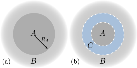
Figure 1: (Color online) Schematic description of (a) the partitioning of space for the phase space method and (b) the mask method. Region $A$ is the interaction region, $B$ is the Volkov propagation region and $C$ is the overlap region where $\Psi_{A}$ and $\Psi_{B}$ mix under the mask function.

The quantum phase-space naturally leads to a geometrical interpretation of photoemission. One could think to divide the space in two regions $A$ and $B$ as in Fig. 1 (a), where region $B$ represents the region where detectors are positioned and $A$ is defined as the complement of $B$. In this picture, PES can be seen as the probability to have an electron with given momentum in $B$. It is then natural to define the momentum-resolved photoelectron spectrum as

$$\mathcal{P}(\mathbf{p})=\lim_{t\rightarrow\infty}\int_{B}\mathtt{d}\mathbf{R}\,w({\bf R},{\bf p},t)$$ (4)

where the spatial integration is carried out in region $B$, and the limit $t\rightarrow\infty$ assures that region $B$ contains all photoelectron contributions. From the knowledge of the momentum-resolved PES [cf. Eq. (4)] one can access several different quantities by simple integration. For instance, in three dimensions ($d=3$) the energy-resolved PES is obtained integrating over the solid angle $\Omega$:

$$P(E=p^{2}/2)=\int_{0}^{4\pi}{\rm d}\Omega\,\mathcal{P}(\mathbf{p})\,,$$ (5)

and the photoelectron angular distribution in the system reference frame is given by,

$$P(E=p^{2}/2,\theta)=\int_{0}^{2\pi}{\rm d}\phi\,\mathcal{P}(\mathbf{p})\,.$$ (6)

In spite of giving an intuitive picture of PES, Eq. (4) is not suited for direct numerical evaluation since it requires the knowledge of the full one-body density matrix in the whole space. In the next section we will make a contact with effective single particle theories like TDDFT to overcome the limitations due to the knowledge of the many-body wavefunction. In order to avoid integration over the whole space an efficient evolution scheme is presented in Sect. II.3.

II.2 Phase space interpretation within TDDFT

TDDFT is an effective single particle theory where the many-body wavefunction is described by an auxiliary single Slater determinant $\Psi_{KS}(\mathbf{r_{1}},\dots,\mathbf{r_{N}})$ built out of Kohn-Sham orbitals $\psi_{i}(\mathbf{r})$ Runge and Gross (1984); Marques et al. (2011). In order to simplify the notation, we drop the explicit time dependence from the wavefunctions and assume that the following equations are written in the limit $t\rightarrow\infty$ as prescribed by Eq. (4).

Being represented by a single determinant, the one-body Kohn-Sham density matrix is given by

$$\rho_{KS}(\mathbf{r},\mathbf{r}^{\prime})=\sum_{i=1}^{\rm occ.}\psi_{i}(\mathbf{r})\psi_{i}(\mathbf{r}^{\prime})$$ (7)

where the sum in carried out over all occupied orbitals. Performing a decomposition of each orbital according to the partition of Fig. 1 (a) we obtain

$$\psi_{i}(\mathbf{r})=\psi_{A,i}(\mathbf{r})+\psi_{B,i}(\mathbf{r})\,,$$ (8)

where $\Psi_{A,i}(\mathbf{r})$ is the part of the wavefunction describing states localized in $A$ and $\Psi_{B,i}(\mathbf{r})$ is the ionized contribution measured at the detector in $B$. The one-body density matrix can now be accordingly decomposed as a sum of four terms

$$\rho_{KS}(\mathbf{r},\mathbf{r}^{\prime})=\sum_{i=1}^{\rm occ.}\left[\psi_{A,i}(\mathbf{r})\psi_{A,i}^{*}(\mathbf{r}^{\prime})+\psi_{A,i}(\mathbf{r})\psi_{B,i}^{*}(\mathbf{r}^{\prime})\right.\\ +\left.\psi_{B,i}(\mathbf{r})\psi_{A,i}^{*}(\mathbf{r}^{\prime})+\psi_{B,i}(\mathbf{r})\psi_{B,i}^{*}(\mathbf{r}^{\prime})\right].$$ (9)

From Eq. (9) we can build the KS Wigner function defined in Eq. (2) and obtain the momentum-resolved probability distribution by inserting it into Eq. (4). We note that this step involves a non-trivial approximation, namely that the KS one-body density matrix is a good approximation to the fully interacting one in region B. This is, however, much milder than the assumption that the Kohn-Sham determinant is a good approximation to the many-body wavefunction in region B, as it is done, e.g., in the SPM.

The final result is a sum of four overlap double integrals that can be simplified further. For a detailed calculation we refer to Appendix A. The first overlap integral, containing a product of two functions localized in $A$ [cf. Eq. (9)], is zero due to the spatial integration in $B$. The two next overlap integrals, containing mixed products of wavefunctions localized in $A$ and $B$, can be reduced by increasing the size of region $A$. Assuming $A$ to be large enough to render these terms negligible the only integral we are left with is the one containing functions in $B$, leading to

$$\mathcal{P}(\mathbf{p})\approx\int_{B}{\rm d}\mathbf{R}\,\int\frac{{\rm d}\mathbf{s}}{(2\pi)^{\frac{d}{2}}}\,e^{i\mathbf{p}\cdot\mathbf{s}}\\ \sum_{i=1}^{\rm occ.}\psi_{B,i}(\mathbf{R}+\frac{\mathbf{s}}{2})\psi_{B,i}^{*}(\mathbf{R}-\frac{\mathbf{s}}{2})\,.$$ (10)

The approximation sign $\approx$ is a reminder for the error committed in discarding the mixed overlap integrals. Since the probability of finding an ionized electron in region $A$ is zero for $t\rightarrow\infty$, we can extend the integration over $B$ in Eq. (10) to the whole space. Using the integral properties of the Wigner transform we finally obtain

$$\mathcal{P}(\mathbf{p})\approx\sum_{i=1}^{\rm occ.}\left|\tilde{\psi}_{B,i}(\mathbf{p})\right|^{2}\,,$$ (11)

where $\tilde{\psi}_{B,i}(\mathbf{p})$ is the Fourier transform of $\psi_{B,i}(\mathbf{r})$ and the expression is written in the limit for $t\rightarrow\infty$. Equation (11) gives an intuitive formulation of momentum-resolved PES as a sum of the Fourier component of each orbital in the detector region. It is worth to note that Eq. (11) is not restricted to TDDFT and can be applied to other effective single-particle formulations such as time-dependent Hartree-Fock and the TDSE in the SAE approximation.

The numerical evaluation of the ionization probability from Eq. (11) requires the knowledge of the wavefunction after the external field has been switched off. For ionization processes this means that one has to deal with simulation boxes that extend over several hundred atomic units and this practically constrains the method only to one-dimensional calculations. In the next section we will derive a simple scheme to overcome this limitation making the present scheme applicable for realistic simulations of molecules and nanostructures.

II.3 The mask method

In the previous sections we described a practical way to evaluate the momentum-resolved PES following the spatial partitioning of Fig. 1 (a) and how this can be conveniently cast in the language of TDDFT. In this section we take a step further in developing an efficient time evolution scheme by exploiting the geometry of the problem together with some physical assumptions.

We start by introducing a split-evolution scheme: At each time $t$ we implement a spatial partitioning of Eq. (8) as following

$$\left\{\begin{array}[]{ll}\psi_{A,i}(\textbf{r},t)=M(\textbf{r})\psi_{i}(\textbf{r},t)\\ \psi_{B,i}(\textbf{r},t)=[1-M(\textbf{r})]\psi_{i}(\textbf{r},t)\end{array}\right.\,,$$ (12)

where $M(\mathbf{r})$ is a smooth mask function defined to be 1 deep in the interior of region $A$ and 0 outside, as shown in Fig. 2.

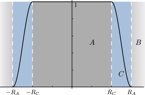
Figure 2: (Color online) The mask function implements a smooth transition from region $A$ to region $B$. The functional shape used for actual calculations is defined in Eq. (18).

Such a mask function, along with the partitions $A$ and $B$, introduces a buffer region $C$ (technically handled as the outermost shell of $A$), where $\psi_{A,i}(\textbf{r},t)$ and $\psi_{B,i}(\textbf{r},t)$ overlap [see Fig. 1 (b)].

We can set up a propagation scheme from time $t$ to $t^{\prime}$ as following

$$\left\{\begin{array}[]{ll}\psi_{A,i}(\textbf{r},t^{\prime})=M(\textbf{r})U(t^{\prime},t)\left[\psi_{A,i}(\textbf{r},t)+\psi_{B,i}(\textbf{r},t)\right]\\ \psi_{B,i}(\textbf{r},t^{\prime})=[1-M(\textbf{r})]U(t^{\prime},t)\left[\psi_{A,i}(\textbf{r},t)+\psi_{B,i}(\textbf{r},t)\right]\end{array}\right.$$ (13)

where $U(t^{\prime},t)$ is the time propagator associated with the full Hamiltonian including the external fields. Equation (13) defines a recursive propagation scheme completely equivalent to a time propagation in the whole space $A\cup B$.

In typical experimental setups, detectors are situated far away from the sample and electrons overcoming the ionization barrier travel a long way before being detected. During their journey toward the detector, and far away from the molecular system, they practically evolve as free particles driven by an external field. It seems therefore a waste of resources to solve the full Schrödinger equation for the traveling electrons while their behavior can be described analytically. In addition, an ideal detector placed relatively close to the molecular region would measure the same PES.

From these observations we conclude that we can reduce region $A$ to the size of the interaction region and assume electrons in $B$ to be well described by non-interacting Volkov states. Volkov states are the exact solution of the Schrödinger equation for free electrons in an oscillating field. They are plane-waves and are therefore naturally described in momentum space. In the velocity gauge the Volkov time propagator is formally expressed by

$$U_{V}(t^{\prime},t)=\exp\left\{-i\int_{t}^{t^{\prime}}{\rm d}\tau\,\frac{1}{2}\left[\mathbf{p}-\frac{\mathbf{A}(\tau)}{c}\right]^{2}\right\}\,,$$ (14)

where the time-ordering operator is omitted for brevity and $\mathbf{A}(\tau)$ is the vector potential. This is equivalent to the use of a strong-field approximation in the outer region in the same spirit of the Lewenstein model Lewenstein et al. (1994).

In summary, the method we propose consists in solving numerically the real-space TDDFT equations in $A$ and analytically propagating the wavefunctions residing in $B$ in momentum space. In this setup region $C$ acts as a communication layer between functions in $A$ and $B$. Under this prescription, and by handling $B$-functions in momentum space, Eq. (13) becomes

$$\left\{\begin{array}[]{ll}\psi_{A,i}(\textbf{r},t^{\prime})=\eta_{A,i}(\textbf{r},t^{\prime})+\eta_{B,i}(\textbf{r},t^{\prime})\\ \tilde{\psi}_{B,i}(\textbf{p},t^{\prime})=\tilde{\xi}_{A,i}(\textbf{p},t^{\prime})+\tilde{\xi}_{B,i}(\textbf{p},t^{\prime})\end{array}\right.$$ (15)

with

$$\eta_{A,i}(\textbf{r},t^{\prime})= M(\textbf{r})U(t^{\prime},t)\psi_{A,i}(\textbf{r},t)$$ (16a)

$$\eta_{B,i}(\textbf{r},t^{\prime})= M(\textbf{r})\int\frac{{\rm d}\mathbf{p}\,e^{i\mathbf{p}\cdot\mathbf{r}}}{(2\pi)^{\frac{d}{2}}}U_{V}(t^{\prime},t)\tilde{\psi}_{B,i}(\textbf{p},t)$$ (16b)

$$\tilde{\xi}_{A,i}(\textbf{p},t^{\prime})= \int\frac{{\rm d}\mathbf{r}\,e^{-i\mathbf{p}\cdot\mathbf{r}}}{(2\pi)^{\frac{d}{2}}}$$

$$\times[1-M(\textbf{r})]U(t^{\prime},t)\psi_{A,i}(\textbf{r},t)$$ (16c)

$$\tilde{\xi}_{B,i}(\textbf{p},t^{\prime})= U_{V}(t^{\prime},t)\tilde{\psi}_{B,i}(\textbf{p},t)$$

$$-\int\frac{{\rm d}\mathbf{r}\,e^{-i\mathbf{p}\cdot\mathbf{r}}}{(2\pi)^{\frac{d}{2}}}\eta_{B,i}(\textbf{r},t^{\prime})\,.$$ (16d)

At each time step the orbital $\psi_{A,i}$ is evolved under the mask function and stored in $\eta_{A,i}$, forcing $\eta_{A,i}$ to be localized in $A$. At the same time, the components of $\psi_{A,i}$ escaping from $A$ are collected in momentum space by $\tilde{\xi}_{A,i}$. We then add to $\tilde{\xi}_{A,i}$ the contribution of the wavefunctions already present in $B$ at time $t$ by summing up $U_{V}\tilde{\psi}_{B,i}$. In order to allow electrons to come back from $B$ to $A$ we include $\eta_{B,i}$ in $A$ and correct the function in $B$ by removing its Fourier components [second term in Eq. (16d)].

One of the advantages of Eq. (15) is that all the spatial integrals present in $\eta_{B,i}(\textbf{r},t^{\prime})$ and $\tilde{\xi}_{B,i}(\textbf{p},t^{\prime})$ are performed on functions localized in $C$. Therefore, integrals over the whole space are evaluated at the cost of an integration on the much smaller buffer region $C$ that can be easily evaluated by fast Fourier transform algorithms. Similar considerations hold for integrals in momentum space under the assumption that $B$-functions $\tilde{\psi}_{B,i}(\mathbf{p},t)$ are localized in momentum. When region $A$ is discretized on a grid, in order to avoid wavefunction wrapping at the boundaries and preserve numerical stability, additional care must be taken. In our implementation, numerical stability is addressed by the use of non-uniform Fourier transforms (see details in Appendix B).

There are situations were the electron flow from $B$ to $A$ is negligible. This is the case, for instance, when $A$ is large enough to contain the whole wavefunctions at the time when the external field has been switched off. A propagation at later times will see photoelectrons flowing mainly from $A$ to $B$. In this situation, $\eta_{B,i}$ and the corresponding correction term in $\tilde{\xi}_{B,i}$ can be discarded. The evolution scheme of Eq. (15) is thus simplified and becomes

$$\left\{\begin{array}[]{ll}\psi_{A,i}(\textbf{r},t^{\prime})=\eta_{A,i}(\textbf{r},t^{\prime})\\ \tilde{\psi}_{B,i}(\textbf{p},t^{\prime})=\tilde{\xi}_{A,i}(\textbf{p},t^{\prime})+U_{V}(t^{\prime},t)\tilde{\psi}_{B,i}(\textbf{p},t)\end{array}\right.$$ (17)

In the folowing we will refer to Eq. (17) as the “mask method” (MM), and to Eq. (15) as the “full mask method” (FMM). We note here again that, being single-particle propagations schemes, both MM and FMM are not restricted to TDDFT and can be applied to other effective single-particle theories. As a matter of fact an approach similar to Eq. (17) has already been employed in the propagation of the TDSE equations for atomic systems Chelkowski et al. (1998); Grobe et al. (1999); Tong et al. (2006), and in TDDFT for one-dimensional models of metal surfaces Varsano et al. (2004). We also note that the implementation of absorbing boundaries trough a mask function as done in Eq. (16a) can be cast in terms of an additional imaginary potential (exterior complex scaling) in the Schrödinger equation. Such approach is commonly used in quantum optics.

Within the MM, the evolution in $A$ is completely unaffected by the wavefunctions in $B$ and ionized electrons are treated uniquely in momentum space. Compared with the FMM, the MM is numerically more stable as it is not affected by boundary wrapping. In order to achieve the conditions where Eq. (17) is valid may require, however, large simulation boxes. Moreover as the mask function never absorbs perfectly the electrons, spurious reflections may appear. Suppression of such artifacts requires a further enlargement of the buffer region. With FMM spurious reflections are almost negligible.

Choosing between MM and FMM implies a tradeoff between computational complexity and numerical stability that strongly depends on the ionization dynamics of the process under study. In what follows, we will illustrate the differences and devise a prescription to help the choice of the most suitable method in each specific case.

III Applications

In this section we present a few numerical applications of the schemes previously derived. In all calculations the boundary between $A$ and $B$ regions is chosen as a $d$-dimensional sphere implemented by the mask function:

$$M(\mathbf{r})=\left\{\begin{array}[]{ll}1&\mbox{if $r<R_{C}$}\\ 1-\sin^{2}\left(\frac{(r-R_{C})\pi}{2(R_{A}-R_{C})}\right)&\mbox{if $R_{C}\leq r\leq R_{A}$}\\ 0&\mbox{if $r>R_{A}$}\end{array}\right.\,,$$ (18)

as shown in Fig. 2. Note that numerical studies (not presented here) revealed a weak dependence of the final results on the functional shape of the mask.

The time propagation of the orbitals in $A$ is performed with the enforced time-reversal symmetry evolution operator Castro et al. (2004)

$$U(t+\Delta t,t)=\exp\left(-i\frac{\Delta t}{2}H(t+\Delta t)\right)\exp\left(-i\frac{\Delta t}{2}H(t)\right)\,,$$ (19)

where $H$ is the full KS Hamiltonian, and the coupling with the external field is expressed in the velocity gauge.

The first system we will study is hydrogen. In spite of being a one-electron system, it is a seemingly trivial case that has been and still is under thorough theoretical investigation Burenkov et al. (2010); Grum-Grzhimailo et al. (2010); Ivanov (2011); Zhou and Chu (2011); Pullen et al. (2011); Zheng et al. (2012); Tao and Scrinzi (2012). Clearly we do not need TDDFT to study hydrogen and our numerical results are obtained by propagating the wavefunction with a non-interacting Hamiltonian. The interest in this case is focused on the numerical performance of different mask methods as hydrogen provides a useful benchmark.

The full TDDFT calculations performed for molecular nitrogen, carbon monoxide, and benzene are later presented in Sect. III.2 and Sect. III.3 respectively. In these cases, norm-conserving Troullier-Martins pseudopotentials and the exchange-correlation LB94 potential van Leeuwen and Baerends (1994) (that has the correct asymptotic limit for molecular systems) are employed. Finally, in all calculations the starting electronic structure of the molecules is calculated in the Born-Oppenheimer approximation at the experimental equilibrium geometry and the time evolution is performed with fixed ions.

III.1 Photoelectron spectrum of hydrogen

As first example we study multi-photon ionization of a one-dimensional soft-core hydrogen atom, initially in the ground state, and exposed to a $\lambda=532$ nm ($\omega=0.0856$ a.u.) linearly polarized laser pulse with peak intensity $I=1.38\times 10^{13}$ ${\rm W}/{\rm cm}^{2}$, of the form

$$A(t)=A_{0}f(t)\cos(\omega t)$$ (20)

where $f(t)$ is a trapezoidal envelope function of 14 optical cycles with two-cycle linear ramps, constant for 10 cycles, and with $A_{0}=31.7$ a.u. Here $A(t)$ is the vector potential in units of the speed of light $c$. A soft-Coulomb potential $V(x)=-1/\sqrt{2+x^{2}}$ is employed to model the electron-ion interaction. We propagate the electronic wavefunction in time and then compare the energy-resolved ionization probability obtained from different schemes. Along with MM, FMM, and SPM we present results for direct evaluation of PES from Eq. (5). In this method the spectrum is obtained by directly Fourier transforming the wavefunction in region B. Since the analysis is conducted without perturbing the evolution of the wavefunction we will refer to it as the “passive method” (PM). This method requires the knowledge of the whole wavefunction after the pulse has been switched off, and since a considerable part of the wave-packet is far away from the core (for the present case a box of 500 a.u. radius is needed for 18 optical cycles), it is viable only for one-dimensional calculations. Nevertheless it is important as it constitutes the limiting case for both MM and FMM.

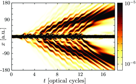
Figure 3: (Color online) Evolution of the electronic density as a function of time $\rho(x,t)=|\psi(x,t)|^{2}$ for the one-dimensional soft-core hydrogen model. The laser pulse has angular frequency $\omega=0.0856$ a.u., intensity $I=1.38\times 10^{13}$ ${\rm W}/{\rm cm}^{2}$, and a trapezoidal envelope with 2 optical cycle linear ramp (one optical cycle $=1.774$ fs) and 10 cycles constant center.

In Fig. 3, a color plot of the evolution of the electronic density as a function of time is shown. The electronic wavefunction splits into sub-packets generated at each laser cycle (one optical cycle $=2\pi/\omega=1.774$ fs). These wavepackets evolve in bundles and their slope correspond to a certain average momentum. ATI peaks are then formed by the build up of interfering wavepackets periodically emitted in the laser field and leading to a given final momentum Schwengelbeck and Faisal (1994).

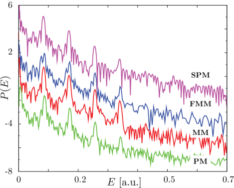
Figure 4: (Color online) Energy resolved photoelectron probability $P(E)$ (logarithmic scale) calculated with different approaches. The spectra are shifted by multiplying a constant factor for easy comparison. From bottom to top: passive method Eq. (5) in green, mask method Eq. (17) in red, full mask method Eq. (15) in blue, and sampling point method Eq. (1) in purple. Laser parameters are the same as in Fig. 3.

From Fig. 3 is it possible to see that electrons may be considered as escaped “already” at 30 a.u. away from the center. We set therefore $R_{A}=30$ a.u. and calculate energy-resolved PES with the PM. As we can see from Fig. 4 the spectrum presents several peaks at integer multiples of $\omega$ following $E=s\omega-I_{P}-U_{P}$ with $U_{P}=A_{0}^{2}/4c^{2}=0.0133$ a.u. being the ponderomotive energy, $I_{P}=0.5$ a.u. the ionization potential, and $s$ the number of absorbed photons. In this case the minimum number of photons needed to exceed the ionization threshold is $s=6$. Of course, the spectrum is only in qualitative agreement with three-dimensional calculations Schafer and Kulander (1990) as expected from a one-dimensional soft-core model Kästner et al. (2010); Gordon et al. (2005); Schwengelbeck and Faisal (1994).

PES calculated from MM, FMM, and SPM all agree as reported in Fig. 4. Numerical calculations were performed until convergence was achieved, leading to a grid with spacing $\Delta R=0.4$ a.u. and box sizes depending on the method. For MM we employed a simulation box of $R_{A}=70$ a.u. and set the buffer region at $R_{C}=30$ a.u. In order to have energy resolution comparable with PM we used padding factors (see Appendix B) $P=P_{N}=4$ and the total simulation time was $T=18$ optical cycles. For FMM a smaller box of $R_{A}=40$ a.u. with $R_{C}=30$ a.u. is needed to converge results, and $P=8$, $P_{N}=2$ were needed to preserve numerical stability for $T=18$ optical cycles. For SPM two sampling points at $r_{S}=-500,500$ a.u. were needed to get converged results with a box of 550 a.u., and a complex absorberKosloff and Kosloff (1986); Jhala et al. (2010) at 49 a.u. from the boundaries of the box. In addition, a total time of $T=74$ optical cycles was required to collect all the wave packets. The need for such a huge box resides on the working conditions of SPM. In order to avoid spurious effects, the sampling points must be set at a distance such that the density front arrives after the external field has been switched off. Therefore the longer the pulse the further away the sampling points must be set. For these laser parameters one could rank each method according to increasing numerical cost starting from MM, followed by FMM, PM, and SPM.

As a second example we study the ionization of this one dimensional hydrogen atom by an ultra-short intense infrared laser. We employ a single two-cycle pulse of wavelength $\lambda=800$ nm ($\omega=0.057$ a.u.), intensity $I=2.5\times 10^{14}$ ${\rm W}/{\rm cm}^{2}$, and envelope

$$f(t)=\left\{\begin{array}[]{ll}-\sin(\omega t/2N_{c})^{2}&\mbox{if $0\leq t\leq 2\pi N_{c}/\omega$}\\ 0&\mbox{if $t>2\pi N_{c}/\omega$}\end{array}\right.$$ (21)

with $N_{c}=2$ and $A_{0}=225.8$ a.u.

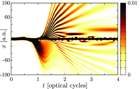
Figure 5: (Color online) Density evolution $\rho(x,t)$ for a one-dimensional soft-core hydrogen and a two-cycle $\sin^{2}$ laser pulse with angular frequency $\omega=0.057$ a.u., and intensity $I=2.5\times 10^{14}$ ${\rm W}/{\rm cm}^{2}$. Here one optical cycle $=2.66$ fs.

Due to the laser strength and long wavelength, the electron evolution shown Fig. 5 is quite different from the one presented before. Electrons ejected from the core are driven by the laser and follow wide trajectories before returning to the parent ion. Such trajectories can be understood in the context of the semiclassical model Corkum (1993) where released electrons move as a free particle in a time-dependent field with a maximum oscillation amplitude of $x_{0}=2A_{0}/\omega c=57.8$ a.u. Electrons ejected near a maximum of the electric field $\epsilon(t)=-\partial A(t)/\partial t$ are the ones gaining the most kinetic energy and are therefore responsible for the fast emerging electrons after rescattering with the core.

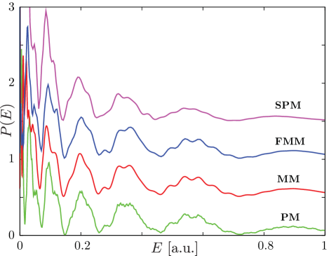
Figure 6: (Color online) Energy-resolved photoelectron $P(E)$ yield from different approaches. Spectra are shifted by a constant factor. Order and color coding is the same as in Fig. 4. Laser parameters are described in the caption of Fig. 5.

In Fig. 6 we show the energy-resolved PES for different methods. Here the spectra appear to be very far from any ATI structure due to short duration of the laser pulse and is characterized by some irregular maxima and minima Burenkov et al. (2010). The characteristic features of the ionization dynamics is strongly dependent on the detailed shape of the pulse as one can easily imagine by inspecting the asymmetry in the electron ejection from Fig. 5. Due to these dynamics, a dramatic carrier envelope phase dependence for such short pulses is expected.

All the different methods result in similar spectra but with different parameters. In PM we set $R_{A}=50$ a.u. and a box of radius $R=700$ a.u. is needed to contain the wave function after $T=4$ optical cycles (one optical cycle $=2.66$ fs). For MM $R_{A}=200$ a.u., $R_{C}=40$ a.u., and the padding factors are $P=2$, $P_{N}=4$. Here the value for $R_{A}$ is dictated by the width of the buffer region which needs to be wide enough to prevent spurious reflections.

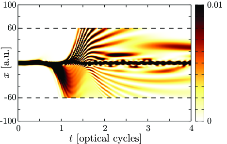
Figure 7: (Color online) FMM density evolution $|\psi_{A}(x,t)|^{2}$ of a one-dimensional soft-core hydrogen. Laser parameters are the same as in Fig. 5. Dashed lines indicate the edges of the simulation box.

A considerably smaller box is needed for FMM, where $R_{A}=60$ a.u., $R_{C}=40$ a.u., $P=4$, and $P_{N}=2$. In this case one can reconstruct the total density in $A$ by evaluating $|\psi_{A}(x,t)|^{2}$ via Eq. (15) and compare it to the exact evolution. As one can see in Fig. 7 the reconstructed density displays a behavior remarkably similar to the exact one of Fig. 5 but with a considerably reduced computational cost. SMP requires sampling points at $r_{S}=-130,130$ a.u. in a box of radius $R=200$ a.u. with 49 a.u. wide complex adsorbers, and for a total time of $T=7$ optical cycles.

The possibility to use relatively small simulation boxes is especially important for three-dimensional calculations where the computational cost scales with the third power of the box size. Both mask methods are practicable options for 3D simulations and the advantage of using FMM with respect to MM is driven by the electron dynamics. For long laser pulses MM appears to be more stable and it is a better choice than FMM, while for short pulses with large electron oscillations FMM can be more performant. SPM is a viable option for short pulses and small values for the oscillations.

As a last example, we present ATI of a real three-dimensional hydrogen atom subject to a long infrared pulse. We employ a laser linearly polarized along the $x$-axis with wavelength $\lambda=800$ nm, intensity $I=5\times 10^{13}$ ${\rm W}/{\rm cm}^{2}$, pulse shape of the form (21) with $N_{c}=20$ and $A_{0}=91.3$ a.u. Due to to the pulse length, MM appears to be the most appropriate choice in this case. In the calculation $R_{A}=60$ a.u., $R_{C}=50$ a.u., $P=1$ and $P_{N}=8$.

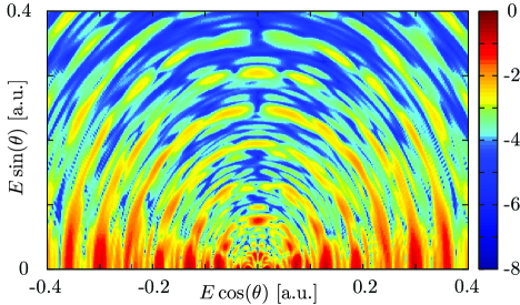
Figure 8: (Color online) Photoelectron angular distribution $P(E,\theta)$ (logarithmic scale) of hydrogen for a 20 cycle $\sin^{2}$ laser pulse of wavelength $\lambda=800$ nm, and intensity $I=5\times 10^{13}$ ${\rm W}/{\rm cm}^{2}$ polarized along the $x$ axis.

In Fig. 8 we show a high-resolution density plot of the PAD $P(E,\theta)$ defined in Eq. (6). The radial distance denotes the photoelectron energy while the angle indicates the direction of emission with respect to the laser polarization. The color density is plotted in logarithmic scale and represents the values of $P(E,\theta)$.

The photoelectron energy-angular distribution displays complex interference patterns. The pattern shape compares favorably with similar calculations in the literature Arbó et al. (2008); Telnov and Chu (2009b); Zhou and Chu (2011); Tao and Scrinzi (2012). It consists of a series of rings with fine structures. Each ring represents the angular distribution of the photoelectron ATI peaks. The spacing of adjacent rings equals the photon energy $\omega=0.057$ a.u. Photoelectrons are emitted mainly along the laser polarization, and the left-right symmetry of the rings indicates that the photoelectrons do not present any preferential ejection side with respect to the polarization axis. The first ring corresponds to the angular distribution of the first ATI peak. It presents a peculiar nodal pattern that is induced by the long-range Coulomb potential and is related to the fact that the ATI peak is determined by one dominant partial wave in the final state Arbó et al. (2006). The number of the stripes equals the angular momentum quantum number of the dominant partial wave in the final state plus one Arbó et al. (2006). In Fig. 8, the first ring contains six stripes and the dominant final state has angular momentum quantum number of 5. The pattern of the energy-angular distribution and the stripe number of the first ring are in good agreement with those in the literature Telnov and Chu (2009b); Zhou and Chu (2011). As for the fine structures, we observe that while the main ring pattern is already formed in the first half of the pulse, the fine structure builds up until the end of the pulse. This supports the hypothesis that such structures are induced by the coherence of the two contributions from the leading and trailing edges of the pulse envelope Telnov and Chu (2009b).

III.2 N₂ under a few-cycle infrared laser pulse

In this section we compare theoretical and experimental angular resolved photoelectron probabilities for randomly oriented N₂ molecules. We choose the laser parameters according to experiment Gazibegović-Busuladžić et al. (2011), i.e., we employ a $N_{c}=6$ cycle pulse of wavelength $\lambda=750$ nm ($\omega=0.06$ a.u.), intensity $I=4.3\times 10^{13}$ ${\rm W/cm}^{2}$. A laser shape

$${\bf A}(t)=\left\{\begin{array}[]{ll}\frac{{\bf A}_{0}}{2}(1-\cos(\frac{\omega t}{N_{c}}))\sin(\omega t)&\mbox{if $0\leq t\leq 2\pi N_{c}/\omega$}\\ 0&\mbox{if $t>2\pi N_{c}/\omega$}\end{array}\right.$$ (22)

for the vector potential should lead to an electric field similar to the one employed in the experiment with zero carrier envelope phase.

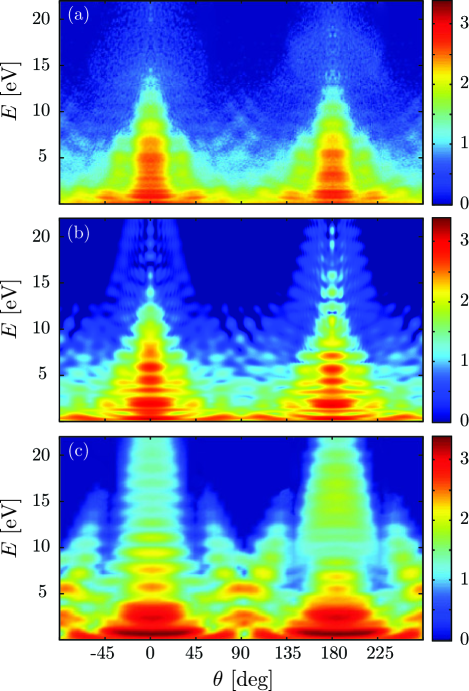
Figure 9: (Color online) Photoelectron angle and energy resolved probability $\bar{P}(E,\theta)$ (log scale) in the laboratory frame for randomly oriented N₂ molecules in a 6 cycles infrared laser pulse with $\lambda=750$ nm, with intensity $I=4.3\times 10^{13}$ ${\rm W/cm}^{2}$. The angle $\theta$ is measured from the laser polarization axis. The different panels represent $\bar{P}(E,\theta)$ (spanning 3.4 orders of magnitude), from (a) experiment, (b) calculated with TDDFT and FMM, and (c) calculated with modified molecular strong field approximation. Panels (a) and (c) are adapted from Ref. Gazibegović-Busuladžić et al., 2011.

In Fig. 9 (a) the experimental photoelectron probability $\bar{P}(E,\theta)$ is plotted in logarithmic scale as a function of the energy and the angle with respect to the laser polarization in the laboratory frame. Electrons are mainly emitted at small angles, and, due to the short nature of the pulse electron emission is asymmetric along the laser polarization axis (at angles close to $0^{\circ}$ and $180^{\circ}$).

We performed TDDFT calculations for different angles $\theta_{L}$ between the molecular axis and the laser polarization. The molecular geometry was set at the experimental equilibrium interatomic distance $R_{0}=2.074$ a.u. The Kohn-Sham wavefunctions were expanded in real space with spacing $\Delta r=0.38$ a.u. in a simulation box of $R_{A}=35$ a.u. The photoelectron spectra were calculated with FMM having $R_{C}=25$ a.u., and padding factors $P=1$, and $P_{N}=4$.

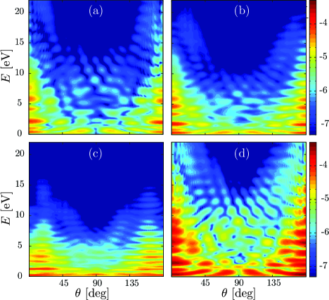
Figure 10: (Color online) Photoelectron angle and energy resolved probability $P_{\theta_{L}}(E,\theta)$ (log scale) for aligned N₂ molecules and different laser polarization directions $\theta_{L}$: (a) $\theta_{L}=90^{\circ}$, (b) $\theta_{L}=60^{\circ}$, (c) $\theta_{L}=30^{\circ}$, (d) $\theta_{L}=0^{\circ}$. Here $\theta_{L}$ is the angle between the laser polarization direction and the molecular axis. Laser parameters are the same as in Fig. 9.

In Fig. 10 the logarithmic ionization probability $P_{\theta_{L}}(E,\theta)$ is plotted as a function of energy $E$ and angle $\theta$ measured from the laser polarization axis for different values of $\theta_{L}$. As the molecular orientation decreases from $90^{\circ}\leq\theta_{L}\leq 30^{\circ}$ we observe an increasing suppression of the emission together with a shift of the maximum that moves away from the laser polarization axis. For $\theta_{L}=0^{\circ}$ the emission is highly enhanced for all angles and peaked along the laser direction. The signature of multi-center emission interference has been predicted to be particularly marked when the laser polarization is perpendicular to the molecular axis Busuladžić et al. (2008a, b) (i.e. $\theta_{L}=90^{\circ}$). However, the lowest point in energy of such a pattern is predicted for $\theta=90^{\circ}$ and $E=\pi^{2}/2R_{0}^{2}\approx 31$ eV, way above the energy window of observable photoelectrons produced by our laser. A stronger and longer laser pulse would be required to extend the rescattering plateau toward higher energies and therefore to reveal the pattern Okunishi et al. (2009).

In order to reproduce the experimental $\bar{P}(E,\theta)$, an average over all the possible molecular orientations should be performed. Due to the axial symmetry of the molecule we can restrict the average to $0\leq\theta_{L}\leq 90^{\circ}$ and integrate all the contributions with the proper probability weight Wopperer et al. (2010b)

$$\bar{P}(E,\theta)\propto\int_{0}^{90^{\circ}}{\rm d}\theta_{L}\,\sin\theta_{L}\,P_{\theta_{L}}(E,\theta)\,.$$ (23)

We evaluate Eq. (23) by discretizing the integral in a sum for $\theta_{L}=0^{\circ},30^{\circ},60^{\circ},90^{\circ}$, and display the result in Fig. 9 (b). Even in this crude approximation, and without taking into account focal averaging, the agreement with the experiment is satisfactory and compares favorably to the molecular strong field approximation shown in Fig. 9 (c). The agreement deteriorates for low energies where the importance of the Coulomb tail is enhanced as it is not fully accounted due to limited dimensions of the simulation box. As a matter of fact the agreement greatly increases for higher energies.

III.3 He-(I) PADs for carbon monoxide and benzene

In this section we deal with UV ($\omega=0.78$ a.u.) angular resolved photoemission triggered by weak lasers. When the external field is weak, non-linear effects can be discarded and first order perturbation theory can be applied. In this situation, the momentum resolved PES can be evaluated by Fermi’s golden rule as

$$P(\mathbf{p})\propto\sum_{i}|\langle\Psi_{f}|\mathbf{A}_{0}\cdot\mathbf{p}|\Psi_{i}\rangle|^{2}\delta(E_{f}-E_{i}-\omega)\,,$$ (24)

where $|\Psi_{i}\rangle$ ($|\Psi_{f}\rangle$) is the initial (final) many-body wavefunction of the system and $\mathbf{A}_{0}$ is the laser polarization axis. The difficulty in evaluating Eq. (24) lies in the proper treatment of the final state, which in principle belongs to the continuum of the same Hamiltonian of $|\Psi_{i}\rangle$. In the simplest approach, it is approximated by a plane wave (PW). In this approximation the square root of the momentum-resolved PES is proportional to the sum of the Fourier transforms of the initial state wavefunctions $\tilde{\Psi}_{i}(\mathbf{p})$ corrected by a geometrical factor $|\mathbf{A}_{0}\cdot\mathbf{p}|$

$$\sqrt{P(\mathbf{p})}\propto\sum_{i}|\mathbf{A}_{0}\cdot\mathbf{p}|\times|\tilde{\Psi}_{i}(\mathbf{p})|\,.$$ (25)

If photoemission peaks are well resolved in momentum, individual initial states can be selectively measured. In this case a correspondence between momentum-resolved PES and electronic states in reciprocal space can be established. The range of applicability of the PW approximation has been discussed in the literature Puschnig et al. (2009). It has been postulated that Eq. (25) should be valid for (i) $\pi$-conjugated planar molecules, (ii) constituted by light atoms (H, C, N, O) and for (iii) photoelectrons emerging with momentum $\mathbf{p}$ almost parallel to the polarization axis.

Here we restrict ourselves to photoemission from the highest occupied molecular orbital (HOMO). In this case Eq. (25) becomes

$$\sqrt{P_{H}(\mathbf{p})}\propto|\mathbf{A}_{0}\cdot\mathbf{p}|\times|\tilde{\Psi}_{H}(\mathbf{p})|\,,$$ (26)

the subscript $H$ indicating HOMO-related quantities. We compare ab-initio TDDFT and PW PADs evaluated at fixed momentum $|\mathbf{p}_{H}|=\sqrt{2E_{H}}$ with $E_{H}=\omega-E_{B}$ being the kinetic energy of photoelectrons emitted from the HOMO and $E_{B}$ its binding energy.

TDDFT numerical calculations are carried out on a grid with spacing $\Delta r=0.28$ a.u. for benzene and $\Delta r=0.38$ a.u. for CO, in a simulation box of $R_{A}=30$ a.u.. Photoelectron spectra are calculated using MM with $R_{C}=20$ a.u. and padding factors $P=1$, $P_{N}=8$. A 40 cycles pulse with 8 cycle ramp at the He-(I) frequency $\omega=0.78$ a.u. and intensity $I=1\times 10^{8}$ ${\rm W/cm}^{2}$ is employed.

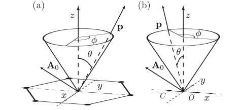
Figure 11: Photoemission geometries for oriented (a) benzene and (b) CO molecules.

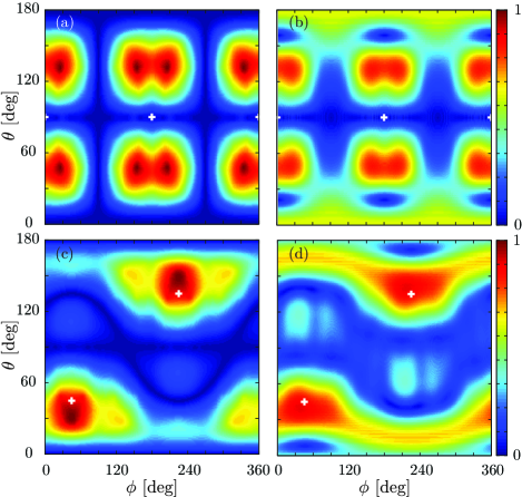
Figure 12: (Color online) He-(I) PADs for aligned benzene molecules. We compare PADs from PW $|\mathbf{A}_{0}\cdot\mathbf{p}||\tilde{\Psi}_{H}(\mathbf{p})|$ (left column) and TDDFT $\sqrt{P_{H}(\mathbf{p})}$ (right column) on a sphere at constant kinetic energy $E_{H}=0.363$ a.u. for different laser polarizations $\mathbf{A}_{0}$ (see text for details). Values on the sphere are normalized to unity. We used a 40 cycles (8 cycles ramp) UV trapezoidal laser pulse with $\lambda=58$ nm ($\omega=0.78$ a.u.), and intensity $I=1\times 10^{8}$ ${\rm W/cm}^{2}$. In the top row $\mathbf{A}_{0}=\hat{\mathbf{a}}_{1}=(1,0,0)$, and in the bottom row $\mathbf{A}_{0}=\hat{\mathbf{a}}_{2}=1/\sqrt{3}\times(1,1,1)$. White tics indicate the intersection of the laser polarization axis with the sphere at constant kinetic energy $E_{H}$. The geometry of the photoemission process is indicated in Fig. 11 (a).

We begin presenting the case of benzene since it constitutes the smallest molecule meeting all the conditions for Eq. (26) to be valid. Results for molecules oriented according to Fig. 11 (a), evaluated at $E_{H}=0.363$ a.u., and two different laser polarizations $\mathbf{A}_{0}=\hat{\mathbf{a}}_{1}$, $\hat{\mathbf{a}}_{2}$ with $\hat{\mathbf{a}}_{1}=(1,0,0)$, $\hat{\mathbf{a}}_{2}=1/\sqrt{3}\times(1,1,1)$, are shown in Fig. 12. In the case where the laser is polarized along the $x$ axis [see Fig. 12 (b)], PAD presents a four lobes symmetry separated by three horizontal and two vertical nodal lines. This structure is reminiscent of the HOMO $\pi$-symmetry with the nodal line at $\theta=90^{\circ}$ corresponding to the nodes of the orbital on the $x$-$y$ plane. Information on the orientation of the molecular plane could then be inferred from the inspection of this nodal line in the PAD. A similar feature can be observed also in the case of an off-plane polarization as shown in Fig. 12 (d). In this case, however, the laser can also excite $\sigma$-orbitals and the nodal line at $\theta=90^{\circ}$ is partially washed out. The other nodal lines can be understood in term of zeros of the polarization factor $|\mathbf{A}_{0}\cdot\mathbf{p}|$ and are thus purely geometrical. A PW approximation of the photoelectron distribution given by Eq. (26) qualitatively reproduce the ab-initio results as shown in Fig. 12 (a) and (d). According to condition (iii) a quantitative agreement is reached only for directions parallel to the polarization axis.

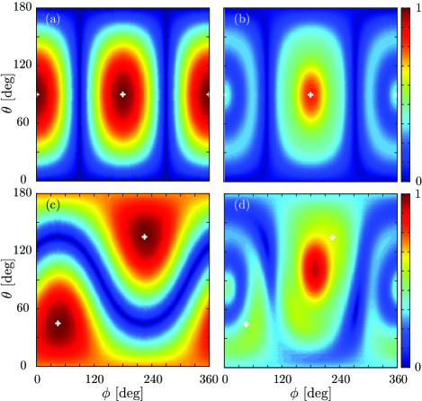
Figure 13: (Color online) He-(I) PADs for aligned CO molecules. Panel ordering and laser parameters are the same as in Fig. 12. The molecule is oriented according to Fig. 11 (b) and the photoelectron spectra were evaluated on a sphere at $E_{h}=0.261$ a.u.

A different behavior is expected in the case of CO. Photoelectrons with kinetic energy of $E_{H}=0.261$ a.u. are show in Fig. 13. In this case, condition (i) (i.e. $\pi$-conjugated molecule) is not fulfilled and a worse agreement between ab-initio and PW calculations is expected. The quality of the agreement can be assessed by comparing the left and right columns of Fig. 13. Here, the weak angular variation of $|\tilde{\Psi}_{H}(\mathbf{p})|$ is completely masked by the polarization factor $|\mathbf{A}_{0}\cdot\mathbf{p}|$ [cf. Fig. 13 (a) and (c)]. For this reason no information on the molecular configuration can be recovered from a PW model.

The situation is qualitatively different for TDDFT as, in this case, single atom electron emitters are fully accounted for. Here the nodal pattern is mainly governed by the polarization factor, but, however, fingerprints of the molecule electronic configuration can be detected. For instance, when the laser is polarized along the molecular axis, an asymmetry of the photoemission maxima can be observed for directions parallel to $\hat{\mathbf{a}}_{1}$ [see Fig. 13 (b)]. Here the global maximum is peaked around $(\phi,\theta)=(180^{\circ},90^{\circ})$ corresponding to the side of the carbon atom on the molecular axis [cf. Fig. 11 (b)]. These features can be again understood in terms of the shape of the HOMO. For CO, in fact, the HOMO is a $\sigma$ orbital with the electronic charge unevenly accumulated around the carbon atom. It is therefore natural to expect photoelectrons to be ejected mainly around the molecular axis and with higher probability form the side of the carbon atom. This asymmetry is therefore a property of the electronic configuration of the molecule and gives information about the molecular orientation itself. This behavior appears to be stable upon molecule rotation as can be observed in the case where the polarization is tilted with respect to the molecular axis [$\mathbf{A}_{0}=\hat{\mathbf{a}}_{1}$, see Fig. 13 (d)]. Even here the nodal structure is mainly dictated by the polarization factor.

IV Conclusions

In this work we studied the problem of photoemission in finite systems with TDDFT. We presented a formal derivation of a photoelectron density functional from a phase-space approach to photoemission. Such a functional can be directly applied to other theories based on a single Slater determinant and the derivation could serve as a base for extensions to more refined models.

We proposed a mixed real- and momentum-space evolution scheme based on geometrical splitting. In its complete form it allows particles to seamlessly pass back and forth from a real-space description to a momentum-space description. The ordinary splitting scheme turns out to be a special case of this more general method. Furthermore, we illustrated applications of the method on four physical systems: hydrogen, molecular nitrogen, carbon monoxide and benzene.

For hydrogen we presented a comparison of the different methods. We studied ATI peak formation in a one-dimensional model and ATI angular distributions for a three-dimensional case. The results turned out to be in good agreement with the literature. From the comparison, we derived a prescription to choose the best method based on a classification of the electron dynamics induced by the external field.

We investigated angular-resolved photoemission for randomly oriented N₂ molecules in a short intense IR laser pulse. We illustrated the results for four different molecular orientations with respect to the laser polarization. Owing to the symmetry of the problem we were able to combine the results to account for the random orientation. The spectrum for randomly oriented molecules is in good agreement with experimental measurements and is much better than the widely used strong field approximations (with one active electron) Gazibegović-Busuladžić et al. (2011).

We also studied UV angular resolved photoelectron spectra for oriented carbon monoxide and benzene molecules. We presented numerical calculations for two different directions of the laser polarization and compared with the plane-wave approximation. We found that the plane-wave approximation provides a good description for benzene while failing for CO. Furthermore, we found evidence that the photoelectron angular distribution carries important information on molecular orientation.

The successful implementation of photoelectron density functional presented in this Article paves the road for interesting applications to many different systems for a wide range of laser parameters. To name a few, TDDFT PAD could provide a theoretical tool superior to the plane-wave and the independent atomic center approximations to retrieve molecular adsorption orientation information from experiments. Atto-second pump probe experiments could be simulated ab-initio accounting for many-body effects but with great computational advantage with respect to full many-body methods and better physical description than SAE pictures.

V Acknowledgments

Special thanks to Lorenzo Stella for many stimulating discussions and suggestions. We also wish to acknowledge useful discussions and comments from Stefan Kurth, Ilya Tokatly, Matteo Gatti and Franck Lépine.

Financial support was provided by Spanish (FIS2011-65702-C02-01 and PIB2010US-00652 ), ACI-Promociona (ACI2009-1036), Grupos Consolidados UPV/EHU del Gobierno Vasco (IT-319-07), and the European Research Council Advanced Grant DYNamo (ERC-2010-AdG -Proposal No. 267374). Computational time was granted by i2basque and BSC “Red Espanola de Supercomputacion”. MALM acknowledges support from the French ANR (ANR-08-CEXC8-008-01).

Appendix A Overlap integrals

In this section we describe the details of the inclusion of the Kohn-Sham one-body density matrix (9) into Eq. (4). The momentum-resolved photoelectron probability is the sum over all the occupied orbitals of four overlap integrals $\gamma$

$$P(\mathbf{p})=\sum_{i=1}^{\rm occ.}\gamma_{A,A,i}(\mathbf{p})+\gamma_{A,B,i}(\mathbf{p})+\gamma_{B,A,i}(\mathbf{p})+\gamma_{B,B,i}(\mathbf{p})\,.$$ (27)

In order to simplify the notation we drop the orbital index $i$ in the overlap integrals and indicate with $\mathbf{v}=v\hat{\mathbf{v}}$ the vector $\mathbf{v}$ of modulus $v$ and direction $\hat{\mathbf{v}}$. In addition, we will consider the simple case where the boundary surface between region $A$ and $B$ is a $d$-dimensional sphere of radius $R_{A}$.

We start by considering the mixed overlap

$$\gamma_{AB}(\mathbf{p})=\int_{B}{\rm d}\mathbf{R}\,\int\frac{{\rm d}\mathbf{s}}{(2\pi)^{\frac{d}{2}}}\,e^{i\mathbf{p}\cdot\mathbf{s}}\psi_{A}(\mathbf{R}+\frac{\mathbf{s}}{2})\psi_{B}^{*}(\mathbf{R}-\frac{\mathbf{s}}{2})$$ (28)

where the integration in $B$ is for $R>R_{A}$ [cf. Fig. 1 (a)]. It is convenient to work in the coordinates $\mathbf{v}=2\mathbf{R}$ and $\mathbf{r}=\mathbf{R}+\mathbf{s}/2$, where the integral takes the form

$$\int_{v>2R_{A}}{\rm d}\mathbf{v}\int\frac{{\rm d}\mathbf{r}}{(2\pi)^{\frac{d}{2}}}\,e^{i\mathbf{p}\cdot(2\mathbf{r}-\mathbf{v})}\psi_{A}(\mathbf{r})\psi_{B}^{*}(\mathbf{v}-\mathbf{r})\,.$$ (29)

We substitute $\psi_{B}^{*}$ with its Fourier integral representation

$$\psi_{B}^{*}(\mathbf{u}-\mathbf{r})=\int\frac{{\rm d}\mathbf{k}}{(2\pi)^{\frac{d}{2}}}\,e^{i\mathbf{k}\cdot(\mathbf{u}-\mathbf{r})}\tilde{\psi}_{B}^{*}(\mathbf{k})$$ (30)

and after few simple steps we obtain

$$\int\frac{{\rm d}\mathbf{k}}{(2\pi)^{\frac{d}{2}}}\,\tilde{\psi}_{A}(-2\mathbf{p}-\mathbf{k})\tilde{\psi}_{B}^{*}(\mathbf{k})\int_{v>2R_{A}}{\rm d}\mathbf{v}\,e^{-i(\mathbf{k}+\mathbf{p})\cdot\mathbf{v}}$$ (31)

where we successfully disentangled the integration over $\mathbf{v}$ in the second integral. The integral on $v>2R_{A}$ can be rewritten as an integral over the whole space, which yields a $d$-dimensional Dirac delta, minus an integral on $v\leq 2R_{A}$:

$$\int_{v>2R_{A}}{\rm d}\mathbf{v}\,e^{-i(\mathbf{k}+\mathbf{p})\cdot\mathbf{v}}=\\ (2\pi)^{d}\delta(\mathbf{k}+\mathbf{p})-(4\pi R_{A})^{\frac{d}{2}}\frac{J_{d/2}(2R_{A}|\mathbf{k}+\mathbf{p}|)}{|\mathbf{k}+\mathbf{p}|^{\frac{d}{2}}}$$ (32)

where $J_{n}(k)$ is a Bessel function of the first kind. The second term in (32) is a function centered in $-\mathbf{p}$ and strongly peaked in the region $w=C_{d}/R_{A}$ with $C_{1}=\pi$, $C_{2}\approx 3.83$, $C_{3}\approx 4.49$ being the first zeros of the Bessel function $J_{d/2}(k)$. If the region $w$ is small enough we can consider the integrand in $\mathbf{k}$ of (31) constant and factor out of the integrand $\tilde{\psi}_{A}(-2\mathbf{p}-\mathbf{k})\tilde{\psi}_{B}^{*}(\mathbf{k})$ evaluated at $\mathbf{k}=-\mathbf{p}$. It is easy to see that

$$\int\frac{{\rm d}\mathbf{k}}{(2\pi)^{\frac{d}{2}}}\,(2R_{A})^{\frac{d}{2}}\frac{J_{d/2}(2R_{A}|\mathbf{k}+\mathbf{p}|)}{|\mathbf{k}+\mathbf{p}|^{\frac{d}{2}}}=1$$ (33)

and, by plugging (32) in (31), we have that $\gamma_{A,B}(\mathbf{p})\approx 0$. By the same reasoning we should expect $\gamma_{B,A}(\mathbf{p})\approx 0$.

We now turn to the terms containing wavefunction on the same region. In $(\mathbf{v},\mathbf{r})$ coordinates

$$\gamma_{A,A}(\mathbf{p})=\int_{v>2R_{A}}{\rm d}\mathbf{v}\int\frac{{\rm d}\mathbf{r}}{(2\pi)^{\frac{d}{2}}}\,e^{i\mathbf{p}\cdot(2\mathbf{r}-\mathbf{v})}\psi_{A}(\mathbf{r})\psi_{A}^{*}(\mathbf{v}-\mathbf{r})\,.$$ (34)

The product of functions localized in $A$ is not negligible only for $r<R_{A}$ and $|\mathbf{v}-\mathbf{r}|<R_{A}$. Since the integral is carried out for $v>2R_{A}$ we can bound $|\mathbf{v}-\mathbf{r}|$ from below with $R_{A}|2\hat{\mathbf{v}}-\mathbf{r}/R_{A}|\geq R_{A}$. This leads to $R_{A}\leq|\mathbf{v}-\mathbf{r}|<R_{A}$ which is satisfied only on the boundary of $A$. Being a set of negligible measure we have $\gamma_{A,A}(\mathbf{p})=0$.

Once again, in $(\mathbf{v},\mathbf{r})$ coordinates

$$\gamma_{B,B}(\mathbf{p})=\int_{v>2R_{A}}{\rm d}\mathbf{v}\int\frac{{\rm d}\mathbf{r}}{(2\pi)^{\frac{d}{2}}}\,e^{i\mathbf{p}\cdot(2\mathbf{r}-\mathbf{v})}\psi_{B}(\mathbf{r})\psi_{B}^{*}(\mathbf{v}-\mathbf{r})$$ (35)

can be written as

$$\gamma_{B,B}(\mathbf{p})=|\psi_{B}(\mathbf{p})|^{2}-\\ \int_{v<2R_{A}}{\rm d}\mathbf{v}\int\frac{{\rm d}\mathbf{r}}{(2\pi)^{\frac{d}{2}}}\,e^{i\mathbf{p}\cdot(2\mathbf{r}-\mathbf{v})}\psi_{B}(\mathbf{r})\psi_{B}^{*}(\mathbf{v}-\mathbf{r})$$ (36)

where the first integration is in region $A$. Using the localization of $\psi_{B}$ we see that the integral is non-zero only for $r>R_{A}$ and $|\mathbf{v}-\mathbf{r}|>R_{A}$. As the integration is for $v<2R_{A}$ we have that $R_{A}\geq|\mathbf{v}-\mathbf{r}|>R_{A}$ and therefore the double integral in Eq. (36) is zero.

Appendix B Numerical stability and Fourier integrals

A real-space implementation of Eq. (15) involves the evaluation of several Fourier integrals. Such integrals are necessarily substituted by their discrete equivalent, and therefore discrete Fourier transforms (FT) and fast Fourier transforms (FFTs) are called into play. However, evolution methods based on the discrete FT naturally impose periodic boundary conditions. While this is not presenting any particular issue for MM where FT are only used to map real-space wavefunctions to momentum space, it is a source of numerical instability for FMM where the wavefunctions are reintroduced in the simulation box.

The problem is well illustrated by the following one-dimensional example. Imagine a wavepacket freely propagating to an edge of the simulation box with a certain velocity. In MM, when passing trough the buffer region, the packet is converted by discrete FT in momentum space and then analytically evolved as a free particle through the edge of the box. In FMM as the wavefunction evolves in momentum spaces it is also transformed back to real space to account for possible charge returns. In this case, instead of just disappearing from one edge, by virtue of the discrete FT periodic boundary conditions, the same wavepacket will appear from the opposite side. It can be easily understood how such an undesirable event can create a feedback leading to an uncontrolled and unphysical build up of the density.

This behavior can be controlled by the use of zero padding. As we know, the Fourier integrals in Eq. (15) involves functions that are, by construction, zero outside the buffer region $C$. We can therefore enlarge the integration domain (having radius $R_{A}$) by a padding factor $P$, set the integrand to zero in the extended points, obtaining the same result. As a consequence, a wavepacket propagating toward a boundary edge will have to run an enlarged virtual box of radius $\tilde{R}_{A}=R_{A}(2P-1)$ before emerging from the other side. In addition, the smallest momentum represented $\Delta\tilde{p}=2\pi/PR_{A}=\Delta p/P$ in the discretized $\tilde{\psi}_{B,i}(\textbf{p},t^{\prime})$ is reduced by a factor $1/P$ while the highest momentum $p_{max}=\pi/\Delta r$ remains unchanged. The price to pay here is an increased memory requirement by a factor $P^{d}$ (where $d$ is the dimension of the simulation box) and is too high for three-dimensional calculations.

A possible way to find a better scaling is offered by the use of non-uniform discrete Fourier Transform and companion fast algorithm NFFT Kunis and Potts (2008); Keiner et al. (2009, 2009). NFFT allow for the possibility to perform Fourier integrals on unstructured sampling points with, for fixed accuracy, the same arithmetical complexity as FFT. For a detailed description of the algorithm we refer to the literature Keiner et al. (2009). The idea is to use the flexibility of NFFT to perform zero padding in a convenient way. Instead of allocating an enlarged box filled with zeros at equally spaced sample positions, we set only one point at $R_{A}P_{N}$ (here $P_{N}$ is the NFFT padding factor) and evaluate the Fourier integral with NFFT. In this way we gain numerical stability for FMM as long as the wavefunctions are contained in a virtual box of $\tilde{R}_{A}=R_{A}(2P_{N}-1)$ at the price of adding a number of points that scales as $d-1$ with the dimension of the box. If $N^{d}$ is the number of grid points in the simulation box, in order to perform zero padding with NFFT one needs to add only $2N^{d-1}$ points.

With this procedure however, not only the smallest momentum $\Delta\tilde{p}$ is reduced by a factor $1/P_{N}$, but also the highest momentum $\tilde{p}_{max}=(N/2+1)\Delta\tilde{p}$ is decreased by the same amount. This turns out to be the limiting factor in the use of NFFT to preserve numerical stability with FMM as the enlargement factor $P_{N}$ has an upper bound that depends on the escaping electron dynamics. In fact, when we evaluate the back-action term Eq. (16b), we assume $\tilde{\psi}_{B,i}(\textbf{p},t^{\prime})$ to be localized in momentum and, in order to preserve numerical consistency, $P_{N}$ must be limited by the highest momentum contained in $\tilde{\psi}_{B,i}$. A combination of ordinary padding and NFFT padding helps to balance the tradeoff between memory occupancy and numerical stability.

Finally, in MM zero padding can be used to increase resolution in momentum.

References

- Ellis et al. (2005) A. Ellis, M. Fehér, and T. Wright, Electronic and photoelectron spectroscopy: fundamentals and case studies (Cambridge Univ Pr, 2005).
- Wu et al. (2011) G. Wu, P. Hockett, and A. Stolow, Phys. Chem. Chem. Phys. 13, 18447 (2011).
- Brabec and Krausz (2000) T. Brabec and F. Krausz, Rev. Mod. Phys. 72, 545 (2000).
- Krausz (2009) F. Krausz, Rev. Mod. Phys. 81, 163 (2009).
- Puschnig et al. (2009) P. Puschnig, S. Berkebile, A. J. Fleming, G. Koller, K. Emtsev, T. Seyller, J. D. Riley, C. Ambrosch-Draxl, F. P. Netzer, and M. G. Ramsey, Science 326, 702 (2009).
- Kera et al. (2006) S. Kera, S. Tanaka, H. Yamane, D. Yoshimura, K. K. Okudaira, K. Seki, and N. Ueno, Chem. Phys. 325, 113 (2006).
- Schultze et al. (2010) M. Schultze, M. Fiess, N. Karpowicz, J. Gagnon, M. Korbman, M. Hofstetter, S. Neppl, A. L. Cavalieri, Y. Komninos, T. Mercouris, et al., Science 328, 1658 (2010).
- Remetter et al. (2006) T. Remetter, P. Johnsson, J. Mauritsson, K. Varjú, Y. Ni, F. Lepine, E. Gustafsson, M. Kling, J. Khan, R. López-Martens, et al., Nat. Phys. 2, 323 (2006).
- Meckel et al. (2008) M. Meckel, D. Comtois, D. Zeidler, A. Staudte, D. Pavicic, H. C. Bandulet, H. Pépin, J. C. Kieffer, R. Dorner, D. M. Villeneuve, et al., Science 320, 1478 (2008).
- Huismans et al. (2011) Y. Huismans, A. Rouzee, A. Gijsbertsen, J. H. Jungmann, A. S. Smolkowska, P. S. W. M. Logman, F. Lepine, C. Cauchy, S. Zamith, T. Marchenko, et al., Science 331, 61 (2011).
- Corkum (1993) P.B. Corkum, Phys. Rev. Lett. 71, 1994 (1993).
- Lein et al. (2001) M. Lein, E.K.U. Gross, and V. Engel, Phys. Rev. A 64, 023406 (2001).
- Pazourek et al. (2012) R. Pazourek, J. Feist, S. Nagele, and J. Burgdörfer, Phys. Rev. Lett. 108, 163001 (2012).
- Ishikawa and Ueda (2012) K. L. Ishikawa and K. Ueda, Phys. Rev. Lett. 108, 033003 (2012).
- Schafer and Kulander (1990) K.J. Schafer and K.C. Kulander, Phys. Rev. A 42, 5794 (1990).
- Chelkowski et al. (1998) S. Chelkowski, C. Foisy, and A.D. Bandrauk, Phys. Rev. A 57, 1176 (1998).
- Grobe et al. (1999) R. Grobe, S. Haan, and J. Eberly, Comput. Phys. Commun. 117, 200 (1999).
- Chen et al. (2006) Z. Chen, T. Morishita, A.-T. Le, M. Wickenhauser, X. M. Tong, and C. D. Lin, Phys. Rev. A 74, 053405 (2006).
- Tong et al. (2006) X. M. Tong, K. Hino, and N. Toshima, Phys. Rev. A 74, 031405 (2006).
- Tong et al. (2007) X. Tong, K. Hino, N. Toshima, and J. Burgdörfer, J. Phys.: Conf. Ser. 88, 012047 (2007).
- Awasthi et al. (2008) M. Awasthi, Y. V. Vanne, A. Saenz, A. Castro, and P. Decleva, Phys. Rev. A 77, 063403 (2008).
- Petretti et al. (2010) S. Petretti, Y. V. Vanne, A. Saenz, A. Castro, and P. Decleva, Phys. Rev. Lett. 104, 223001 (2010).
- Burenkov et al. (2010) I. A. Burenkov, A. M. Popov, O. V. Tikhonova, and E. A. Volkova, Laser Phys. Lett. 7, 409 (2010).
- Zhou and Chu (2011) Z. Zhou and Shih-I Chu, Phys. Rev. A 83, 013405 (2011).
- Tao and Scrinzi (2012) L. Tao and A. Scrinzi, New J. Phys. 14, 013021 (2012).
- Catoire and Bachau (2012) F. Catoire and H. Bachau, Phys. Rev. A 85, 023422 (2012).
- Grobman (1978) W.D. Grobman, Phys. Rev. B 17, 4573 (1978).
- Gazibegović-Busuladžić et al. (2011) A. Gazibegovic-Busuladzic, E. Hasovic, M. Busuladzic, D. B. Milosevic, F. Kelkensberg, W. K. Siu, M. J. J. Vrakking, F. Lepine, G. Sansone, M. Nisoli, I. Znakovskaya, M.F. Kling, Phys. Rev. A 84, 043426 (2011).
- Lewenstein et al. (1995) M. Lewenstein, K.C. Kulander, K.J. Schafer, and P.H. Bucksbaum, Phys. Rev. A 51, 1495 (1995).
- Paulus et al. (1999) G. G. Paulus, W. Becker, W. Nicklich, and H. Walther, J. Phys. B: At., Mol. Opt. Phys. 27, L703 (1999).
- Runge and Gross (1984) E. Runge and E. K. U. Gross, Phys. Rev. Lett. 52, 997 (1984).
- Marques et al. (2011) M. A. L. Marques, N. T. Maitra, F. Nogueira, E. K. U. Gross, and A. Rubio, Fundamentals of Time-Dependent Density Functional Theory (Springer-Verlag, 2011).
- Chu and Chu (2004) X. Chu and Shih-I Chu, Phys. Rev. A 70, 061402 (2004).
- Telnov and Chu (2009a) D. A. Telnov and Shih-I Chu, Phys. Rev. A 79, 041401 (2009a).
- Son and Chu (2009a) S.-K. Son and Shih-I Chu, Phys. Rev. A 80, 011403 (2009a).
- Son and Chu (2009b) S.-K. Son and S.-I. Chu, Chem. Phys. 366, 91 (2009b).
- Hansen et al. (2011) J. L. Hansen, L. Holmegaard, J. H. Nielsen, H. Stapelfeldt, D. Dimitrovski, and L. B. Madsen, J. Phys. B: At., Mol. Opt. Phys. 45, 015101 (2011).
- Pohl et al. (2000) A. Pohl, P.G. Reinhard, and E. Suraud, Phys. Rev. Lett. 84, 5090 (2000).
- Pohl et al. (2004) A. Pohl, P.-G. Reinhard, and E. Suraud, Phys. Rev. A 70, 023202 (2004).
- Wopperer et al. (2010a) P. Wopperer, B. Faber, P. Dinh, P.-G. Reinhard, and E. Suraud, Phys. Lett. A 375, 39 (2010a).
- Wopperer et al. (2010b) P. Wopperer, B. Faber, P. M. Dinh, P.-G. Reinhard, and E. Suraud, Phys. Rev. A 82, 063416 (2010b).
- Castro et al. (2006) A. Castro, H. Appel, M. Oliveira, C. A. Rozzi, X. Andrade, F. Lorenzen, M. A. L. Marques, E. K. U. Gross, and A. Rubio, phys. stat. sol.(b) 243, 2465 (2006).
- Andrade et al. (2012) X. Andrade, J. Alberdi-Rodriguez, D. A. Strubbe, M. J. Oliveira, F. Nogueira, A. Castro, J. Muguerza, A. Arruabarrena, S. G. Louie, A. Aspuru-Guzik, et al., J. Phys.: Condens. Matter 24, 233202 (2012).
- Telnov and Chu (2009b) D. A. Telnov and Shih-I Chu, Phys. Rev. A 79, 043421 (2009b).
- Helbig et al. (2011) N. Helbig, J. I. Fuks, M. Casula, M. J. Verstraete, M. A. L. Marques, I. V. Tokatly, and A. Rubio, Phys. Rev. A 83, 032503 (2011).
- Lewenstein et al. (1994) M. Lewenstein, P. Balcou, M.Y. Ivanov, A. L’Huillier, and P.B. Corkum, Phys. Rev. A 49, 2117 (1994).
- Varsano et al. (2004) D. Varsano, M. A. L. Marques, and A. Rubio, Comp. Mat. Science 30, 110 (2004).
- Castro et al. (2004) A. Castro, M. A. L. Marques, and A. Rubio, J. Chem. Phys. 121, 3425 (2004).
- Grum-Grzhimailo et al. (2010) A. N. Grum-Grzhimailo, B. Abeln, K. Bartschat, D. Weflen, and T. Urness, Phys. Rev. A 81, 043408 (2010).
- Ivanov (2011) I. A. Ivanov, Phys. Rev. A 83, 023421 (2011).
- Pullen et al. (2011) M. G. Pullen, W. C. Wallace, D. E. Laban, A. J. Palmer, G. F. Hanne, A. N. Grum-Grzhimailo, B. Abeln, K. Bartschat, D. Weflen, I. Ivanov, et al., Opt. Lett. 36, 3660 (2011).
- Zheng et al. (2012) J. Zheng, E. Qiu, Y. Yang, and Q. Lin, Phys. Rev. A 85, 013417 (2012).
- van Leeuwen and Baerends (1994) R. van Leeuwen and E. J. Baerends, Phys. Rev. A 49, 2421 (1994).
- Schwengelbeck and Faisal (1994) U. Schwengelbeck and F. H. M. Faisal, Phys. Rev. A 50, 632 (1994).
- Kästner et al. (2010) A. Kästner, F. Grossmann, R. Schmidt, and J.-M. Rost, Phys. Rev. A 81, 023414 (2010).
- Gordon et al. (2005) A. Gordon, R. Santra, and F. X. Kärtner, Phys. Rev. A 72, 063411 (2005).
- Kosloff and Kosloff (1986) R. Kosloff and D. Kosloff, J. Comput. Phys. 63, 363 (1986).
- Jhala et al. (2010) C. Jhala, I. Dreissigacker, and M. Lein, Phys. Rev. A 82, 063415 (2010).
- Arbó et al. (2008) D. G. Arbó, J. E. Miraglia, M. S. Gravielle, K. Schiessl, E. Persson, and J. Burgdörfer, Phys. Rev. A 77, 013401 (2008).
- Arbó et al. (2006) D. G. Arbó, S. Yoshida, E. Persson, K. I. Dimitriou, and J. Burgdörfer, Phys. Rev. Lett. 96, 143003 (2006).
- Busuladžić et al. (2008a) M. Busuladzic, A. Gazibegovic-Busuladzic, D. B. Milosevic, and W. Becker, Phys. Rev. A 78, 033412 (2008a).
- Busuladžić et al. (2008b) M. Busuladzic, A. Gazibegovic-Busuladzic, D. B. Milosevic, and W. Becker, Phys. Rev. Lett. 100, 203003 (2008b).
- Okunishi et al. (2009) M. Okunishi, R. Itaya, K. Shimada, G. Prümper, K. Ueda, M. Busuladzic, A. Gazibegovic-Busuladzic, D. B. Milosevic, and W. Becker, Phys. Rev. Lett. 103, 043001 (2009).
- Kunis and Potts (2008) S. Kunis and D. Potts, Sampl. Theory Signal Image Process. 7, 77 (2008).
- Keiner et al. (2009) J. Keiner, S. Kunis, and D. Potts, ACM Trans. Math. Software 36, 1 (2009).