A Spectroscopic Catalog of the Brightest ($J<9$) M Dwarfs in the Northern Sky

Abstract

We present a spectroscopic catalog of the 1,564 brightest ($J<9$) M dwarf candidates in the northern sky, as selected from the SUPERBLINK proper motion catalog. Observations confirm 1,408 of the candidates to be late-K and M dwarfs with spectral subtypes K7-M6. From the low ($\mu>$40 mas yr^-1) proper motion limit and high level of completeness of the SUPERBLINK catalog in that magnitude range, we estimate that our spectroscopic census most likely includes $>90\%$ of all existing, northern-sky M dwarfs with apparent magnitude $J<9$. Only 682 stars in our sample are listed in the Third Catalog of Nearby Stars (CNS3); most others are relative unknowns and have spectroscopic data presented here for the first time. Spectral subtypes are assigned based on spectral index measurements of CaH and TiO molecular bands; a comparison of spectra from the same stars obtained at different observatories however reveals that spectral band index measurements are dependent on spectral resolution, spectrophotometric calibration, and other instrumental factors. As a result, we find that a consistent classification scheme requires that spectral indices be calibrated and corrected for each observatory/instrument used. After systematic corrections and a recalibration of the subtype-index relationships for the CaH2, CaH3, TiO5, and TiO6 spectral indices, we find that we can consistently and reliably classify all our stars to a half-subtype precision. The use of corrected spectral indices further requires us to recalibrate the $\zeta$ parameter, a metallicity indicator based on the ratio of TiO and CaH optical bandheads. However, we find that our $\zeta$ values are not sensistive enough to diagnose metallicity variations in dwarfs of subtypes M2 and earlier ($\pm 0.5$dex accuracy) and are only marginally useful at later M3-M5 subtypes ($\pm 0.2$dex accuracy). Fits of our spectra to the Phoenix atmospheric model grid are used to estimate effective temperatures. These suggest the existence of a plateau in the M1-M3 subtype range, in agreement with model fits of infrared spectra but at odds with photometric determinations of $T_{eff}$. Existing geometric parallax measurements are extracted from the literature for 624 stars, and are used to determine spectroscopic and photometric distances for all the other stars. Active dwarfs are identified from measurements of H$\alpha$ equivalent widths, and we find a strong correlation between H$\alpha$ emission in M dwarfs and detected X-ray emission from ROSAT and/or a large UV excess in the GALEX point source catalog. We combine proper motion data and photometric distances to evaluate the (U,V,W) distribution in velocity space, which is found to correlate tighly with the velocity distribution of G dwarfs in the Solar Neighborhood. However, active stars show a smaller dispersion in their space velocities, which is consistent with those stars being younger on average. Our catalog will be most useful to guide the selection of the best M dwarf targets for exoplanet searches, in particular those using high-precision radial velocity measurements.

1. Introduction

M dwarfs have become targets of choice for many exoplanet surveys. This is because low-mass planets (i.e. Earth- to Neptune-size) are easier to detect by the Doppler or transit techniques around stars of lower mass. The transits of smaller planets are also easier to detect when they occur in the also smaller M dwarfs. In addition, M dwarfs have much lower luminosities than the Sun, and their “habitable zones” (HZ) are closer in, which makes transits more likely to occur and radial velocity variations easier to detect for planets in their HZ. Earth-like planets within the HZ of M dwarfs are thus eminently more detectable with current observational techniques than earth-like planets in the HZ of G dwarfs (Tarter et al., 2007; Gaidos et al., 2007). M dwarfs are also the most plentiful class of stars, constituting the largest fraction ($>70\%$) of main sequence objects in the Galaxy and in the vicinity of the Sun (Reid, Gizis, & Hawley, 2002; Covey et al., 2008; Bochanski et al., 2010).

However, even nearby M dwarfs are generaly faint at the visible wavelengths where most planet searches are conducted, and most exoplanet detection techniques – with the notable exception of micro-lensing (Dong et al., 2009) – are currently restricted to relatively bright stars. This significantly limits the number of M dwarfs that can be targeted in exoplanet surveys. Doppler searches in particular are usually restricted to stars with visual magnitudes $V<12$, and less than $\sim$10% of late-K and early-M stars within 30 pc are currently being monitored by the large-scale Doppler surveys (Butler et al., 2006; Mayor et al., 2009). However, new surveys are pushing this limit to fainter magnitudes (Apps et al., 2010), and high-resolution spectrographs suitable for Doppler observations at near-infrared wavelengths, where M dwarfs are relatively brighter, are being developed (Terada et al., 2008; Bean et al., 2010; Quirrenbach et al., 2010; Wang et al., 2010). In any case, only a fraction of all catalogued, nearby M dwarfs are bright enough to be included in radial-velocity monitoring programs.

Transit surveys, on the other hand, can include much fainter stars (Irwin et al., 2009). However, because they have a much lower detection efficiency due to orbital inclination constraints, they require extensive lists (thousands) of targets in order to detect any significant number of transit events. For transit surveys, the Solar Neighborhood census and its estimated $\approx$5,000 M dwarfs is therefore too small, and transit programs would greatly benefit from extending their target lists to much larger distance limits.

A fundamental obstacle to progress has been the lack of a large, complete, and uniform catalog of bright M dwarfs suitable as targets for exoplanet programs. In particular, most catalogs and surveys of M dwarfs have focused on identifying the nearest objects, which are not necessarily the brightest. Whereas the Hipparcos catalog (van Leeuwen, 2007) provides a near-complete census of solar-mass stars within 100 parsecs of the Sun, the bright magnitude limit of the catalog excludes all but the very nearest M dwarfs – although it lists stars as faint as $V=12-13$, the Hipparcos catalog is complete only to $V<8$.

The widely utilized Third Catalog of Nearby Stars, or CNS3 (Gliese & Jahreiss, 1991), which lists $\approx$3,800 stars, though predating the Hipparcos survey, has historically provided a more complete list of M dwarf candidates in the Solar Neighborhood. Many of the fainter stars in the CNS3 have (ground-based) parallax measurements from a variety of sources (van Altena, Lee, & Hoffleit, 1995). However, the CNS3 was largely compiled based on a photometric analysis the high proper motion stars catalogued by Luyten (1979a, b), and in large part using photometric data collected by Gliese (1982) and Weis (1984, 1986, 1987). The CNS3 has been largely used in recent years to select M dwarf targets for exoplanet surveys (Marcy et al., 2001; Naef et al., 2003; Butler et al., 2004; Rivera, 2005; Endl et al., 2008; Bailey et al., 2009; Anglada-Escudé et al., 2012; Anglada-Escudé & Tuomi, 2012). Unfortunately, the catalog suffers from various sources of incompleteness. These mainly consist of: (1) limited availability of quality data for stars in the Luyten catalogs, at the time the CNS3 was compiled, (2) kinematic bias in the Luyten catalog due a relatively high ($\mu>0.18\arcsec$ yr^-1) proper motion limit at the low end, and (3) incompleteness of the Luyten catalogs even for stars with proper motions above the fiducial limit.

Motivated mainly by the need to complete the census of the Solar Neighborhood, several surveys have since been conducted to identify the low-mass stars (mostly M dwarfs) suspected to be missing from the CNS3. These have included a re-analysis of the proper motion catalogs of Luyten (1979b, a) in light of high quality photometric data provided by the 2MASS survey (Cutri et al., 2003). This has led to the identification of hundreds of additional nearby star candidates that had previously been overlooked (Reid & Cruz, 2002; Reid et al., 2004). In addition, cross-matching against 2MASS and examination of Digitized Sky Survey images has uncovered significant ($>1\arcmin$) errors in many of the coordinates quoted in the Luyten catalogs, which was hitherto preventing efficient follow-up studies Bakos, Sahu, & Nemeth (2002); Salim & Gould (2003).

Parallelling these efforts, new proper motion surveys have been conducted, mainly to find the high proper motion stars missing from the Luyten catalogs with a focus on completing the stellar census of the Solar Neighborhood (Lépine, Shara, & Rich, 2002, 2003; Deacon, Hambly, & Cooke, 2005; Levine, 2005; Lépine, 2005; Subasavage et al., 2005a, b; Lépine, 2008). In addition, some surveys have also been reaching to lower proper motion limits (Lépine, 2005; Reid, Cruz, & Allen, 2007; Boyd et al., 2011), potentially extending the census of M dwarfs to larger distances. Recently, we have analyzed data from theSUPERBLINK proper motion survey, which has a proper motion limit $\mu>0.04\arcsec$ yr^-1, with an emphasis on the identification of bright M dwarfs, rather than just nearby ones; our search has turned up 8,889 candidate M dwarfs with infrared magnitude $J<10$ (Lépine & Gaidos, 2011). Of these, we found that only 982 were previously listed in the Hipparcos catalog, and another 898 in the CNS3. Most of the other 7009 stars were not commonly known objects, and were identified as probable nearby M dwarfs for the first time. With its high estimated completeness, especially in the northern sky, the Lépine & Gaidos (2011) census provides a solid basis for assembling an extensive and highly complete catalog of bright M dwarfs, suitable for exoplanet search programs.

Not all M dwarfs, however, are equally suitable targets for planet searches. Some M dwarfs have significant photometric variability (flares, spots) which are affecting transit searches (Hartman et al., 2011); some display chromospheric emission affecting Doppler searches (Isaacson & Fischer, 2010). Because M dwarfs are relatively faint stars, they often require considerable investement of observing time on large telescopes to achieve exoplanet detection, and there is value in identifying subsets of M dwarfs that are intrinsically more likely to host detectable planets Herrero et al. (2011). In particular, one might be interested in selecting stars of higher metallicity which may harbor more massive planets (Sousa et al., 2010), or young stars with relatively luminous massive planets which would be easier to detect through direct imaging (e.g. Mugrauer et al., 2010). In addition, one would like to avoid possible contaminants (e.g. background giants) or problematic systems (e.g. very active stars) in order to optimize exoplanet survey efficiencies.

Determining physical properties of the M dwarfs is also important in order to better characterize the local populations of low-mass stars. This is especially true since proximity makes them brighter and thus more efficient targets for follow-up observations and detailed study. Some of the bright M dwarfs may be close enough (d$\lesssim$20pc) to warrant inclusion in the parallax programs devoted to completing the census of low-mass stars in the Solar Neighborhood (e.g. Henry et al., 2006), in which case it is also important that the candidates first be vetted through spectral typing.

Table 1Survey stars: positions and photometry.

Star name	CNS3	R.A.(ICRS)	Decl.(ICRS)	$\mu_{R.A.}$	$\mu_{Decl.}$	Xray	hr1	FUV	NUV	V	V	J	H	Ks
		(ICRS)	(ICRS)	$\arcsec$ yr-1	$\arcsec$ yr-1	cnts/s		mag	mag	mag	flag	mag	mag	mag
PM I00006+1829		0.163528	18.488850	0.335	0.195				20.04	11.28	T	8.44	7.79	7.64
PM I00012+1358S		0.303578	13.972055	0.025	0.144				19.85	11.12	T	8.36	7.71	7.53
PM I00033+0441		0.829182	4.686940	-0.024	-0.085				21.18	12.04	T	8.83	8.18	7.98
PM I00051+4547	Gl 2	1.295195	45.786587	0.870	-0.151					9.95	T	6.70	6.10	5.85
PM I00051+7406		1.275512	74.105217	0.035	-0.023					10.63	T	7.75	7.15	6.97
PM I00077+6022		1.927582	60.381760	0.340	-0.027	0.1700	-0.41			14.26	P	8.91	8.33	8.05
PM I00078+6736		1.961682	67.607124	-0.045	-0.091					12.18	P	8.35	7.72	7.51
PM I00081+4757		2.026727	47.950695	-0.119	0.003	0.2190	-0.27	19.68	18.91	12.70	P	8.52	8.00	7.68
PM I00084+1725	GJ 3008	2.113679	17.424309	-0.093	-0.064				19.24	10.73	T	7.81	7.16	6.98
PM I00088+2050	GJ 3010	2.224675	20.840403	-0.065	-0.247	0.0899	-0.28	21.07	16.71	13.90	P	8.87	8.26	8.01
PM I00110+0512		2.769255	5.208822	0.241	0.061			22.85	20.58	11.55	T	8.53	7.88	7.69
PM I00113+5837		2.841032	58.617561	0.056	0.029					11.21	T	8.02	7.31	7.13
PM I00118+2259		2.970996	22.984573	0.142	-0.221	0.4110	0.28		22.37	13.09	P	8.86	8.31	7.99
PM I00125+2142En		3.139604	21.713478	0.189	-0.290					11.67	T	8.84	8.28	8.04
PM I00131+7023		3.298130	70.398003	0.045	0.139				19.93	11.37	T	8.26	7.59	7.39

Spectral classification and analysis for a significant fraction of the low-mass stars in the CNS3 was performed as part of the Palomar-MSU spectroscopic survey (Reid, Hawley, & Gizis, 1995; Hawley, Gizis, & Reid, 1996), hereafter PMSU. The survey has notably provided formal spectral classification for 1,971 of the fainter CNS3 stars, confirming 1,648 of them to be nearby M dwarfs. More recent spectroscopic follow-up surveys have mainly focused on candidate nearby stars missing from the CNS3. Very high proper motion stars from the Luyten catalogs (Gizis & Reid, 1997; Reid & Gizis, 2005), or stars discovered in the more recent proper motion surveys Scholz et al. (2002); Lépine, Rich, & Shara (2003); Scholz et al. (2005); Reyle et al. (2006) have thus been targeted. Most notably, the “Meet the Cool Neighbours” program (hereafter MCN) has determined spectral subtypes for several hundred M dwarfs identified from the Luyten catalogs but not listed in the CNS3 (Cruz & Reid, 2002; Cruz et al., 2003; Reid et al., 2003, 2004; Cruz et al., 2007; Reid, Cruz, & Allen, 2007). As with the other more recent surveys, the MCN program placed an emphasis on the identification and classification of nearby, very-cool M dwarfs, most of which are however relatively faint and unsuitable for exoplanet surveys. It should be noted that while large numbers of M dwarfs have also been identified and classified as part of the spectroscopic follow-up program of the Sloan Digital Sky Survey (Bochanski et al., 2005, 2010; West et al., 2011), most of them are relatively distant sources, and generally too faint for exoplanet surveys.

This is why a significant fraction of the bright M dwarf candidates published in Lépine & Gaidos (2011) had no available spectroscopic data at the time of release. In order to assemble a comprehensive database of M dwarfs targets suitable for exoplanet survey programs, we are now conducting a spectroscopic follow-up survey of the brightest M dwarf candidates from (Lépine & Gaidos, 2011). Our goal is to provide a uniform catalog of spectroscopic measurements to confirm the M dwarf classification, and initiate detailed studies of their physical properties, as well as the tayloring of exoplanet searches. In this paper, we present the first results of our survey, which provides data for the 1,564 brightest M dwarf candidates north of the celestial equator, with apparent near-infrared magnitudes J$<$9. Observations are described in §2. Our spectral classification techniques are described in §3, and our model fitting and effective temperature determinations are given in §4. Metallicity measurements are presented in §5. Activity diagnostics are presented and analyzed in §6. A kinematic study informed by our metallicity and activity measurements is presented in §7, followed by discussion and conclusions in §8.

2. Spectroscopic observations

2.1. Target selection

Targets for the follow-up spectroscopic program were selected from the catalog of 8,889 bright M dwarfs of Lépine & Gaidos (2011). All stars are selected from the SUPERBLINK catalog of stars with proper motions $\mu>40$ mas yr^-1. Stars are identified as probable M dwarfs based on various color and reduced proper motions cuts; all selected candidates have, e.g., optical-to-infrared colors $V-J>2.7$. The low proper motion limit of the SUPERBLINK catalog excludes nearly all background red giants. The low proper motion limit however also results in a kinematic bias, whose effects are discussed in §2.3 below.

While some astrometric and photometric data have already been compiled for all the stars, most lack formal spectral classification. Spectral subtypes have been estimated in Lépine & Gaidos (2011) only based on a calibrated relationship between M subtype and $V-J$ color. However, the $V$ magnitudes of many SUPERBLINK catalog stars are based on photographic measurements (from POSS-II plates); the resulting $V-J$ colors have relatively low accuracy and are sometimes unreliable. Besides from affecting spectral type estimates, unreliable colors can cause contamination of our sample of M dwarf candidates by bluer G and K dwarfs, which would have otherwise failed the color cut. These are strong arguments for performing systematic spectroscopic follow-up observations, to provide reliable spectral typing and filter out G/K dwarfs (or any remaining M giant contaminants).

A subsample of the brightest of the M dwarfs candidates, with apparent infrared magnitude J$<9$ was assembled for the first phase of this survey. We also restricted the sample to stars north of the celestial equator. This initial list contains a total of 1,564 candidates. All stars were indiscriminately targeted for follow-up observations, whether or not they already had well-documented spectra. This would ensure completeness and uniformity, and allows comparison of our sample with previous surveys. In particular, our target list includes M dwarf classification standards from Kirkpatrick, Henry, & McCarthy (1991) which provide a solid reference for our spectral classification. The list includes 557 stars that were previously observed in the PMSU spectroscopic survey, and 161 that were obseved and classified as part of the MCN spectroscopic program (including 82 stars observed in both the PMSU and MCN).

Of the 1,564 M dwarf candidates, we found that 286 had been observed at the MDM observatory by one of us (SL) prior to November 2008, as part of a separate spectroscopic follow-up survey of very nearby (d$<$20pc) stars (Alpert & Lepine, 2011). The remaining targets were distributed between our observing teams at the MDM Observatory (hereafter MDM) and University of Hawaii 2.2-meter Telescope (hereafter UH), with the MDM team in charge of higher declination targets ($\delta>30$) and the UH team in charge of the lower declination range ($0<\delta<30$). In the end we obtained spectra for all 1,564 stars from the initial target list.

To check for any possible systematic differences arising from using different telescopes and instruments, we observed 146 stars at both MDM and UH. We call this subset the “inter-observatory subset”. Observations were obtained at different times at the two observatories. Data were processed in the same manner as the rest of the sample.

Figure 1.— Examples of spectra collected at the MDM Obsevatory with either the MkIII or CCDS low-resolution spectrographs, and using the McGraw-Hill 1.3-meter or Hiltner 2.4-meter telescope. All spectra covered the 6,200Å-8,700Å wavelength range with a resolution of 1.8Å-2.4Å per pixel, and a signal-to-noise ratio 20$<$S/N$<$30.

Figure 2.— Examples of spectra collected at the University of Hawaii 2.2-meter telescope with the SNIFs spectrograph. Observations covered the 5,200Å-9,800Å wavelength regime with a spectral resolution R$\simeq$2000, and a signal-to-noise ratio 40$<$S/N$<$50.

The full list of observed stars is presented in Table 1. We used the standard SUPERBLINK catalog name as primary designation, however we also include the more widely used designations (GJ, Gl, and Wo numbers) for the 682 stars listed in the CNS3 (Gliese & Jahreiss, 1991). The CNS3 stars are often well-studied objects, with abundant data from the literature; a majority of them (580) were classified as part of the PSMU survey or MCN spectroscopic program. Another 56 stars on our table which are not in the CNS3 were however classified as part of the PMSU survey or the MCN program. The remaining 821 stars are not in the CNS3, and were also not classified as part of the PMSU survey or MCN progra; these are new identifications for the most part, and little data existed about them until now.

Table 1 lists coordinates and proper motion vectors for all the stars, along with astrometric parallaxes whenever available from the literature. The table also lists X-ray source counts from the ROSAT all-sky point source catalogs (Voges et al., 1999, 2000), far-UV ($FUV$) and near-UV ($NUV$) magnitudes from the GALEX fifth data release, optical $V$ magnitude from the SUPERBLINK catalog (Lépine & Shara, 2005), and infrared $J$, $H$, and $K_{s}$ magnitudes from 2MASS (Cutri et al., 2003). More details on how those data were compiled can be found in Lépine & Gaidos (2011). The optical ($V$ band) magnitudes listed in Table 1 come from two sources with different levels of accuracy and reliability. For 919 stars in Table 1, generally the brightest ones, the $V$ magnitudes come from the Hipparcos and Tycho-2 catalogs. These are generally more reliable with typical errors smaller than $\pm$0.1 magnitude; those stars are flagged “T” in Table 1. The other 645 objects have their $V$ magnitudes estimated from POSS-I and/or POSS-II photographic magnitudes as prescribed in Lépine (2005). Photographic magnitudes of relatively bright stars often suffer from large errors at the $\sim$0.5 magnitude level or more, in part due to photographic saturation; those stars are labeled “P” in Table 1.

Table 2Definition of Spectral Indices.

Index	Numerator	Denominator	Reference
CaH2	6814-6846	7042-7046	Reid, Hawley, & Gizis (1995)
CaH3	6960-6990	7042-7046	Reid, Hawley, & Gizis (1995)
TiO5	7126-7135	7042-7046	Reid, Hawley, & Gizis (1995)
VO1	7430-7470	7550-7570	Hawley et al. (2002)
TiO6	7550-7570	7745-7765	(Lépine, Rich, & Shara, 2003)
VO2	7920-7960	8130-8150	(Lépine, Rich, & Shara, 2003)

2.2. Observations

Spectra were collected at the MDM observatory in a series of 22 observing runs scheduled between June, 2002 and April, 2012. Most of the spectra were collected at the McGraw-Hill 1.3-meter telescope, but a number were obtained at the neighboring Hiltner 2.4-meter telescope. Two different spectrographs were used: the MkIII spectrograph, and the CCDS spectrograph. Both are facility instruments which provide low- to medium-resolution spectroscopy in the optical regime. Their operation at either 1.3-meter or 2.4-meter telescopes is identical. Data were collected in slit spectroscopy mode, with an effective slit width of 1.0″to 1.5″. The MkIII spectrograph was used with two different gratings: the 300 l/mm grating blazed at 8000Å, providing a spectral resolution R$\simeq$2000, and the 600 l/mm grating blazed at 5800Å, which provides R$\simeq$4000. The two gratings were used with either one of two thick-chip CCD cameras (Wilbur and Nellie) both having negligible fringing in the red. Internal flats were used to calibrate the CCD response. Arc lamp spectra of Ne, Ar, and Xe provided wavelength calibration, and were obtained for every pointing of the telescope to account for flexure in the system. The spectrophotometric standard stars Feige 110, Feige 66, and Feige 34 (Oke et al., 1991) were observed on a regular basis to provide spectrophotometric calibration. Integration times varied depending on seeing, telescope aperture, and target brightess, but were typically in the 30 seconds to 300 seconds range. Between 25 and 55 stars were observed on a typical night. Spectra for a total of 901 bright M dwarf targets were collected at MDM.

Additional spectra were obtained with the SuperNova Integral Field Spectrograph (SNIFS; Lantz et al., 2004) on the University of Hawaii 2.2 m telescope on Mauna Kea between February 2009 and November 2012. SNIFS has separate but overlapping blue (3200-5600Å) and red (5200-10000Å) spectrograph channels, along with an imaging channel, mounted behind a common shutter. The spectral resolution is $\sim$1000 in the blue channel, and $\sim$1300 in the red channel; the spatial resolution of the 225-lenslet array is 0.4″. SNIFS operates in a semi-automated mode, acquiring acquisition images to center the target on the lenslet array, and bias images and calibration lamp spectra before and after each target spectrum. Both twilight and dome flats were also obtained every night. Integration times depended on $J$ magnitude but were 54 s for the faintest ($J=9$) targets. Up to 75 target spectra were obtained in one night. Spectra for 655 bright M dwarf targets were collected at UH with SNIFS.

Table 3Survey stars: spectroscopic data

Star name	Observatory	Julian Date	CaH2c	CaH3c	TiO5c	VO1c	TiO6c	VO2c	Sp.Ty.	Sp.Ty.	$\zeta$	log g	$T_{eff}$
		2,450,000+							index	adopted			K
PM I00006+1829	MDM	4791.75	$\cdots$	$\cdots$	$\cdots$	$\cdots$	$\cdots$	$\cdots$	$\cdots$	G/K	$\cdots$	$\cdots$	$\cdots$
PM I00012+1358S	UH22	5791.05	0.706	0.864	0.788	0.967	0.944	0.970	0.14	M0.0	1.08	5.0	3790
PM I00033+0441	UH22	5791.05	0.580	0.797	0.679	0.959	0.888	0.939	1.38	M1.5	0.93	4.5	3510
PM I00051+4547	MDM	5095.80	0.603	0.824	0.664	0.956	0.911	1.014	1.10	M1.0	1.10	4.5	3560
PM I00051+7406	MDM	5812.87	$\cdots$	$\cdots$	$\cdots$	$\cdots$	$\cdots$	$\cdots$	$\cdots$	G/K	$\cdots$	$\cdots$	$\cdots$
PM I00077+6022	MDM	5838.82	0.364	0.620	0.392	0.905	0.630	0.798	4.60	M4.5	0.90	5.0	3140
PM I00078+6736	MDM	5099.83	0.534	0.789	0.623	0.905	0.806	0.929	2.03	M2.0	0.96	5.0	3500
PM I00081+4757	MDM	5098.84	0.410	0.700	0.420	0.871	0.684	0.814	3.80	M4.0	1.01	5.0	3280
PM I00084+1725	UH22	5791.06	0.671	0.842	0.785	0.970	0.947	0.970	0.34	M0.5	0.91	4.5	3600
PM I00088+2050	MDM	4413.72	0.372	0.646	0.356	0.893	0.602	0.793	4.58	M4.5	0.99	5.0	3130
PM I00110+0512	UH22	5050.03	0.653	0.839	0.706	0.962	0.893	0.925	0.86	M1.0	1.16	4.5	3660
PM I00113+5837	MDM	5811.90	$\cdots$	$\cdots$	$\cdots$	$\cdots$	$\cdots$	$\cdots$	$\cdots$	G/K	$\cdots$	$\cdots$	$\cdots$
PM I00118+2259	UH22	5050.03	0.439	0.729	0.424	0.923	0.694	0.798	3.50	M3.5	1.10	4.5	3260
PM I00125+2142En	UH22	5791.06	0.721	0.865	0.851	0.973	0.967	0.988	-0.18	M0.0	0.80	4.5	3690
PM I00131+7023	MDM	5812.89	0.643	0.816	0.754	0.973	0.883	1.038	0.93	M1.0	0.88	4.5	3570

Spectroscopic data and results are summarized in Table 3. SUPERBLINK names are repeated in the first column and provide a means to match with the entries in Table 1. The second and third columns list the observatory and Julian date of the observations. The various spectroscopic measurements whose values are listed in the remaining columns are described in detail in the sections below.

2.3. Reduction

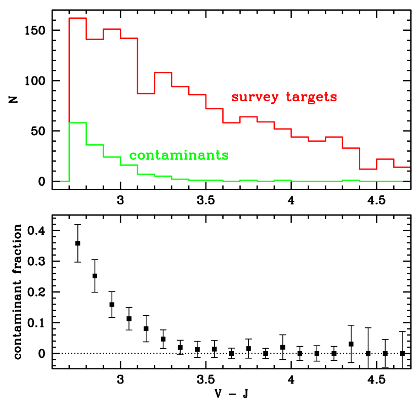
Figure 3.— Histogram of the $V-J$ color distribution of survey stars with spectral morphologies inconsistent with red dwarf of subtype K5 and later (in green). The distribution of $V-J$ colors from the full sample is shown in red. Stars with spectra inconsistent with red dwarfs are close to the blue edge of the survey, which indicates that they are most probably contaminants of the color-magnitude selection, and not the result of mis-acquisition at the telescope.

2.3.1 MDM data

Spectral reduction of the MDM spectra was performed using the CCDPROC and DOSLIT packages in IRAF. Reduction included bias and flatfield correction, removal of the sky background, aperture extraction, and wavelength calibration. The spectra were also extinction-corrected and flux-calibrated based on the measurements obtained from the spectrophotometric standards. We did not attempt to remove telluric absorption lines from the spectra. Many spectra were collected on humid nights or with light cirrus cover, which resulted in variable telluric features. However, telluric features generally do not affect standard spectral classification or the measurement of spectral band indices, since all the spectral indices and primary classification features avoid regions with telluric absorption.

A more common problem at the MDM observatory was slit loss from atmospheric differential refraction. Although this problem could have been avoided by the use of a wider slit, the concomitant loss of spectral resolution was deemed more detrimental to our science goals. Instead, stars were observed as close to the meridian as observational constraints allowed. In some cases, however, stars were observed up to $\pm$2 hours from the meridian, resulting in noticeable slit losses. Fluctuations in the seeing, which often exceeded the slit width, played a role as well. As a result, the spectrophotometric calibration was not always reliable, since the standards were only observed once per night to maximize survey efficiency. Flux recalibration was therefore performed using the following procedure. Spectral indices were measured and the spectra were classified using the classification method outlined below (§3.1). The spectra were then compared to classification templates assembled from M dwarf spectra from the Sloan Digital Sky Survey (SDSS) spectroscopic database. Each spectrum was divided by the classification template of the same alleged spectral subtype. In many cases, the quotients yielded a flat function, indicating that the spectrophotometric calibration was acceptable. Other quotients yielded residuals consistent with first or second order polynomials spanning the entire wavelength range, and indicating problems in the spectrophotometric calibration. A second-order polynomial was fit through the quotient spectra, and the original spectrum was normalized by this fit, correcting for calibration errors. Spectral indices were then measured again, and the spectra reclassified; this yielded changes by 0.5 to 1.0 subtypes for $\approx 20\%$ of the stars (no changes for the rest). The re-normalization was then performed again using the revised spectral subtypes, and the procedure repeated until convergence for all stars.

Finally, all the spectra were wavelength-shifted to the rest frames of their emitting stars. This was done by cross-correlating each spectrum with the SDSS template of the corresponding spectral subtype. Spectral indices were again re-measured, and the stars re-classified. Any change in the spectral subtype prompted a repeat of the flux-recalibration procedure outlined above, and the cross-correlation procedure was repeated using the revised spectral template until converegence.

A sequence of MDM spectra is displayed in Figure 1, which illustrates the wavelength regime and typical quality. Note the telluric absorption features near 6,850Å, 7,600Å, and 8,200Å. Signal-to-noise ratio is generally in the 30$<$S/N$<$50 range near 7500Å.

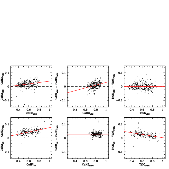
Figure 4.— Comparison between our spectral band index measurements for a subset of 484 stars observed at MDM and UH, and the band index measurements for the same stars as reported in the Palomar-MSU spectroscopic survey of Reid, Hawley, & Gizis (1995). Small but systematic offsets are observed, which are explained by differences in spectral resolution and spectrophotometric calibration between the different observatories. These offsets demonstrate that the spectral indices are instrument-dependent, but that the measurements can be corrected by observing large subsets of stars at the different obervatories. The red segments show the fits to the offsets, which are used to calibrate corrections for each observatory, here using the Palomar-MSU measurements as the standard.

2.3.2 SNIFS data

SNIFS data processing was performed with the SNIFS data reduction pipeline, which is described in detail in Bacon et al. (2001) and Aldering et al. (2006). After standard CCD preprocessing (dark, bias, and flat-field corrections), data were assembled into red and blue 3D data cubes. The data cubes were cleaned for cosmic rays and bad pixels, wavelength-calibrated using arc lamp exposures acquired immediately after the science exposures, and spectrospatially flat-fielded, using continuum lamp exposures obtained during the same night. The data cubes were then sky-subtracted, and the 1D spectra were extracted using a semi-analytic PSF model. We applied corrections to the 1D spectra for instrument response, airmass, and telluric lines based on observations of the Feige 66, Feige 110, BD+284211, or BD+174708 standard stars (Oke et al., 1991). Because the SNIFS spectra are from an integral field spectrograph, operating without a slit, their spectrophotometry is significantly more reliable than the slit-spectra obtained at MDM. In fact, it is possible to perform synthetic photometry by convolving with the proper filter response.

As with the MDM data, SNIFS spectra were shifted to the rest frames of their emitting stars by cross-correlation to SDSS templates (Bochanski et al., 2007) of the corresponding spectral subtype. Spectral indices were re-measured and the stars re-classified. This process was repeated if there was a change in the spectral subtype determination.

A sequence of UH SNIFS spectra are displayed in Figure 2, which show the wavelength range and typical data quality. Signal-to-noise ratio is generally S/N$\approx$100 near 7500Å.

3. Spectral classification

3.1. Visual identification of contaminants

We first examined all the spectra by eye to confirm the presence of morphological features consistent with red dwarfs of spectral subtype K5 and later. The main diagnostic was the detection of broad CaH and TiO moleculars band near 7000Å. Of the 1564 stars observed, 1408 were found to have clear evidence of CaH and TiO. The remaining 156 stars did not show those molecular features clearly, within the noise limit, and were therefore identified as probable contaminants in the target selection algorithm.

Most of these contaminants appeared to be early to mid-type K dwarfs, with a few looking like G dwarfs affected by interstellar reddening. A number of stars also displayed carbon features consistent with low gravity objects, most probably K giants. We suspect that many of the G and K dwarfs have inaccurate V-band magnitudes, making them appear redder than they really are, which would explain their inclusion in our color-selected sample. Interstellar reddening would also explain the inclusion of more distant G dwarfs in our sample, due to their redder colors. An alternate explanation, however, might be that the targets were mis-acquired in the course of the survey, and that the spectra represent random field stars. Indeed the very large proper motion of the sources sometimes makes them difficult to identify at the telescope, as they often have moved significantly from their positions on finder charts. Stars in crowded field are particularly susceptible to this effect. To verify this hypothesis, we compared the $V-J$ color distribution of the contaminants to the distribution of the full survey sample (Figure 3, top panel); the fraction of contaminant stars in each color bin is also shown (bottom panel). The two distributions are significantly different, with the contaminants being dominated by relatively blue stars, and their fraction quickly drops as $V-J$ increases. We can only conclude that the contaminants are not mis-acquired stars, otherwise one would expect the two distributions to be statistically equivalent. Rather, the majority of the contaminants must have been properly acquired and are simply moderately red FGK stars that slipped into the sample in the photometric/proper motion selection, as suggested first.

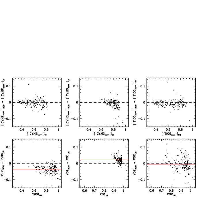
Figure 5.— Comparison between the corrected spectral band index measurements from MDM and the band index measurements of the same stars observed from UH. Observatory-specific corrections to the CaH2, CaH3, and TiO5 indices (see Figure 4) bring the MDM and UH values in close agreement. Small offsets are however observed for the TiO6, VO1, and VO2 indices, which we could not calibrate against Palomar-MSU survey stars. The horizontal red lines show the adopted offsets which are used to correct the MDM values to bring them in line with the UH ones. Offsets are again believed to be due to inter-observatory differences in the spectral resolution and spectrophotometric calibration.

We find an overall contamination rate of $\simeq$10% in our survey, although most of the contamination occurs among stars with relatively blue colors. The contamination rate is $\simeq$26% for red dwarf candidates in the $2.7<V-J<3.0$ color range, but this rate drops to $\simeq$8% for candidates with $3.0<V-J<3.3$, and becomes negligible ($<1\%$) in the redder

$$V-J>3.3$$

candidates. The 156 stars identified as contaminants are included in Table 1 and Table 3 for completeness and future verification. Spectroscopic measurements for these stars, such as band indices, subtypes, and effective temperatures, are however left blank.

3.2. Classification by spectral band indices

3.2.1 M dwarf classification from molecular bandstrengths

The spectra of M dwarfs are dominated by molecular bands from metal oxides (mainly TiO, VO), metal hydrides (CaH, CrH, FeH), and metal hydroxides (CaOH). The most prominent of these in the optical-red wavelength range (5000Å-9,000Å) are the bands from titanium oxide (TiO) and calcium hydride (CaH). The resulting opacities from those broad moleciular bands significantly affect the broadband colors and spectral energy distribution of M dwarfs (Jones, 1968; Allard et al., 2000; Krawchuk, Dawson, & De Robertis, 2000). Early atmospheric models of M dwarfs showed that the strength of the TiO and CaH bands depends on effective temperature, but also on surface gravity and metal abundances (Mould, 1976).

Molecular bands have historically been the defining diagnostic and classification features of M dwarfs. For stars that have settled on the main sequence, one can assume that the surface gravity is entirely constrained by the mass and chemical composition. Leaving only the effective temperature and chemical abundances as general parameters in the classification and/or spectroscopic modeling. For local disk stars of solar metallicity, a classification system representing an effective temperature sequence can thus be established based on molecular bandstrentghs.

The detection and measurement of TiO and CaH molecular bands thus forms the basis for the M dwarf classification system (Joy & Abt, 1974). Molecular bands become detectable starting at spectral subtype K5 and K7, the latest subtypes for K dwarfs (there are no K6, K8, or K9 subtypes). The increasing strength of the molecular bands then defines a sequence running from M0 to M9. The strength of both TiO and CaH molecular bands reach a maximum around $T_{eff}\simeq$2700K. There is a turnaround in the correlation below this point, and molecular bands become progressively weaker at lower temperatures until they vanish (Cruz & Reid, 2002). The reversal and weakening is thought to be due to the condensation of molecules into dust, and their settling below the photosphere (Jones & Tsuji, 1997).

Table 4Coefficients of the spectral index corrections, by observatory.

IDX	$A_{IDX:{\rm PMSU}}$	$B_{IDX:{\rm PMSU}}$	$A_{IDX:{\rm MDM}}$	$B_{IDX:{\rm MDM}}$	$A_{IDX:{\rm UH}}$	$B_{IDX:{\rm UH}}$
CaH2	1.00	0.00	0.95	0.011	0.92	0.004
CaH3	1.00	0.00	0.90	0.070	1.00	-0.028
TiO5	1.00	0.00	1.00	0.000	1.06	-0.063
VO1	$\cdots$	$\cdots$	1.00	0.040	1.00	0.000
TiO6	$\cdots$	$\cdots$	1.00	-0.021	1.00	0.000
VO2	$\cdots$	$\cdots$	1.00	0.005	1.00	0.000

Sequences of classification standards were compiled in (Kirkpatrick, Henry, & McCarthy, 1991), which identified the main molecular bands in the yellow-red spectral regime, where TiO and CaH bandheads are most prominent. To better quantify the classification system, a number of “band indices” were defined by Reid, Hawley, & Gizis (1995), which measure the ratio between on-band and off-band flux, for various molecular bandheads. Calibration of these band indices against classification standards provide a means to objectively assign subtypes based on spectroscopic measurements. Originally, these band indices measured the strengths of various features near $7,000\AA$, where the most prominent CaH and TiO features are found in early-type M dwarfs. These bands, however, become saturated in late-type M dwarfs, which makes their use problematic in later dwarfs. There is a VO band near $7,000$Å, located just between the main CaH and TiO features, which becomes prominent only at later subtypes; and band index measuring this feature was introduced as a primary diagnosis for the so-called “ultra-cool” M dwarfs, and provided a classification scale for subtypes M7-M9 (Kirkpatrick, Henry, & Simons, 1995). Additional band indices associated with TiO and VO bands in the 7500Å-9000Å range, where molecular absorption develops at later subtypes, were introduced as secondary classification features (Lépine, Rich, & Shara, 2003). These form the basis of current classification methods based on optical-red spectroscopy.

Nearby low-mass stars associated with the local halo population have long been known to show peculiar banstrength ratios, and in particular to have weak TiO compared to CaH (Mould, 1976; Mould & McElroy, 1978). A system to identify and classify the metal-poor M subdwarfs based on the strength and ratio of CaH and TiO was introduced by Gizis (1997), and expanded by Lépine, Shara, & Rich (2003) and Lépine, Rich, & Shara (2007), as the spectroscopic census of M subdwarfs grew larger. In this system, the CaH bandstrengths are used as a proxy of $T_{e}ff$ and determine spectral subtypes, while the TiO/CaH band ratio is used to evaluate metallicity. For that purpose, the $\zeta_{TiO/CaH}$ parameter, which is a function of the TiO/CaH band ratio, was introduced by Lépine, Rich, & Shara (2007) as a possible proxy for metallicity, and a tentative calibration with [Fe/H] was presented by Woolf, Lepine, & Wallerstein (2009). One of the main issues in the current M dwarf classification scheme, is that both TiO and CaH bandstrengths are used to determine the spectral subtype, whereas TiO is now believed to be quite sensitive to metallicity. This means, e.g., that moderately metal-rich M dwarfs may be assigned later subtypes than Solar-metallicity ones. In addition, the classification of young field M dwarfs may be affected by their lower surface gravities, which also tend to increase TiO bandstrengths and would thus yield to marginally later subtype assignments compared with older stars of the same $T_{eff}$. These caveats must be considered when one uses M dwarf spectral subtypes as a proxy for surface temperature.

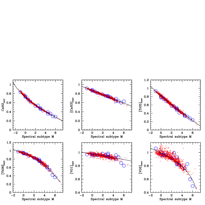
Figure 6.— Variation in the corrected spectral indices as a function of adopted spectral subtypes. The thin black lines show the adopted, revised calibrations for spectral classification. Blue circles represent the subset of classification standards from Kirkpatrick, Henry, & McCarthy (1991) which we observed; the X-axis values of those data points are the formal spectral subtypes adopted in Kirkpatrick, Henry, & McCarthy (1991), while the Y-axis values are the spectral index measurements from our survey. For our own spectral typing scheme, we calculate the average of the subtype values for the ${\rm CaH2}_{c}$, ${\rm CaH3}_{c}$, ${\rm TiO5}_{c}$, and ${\rm TiO6}_{c}$ indices given by the adopted relationships. The two VO indices have relatively weak leverage on early type stars due to the shallow slope in the relationships, and are not used for assigning spectral subtypes of our (mostly early-type) survey stars.

3.2.2 Definition and measurement of band indices

The strength of the TiO, CaH, and VO molecular bands are measured using spectral band indices. These spectral indices measure the ratio between the flux in a section of the spectrum affected by molecular opacity to the flux in a neighboring section of the spectrum minimally affected by molecular opacity. The latter section defines a pseudo-continuum of sorts, although M dwarf spectra do not have a continuum in the classical sense, because their spectral energy distribution strongly deviates from that of a blackbody, and is essentially shaped by atomic and molecular line opacities.

We settle on a set of six spectral band indices: CaH2, CaH3, TiO5, TiO6, TiO7, VO1, and VO2. These band indixes, which we previously used in Lépine, Rich, & Shara (2003) to classify spectra collected at MDM, measure the strength of the most prominent bands of CaH, TiO, and VO in the $6000{\rm\AA}<\lambda<8500{\rm\AA}$ regime. The spectral indices and are listed in Table 2 along with their definition. The CaH2, CaH3, and TiO5 indices are the same as those used in the Palomar-MSU survey, and were first defined in (Reid, Hawley, & Gizis, 1995). The TiO6, VO1, and VO2 indices were introduced by Lépine, Rich, & Shara (2003) to better classify late-type M dwarfs, whose CaH2 and TiO5 indices become saturated at cooler tempratuers and are not as effective for accurate spectral classification of late-type M dwarfs. Each spectral band index is calculated as the ratio of the flux in the spectral region of interest (numerator) to the flux in the reference region (denominator), i.e.:

$$IDX=\frac{\int_{num}I(\lambda)d\lambda}{\int_{denom}I(\lambda)d\lambda}$$ (1)

Because the wavelength range for some indices is relatively narrow (especially the denominator for CaH2, CaH3, and TiO5) it is important that the spectra in which they are measured have their wavelengths calibrated in the rest frame of the star, which is why special care was made to correct all spectra for any significant redshift/blueshift (see above).

Because the measured molecular bandheads are relatively sharp, and because the spectral indices measuring them are defined over relatively narrow spectral ranges, the index values are potentially dependent on the spectroscopic resolution, and may thus depend on the specific instrumental setup used for the observations. In addition, the index values may be affected by systematic errors in the spectrophotometric flux calibration, which can also be dependent on the instrument and/or observatory where the measurements were made. One way to verify these effects is to compare spectral index measurements of the same stars obtained at different observatories. Because of the significant overlap with the Palomar-MSU survey, we can use those stars as reference sample, and recalibrate the spectral indices so that they are consistent to those reported in Reid, Hawley, & Gizis (1995).

Our census have 557 stars in common with the PMSU spectroscopic survey; these stars are all identified with a flag (“P”) in the last column of Table 3. We identify 206 stars from the list observed at MDM and 281 stars from the list observed at UH which have spectral index measurements reported in the PMSU survey. The differences between our measured CaH2, CaH3, and TiO5 and those reported in the PSMU catalog are plotted in Figure 4. Trends and offsets confirm the existence of systematic errors, possibly due to differences in resolution and flux calibration. To verify the spectroscopic resolution hypothesis, we convolved the MDM spectra with a box kernel 5-pixel wide; we found that indeed the MDM indices for the smoothed spectra had their offsets reduced by 0.01-0.02 units, bringing them more in line with the PMSU indices. We also observe that the MDM measurements tend to have a larger scatter than the UH ones; we suggest that this may be due to spectrophometric calibration issues with some of the MDM spectra, as discussed in §2.3.1.

To achieve consistency in the measurements obtained at different observatories, we adopt the values from the PMSU survey as a standard of reference, and calculate corrections to the measurements from MDM and UH by fitting linear relationships to the residuals. A corrections to a spectral band index is thus applied following the general function:

$$IDX_{c}=A_{IDX:OBS}\ IDX_{OBS}+B_{IDX:OBS}\\$$ (2)

where $IDX_{OBS}$ represents the measured value of an index at the observatory $OBS$, and ($A_{IDX:OBS}$,$B_{IDX:OBS}$) are the coefficients of the transformation from the observed value to the corrected one ($IDX_{c}$). Hence the corrected values of the indices CaH2, CaH3 and TiO5 for measurements done at MDM are defined as:

$${\rm CaH2_{c}=A_{\rm CaH2:MDM}CaH2_{\rm MDM}+B_{\rm CaH2:MDM}}$$ (3)

$${\rm CaH3_{c}=A_{\rm CaH3:MDM}CaH3_{\rm MDM}+B_{\rm CaH3:MDM}}$$ (4)

$${\rm TiO5_{c}=A_{\rm TiO5:MDM}TiO5_{\rm MDM}+B_{\rm TiO5:MDM}}$$ (5)

The measurements from the PSMU survey are used as standards for these three indices, and we thus have by definition: $A_{\rm CaH2:PMSU}=A_{\rm CaH3:PMSU}=A_{\rm TiO5:PMSU}=1.0$, $B_{\rm CaH2:PMSU}=B_{CaH3:PMSU}=B_{\rm TiO5:PMSU}=0.0$. For OBS=MDM and OBS=UH, the adopted correction coefficients are listed in Table 4. The corresponding linear relationships are shown as red segments in Figure 4.

To verify the consistency of the corrected spectral band index values, we compare the corrected values for the stars observed at both MDM and UH (the inter-observatory subset). The differences are shown in Figure 5. We find the corrected values CaH2_c, CaH3_c, and TiO5_c to be in good agreement, with no significant offsets beyond what is expected from measurement errors. The corrected values of all three spectral indices are listed in Table 3.

The TiO6, VO1, and VO2 spectral index mesurements from MDM and UH are also compared in Figure 5. Those were not measured in the PMSU survey, since the indices were introduced later (Lépine, Rich, & Shara, 2003), and thus are displayed here without any correction. Small but significant offsets between the MDM and UH values again suggest systematic errors due to differences in spectral resolution and flux calibration. This time we adopt the UH measurements as fiducials, and determine corrections to be applied to the MDM data. The corrections are listed in Table 4 and the corresponding linear relationships are displayed in Figure 5 as red segments. The corrected values of the three spectral indices are also listed in Table 3.

The scatter between the MDM and UH values, after correction, as well as the scatter between the UH/MDM and PMSU values, provide an estimate of the measurment accuracy for these spectral indices. Excluding a few outliers, the mean scatter is $\approx$0.02 units (1$\sigma$) for the CaH2, CaH3, TiO5, TiO6, and VO1 indices, and $\approx$0.04 units for VO2. This assumes that M stars do not show any significant changes in their spectral morphology over time, and that the spectral indices should thus not be variable.

3.2.3 Spectral subtype assignments for K/M dwarfs

Because of the correlation between spectral subtype and the depth of the molecular bands, it is possible to use the values of the spectral band indices to estimate spectral subtypes. This only requires a calibration of the relationship between spectral index values and the spectral subtypes, in a set of stars which were classified by other means, e.g., classification standards. The system adopted in this paper uses the spectral indices listed in Table 2, and follows the methodology outlined in (Gizis, 1997) and (Lépine, Rich, & Shara, 2003). Relationships are calibrated for each spectral index, and spectral subtypes are calculated from the mean values obtained from all relevant/available spectral indices. The mean values are then be rounded to the nearest half integer, to provide formal subtyping with half-integer resolution. The system is extended to late-K dwarfs as well: an “M subtype” with a value $<0.0$ signifies that star is a late-K dwarf: the star is classified as K7 for an index value $\approx-1.0$ and as K5 for an index value $\approx-2.0$ (note: there is no K6 subtype for dwarf stars, and K7 is the subtype immediately preceding M0).

The original spectral-index classification method for M dwarfs/subdwarfs is based on a relationship between subtype and with the CaH2 index, which measures one of the most prominent band at all spectral subtypes, and notably displays the deepest bandhead in metal-poor M subdwarfs Gizis (1997); Lépine, Rich, & Shara (2003). The original relationship is: $\left[SpTy\right]_{CaH2}=10.71-20.63\ {\rm CaH2}+7.91\ \left({\rm CaH2}\right)^{2}$. To verify this relationship, we estimated spectral subtypes from our corrected indices CaH2_c for 16 spectroscopic calibration standards from Kirkpatrick, Henry, & McCarthy (1991), which were observed as part of our survey, and span a range of spectral subtypes from K7.0 to M6.0. We found small but significant differences in our estimated spectral subtypes and the values formally assigned by Kirkpatrick, Henry, & McCarthy (1991); subtypes estimated from the Gizis (1997) relationship tend to systematically underestimate the standard subtypes by $\approx 0.5$ units for stars later than M3. To improve on the index classification method, we performed a $\chi^{2}$ polynomial fit to recalibrate the relationship, obtaining:

$$\left[\rm SpTy\right]_{\rm CaH2}=11.50-21.71\ {\rm CaH2}_{c}+7.99\ \left({\rm CaH2}\right)^{2}$$ (6)

which does correct for the observed offsets at later types. Using this this relatioship as a starting point, and guided by the formal spectral subtype from the classification standards, we performed additional $\chi^{2}$ polynomial fits to calibrate an index-subtype relationships for CaH3:

$$\left[\rm SpTy\right]_{\rm CaH3}=18.80-21.68\ {\rm CaH3}_{c}$$ (7)

Where the corrected values of the spectral bands indices (see Eqs.2-5) are used. The relationships are slightly different from those quoted in Gizis (1997) and Lépine, Rich, & Shara (2003) but are internally consistent to each other, whereas an application of the older relationships to our corrected band index measurements would yield internal inconsistencies, with subtype difference up to 1 spectral subtype between the relationships.

The ratio of oxides (TiO, VO) to hydrides (CaH,CrH,FeH) in M dwarfs is known to vary significantly with metallicity (Gizis, 1997; Lépine, Rich, & Shara, 2007). In the metal-poor M subdwarfs, it is the oxides bands that appear to be weaker, while hydride bands remain relatively strong (in the most metal-poor ultrasubdwarfs, or usdM, the TiO bands are almost undetectable). Therefore it makes sense to rely more on the CaH band as the primary subtype/temperature calibrator. The same $[\rm SpTy]_{\rm CaH2}$ and $[\rm SpTy]_{\rm CaH3}$ relationships should be used to determine spectral subtypes at all metallicity classes (i.e. in M subdwarfs as well as in M dwarfs).

Because the TiO and VO bands are also strong in the metal-rich M dwarfs, it is still useful to include these bands as secondary indicators, to refine the spectral classification. In the late-type M dwarfs, in fact, the CaH bandheads are saturating, and one has to rely on the TiO and VO bands. In fact, the VO bands were originally used to diagnose and calibrate ultracool M dwarfs of subtypes M7-M9 (Kirkpatrick, Henry, & Simons, 1995). The main caveat in using the oxide bands for spectral classification is that this can potentially introduce a metallicity dependence on the estimated spectral subtype, with more metal-rich stars being assigned later subtypes than what they would have based on the strength of their CaH bands alone. In any case, because our sample appears to be dominated by near-solar metallicity stars, we calibrate additional relationships between subtype and the TiO5 and TiO6 bands indices. We first recalculate the subtypes by averaging the values of $\left[SpTy\right]_{CaH2}$ and $\left[SpTy\right]_{CaH2}$, and perform a $\chi^{2}$ fit of the TiO5 and TiO6 indices to the mean subtypews calculated from CaH2 and CaH3, finding:

$$\left[\rm SpTy\right]_{\rm TiO5}=7.83-9.55\ {\rm TiO5}_{c}$$ (8)

$$\left[\rm SpTy\right]_{\rm TiO6}=9.92-15.68\ {\rm TiO6}_{c}+21.23\ \left({\rm TiO6}_{c}\right)^{2}$$

$$-16.65\ \left({\rm TiO6}_{c}\right)^{3}$$ (9)

where again the corrected band indices are used. The relatively sharp non-linear deviation in the TiO6 distribution around M3 forces the use of a third order polynomial in the fit.

We also determine the relationships for the VO1 and VO2 band indices. This this after recalculating the subtypes from the average of $\left[\rm SpTy\right]_{\rm CaH2}$ and $\left[\rm SpTy\right]_{\rm CaH2}$, $\left[\rm SpTy\right]_{\rm TiO5}$, and $\left[\rm SpTy\right]_{\rm TiO6}$, a $\chi^{2}$ fit again yields:

$$\left[\rm SpTy\right]_{\rm VO1}=69.8-71.4\ {\rm\left[\rm VO1\right]_{c}}$$ (10)

$$\left[\rm SpTy\right]_{\rm VO2}=9.56-12.47\ {\rm\left[\rm VO2\right]_{c}}+22.33\ \left({\rm\left[\rm VO2\right]_{c}}\right)^{2}$$

$$-19.59\ \left({\rm\left[\rm VO2\right]_{c}}\right)^{3}.$$ (11)

The VO indices however make relatively poor estimators of spectral subtypes for our sample, mainly because the shallow slope at earlier subtypes provides little leverage. The VO2 index also shows unexpectedly large scatter in the MDM spectra, including in the classification standard stars, which we suspect is due the fact that the index is defined very close to the red edge of the MDM spectral range and is thus more subject to statistical noise and flux calibration errors. We therefore do not include $\left[SpTy\right]_{VO12}$ and $\left[SpTy\right]_{VO2}$ in the final determination of the spectral subtypes.

Table 5Distribution by spectral subtype of the 1564 survey stars

Spectral subtype	N
G/K	160
K7.0	27
K7.5	101
M0.0	177
M0.5	160
M1.0	152
M1.5	147
M2.0	141
M2.5	119
M3.0	125
M3.5	125
M4.0	72
M4.5	36
M5.0	13
M5.5	4
M6.0	2
M6.5	2
M7.0	1

Fig. 6 plots all the corrected spectral band indices as a function of the adopted spectral subtype. The relatively small scatter ($\approx 0.02$) in the distribution of $\left[\rm CaH2\right]_{c}$, $\left[\rm CaH3\right]_{c}$, $\left[\rm TiO5\right]_{c}$ and $\left[\rm TiO6\right]_{c}$ demonstrate the internal consistency of the spectral type calibration for the four indices. All four relationships have an average slope $\approx 10$, which means that since those indices have an estimated measurement accuracy of $\approx 0.02$ units, the spectral subtypes calculated by combining the four indices should be accurate to about $\pm 0.10$ subtype assuming that the measurement errors in the four indices are uncorrelated. While this would make it possible to classify the stars to within a tenth of a subtype, we prefer to follow the general convention and assign spectral subtypes to the nearest half integer.

To verify the consistency of the spectral classification, we compare the spectral types evaluated independently for the list of 141 stars observed at both MDM and UH. We find that 82% of the stars end up with the same spectral type assigments from both observatories, i.e. they have spectra assigned to the same half-subtype. All the other stars have classifications within 0.5 subtypes. This is statistically consistent with a $1\sigma$ error of $\pm$0.18 on the spectral type determination, slightly larger than the assumed $0.1$ subtype precision estimated above. This suggests a $3\sigma$ error of about $\pm$0.5, which justifies the more conservative use of half-subtypes as the smallest unit for our classification.

The resulting classifications based on the CaH and TiO band index measurements are listed in Table 3. The numerical spectral subtype measured from the average of the band indices is listed to 2 decimal figures. These values are rounded to the nearest half integers to provide our more formal spectral classifications to a half-subtype precision. The non-rounded values are however useful for comparison with other physical parameters as they provide a continuous range of fractional values; these fractional subtype values are used in the analysis throughout the paper

A histogram of the distribution of spectral subtypes is shown in Figure 7, with the final tally compiled in Table 5. Most of the stars in our survey have subtypes in the M0.0-M3.0 range. The sharp drop for stars of subtypes K7.5 and K7.0 is explained by the color selection used in the Lépine & Gaidos (2011) catalog ($V-J>2.7$) which was originally intended to select only M dwarfs; note that stars with subtypes earlier than K7.0 are also excluded from the graph, and are probably contaminants of the color selection in any case. Our deficit of K7.0 and K7.5 stars however spectra demonstrates that the adopted selection criterion is efficient in excluding K dwarfs from the catalog. The distribution of spectral subtypes also shows a marked drop in numbers for subtypes M4 and later. This is a consequence of the relatively bright magnitude limit ($J<9$) of our subsample, combined with the low absolute magnitudes of late-type M dwarfs, which excludes most late-type stars from our survey, since these tend to be fainter than our magnitude limit, even relatively nearby ones.

Figure 7.— Distribution of spectral subtype M, for the stars in our survey, with K5=-2 and K7=-1. Most stars are found to be early-M objects. The sharp drop at subtypes K7.5 and earlier is a consequence of our initial $V-J>2.7$ color cut, which was meant to select only stars cool enough and red enough to be M dwarf. The sharp drop for subtypes M4 and later is a consequence of the high magnitude limit ($J<9$) of our survey, which restricts the distance range over which late-M stars are selected. The magnitude limit also explains the slow drop in numbers from subtypes M0 to M3, whereas one would normally expect the lower-mass M3 stars to be more common than earlier-type objects in a volume limited sample.

3.3. Semi-automated classification using THE HAMMER

Figure 8.— Comparison of spectral types assigned by the spectral index method and those assigned by the Hammer code, which is used for stellar classification in the Sloan Digital Sky Survey. Subtypes generally agree to within the advertized precision of the Hammer ($\pm$1 subtype, illustrated by the slanted lines), although the Hammer subtypes are marginally later than the spectral index subtypes, by 0.27 subtype on average.

To verify the accuracy and consistency of spectral typing based the spectral-index method described above, we performed independent spectral classification using the Hammer code (Covey et al., 2007). The Hammer was designed to classify stars in the Sloan Digital Sky Survey Spectroscopic database, including M dwarfs (West et al., 2011). The code works by calculating a variety of spectral-type sensitive band indices, and uses a best-fit algorithm to identify the spectral subtype providing the best match to those band indices. For late-K and M dwarfs, spectral subtypes are determined to within integer value (K5, K7, M0, M1, …, M9).

However, to ensure that the automatically determined spectral types were accurate we used the manual “eye check” mode of the Hammer (version 1.2.5). This mode is typically used to verify that there are no incorrectly typed interlopers. The Hammer allows the user to compare spectra to a suite of template spectra to determine the best match. West et al. (2011) have found that for late-type M dwarfs, the automatic classifications were systematically one subtype earlier than those determined visually. Our analysis confirms this offset, and we therefore disregarded the automatically determined Hammer values to adopt the visually determined subtypes.

The resulting subtypes are listed in Table 3. Some 170 stars were not found to be good fits to any of the K5, K7, or M type templates, and thus identified as early-K or G dwarfs. This subset includes all of the 156 stars that were visually identified as non-M dwarfs on first inspection (see §3.1). The remaining 14 stars were initially found to be consistent with late-K stars, and classified as K7.0 and K7.5 objects using the spectral index method described in §3.2 above; we investigated further to determine why the stars were classified as early K using the Hammer. On closer inspection, we found that 3 of the stars are indeed more consistent with mid-K dwarfs that K7.0 or K7.5, and we thus overran the spectral index classification and reclassified them as ”G/K” in Table 3. For the other 11 stars flagged as mid-K type with the Hammer, we determined that the stars do show significant evidence for TiO absorption, which warrants that the stars retain their spectral-index classifiction of K7.0/K7.5.

In the end Table 3 lists 159 stars from our initial sample that are identified and early-type G and K dwarf contaminants, and most likely made our target list due to inaccurate or unreliable $V-J$ colors. The remaining 1405 stars are formally classified as late-K and M dwarfs.

A comparison of spectral subtypes determined from the spectral-index and Hammer methods is shown in Figure 8. Because the Hammer yields only integer subtypes, we have added random values in the $-0.4,0.4$ range to facilitate the comparion. Slanted lines in Figure 8 show the range expected if the two classification methods (spectral index, Hammer) agree to within 1.0 subtypes. There is however a mean offset of 0.26 subtypes between the spectral index and Hammer classifications, with the Hammer subtypes being on average slighlty later.

Figure 8 also reveals a number of outliers with large differences in spectral subtypes between the two methods. We found 48 stars with differences in spectral subtyping larger than $\pm$1.5. The spectra from these stars were examined by eye: except for one star, we found the band-index classifications to agree much better with the observed spectra than the Hammer-determined subtypes. The one exception is the star PM I11055+4331 (Gl 412B) which the band index measurements classify as M6.5; in this case the Hammer determined subtype of M 5.0 appears to be more accurate. This exception likely occurs because of the saturation of the CaH2 and CaH3 subtypes in the late-type star, which make the band-index classification less reliable.

3.4. Comparison with the “Meet the Cool Neighbors” survey

Figure 9.— Comparison of spectral types assigned by our spectral index method and those assigned in the ”Meet the Cool Neighbors” (MCN) spectroscopic follow-up program. This shows all 161 stars in common between our survey and the MCN program. Spectral index subtypes are show before rounding up to the nearest half-integer; the MCN subtypes have random values of $\pm$0.2 to help in the comparison. The classifications generally agree to within $\pm$0.5 subtypes (slanted lines). Our subtypes are however marginally later (by 0.28 subtypes on average) than the MCN subtypes.

After the PMSU survey, the largest spectroscopic survey of M dwarfs in the northern sky was the one presented in the “Meet the Cool Neighbors” (MCN) paper series (Cruz & Reid, 2002; Cruz et al., 2003; Reid et al., 2003, 2004; Cruz et al., 2007; Reid, Cruz, & Allen, 2007). In this section we compared the spectral clssification from the MCN survey with our own spectral type assignments.

To identify the stars in common between the two surveys, we first performed a cross-correlation of the celestial coordinates of the stars listed in the MCN tables, to the coordinates listed in the SUPERBLINK catalog. This was performed for the 1077 stars in MCN which are north of the celestial equator. We found counterparts in the SUPERBLINK catalog to within 1″for 860 of the MCN stars. Of the 217 MCN stars with no obvious SUPERBLINK counterparts, 148 are classified as ultracool M dwarfs (M7-M9) or L dwarfs (L0-L7.5) which means they are very likely missing from the SUPERBLINK catalog because they are fainter than the V=19 completeness limit of the catalog. Of the 71 remaining stars, close examination of Digitized Sky Survey scans failed to identify the stars at the locations quoted in MCN. A closer examination of the fields around those stars identified 49 cases where a high proper motion stars could be found within 3′of the quoted MCN positions. These nearby high proper motion stars are all listed in SUPERBLINK, and have colors consistent with M dwarfs; we therefore assumed that the quoted MCN positions are in error, and matched those 49 MCN entries with the close by high proper motions stars from SUPERBLINK. Of the remaining 22 stars we found 6 that have proper motions below the SUPERBLINK limit of $\mu>40$ mas yr^-1 and another 5 stars with proper motions within the SUPERBLINK limit but that appear to have been missed by the SUPERBLINK survey. Finally, there were 11 MCN stars that we could not identify at all on the Digitized Sky Survey images, and we can only assume that the positions quoted in MCN are too large for proper identification, and that the stars should be considered “lost”.

Of the 909 stars in the MCN program with SUPERBLINK counterparts, we found only 219 which satisfy the magnitude limit ($J<9$) of our present sample of very bright M dwarfs. Of those, 52 stars have colors bluer ($V-J<2.7$) than our sample limit; 48 of them are classified as F and G stars in MCN, consistent with their bluer colors. The other 4 stars are classified as M dwarfs, although they have $V-J<2.7$ according to Lépine & Gaidos (2011). We infer that our $V-J$ colors for those stars are probably underestimated, which suggests that our color selection may be overlooking a small fraction of nearby M dwarfs. In addition, we found another 6 stars which have $V$ magnitudes and $V-J$ colors within our survey range, but were rejected by the additional infrared ($J-H$,$H-K$) color-color cuts used in Lépine & Gaidos (2011) to filter out red giants. All 6 stars are very bright in the infrared, and it appears that at least one of the $H$ or $K$ magnitudes listed in the 2MASS catalog may be in error, making the stars appear to have $J-H$ and/or $H-K$ colors more consistent with giants. Four of the stars are classified as M dwarfs in MCN, the other two are late-K dwarfs. Overall, this makes a total of 8 M dwarfs from the MCN census that were overlooked in our selection out of the MCN subset of $\approx$150 nearby M dwarfs. This suggests that our color cuts, combined with magnitude measurement errors, might be missing $\sim 5\%$ of the very bright, nearby M dwarfs.

In the end, this leaves only 161 stars in common between the MCN program and our own spectroscopic survey. The stars are all classified as late-K and M dwarfs by MCN, with subtypes ranging from K5 to M5.5. All 159 stars are identified with a flag (”M”) in the last column of Table 3; we note that 82 of these stars were also observed as part of the PMSU survey. We compare the spectral type assignments from both surveys in Figure 9, where the M dwarf subtypes from MCN are plotted against the (non-rounded) subtypes calculated from the spectral-band indices. To ease the comparison, random values of $\pm$0.2 are added to the MCN subtypes. Overall, our classifications agree to within $\pm$0.5 subtypes with the MCN values. The MCN subtypes, however, tend to be marginally earlier on average, by 0.28 subtypes; this is in contrast with the Hammer classifications (see above) which tend to be slightly later than our own. For the MCN subtypes, the effect is more pronounced for the earlier M dwarfs ($<$M2.5), where the mean offset is 0.43 subtypes, whereas the mean offset is only 0.09 for the later stars.

To investigate the difference in spectral subtype assignments, we compare the recorded values of the CaH2, CaH3, and TiO5 indices between the MCN program and our own survey. After a search of the various tables published in the MCN series of papers, we identified 54 stars in common between the two programs, and for which values of CaH2, CaH3, and TiO5 were also recorded in both. The differences between the spectral index values are shown in Figure 10. For our own survey, the corrected values of these indices are used, i.e. CaH2_c, CaH3_c, and TiO5_c as defined in §3.2.2. We find that the CaH2 and TiO5 are estimated marginally higher in the MCN program than they are in our survey, and this very likely explains the difference in spectral typing: the higher index values yield margnially earlier spectral subtypes. This again emphasizes the variation in the spectral index measurements due to spectral resolution and other instrumental setups, and the need to apply systematic corrections between observatories to obtain a uniform classification system.

Figure 10.— Differences between the spectral index values recorded in the “Meet the Cool Neighbors” (MCN) program and those measured in the present survey. The values are compared for a subset of 55 stars in common between the two surveys and for which values of CaH2, CaH3, and TiO5 were recorded. For the present survey, we use the corrected values (CaH2_c, CaH3_c, and TiO_c) as defined in §3.2.2. The MCN values tend to be marginally higher on average, especially for stars of earlier spectral subtypes. This explains the marginally earlier spectral subtype assigments in MCN compared with the ones presented in this paper (see Figure 9).

We note that smaller subsets of stars in our census may also have spectroscopic data published in the literature, from various other sources. This is especially the case for the 102 stars from the CNS3 and stars with very large proper motions $mu>0.2\arcsec$ yr^-1 which have been more routinely targeted for follow-up spectroscopic observations. Additional pectroscopic surveys of selected bright M dwarfs include, Scholz et al. (2002), Scholz et al. (2005), Reyle et al. (2006), and (Riaz, Gizis, & Harvin, 2005), which all have a few stars in common with our catalog. Other surveys of nearby M dwarfs have mainly been targeting fainter stars (Bochanski et al., 2005, 2010; West et al., 2011), and do not overlap with our present census.

3.5. Color/spectral-type relationships

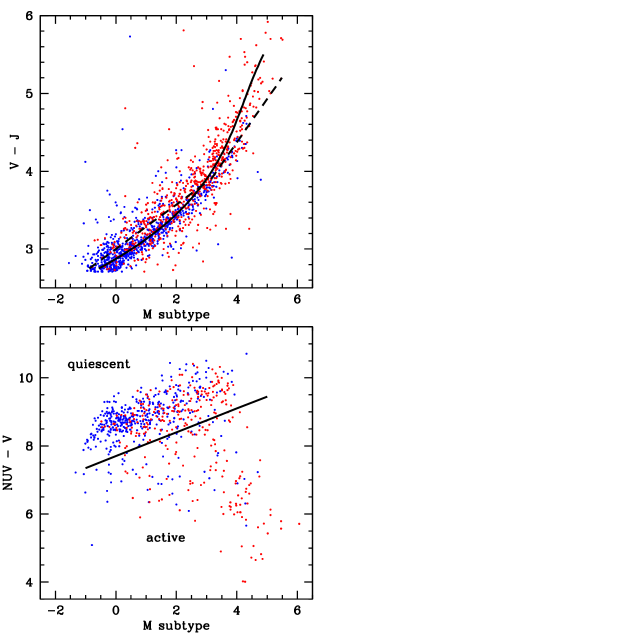
Figure 11.— Variation of the UV-to-optical $NUV-V$ color index and the optical-to-IR $V-J$ color index as a function of spectral subtype M. Stars with more reliable V magnitudes from the Tycho-2 catalog are shown in blue, stars with V magnitudes derived from less reliable photometric measurements are shown in red. The distribution of ultra-violet to optical colors ($NUV-V$) with spectral subtype shows two populations, one with a tight correlation, consistent with blackbody distribution and labeled “quiescent”, and a scattered population of stars with clear $UV$ excess, labeled “active”. The distribution of $V-J$ with subtype closely follows the relationship used by Lépine & Gaidos (2011) to predict subtypes from $V-J$ colors (dashed line) except for stars of later subtypes which have redder colors than predicted. A revised relationship (full line) is fitted to the data. Outliers point to stars with bad $V$ magnitude measuremens.

Table 6Colors and $T_{eff}$ for red dwarfs in our survey as a function of spectral subtype.

subtype	nNUV-V	$\overline{NUV-V}$	$\sigma_{NUV-V}$	nV-J	$\overline{V-J}$	$\sigma_{V-J}$	$\overline{T_{eff}}$	$\sigma_{T_{eff}}$
K 7.0	11	8.17	0.21	25	2.90	0.31	4073	98
K 7.5	47	8.60	0.31	97	2.89	0.16	3883	82
M 0.0	87	8.66	0.36	175	2.94	0.21	3762	71
M 0.5	79	8.74	0.30	159	3.11	0.34	3646	48
M 1.0	76	8.89	0.39	151	3.19	0.18	3565	44
M 1.5	57	9.07	0.38	147	3.36	0.23	3564	39
M 2.0	57	9.25	0.47	139	3.52	0.34	3518	57
M 2.5	48	9.45	0.50	118	3.69	0.28	3500	61
M 3.0	34	9.61	0.38	125	3.91	0.28	3423	62
M 3.5	28	9.69	0.33	124	4.17	0.33	3320	66
M 4.0	5	9.72	0.35	71	4.45	0.41	3204	76
M 4.5	1	$\cdots$	$\cdots$	36	4.81	0.46	3119	43
M 5.0	0	$\cdots$	$\cdots$	12	5.23	0.50	3014	61

Spectral subtypes were inititially estimated in Lépine & Gaidos (2011) based on $V-J$ colors alone. Here we verify this assumption and re-evaluate the color-magnitude relationship for bright M dwarfs. The $V-J$ color index combines estimated optical ($V$) magnitudes from the SUPERBLINK catalog to the infrared $J$ magnitudes of their 2MASS counterparts. The SUPEBLINK $V$ magnitudes are estimated either from the Tycho-2 catalog $V_{T}$ magnitudes, or from a combination of the Palomar photographic $B_{J}$ (IIIaJ), $R_{F}$ (IIIaF), and $I_{N}$ (IVn) magnitudes, as described in Lépine & Shara (2005). Values of $V$ are more accurate for the former ($\approx$0.1mag) than for the latter ($\gtrsim$0.5mag); Table 1 indicates the source of the V magnitude.

Mean values and dispersion about the mean of the $V-J$ colors are listed in Table 6, for each bin of half-integer subtype; the table also lists how many stars of each type are in each bin. The $V-J$ colors of our stars are also plotted as a function of spectral subtype in Figure 11 (top panel). The adopted color-subtype relationship from Lépine & Gaidos (2011) is shown as a thick dashed line in Figure 11. Stars with the presumably more reliable Tycho-2 magnitudes are shown in blue, while stars with photographic $V$ magnitudes are shown in red. Stars with Tycho-2 $V$ magnitudes appear to have marginally bluer colors at a given subtype; this however is an effect of the visual magnitude limit of the Tycho-2 catalog, which includes only the brightest stars in the $V$ band and is thus more likely to list bluer objects. The Lépine & Gaidos (2011) relationship generally follows the distribution at all subtypes, but with mean offsets up to $\pm$0.4mag in $V-J$, especially at earlier and later subtypes. We perform a $\chi^{2}$ fit to determine the following, improved relationship:

$$\left[\rm SpTy\right]_{V-J}={\rm-32.79+20.75(V-J)-4.04(V-J)^{2}}$$

$${\rm+0.275(V-J)^{3}}$$ (12)

after exclusion of 3-$\sigma$ outliers. The relationship is shown in Figure 11 (solid line). There is a scatter of 0.7 subtype between $\left[SpTy\right]_{V-J}$ and the subtype determined from spectral band indices. While the spectroscopic classification is more accurate and reliable, photometrically determined spectral subtypes using the equation above should still be accurate to $\pm$0.5 subtype about 80% of the time, and to $\pm$1.0 subtype 95% of the time, which may be useful for a quick assessment of subtype when spectroscopic data is unavailable.

We also compare the near-UV to optical magnitude color $NUV-V$ for the 714 stars in our sample which have counterparts in GALEX; the distribution is shown in Figure 11 (bottom panel). We find that stars become progressively redder as spectral subtype increases, from $NUV-V=8$ at M0 to $NUV-V=10$ at M4. There is however a significant fraction of M dwarfs which display much bluer $NUV-V$ colors at any given subtype. The excess in $NUV$ flux is strongly suggestive of chromospheric activity (see §6 below for a more detailed analysis). We separate the active stars from the more quiescent objects with the following condition:

$$\left[\rm NUV-V\right]>7.7+0.35\left[\rm Spty\right]\$$ (13)

where $\left[\rm Spty\right]$ is the mean spectral subtype calculated from equations 8-11. After excluding active stars, we calculate the mean values and scatter about the mean of $NUV-V$ for each half-integer spectral subtype. Again those are listed in Table 6 for reference; the table also lists the number of non-active stars used to calculate the mean. There is not a sufficient number of stars to calculate mean values and scatter at M4.5 (1 star) and M5.0 (0 star).

4. Survey completeness

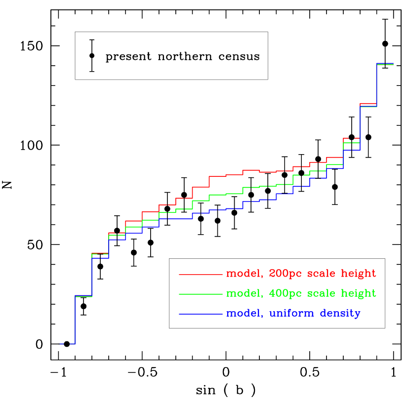
Figure 12.— Number of spectroscopically confirmed M dwarfs as a function of $sin(b)$, where $b$ is the Galactic latitude. Numbers from our census are shown as filled circles, with errorbars showing the Poisson noise. Distributions predicted from models with either uniform space density, or with decreases perpendicular to the Galactic plane following scale-heights of 200pc and 400pc, are shown for comparison. The observed distribution is largerly consistent with a uniform density in the local $d<70$pc volume, with no evidence for incompleteness at low Galactic latitude.

Our 1,564 spectroscopically confirmed M dwarfs are drawn from a catalog with proper motion limit $\mu<40$ mas yr^-1. The low proper motion limit of the SUPERBLINK catalog catches most of the nearby stars, but potentially overlooks nearby M dwarfs with small components of motion in the plane of the sky – either due to low space motion relative to the Sun or to projection effects. The catalog may also be affacted by other sources of incompleteness (e.g. missed detection, faulty magnitude estimate) which means that at least some very bright, nearby M dwarfs must be missing from our survey due to kinematics bias and other effects.

To evaluate the completeness of our census, we first consider the primary source of incompleteness: the kinematics bias of the proper motion catalog. As discussed in Lépine & Gaidos (2011), the completeness depends on the local distribution of stellar motions, and increases with distance from the Sun. To estimate the kinematics bias in our sample, we built a model reproducing the local distribution and kinematics of nearby M dwarfs. We first assumed the stars to have a uniform spatial distribution in the solar vicinity, and generated a random distribution of $10^{5}$ objects within a sphere of radius $d=70$pc centered on the Sun. We assigned transverse motions to all the stars, assuming a velocity-space distribution similar to that of the nearby (d$<$100pc) G dwarfs in the Hipparcos catalog (van Leeuwen, 2007). Because the distribution of stellar velocities is not isotropic, we assigned transverse motions for each simulated star based on the statistical distribution of transverse motions for Hipparcos stars with sky coordinates within $30^{deg}$ of the simulated object. We also used the simplifying assumption that the local M dwarf population has a uniform distribution of absolute magnitudes over the range $5<M_{J}<15$, which is the approximate range of absolute magnitudes reported in the literature for M dwarfs.

We then counted the total number of stars in the simulation with apparent magnitudes $J<9$, and calculated the fraction of those stars with proper motions $\mu>40$ mas yr^-1. We found that 93% of nearby M dwarfs with $J<9$, on average, have proper motions above the SUPERBLINK limit. M dwarfs with $J<9$ extend to a maximum distance of 63 parsecs; most of the stars which fail the proper motion cut are in the higher distance range (d$<$50pc), and are stars near the bright end of the luminosity distribution $M_{J}\approx 5-6$. For this reason, if we assume a luminosity function which increases at fainter absolute magnitudes, the fraction of $J<9$ stars which fall within the proper motion cut is increased, because more of the $J<9$ stars in the local population are now M dwarfs of lower luminosities and closer distances, which are more likely to have high proper motions. The observed field M dwarf luminosity function does indeed increase for early-type dwarfs, to reach a peak at $M_{J}\simeq 8.0$ (Reid, Gizis, & Hawley, 2002; Bochanski et al., 2010), which means that the 93% completeness estimated above must be a lower limit. To verify this, we tested a luminosity function where the number of stars increases linearly with absolute magnitude and doubles from $M_{J}=5$ to $M_{J}=8$; with this model, our simulations showed that 96% of all $J<9$ M dwarfs, would have $\mu>40$ mas yr^-1, and thus be within the detection limit of SUPERBLINK. Overall, this suggests that only about $5\%$ of all $J<9$ M dwarfs on the sky will be overlooked in our census because of the proper motion bias.

The SUPERBLINK surveys does however suffer from various other sources of incompleteness, such as the inability to detect moving stars in saturated regions of photographic plates (i.e. in the immediate vicinity of very bright stars), or a difficulty in detecting stars in very crowded field. Also, the SUPERBLINK code has trouble detecting the motions of relatively bright $V<12$ stars because of the saturated cores of their point spread functions. In practice, this is mitigated by incorporating data from the Tycho-2 catalog, which provides very accurate proper motion measurements for bright stars. However the Tycho-2 catalog itself has some level of incompleteness in the $8<V<12$ manitude range.

One way to test incompleteness due to crowding or saturation is to examine the distribution of SUPERBLINK stars as a function of Galactic latitude. Crowding and saturation effects should be more pronounced in low Galactic-latitude fields, where the stellar density is high. In comparison, stars in high Galactic latitude fields will be easier to detect with the SUPERBLINK code. The same is true for the Tycho-2 catalog, which should be more complete at high Galactic latitudes.

We calculated the number of spectroscopically confirmed M dwarfs in our sample as a function of $sin(b)$, where $b$ is the Galactic latitude. The distribution is shown in Figure 12; the number of stars in each bin is plotted as a filled circle, with errobars showing the $1\sigma$ Poisson error. The distribution increases with $sin(b)$ because our stars are all located north of the celestial equator. For comparison, we plot the trend expected of a uniform distribution of stars in the local volume (blue histogram), assuming the same total number of stars as in our census. We find our data to be largely consistent with the uniform distribution model, and see no evidence of a significant dip at low Galactic latitude, which one would expect if the SUPERBLINK survey is incomplete at low $b$. This suggests that our sample does not suffer from significant sources of incompleteness due to saturation/crowding.

One might however argue that the uniform density assumption is invalid for a census extending to $\simeq$70pc of the Sun, and that a slight overdensity of stars should be detected at low Galactic latitudes. The fact that we see no evidence of such an overdensity in our data would then be indirect evidence of incompleteness at low Galactic latitude. To examine this possibility, we estimated the expected distributions from simulations in which the stellar density perpendicular to the plane (i.e. along $Z$) decreases with scale heights of 400pc or 200pc. Kinematics and absolute magnitude distributions were also simulated as described above, and stars were selected based on $J<9$ and $\mu>40$ mas yr^-1. The mean distributions from the 400pc and 200pc scale-height models are shown in Figure 12, and do indeed predict a slight overdensity of objects at low Galactic latitudes. Assuming that all the stars at high Galactic latitude are detected in all the models, we find a $\sim$5% excess of stars in the 400pc scale-height model over the observed number, and a $\sim$10% excess of stars in the 200pc scale-height model. One might then argue that the SUPEBLINK census potentially has an additional 5%-10% incompleteness level, due to incompleteness in the plane of the Milky way. This is most probably an overestimate, however, because there is no evidence that the local stellar distribution shows any significant decrease with $Z$. Overall, the SUPERBLINK census appears to be essentially complete at low Galactic latitudes.

Proper-motion selection may introduce an additional bias against metal-rich and/or young stars, which tend to have lower components of motion in the vicinity of the Sun. However this effect is expected to be small, e.g. a few percent against [Fe/H] = 0 relative to [Fe/H] = -0.5 at 45 pc (Gaidos et al., 2012). Nearly all likely members of the Hyades (Perryman et al., 1998), Ursa Majoris (King et al., 2003), and TW Hydrae (Reid, 2003) young nearby moving groups have proper motions that exceed 40 mas yr^-1 and thus would not be selected against using the current selection method.

Finally, some bright M dwarfs may be overlooked because of the imposed color cuts, due to magnitude errors and uncertainties. As described in §3.4 above, a handful of previously known M dwarfs from the MCN census were overlooked in our target selection for precisely those reasons. As suggested in §3.4, it is possible that we may be overlooking 5% of bright M dwarfs because of magnitude errors. This, combined with the estimated 96% completeness in the proper motion selection estimated above, suggests that our list of 1405 M dwarfs likely includes $\approx 91\%$ of all existing M dwarfs with infrared magnitude $J<9$ as seen from Earth. There may still be $\approx$140 bright M dwarfs to be identified, although the precise number can only be determined after these “missing” stars are found.

5. Phoenix Model fits and $T_{eff}$ estimates

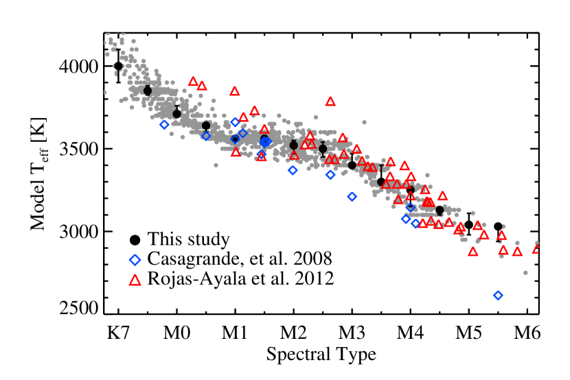
Figure 13.— Effective temperatures for the bright M dwarfs in our survey determined by fits to the PHOENIX models. The gray points represent individual objects, while the large black points are the median values of the objects within each half subtype bin. The error bars are the interquartile ranges. Blue diamonds and red triangles show the T_eff estimates for subsets of stars in our survey whose tempreatures were estimated from photometry Casagrande, Flynn, & Bessell (2008) and model fits to infrared spectra (Rojas-Ayala et al., 2012) respectively. While both spectroscopic estimates show evidence of a plateau at M2-M3, the photometric estimates do not concur.

We compared our spectra to a grid of 298 models of K- and M-dwarf spectra generated by the BT-SETTL version of PHOENIX (Allard et al., 2010). BT-SETTL includes updated opacities (i.e. of H₂O), revised solar abundances (Asplund et al., 2009), a refractory cloud model, and rotational hydrodynamic mixing. The models include effective temperatures $T_{eff}$ of 3000-5000 K in steps of 100 K, $\log g$ values of 4, 4.5, and 5, and metallicities of [M/H] = -1.5, -1, -0.5, 0, +0.3, and +0.5. For each temperature, $\log g$ and metallicity value, we selected the model with $\alpha$/Fe that was closest to solar.

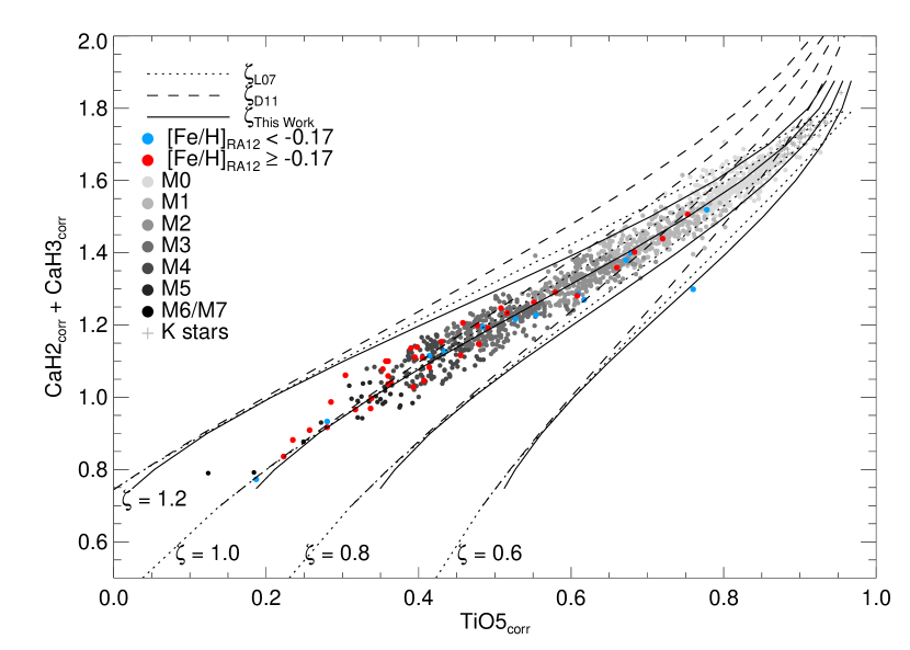
Figure 14.— Distribution of corrected CaH2+CaH3 vs TiO5 band index values for the stars in our survey (grey dots - with brightness levels correlating with spectral subtype). There is a tight correlation between the two indices, which are both also correlated with spectral subtypes, with earlier stars on the upper right of the diagram as shown. The distribution is used as a guide to calibrate the value of $\zeta$, with $\zeta=1$ assumed to trace the CaH2+CaH3/TiO5 relationship for stars with average Galactic disk abundances (near-solar). The iso-$\zeta$ contours from the earlier calibrations of Lépine, Rich, & Shara (2007) and Dhital et al. (2012) are shown as dotted and dashed lines, respectively. When applied to our corrected spectral index values, they both diverge from the observed distribution at earlier subtypes, with the Lépine, Rich, & Shara (2007) overestimating the $\zeta$ of late-K and early-M dwarfs, while the Dhital et al. (2012) calibration yield underestimates. This emphasizes again the need to use properly recalibrated and corrected spectral index values (see Figures 4-5). Our revised, dataset-specific calibration is shown with the continuous lines. Known metal-rich amd metal-poor stars are denoted in red and blue, respectively.

The spectral density of model calculations varies with wavelength but is everywhere vastly greater than the resolution of our spectra. Model spectra were thus convolved with a gaussian with FHWM of the same resolution as the spectra, and a corrective shift (typically less than a resolution element) was found by cross-correlating the observed and model spectra. Normalized spectra were ratioed and $\chi^{2}$ calculated using the variance spectrum of the observations. We restricted the spectral range over which $\chi^{2}$ is calculated to 5600-9000Å and excluded the problematic region 6400-6600Å which contains poorly-modeled TiO absorption (Reyle et al., 2011). We also excluded regions where the telluric correction is rapidly changing with wavelength, i.e. the slope, smoothed over 4 resolution elements or 11.7Å, exceeds 1.37 Å^-1. The model with the smallest $\chi^{2}$ value was identified. For a more refined estimate of effective temperature, we selected the 7 best-fit models and constructed 10,000 linear combinations of them; the “effective temperature” of each is the weighted sum of the temperatures of the components. We again found the model with the minimum $\chi^{2}$. We calculated the standard deviation of $T_{eff}$ among the combination models as a function of the maximum allowed $\chi^{2}$. We reported the maximum standard deviation as a conservative estimate of uncertainty. We also calculated formal 95% confidence intervals for $T_{eff}$ based solely on the expected distribution of $\chi^{2}$ for $N-3$ degrees of freedom, where $N\sim 1100$ is the number of resolution elements used in the fit. The parameters of the best-fit model, and the refined $T_{eff}$, standard deviation, and confidence intervals are reported in Table 3.

Values of $T_{eff}$ calculated for individual stars are plotted in Figure 13 as a function of their spectral subtype (grey dots). Median values for stars within each half-subtype bin are plotted in black, with error bars showing the interquartile ranges. Our model-fit algorithm prefers values that match the $T_{eff}$ model grid, which have a 100K grid step (i.e., 3500K is preferred over 3510K).

Our results suggest the existence of a $T_{eff}$ plateau spanning M1-M3. To investigate this further, we compare our values to the effective temperatures reported in Casagrande, Flynn, & Bessell (2008) for 18 of the stars in our sample, and in (Rojas-Ayala et al., 2012) for another 49 stars; our own spectral type determinations are combined to the T_eff measured by the other authors. The values are compared in Figure 13. We find that our mid-type plateau is corroborated with the (Rojas-Ayala et al., 2012) values, but not with those from Casagrande, Flynn, & Bessell (2008), whose values decrease more linearly with spectral subtype. The effective temperatures in Casagrande, Flynn, & Bessell (2008) are based on photometric measurements while the (Rojas-Ayala et al., 2012) values are estimated by PHOENIX model fits to infrared spectra. It is interesting that the fits to the optical and infrared spectra yield T_eff values which are in agreement. The disagreement with the photometric determinations however suggest that atmospheric models for M dwarfs are still not well understood, in particular in the M1-M4 spectral regimes.

6. The $\zeta$-Parameter and Metallicity Estimates

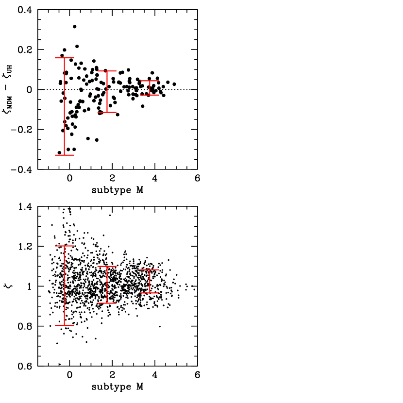
Figure 15.— The $\zeta$ parameter as a function of spectral subtype. Top: difference in $\zeta$ for the same stars measured at the two observatories (MDM and UH). The scatter provides an estimate of the measurement error on $\zeta$, which is significantly larger at earlier subtypes. Bottom: adopted values of $\zeta$ for all the stars in the survey. The larger scatter at subtypes M2 and earlier can be fully accounted by the measurement errors. The scatter at subtypes M3 and later is larger than the measurement error, and is thus probably intrinsic and is evidence for intrinsic metallicity scatter in the solar neighborhood.

6.1. Recalibration of the $\zeta$ parameter

The $\zeta_{TiO/CaH}$ parameter (denoted $\zeta$ for short) is a combination of the TiO5, CaH2, and CaH3 spectral indices which was shown to be correlated with metallicity in metal-poor M subdwarfs (Woolf, Lepine, & Wallerstein, 2009). The index was first described in Lépine, Rich, & Shara (2007), and a revised calibration has recently been proposed by Dhital et al. (2012). The index measures the relative strength of the TiO molecular band around 7,000Å with respect to the nearby CaH molecular band. In cool stars, in fact, the ratio between TiO and CaH is a function of both gravity and metallicity. The CaH band is noticeably stronger in giants (Mann et al., 2012), and this effect can be used as affective means to separate out M giants from M dwarfs using optical spectroscopy. In the higher gravity M dwarfs/subwarfs however, the TiO to CaH ratio is however believed to be mostly affected by metallicity, although young stars may show gravity effects as well.

The $\zeta$ parameter was originally introduced to rank metal-poor, main-sequence M stars into three metallicity classes (Lépine, Rich, & Shara, 2007); stars with $0.5<\zeta<0.825$ are formally classified as subdwarfs (sdM), $0.2<\zeta<0.5$ defines extreme subdwarfs (esdM), while a $\zeta<0.2$ identifies the star as an ultrasubdwarf (usdM). However, it is conjectured that $\zeta$ could be used to measure metallicity differences in disk M dwarfs, i.e. at the metal-rich end. Disk M dwarfs are generally found to have $0.9<\zeta<1.1$, though it is unclear if variations in $\zeta$ correlate with metallicity for values within that range. Measurement of Fe lines in a subset of M dwarfs and subdwarfs does confirm that the $\zeta$ parameter is correlated with metallicity (Woolf, Lepine, & Wallerstein, 2009), with $\zeta\simeq 1.05$ presumably corresponding to solar abundances. However there is a significant scatter in the relationship which raises doubts about the accuracy of $\zeta$ as a metallicity diagnostic tool.

A important caveat is that the TiO/CaH ratio is not sensitive to the classical iron-to-hydrogen ratio Fe/H, but rather depends on the relative abundance of $\alpha$-elements to hydrogen ($\alpha$/H) because O, Ca, and Ti are all $\alpha$-elements. Variations in $\alpha$/Fe would thus weaken the correlation between $\zeta$ and Fe/H. The $\alpha$/Fe abundance ratio is however relatively small in metal-rich stars of the thin disk ($\pm$0.05dex) disk stars, and are found to be significant ($\pm$0.2dex) mostly in more metal-poor stars associated with the thick disk and halo (Navarro et al., 2011). It is thus unclear whether typical $\alpha$/Fe variations would affect the $\zeta$ parameter significantly in our subset, which is dominated by relatively metal-rich stars.

On the other hand, it is clear that the index has significantly more leverage at later subtypes. This is because the strengths of both the TiO and CaH bands are generally greater, and their ratio can thus be measured with higher accuracy. The index is much leass reliable at earlier M subtypes however, and is notably inefficient for late-K stars.

A more important issue is the specific calibration adopted for the $\zeta$ parameter, which is a complicated function of the TiO5, CaH2, and CaH3 indices. The $\zeta$ parameter itself is defined as:

$$\zeta=\frac{1-{\rm TiO5}}{1-[{\rm TiO5}]_{Z_{\odot}}},$$ (14)

which in turns depend on $[{\rm TiO5}]_{Z_{\odot}}$, itself a function of CaH2+CaH3. The function $[{\rm TiO5}]_{Z_{\odot}}$ represents the expected value of the TiO5 index in stars of solar metallicity, for a given value of CaH2+CaH3. In (Lépine, Rich, & Shara, 2007), ${\rm TiO5}]_{Z_{\odot}}$ was defined as:

$$[{\rm TiO5}]_{Z_{\odot}}=-0.050-0.118\ {\rm CaH}+0.670\ {\rm CaH}^{2}$$

$$-0.164\ {\rm CaH}^{3}$$ (15)

where ${\rm CaH}={\rm CaH2}+{\rm CaH3}$. The more recent calibration of Dhital et al. (2012), on the other hand, uses:

$$[{\rm TiO5}]_{Z_{\odot}}=-0.047-0.127\ {\rm CaH}+0.694\ {\rm CaH}^{2}$$

$$-0.183\ {\rm CaH}^{3}-0.005\ {\rm CaH}^{4}.$$ (16)

The difference between the two calibrations is mainly in the treatment of late-K and early-type M dwarfs, as illustrated in Figure 14. When overlaid on the distribution of CaH2+CaH3 and TiO5 values from our current survey, however, the two calibrations fail to properly fit the distribution of data points at the earliest subtypes (high values of CaH2+CaH3 and TiO5). This results in the Lépine, Rich, & Shara (2007) overestimating the metallicity at earlier subtypes, while the Dhital et al. (2012) calibration tends to underestimate metallicity.

In any case, the evidence presented in §3.3 and §3.4 which shows that differences in spectral resolution and flux calibration can yield differences in the TiO5, CaH2, and CaH3 spectral indices of the same stars, also suggests that a calibration of the $\zeta$ parameter may only be valid for data from a particular observatory/instrument. A general calibration of $\zeta$ may only be adopted after corrections have been applied as described in Section 3.2. Because we do not have any star in common with the Dhital et al. (2012) subsample, we cannot verify the consistency of their $\zeta$ calibration to our data at this time. In addition, because we have now applied a correction to our MDM spectral index measurements, the Lépine, Rich, & Shara (2007) calibration of $\zeta$ may now be off, and should not be used for our sample.

Instead, we recalibrate the $\zeta$ parameter again, using our corrected spectral index values. Our fit of $\left[\rm TiO5\right]_{c}$ as a function of $\left[{\rm CaH}\right]_{c}=\left[{\rm CaH2}\right]_{c}+\left[{\rm CaH3}\right]_{c}$ yields:

$$[{\rm TiO5}]_{Z_{\odot}}=0.622-1.906\ (\left[{\rm CaH}\right]_{c})-2.211\ (\left[{\rm CaH}\right]_{c})^{2}$$

$$-0.588\ (\left[{\rm CaH}\right]_{c})^{3}.$$ (17)

We calculate the new $\zeta$ values using the corrected values of the TiO5 index, i.e.:

$$\zeta=\frac{1-{\rm\left[TiO5\right]_{c}}}{1-[{\rm TiO5}]_{Z_{\odot}}}.$$ (18)

All our values of $\zeta$ are listed in Table 3.

In order to evaluate the accuracy of the $\zeta$ measurements, we compared the values of $\zeta$ independently measured at both MDM and UH for the 146 stars in our inter-observatory subset. Values are compared in Figure 15 (top panel) which shows $\Delta\zeta=\zeta_{MDM}-\zeta_{UH}$ as a function of spectral subtype. We find a mean offset $\bar{\Delta\zeta}=-0.01$ and a dispersion $\sigma_{\Delta\zeta}=0.10$. The small offset indicates that the $\zeta$ measurements are generally consistent between the two observatories. The dispersion $\sigma_{\Delta\zeta}$, on the other hand, provides an estimate of the measurement accuracy. Splitting the stars in three groups, we find the mean offsets and dispersions $(\bar{\Delta\zeta},\sigma_{\Delta\zeta})$ to be (-0.086,0.244) for subtypes K7.0-M0.5, (-0.011,0.103) for subtypes M1.0-M2.5, and (0.008,0.036) for subtypes M3.0-M5.5. Assuming that stars do not show significant variability in those bands, we adopt the dispersions as estimates of the measurement errors on $\zeta$ for that particular subtype range. It is clear from Figure 14 that early type stars should have larger uncertainties in $\zeta$ because of the convergence of the iso-$\zeta$ lines. The best leverage for estimating metallicities from the TiO and CaH bandheads is at later types when the molecular bands and well developed.

The overall distribution of $\zeta$ values as a function of spectral subtype also shows a decrease in the dispersion as a function of spectral type (Figure 15, bottom panel). In early-type dwarfs (K7.0-M0.5), the scatter in the $\zeta$ values is relatively large, with $\sigma_{\zeta}\simeq 0.174$. It then drops to $\sigma_{\zeta}\simeq 0.100$ for subtypes M1.0-M2.5, and to $\sigma_{\zeta}\simeq 0.059$ for subtypes M3.0-M5.5. Note that the scatter in the M3.0-M5.5 bin is a factor 2 larger than the estimated accuracy of the $\zeta$ for that range, as estimated above. We suggests this to be evidence of an intrinsic scatter in the $\zeta$ values for the stars in our sample, which we allege to be the signature of a metallicity scatter. If we subtract in quadrature the $0.035$ measurement error on $\zeta$, we estimate the instrinsic scatter to be $\approx$0.05 units in $\zeta$. This intrinsic scatter, which presumably affects all subtypes equally, is unfortunately drowned in the measurement error at earlier subtypes ($<$M3).

6.2. Comparison with other metallicity diagnostics

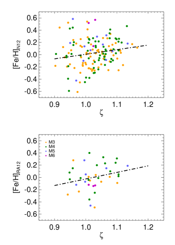
Figure 16.— Comparison between the $\zeta$ parameter values and independent metallicity measurements for subsets of M dwarfs in our survey. Top panel compares our $\zeta$ to the Fe/H estimated from the (V-K,M_K) calibration of Neves et al. (2012) for the same stars. Bottom panel compares our $\zeta$ values to the Fe/H estimated from the infrared K-band index by Rojas-Ayala et al. (2012). Both distribution show weak positive correlations.

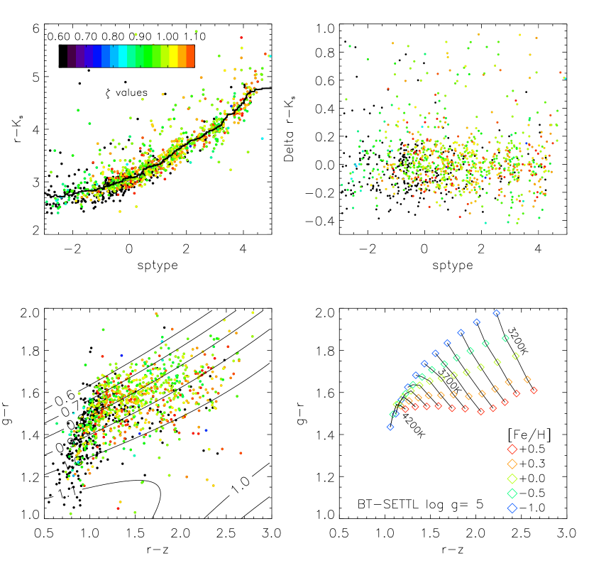
Figure 17.— SDSS photometry of M dwarf stars synthesized from SNIFS spectra and transmission functions convolved with unit airmass. Upper left: r-Ks (where Ks is from the 2MASS point source catalog) against M spectral subtype (where K7=-1 and K5=-2). Points are colored by the $\zeta$ parameter, which measures TiO/CaH ratio and is a metallicity diagnostic in the optical. The $\zeta$ values are undefined for late K stars, which are plotted as black points. The black curve is a running median (N=81). Upper right: difference of r-Ks with respect to the running median vs. spectral type, showing no obvious correlation with zeta. Lower left: g-r vs. r-z, showing an apparent correlation between these colors and $\zeta$. The contours are the empirical function for $\zeta$ derived by West et al. (2011). Lower right: SDSS g-r vs. r-z colors generated by the PHOENIX/BT-SETTL model (Allard, Hauschildt, & Schweitzer, 2000) for log g=5, Teff=3500K-4200K, and five different values of the metallicity as noted in the legend. The model predicts the more metal-rich M dwarfs to have bluer g-r colors, while being redder in r-z. The color dependence on metallicity in most pronounced in late-type stars, and nearly vanishes at K7/M0.

To test our $\zeta$ as a tracer of metallicity for dM stars from M3 to M6, we compared the values to two recent [Fe/H] calibration techniques for M dwarfs with solar metallicities. First, we used the photometric calibration of Neves et al. (2012), which is based on optical-to-infrared V-K color and absolute magnitude M_K. The method is sensitive to small variations in V-K/M_K and thus requires an accurate, geometric parallax. A total of 143 stars in our sample have parallaxes, and thus can have their metallicities estimated with the method. Figure 16 (top panel) plots the estimated $\rm[Fe/H]$ as a function of $\zeta$ for those 143 stars. The distribution shows significant scatter, but we find a weak correlation of $\rm[Fe/H]$ with $\zeta$, which we fit with the relationship:

$$[Fe/H]_{\rm N12}=0.750\zeta-0.743.$$ (19)

Stars are scattered about this relationship with a 1-$\sigma$ dispersion of 0.383 dex. One drawback of the photometric metallicity determination is that it assumes the star to be single. Unresolved double stars appear overluminous at a given color, and will thus be determined to be metal-rich. Also, young and active stars often appear overluminous in the color-magnitude diagram (Hawley et al., 2002), and their metalicities based on V-K/M_K would also be overestimated. Multiplicity and activity could therefore contribute in the observed scatter. Stars with $[Fe/H]_{\rm N12}>0.4$, in particular, could be overluminous in the V-K/M_K diagram, as their $\zeta$ does not suggest them to be metal-rich.

Next, we retrieve metallicity measurements from Rojas-Ayala et al. (2012), who estimated $[Fe/H]$ based on the spectroscopic calibration from infrared K-band atomic features. Their list has 37 stars in common with our survey. The $[Fe/H]$ values are plotted as a function of our $\zeta$ values in the bottom panel of Figure 16. Again there is significant scatter, but we also find a weak correlation which we fit with the relationship:

$$[Fe/H]_{\rm RA12}=1.071\zeta-1.096,$$ (20)

about which there is a dispersion of 0.654 dex. The statistics are relativey poor at this time, and more metallicity measurements in the infrared bands would be useful.

The weak correlation found in both distribution is interesting in itself. Using a sample of stars spanning a wide range of metallicities and $\zeta$ values, including metal-poor M subdwarfs, extreme subdwarfs (esdM), and extremely metal-poor ultrasubdwarfs (usdM), Woolf, Lepine, & Wallerstein (2009) determined a relationship of the form $[Fe/H]=-1.685+1.632\zeta$, over the range $0.05<\zeta<1.10$. All the stars in the two distributions from the present survey have $\zeta$ values between $\sim$0.9 and $\sim$1.2, and thus represent the metal-rich end of the distribution. The weaker slopes we find in our correlations (0.75 and 1.07) may indicate that the relationship levels off at high metallicity end, which would make $\zeta$ much less useful as a metallicity diagnostic tool in Solar-metallicity and metal-rich M dwarfs. The correlations are however weak, and more accurate measurement of $\zeta$ and $Fe/H$ would be needed to verify this conjecture.

6.3. The one M subdwarf: PM I20050+5426 (V1513 Cyg)

The primary purpose of the $\zeta$ parameter is the identification of metal-poor M subdwarfs, for which it has already proven effective. By definition, M subdwarfs are stars with $\zeta<$0.82 (Lépine, Rich, & Shara, 2007). Though we have a few stars with values of $\zeta$ just marginally under 0.82, only one star clearly stands out as a definite M subdwarf: the star PM I20050+5426 (= Gl 781) which boasts a $\zeta=0.58$ well within the M subdwarf regime. The star also clearly stands out in Figure 14 where it lies noticeably below the main locus at TiO5${}_{c}\simeq$0.75.

PM I20050+5426 is also known as V1513 Cyg, a star previously identified as an M subdwarf by Gizis (1997), and one clearly associated with the Galactic halo (Fuchs & Jahreiss, 1998). The star is also notorious for being a flare star, with chromospheric activity due not to young age but to the presence of a low-mass companion on a close orbit (Gizis, 1998). Our own spectrum indeed shows a relatively strong line of H$\alpha$ in emission, which is extremely unusual for an M subdwarf. It is an interesting coincidence that the brightest M subdwarf in the northern sky should turn out to be a peculiar object.

In any case, because the TiO molecular bands are weaker in M subdwarfs than they are in M dwarfs, the use of TiO spectral indices for spectral classification leads to underestimates of their spectral subtype. The convention for M subdwarfs is rather to base the classification on the strengths of the CaH bandheads (Gizis, 1997; Lépine, Rich, & Shara, 2003, 2007). We adopt the same convention here, and recalculate the subtype from the mean of Equations 6 and 7 only (CaH2 and CaH3 indices). We thus classify PM I20050+5426 as an sdM2.0, which is one half-subtype later than the sdM1.5 classification suggested by (Gizis, 1997).

6.4. Photometric dependence on metallicity

A prediction of current atmospheric models is that metallicity variations in M dwarfs yield significant variations in optical broadband colors (Allard et al., 2000). The metal-poor M subdwarfs have in fact long been known to have bluer V-I colors than the more metal-rich field M dwarfs of the same luminosity (Monet et al., 1992; Lépine, Rich, & Shara, 2003). The bluer colors are due to reduced TiO opacities in the optical, which make the spectral energy distribution of M subdwarfs closer to that of a blackbody, while it makes the metal-rich M dwarfs display extreme red colors.

Interestingly, the SDSS $g-r$ color index shows the opposite trend, and is bluer in the more metal-poor stars. This is because the TiO bands very strongly depress the flux in the 6000Å-7000Å (r-band) range, an effect which in fact makes the metal-rich M dwarfs degenerate in $g-r$, as the increased TiO opacities in cooler stars balance out the reduced flux in $g$ from lower T_eff. This effect is much weaker in metal-poor stars due to the reduced TiO opacity, which makes metal-poor stars go redder as they are cooler, as one would normally expect. This has been observed in late-type M subdwarfs, which have significantly redder color that field M dwarfs (Lepine & Scholz, 2008). The color dependence of M dwarfs/subdwarfs on metallicity is also predicted by atmospheric models. Figure 17 (bottom-right panel) shows the predicted $g-r$ and $r-z$ colors from the PHOENIX/BT-SETTL model of Allard, Hauschildt, & Schweitzer (2000). The models corroborate observations and predict redder $g-r$ colors in metal-poor stars.

Although $ugriz$ photometry is not available for our stars (all of them are too bright and saturated in the Sloan Digital Sky Survey), it is possible to use the well-calibrated SNIFS spectrophotometry to calculate synthetic broadband $riz$ magnitudes for the subset of stars observed at UH. We first examine any possible correlation between the optical to infrared $r-K_{S}$ color (taken as a proxy for V-I) and the $\zeta$ index. Figure 17 plots $r-K_{s}$ as a function of spectral subtype, with the dots color-coded for the $\zeta$ values of their associated M dwarf (top-left panel). We find a tight relationship between $r-K_{s}$ and spectral subtype, which we fit using a running median. The residuals are plotted in the top-right panel, and show no evidence of a correlation with $\zeta$. There are a significant number of outliers with redder $r-K_{s}$ colors than the bulk of the M dwarfs: these likely indicate systematic errors in estimating the synthetic $r$ band magnitudes. The absence of any clear correlation suggests that an optical-to-infrared color such as $r-K_{S}$ is not sensitive enough to detect small metallicity variations, at least at the metal-rich end.

The synthetic $g-r$ and $r-z$ colors are plotted in Figure 17 (lower-left panel). The redder stars ($r-z$¿1.2) show a wide scatter in $g-r$, on the order of what is predicted for stars with a range of metallicities $-0.5<[Fe/H]<0.5$. Though we do not find a clear trend between the synthetic $g-r$ colors and the $\zeta$ values measured in the same stars, the high-$\zeta$ stars (red and orange dots on the plot) do seem to have lower values of $g-r$ on average than the low-$\zeta$ ones (green dots). The trend is suggestive of a metallicity link to both the $g-r$ colors and the $\zeta$ values, and should be investigated further with data of higher precision.

7. Chromospheric activity

Table 7Survey stars: distances, kinematics, and activity.

Star name	$\pi_{trig}$	$\pi_{phot}$	$\pi_{spec}$	U	V	W	EWHA	H$\alpha$	Xray	UV
	$\arcsec$	$\arcsec$	$\arcsec$	km s-1	km s-1	km s-1	Å	active	active	active
PM I00006+1829	$\cdots$	$\cdots$	$\cdots$	$\cdots$	$\cdots$	$\cdots$	$\cdots$	-	-	-
PM I00012+1358S	$\cdots$	0.030$\pm$ 0.008	0.028$\pm$ 0.008	-13.9	12.1	$\cdots$	0.41	-	-	-
PM I00033+0441	0.0342$\pm$ 0.0032	0.031$\pm$ 0.008	0.030$\pm$ 0.009	8.5	-6.8	$\cdots$	0.39	-	-	-
PM I00051+4547	0.0889$\pm$ 0.0014	0.078$\pm$ 0.021	0.083$\pm$ 0.024	-38.2	$\cdots$	-15.9	0.47	-	-	-
PM I00051+7406	$\cdots$	$\cdots$	$\cdots$	$\cdots$	$\cdots$	$\cdots$	$\cdots$	-	-	-
PM I00077+6022	$\cdots$	0.078$\pm$ 0.031	0.091$\pm$ 0.027	-15.1	$\cdots$	-4.4	-3.11	Y	-	-
PM I00078+6736	$\cdots$	0.046$\pm$ 0.012	0.055$\pm$ 0.016	5.1	$\cdots$	-8.5	0.39	-	-	-
PM I00081+4757	$\cdots$	0.071$\pm$ 0.028	0.061$\pm$ 0.018	7.9	$\cdots$	1.8	-2.93	Y	-	Y
PM I00084+1725	0.0460$\pm$ 0.0019	0.040$\pm$ 0.011	0.040$\pm$ 0.012	11.2	0.7	$\cdots$	0.41	-	-	-
PM I00088+2050	$\cdots$	0.078$\pm$ 0.031	0.080$\pm$ 0.024	9.5	$\cdots$	-10.1	-4.64	Y	-	Y
PM I00110+0512	0.0233$\pm$ 0.0038	0.032$\pm$ 0.009	0.031$\pm$ 0.009	-48.5	-14.3	$\cdots$	0.35	-	-	-
PM I00113+5837	$\cdots$	$\cdots$	$\cdots$	$\cdots$	$\cdots$	$\cdots$	$\cdots$	-	-	-
PM I00118+2259	$\cdots$	0.055$\pm$ 0.022	0.054$\pm$ 0.016	-3.0	$\cdots$	-16.7	0.30	-	Y	-
PM I00125+2142En	0.0358$\pm$ 0.0028	0.023$\pm$ 0.006	0.024$\pm$ 0.007	-5.9	$\cdots$	-32.5	0.44	-	-	-
PM I00131+7023	$\cdots$	0.037$\pm$ 0.010	0.037$\pm$ 0.011	-6.2	$\cdots$	16.8	0.37	-	-	-

Figure 18.— Fraction of active stars as a function of the spectral subtype M. The rise at later subtypes is consistent with earlier studies of field M dwarf, which shows increased activity levels in mid-type M dwarfs. The fraction level at later subtype is however higher than that measured in the SDSS spectroscopic catalog.

To evaluate the presence of H$\alpha$ in emission in our M dwarfs, we used the H$\alpha$ equivalent width index EWHA defined as:

$$EWHA=100{\rm\AA}\left[1-\frac{14{\rm\AA}\int_{6557.61}^{6571.61}S(\lambda)d\lambda}{100{\rm\AA}\left(\int_{6500}^{6550}S(\lambda)d\lambda+\int_{6575}^{6625}S(\lambda)d\lambda\right)}\right],$$ (21)

where $S(\lambda)$ is the observed spectrum. The EWHA index measures the flux in a region (6557.61Å-6571.61Å), which includes the $H\alpha$ line, in relation to a pseudo-continuum region spanning 6500Å-6550Å and 6575Å-6625Å; the calculation provides a value in units of wavelength (Å) like the traditional equivalent width. Note that for an $H\alpha$ line in emission, values of the EWHA index are negative, following convention. Assuming the W1-W2 region to measure the true spectral continuum, then the EWHA index would measure the true equivalent width of $H\alpha$. As it turns out, the $W1-W2$ region often has a higher mean flux than the $W3-W4$ region without the $H\alpha$ emission component, which means that the EWHA index systematically underestimate the equivalent width of the $H\alpha$ line. The index is however reproducible and more convenient for automated measurement than, e.g. manual evaluation of the equivalent using interactive software such as IRAF.

The EWHA index was measured for all spectra in our sample, and used to flag active stars. Following West et al. (2011), we defined a star to be chromospherically “active” if EWHA $<-0.75\AA$, which usually corresponds to a clearly detectable $H\alpha$ line in emission. Values of the EWHA index are listed in Table 7. Under the above criterion, 171 M dwarfs in our survey are considered active.

Hawley, Gizis, & Reid (1996) found that active stars (by their criterion, EW(H$\alpha$) $>1\AA$) have slightly redder $V-K$ colors for the same value of TiO5 index, an effective temperature proxy. We calculated a median ($N=30$) locus of $V-K$ vs. TiO5 index for our entire sample and found that 13 active stars are bluer than this locus, while 45 are redder, seemingly confirming their result. The large scatter in $V-K$ colors however prevents us from quantifying this offset more precisely.

The fraction of stars that are active at each spectral subtype is shown in Figure 18, with error bars computed from the binomial distribution. The increase in the active fraction with spectral type is consistent with previous studies (Joy & Abt, 1974; Hawley, Gizis, & Reid, 1996; West et al., 2004, 2008; Kruse et al., 2010; West et al., 2011). Our active fractions are higher at subtype M4-M6 than the Hawley, Gizis, & Reid (1996) results, even when using their criterion to define active stars (see above). This may be a result of a slightly different definition for EW, or a result of the relatively small number of objects. Our active fractions are also higher than the West et al. (2011) results at each subtype. This discrepancy is likely caused by the magnitude limit imposed in our survey: our objects are all nearby, and relatively close to the Galactic plane (see Section 8), which makes them statistically younger, as also suggested West et al. (2011). The active fractions for our stars are closer to the active fractions for the West et al. (2011) stars in bins of stars closest to the Galactic plane.

Another chromospheric activity diagnostic in M dwarfs is the detection of X-rays. M dwarfs that are X-ray bright are often young, and this has been used to identify members of nearby young moving groups (e.g., Gaidos, 1998; Zuckerman et al., 2001; Torres et al., 2006), and other young stars in the Solar Neighborhood (Riaz, Gizis, & Harvin, 2005). Most recently, Shkolnik et al. (2009, 2012) and Schlieder et al. (2012) have used the ratio of ROSAT X-ray flux to 2MASS J or K-band flux to identify candidate members of young moving groups. This technique is particularly effective for objects $\lesssim 70$pc away, which includes all the stars in our sample. The Lépine & Gaidos (2011) catalog, from which our targets are drawn, was already cross-matched to the ROSAT All-Sky Bright Source Catalog (Voges et al., 1999) and the ROSAT All-Sky Survey Faint Source Catalog (Voges et al., 2000).

We have computed the X-ray flux for our survey stars from the measured count rate and hardness ratio (HR1) using the prescription in Schmitt, Fleming, & Giampapa (1995). Figure 19 shows the distribution of X-ray flux as a function of $V-K$ color, for the 290 M dwarfs with ROSAT detections. Dots are color-coded according to the strength of the H$\alpha$ emission, as measured by the EWHA index. As expected, M dwarfs with strong H$\alpha$ emission also tend to be more X-ray bright. Objects with $\log F_{X}\ F_{K}>-2.6$ (above the dashed line in Figure 19) are considered bright enough in X-ray to qualify as chromospherically active, following the definition of Schlieder et al. (2012). Some 154 of the X-ray sources are active based on their EWHA values, and all of them also qualify as active stars based on their X-ray fluxes. On the other hand, 53 M dwarfs identified as active based on X-ray flux do not display significant H$\alpha$ emission in our spectra; most of them tend to be earlier M dwarfs, in which H$\alpha$ emission is not as easily detected as in later type objects because of their higher continuum flux near $\lambda 6563\AA$. There are also 22 stars in our survey which are active based on $H\alpha$ but are not detected by ROSAT. This suggests that only two thirds of the “active” stars will be diagnosed as such from both X-ray and H$\alpha$ emission, while the other third will show only either. This could be due to source confusion in the ROSAT X-ray survey, variability in either X-ray or H$\alpha$ emission, or, in the case of the X-ray flux, non-uniform sky coverage by ROSAT. We calculated the luminosity ratio index $L_{X}/L_{H\alpha}$ of active stars, as defined by the criterion EW(H$\alpha$) $>1\AA$ following the procedure of Hawley, Gizis, & Reid (1996), and adopting the relation $V-R\approx 0.7+0.06{\rm SpTy}$ to estimate an $R$ magnitude and the continuum flux at the H$\alpha$ line. We find that the ratio is insensitive to bolometric magnitude and spectral type, and has a median value of 0.85. This is higher than the Hawley, Gizis, & Reid (1996) average of $\sim 0.5$, and may in part be due to Malmquist bias in the flux-limited ROSAT survey favoring the inclusion of the most X-ray luminous stars, as well as greater variation in the ratio because of the elapsed time (two decades) between the ROSAT survey and our observations.

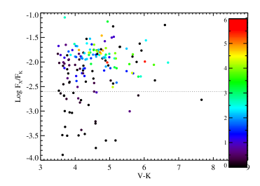
Figure 19.— X-ray luminosity normalized by the flux in the infrared K_s band, plotted as a function of the optical-to-infrared color $V-K$, for stars in our sample which have counterparts in the ROSAT all-sky points source catalog. The color scheme shows the H$\alpha$ equivalent width; active stars are found to have large X-ray flux, as expected from chromospheric activity.

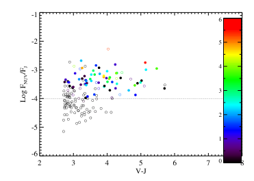
Figure 20.— Normalized near-UV flux as a function of the optical-to-infrared $V-K_{s}$ color. The color scheme shows the strength of the H$\alpha$ equivalent width. Closed circles show stars identified as active based on X-ray emission, closed circles show stars with low or no detection in ROSAT.

Active stars can also be identified from ultra-violet excess, as suggested in Section 3.4. Shkolnik et al. (2011, 2012) showed that GALEX UV fluxes can identify young M dwarfs in nearby moving groups, and can identify active stars to larger distances. Figure 20 shows the GALEX NUV to 2MASS J flux ratio, for the objects with UV detections. The dashed line shows the selection criteria of Shkolnik et al. (2011). Dot colors represent the EWHA index values for the stars, while filled circles indicate objects with $\log F_{X}/F_{K}>-2.6$, i.e. stars whose X-ray flux does not identify them as being active. Overall, there is a good correpondence between the different activity diagnostics. However, there are some stars identified as active based on UV flux that are not identified as such from their X-ray and/or $H\alpha$ emission. Again this suggests that a complete identification of active M dwarfs in the solar vicinity may require a combination of diagnostic features.

In any case our survey, which combines X-ray, UV, and $H\alpha$ diagnostics, provides a valuable subset for identifying low-mass young stars in the Solar Neighborhood, and may potentially yield new members of young moving groups, or even the identification of new moving groups. The last three columns in Table 7 display flags for stars found to be active from either H$\alpha$, X-ray, or UV flux. The flag indicates activity by a “Y”. Absence of a flag does not necessarily indicate absence of activity: the GALEX survey does not cover the entire sky, and the ROSAT X-ray survey is not uniform in sensitivity, so a non-detection in either does not necessarily indicate quiescence. Activity diagnostics could also be time-variable. H$\alpha$ equivalent width is particular are know to be variable on various timescales (Bell et al., 2012). In any case, there is a good correlation between the different diagnostics. We flag 175 stars as active based on H$\alpha$, 42 based on X-ray emission, and 172 based on UV excess. Overall, 252 stars are assigned one or more activity flags: 19 stars have all three flags on, 99 stars get two flags, and 137 get only one.

8. Distances and kinematics

8.1. Spectroscopic distances

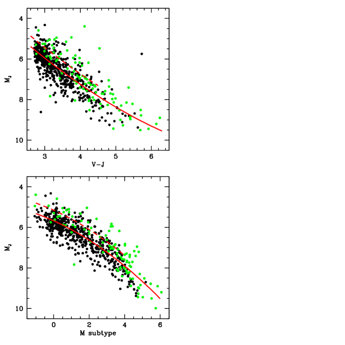
Figure 21.— Absolute visual ($M_{V}$) and infrared ($M_{J}$) magnitudes for the 631 stars in our survey for which geometric parallax measurements exist in the literature. Top panels: absolute magnitudes against $V-J$ color, which follow the color-magnitude relationship used in Lépine & Gaidos (2011) to estimate photometric distances. Bottom panel: absolute magnitudes as a function of spectral subtype, based on the spectral-index classification described in this paper. Active stars are plotted in green, and are found to be overluminous at a given $V-J$ color and given spectral subtype, compared with non-active stars. The offset in notable for stars of earlier M subtypes (or bluer $V-J$ colors).

Astrometric parallaxes are available for 631 of the stars in our sample, spanning the full range of colors and spectral subtypes. We combine these data with our spectroscopic measurements to re-evaluate photometric and spectroscopic distances calibrations for M dwarfs in our census. Absolute visual magnitudes $M_{V}$ are calculated and are plotted against both $V-J$ color and spectral subtype in Figure 21. M dwarfs with signs of activity (H$\alpha$, UV, X-ray) are plotted in green, other stars are plotted in black. The solid red lines are the best-fit second order polynomials, when both active and inactive stars are used, and after elimination of 3$\sigma$ outliers. The equations for the fits, where $spT$ is the spectral type (K7 is -1 and M0=0, etc) are:

$$M_{J}=1.194+1.823(V-J)-0.079(V-J)^{2}$$ (22)

$$M_{J}=5.680+0.393(SpT)+0.040(SpT)^{2}$$ (23)

where SpT are the spectral types, and with the least-squares fit performed after exclusion of 3-sigma outliers. The 1$\sigma$ dispersion about these relationships are $\pm 0.61$ mag for (M_J,V-J), and $\pm 0.52$ mag for (M_J,SpT). The smaller scatter in the spectroscopic relationship suggests that spectroscopic distances may be marginally more accurate than the photometric ones. We suspect that the larger uncertainty on the photographic $V$ magnitudes may be the cause.

The most notable feature in the diagrams is that active stars appear to be systematically more luminous than non-active stars. This corroborates the observation made previously by Hawley et al. (2002), as part of the PMSU survey. Hawley et al. (2002) found that active stars were more luminous by 0.48mag in a diagram of $M_{K}$ against TiO5 index, used as proxy for spectral subtype. For stars in our census, we find that among stars of spectral subtype M2 and earlier, active stars are on average 0.46mag more luminous at a given subtype than non-active stars; in the color-magnitude diagram, bluer stars of colors $V-J<4.0$ which are active are on average 0.47mag more luminous than non-active stars of the same color. Both values agree well with the values quoted by Hawley et al. (2002). The systematic overluminosity of active stars is also responsible for some of the scatter in the color-magnitude and spectral-type magnitude relationships. If we exclude active stars, the scatter about the color-magnitude relationship fals marginally to $\pm 0.58$, and the scatter in the spectral-type magnitude relationship falls to $\pm 0.49$.

The offset in absolute magnitude between active and non-active stars suggests that spectroscopic and photometric distances would be more accurate for active stars in our census if their estimated absolute magnitudes were made 0.46mag brighter that suggested by Equation 23. We therefore adopt the following relationships to be applied only on active stars of subtype M2.5 and earlier:

$${[M_{J}]}_{early-active}=0.734+1.823(V-J)-0.079(V-J)^{2}$$ (24)

$${[M_{J}]}_{early-active}=5.220+0.393(SpT)+0.040(SpT)^{2}$$ (25)

Again we define as “active” any star which qualifies as such base on any one of our criteria (H$\alpha$, UV, X-ray). There are several reasons that would explain why active, early-type stars are more luminous at a given subtype. Activity in an early-type M dwarf could mean that the star is younger (Delfosse et al., 1998); early-type M dwarfs with ages $<100$Myr are known to be overluminous at a given color, due to lower surface gravity (Shkolnik et al., 2012). Older stars could remain active due to interaction with a close companion (Morgan et al., 2012), in which case the active stars would also appear overluminous due to this unresolved companion. Late-type M dwarfs, however, can remain active for long periods of time, and would thus not require the star to be young or have a close companion.

Splitting the active and inactive stars results in lowering the scatter of non-active stars in the subtype-magnitude relationship (to $\pm$0.5mag). Overall, our spectroscopic distances for non-active M dwarfs provide a $1\sigma$ uncertainty of $\pm 26\%$ on the distance. For active stars, we find a scatter of $\pm$0.6mag, which suggests distance uncertainties of $\pm 32\%$. Our photometric distances estimated from (V,V-J) have similar though perhaps slightly larger uncertainties. Photometric and spectroscopic parallaxes, estimated from the above relationships for active and non-active stars, are listed in Table 7.

We estimated the effect of two relevant sampling biases on the calibration between $M_{J}$ and $V-J$ color. In Eddington bias, photometric errors scatter more numerous, bluer, and intrinsically brighter stars to redder apparent colors than redder stars are scattered to bluer apparent colors (Eddington, 1913). The net effect is to make stars at a given apparent color appear more luminous than they are. In Lutz-Kelker (LK) bias, a form of Malmquist bias, errors in trigonometric prallax will scatter more numerous and more distant stars with lower parallax to higher apparent parallax values, making them appear less luminous than they are (Lutz & Kelker, 1973). By taking the derivative of $M_{J}$ with respect $V-J$ color, multiplying by the derivative of the number of stars in our $J$-magnitude-limited catalog with respect to $M_{J}$, assuming that the errors in $V-J$ are gaussian-distributed with standard deviation $\sigma_{V-J}$, and integrating over the distribution, we find the Eddington bias in $M_{J}$ to be;

$$\Delta_{E}=-\ln 10\left[1.918=0.178\left(V-J\right)\right]^{2}\left(0.6-0.4\gamma\right)\sigma_{V-J}^{2},$$ (26)

where $\gamma$ is the power-law index of a luminosity function for M stars which we take to be 0.325. Performing a similar derivation for the effect of L-K bias on $M_{J}$, we find:

$$\Delta_{LK}=\frac{15}{\ln 10}\sigma_{\pi}^{2},$$ (27)

where $\sigma_{\pi}$ is the fractional error in parallax. Using published parallax errors for our Hipparcos stars and adopting a conservative $\sigma_{V-J}=0.05$, we find that L-K bias usually dominates over Eddington bias and that 74% of our stars have a total bias of less than +0.2 magnitudes. A running median ($N=100$) vs. $V-J$ color is highest ($\sim 0.15$) for the bluest ($V-J=2.7$) stars and falling to less than +0.05 magnitudes for $V-J>3.3$. An analogous analysis can be performed for the bias in $M_{J}$ vs. spectral type, with a similar result. To debias values of $M_{J}$, these values should be subtracted from our calibration but we do not perform that operation here because of the small magnitude of the effect, which would overestimate distances by about 2% on average. The correction would also seem negligible compared with the intrinsic scatter in our color-magnitude and subtype-magnitude relationships are of order $\pm 0.5-0.6$, much larger than the L-K correction.

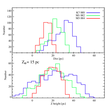
Figure 22.— Top: distribution of spectroscopic distances for the stars in our survey, shown for three ranges of spectral subtypes. Early-type stars are clearly sampled over a larger volume, which explains why they dominate our survey. Bottom: distribution of Galactic scales heights for the same stars, assuming that the Sun is hovering 15 pc sbove the Galactic midplane. As expected from our magnitude-limited sample, stars of later spectral subtypes (and lower luminosity) are found at shorter distances. Our survey samples a region well within the Galactic thin disk.

Figure 22 shows the distribution of photometric distances for our complete sample using Equation 23 and the M_J=M_J(V-J) color-magnitude relationship. The spectral subtypes are plotted in separate colors and demonstrates that the earlier-type stars, which are intrinsically brighter, are sampled to significantly larger distances compared with the later-type stars. In the 20pc volume, the M3-M4 stars still appear to dominate. We also plot the Galactic height of the stars in our sample, adopting a Galactic height of 15 pc for the Sun (Cohen, 1995; Ng et al., 1997; Binney, Gerhard, & Spergel, 1997). It is clear that our survey is largely contained within the Galactic thin disk, and barely extends south of the midplane. This is consistent with the relative absence of metal-poor stars associated with the thick disk and halo.

8.2. Kinematic analysis

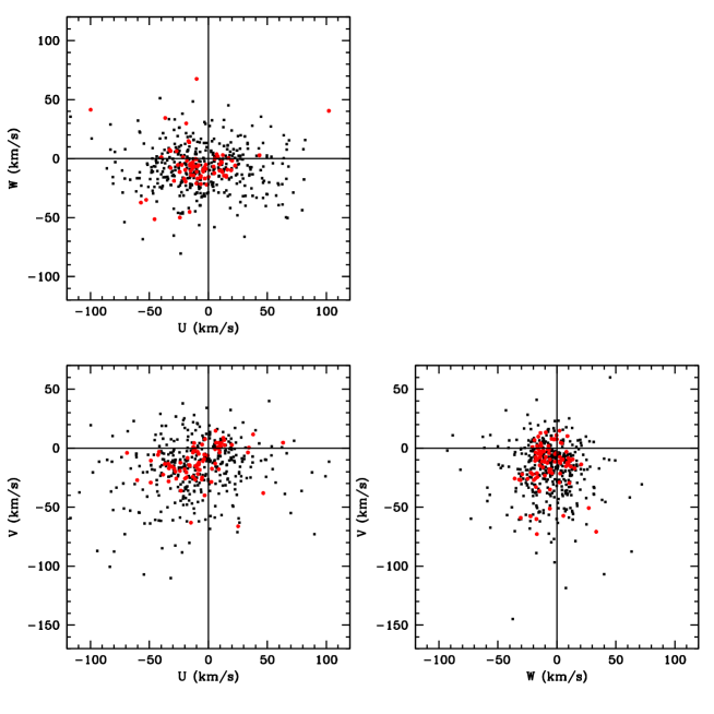
Figure 23.— Velocity-space projections for the M dwarfs in our survey. Velocies are calculated based on photometric distances and proper motions alone (no radial velocities used). Each star in our census is thus displayed in only one panel, which corresponds to the projection in which the radial velocity of the star has the smallest contribution. Stars with significant levels of H$\alpha$ emission, i.e. chromospherically active M dwarfs, are plotted in red.

Accurate radial velocities are not available for most of the stars in our sample, which prevents us from calculating the full (U,V,W) components of motion for each individual star. However, it is possible to use the distance measurements (for stars with parallaxes) or estimates (for stars with no parallax), and combine them to the proper motions to evaluate with some accuracy at least two of these components for each star. More specifically, we calculate the (U,V,W) components by assuming that the radial velocities $R_{V}=0$. We then consider the (X,Y,Z) positions of the stars in the Galactic reference frame, from the distances and sky coordinates. For stars with the largest component of position in +X or -X, the radial velocity mostly contibute to U, and has minimal influence on the values of V and W. Likewise stars with the largest component of position in +Y or -Y (+Z or -Z) make good tracers of the velocity distribution in U and W (U and V). We use this to assign any one of (U,V) or (U,W) or (V,W) velocity component doublet to every M dwarf in our catalog. Estimated values of the components of velocity are listed in Table 7. For each star, one of the components is missing, which is the component that would most depend on the radial velocity component based on the coordinates of the star. Again, the other two components are estimated only from proper motion and distance. For the distance, we use the trigonometric parallaxes whenever available; otherwise the spectroscopic distances as are used, based on the raltionships described in the previous section.

The resulting velocity distributions are displayed in Figure 23. We measure mean values of the velocity components using all allowable values and find:

$$<U>=-8.1~{}{\rm kms^{-1}},\sigma_{U}=32.8~{}{\rm kms^{-1}},$$

$$<V>=-17.0~{}{\rm kms^{-1}},\sigma_{V}=22.8~{}{\rm kms^{-1}},$$

$$<W>=-6.9~{}{\rm kms^{-1}},\sigma_{W}=19.3~{}{\rm kms^{-1}}.$$

The values are also largely consistent with those found from the PMSU survey and desribed in (Hawley, Gizis, & Reid, 1996). They are also remarkably similar to the moments of the velocity components calculated by Fuchs et al. (2009) for SDSS stars of the Galactic thin disk, and which are $<U>=-8.6,\sigma_{U}=32.4$, $<V>=-20.0,\sigma_{V}=23.0$, and $<W>=-7.1,\sigma_{W}=18.1$. The agreement suggests that our distance estimates are reasonably accurate, and it corroborates earlier results about the kinematics of the local M dwarf population which indicate a larger scatter of velocities in $U$. The mean values of $<U>$ and $<V>$ are consistent with the offsets from the local standard of rest as described in Dehnen & Binney (1998)

Active stars are found to have significantly smaller dispersions in velocity space. All 252 stars with at least one activity flags (i.e. stars found to be active either from H$\alpha$, X-ray flux, or UV excess) are plotted in red in Figure 23. Those active stars have first and second moments:

$$<U>=-9.3~{}{\rm kms^{-1}},\sigma_{U}=25.2~{}{\rm kms^{-1}},$$

$$<V>=-13.4~{}{\rm kms^{-1}},\sigma_{V}=16.8~{}{\rm kms^{-1}},$$

$$<W>=-6.6~{}{\rm kms^{-1}},\sigma_{W}=15.3~{}{\rm kms^{-1}}.$$

The values are consistent with (Hawley, Gizis, & Reid, 1996), who also reported that active M dwarfs tend to have a smaller scatter compared with inactive M dwarfs. The smaller dispersion values suggest that these active stars may be significantly younger than the average star in the Solar Neighborhood.

In any case, we also note that the velocioty space distribution is non-uniform and shows evidence for substructure. Our M dwarf data shows velocity-space substructure as that observed and described in Nordstrom et al. (2004); Holberg, Nordstrom, & Andersen (2008) for solar-type stars in the vicinity of the Sun. This substructure is sometimes referred to as “streams” or “moving groups”, although an analysis by Bovy & Hog (2010) shows that these groups do not represent coeval populations arising from star-formation episodes. The velocity-space substructure is more likely transient and associated with gravitational perturbations which are the signature of the Galactic spiral arms Quillen & Minchev (2005) and the Galactic bar Minchev et al. (2012). A simple description of the velocity-space distribution in terms of means values and dispersions, or as velocity ellipsoid, is therefore only a crude approximation of a more complex and structured distribution.

Finally, we note that the stars of our catalog that were previously part of the CNS3 and stars with measured trigonometric parallaxes (e.g. from the Hipparcos catalog) tend to have larger velocity dispersions, with $(\sigma_{U},\sigma_{V},\sigma_{W})$=(38.4,25.9,23.1), while the newer stars have $(\sigma_{U},\sigma_{V},\sigma_{W})$=(26.2,19.4,15.3). The difference could be due to systematic underestimation of the photometric/spectroscopic distances, but a more likely explanation is that the CNS3 and parallax subsample suffers from proper motion selection. This is because most of the CNS3 stars and M dwarfs monitored with Hipparcos were selected from historic catalogs of high proper motion stars, which have a higher limit than the SUPERBLINK proper motion catalog used in the LG2011 selection. This kinematic bias means that the current subset of M dwarfs monitored for exoplanet programs suffers from the same kinematic bias, which could possibly introduce age and metallicity selection effects.

9. Conclusions

We have now compiled spectroscopic data for a nearly complete list of M dwarfs in the northern sky with apparent magnitudes $J<9$. Our survey identifies a total of 1,403 very bright M dwarfs. Our new catalog provides spectral subtypes and activity measurements ($H\alpha$ emission) for all stars, as well as a rough indicator of metallicity in the guise of the $\zeta$ parameter, which measures the ratio of TiO to CaH bandstrengths. Only one of the stars in the survey is unambiguously identified as a metal-poor M subdwarf (PM I20050+5426 = V1513 Cyg).

Our target stars were identified from the all-sky catalog of bright M dwarfs presented in Lépine & Gaidos (2011). As such, our spectroscopic survey suffers from the same selection effects and completeness issues. The completeness and bias of the SUPERBLINK proper motion survey, from which these stars were selected is discussed a length in Lépine & Gaidos (2011). In the northern hemisphere, the SUPERBLINK catalog is complete for proper motions $\mu>40$ mas^-1. We show in §4 that there is a kinematic bias in the catalog which excludes stars with very low transverse motions (in the plane of the sky), but the low proper motion limit means that less than 5% of stars within 65 parsecs of the Sun are in fact excluded in the selection. In addition, we estimate that $\approx$5% of the nearby, bright M dwarfs may have escaped our target selection scheme due to faulty magnitudes. Therefore, we estimate that our census most likely include $>90\%$ of all existing M dwarfs in the northern sky with $J<9$. Early-type K7-M1 dwarfs have absolute magnitudes $M_{J}\approx 5.5$, and our $J<9$ sample thus identifies them well to a distance of about 50pc, as confirmed in Figure 22. On the other hand, later type M3-M4 dwarfs have $M_{J}\approx 8$ and thus only those at very close distance range ($<$15 pc) will be included in the catalog. Their completeness will however be very high because the proper motion bias excludes less than $1\%$ of the stars within that distance range. In any case, the different survey volumes for early-type and late-type stars means that our survey favors the former over the latter by a factor of about 35 to 1. It is thus no surprise that our spectroscopic catalog is dominated by early-type M dwarfs.

An important result of our spectroscopic analysis is the identification of systematic errors in the spectral indices, which measure the strenghts of the CaH, TiO, and VO molecular bands. Systematic offsets between data obtained at MDM Observatory and at the University of Hawaii 2.2-meter telescopes, as well as offsets between these and the values measured for the sames stars in the Palomar-MSU survey of Reid, Hawley, & Gizis (1995), indicate that these spectral indices are susceptible to spectral resolution and spectrophotometric calibration, such that using the raw measurements may result in systematic errors in evaluating spectral subtypes and the metallicity $\zeta$ parameter. In Section 3.2 we outline a procedure for calculating corrected indices, based on a calibration of systematic offsets between two observatories. A proper calibration requires that large numbers of stars be re-observed every time a new observatory and/or instrumental setup is used, in order to calibrate the offsets and correct the spectral indices. Only the corrected spectral indices can be used reliably in the spectral subtype and $\zeta$ relationships, which are calibrated with respect to the corrected values. We adopt the Palomar-MSU measurement as our standard of reference for the spectral indices, and correct our MDM and UH values accordingly.

In the end, this catalog provides a useful list of targets for exoplanet searches, especially those based on the radial velocity variation method. Current methods and instruments require relatively bright stars to be efficient, and the stars presented in our spectroscopic catalog all constitute targets of choice, having been vetted for background source contamination. Our accurate spectral types will be useful to guide radial velocity surveys and selct stars of comparatively lower masses.

We also provide diagnostics for chromospheric activity from H$\alpha$ emission, X-ray flux excess, and UV excess. Besides being useful to identify more challenging sources for radial velocity surveys, they also isolate the younger stars in the census. Follow-up radial velocity observations could tie some of the stars to nearby moving groups, and these objects would be prime targets for exoplanet searches with direct imaging methods.

References

- Aldering et al. (2006) Aldering, G., et al. 2006, ApJ, 650, 510
- Allard et al. (2000) Allard, F., et al. 2000, ApJ, 535, 965
- Allard, Hauschildt, & Schweitzer (2000) Allard, F., Hauschildt, P. H., & Schweitzer, A. 2000, ApJ, 539, 366
- Allard et al. (2010) Allard, F., Homeier, D., & Freytag, B. 2011, in ASP Conf. Ser. 448, 16th CambridgeWorkshop on Cool Stars, Stellar Systems, and the Sun, ed. C.M. Johns-Krull, M. K. Browning, & A. A. West (San Francisco, CA: ASP), 91
- Alpert & Lepine (2011) Alpert, N., & Lépine, S. 2011, BAAS, 43, 242.11
- Anglada-Escudé et al. (2012) Anglada-Escudé, G., et al. 2012, ApJ, 751, L16
- Anglada-Escudé & Tuomi (2012) Anglada-Escudé, G., Tuomi, N. 2012, A&A, 548, 58
- Apps et al. (2010) Apps, K., Clubb, K. I., Fischer, D. A., et al. 2010, PASP, 122, 156
- Asplund et al. (2009) Asplund, M., Grevesse, N., Sauval, A. J., & Scott, P. 2009, ARA&A, 47, 481
- Bacon et al. (2001) Bacon, R., et al. 2001, MNRAS, 326, 23
- Bailey et al. (2009) Bailey, J., et al. 2009, ApJ, 690, 743
- Bakos, Sahu, & Nemeth (2002) Bakos, G. A., Sahu, K. C., & Nemeth, P. 2002, ApJS, 141, 187
- Bean et al. (2010) Bean, J. L., Seifahrt, A., Hartman, H., et al. 2010, ApJ, 713, 410
- Bell et al. (2012) Bell, K. J., et al. 2012, PASP, 124, 14
- Binney, Gerhard, & Spergel (1997) Binney, J., Gerhard, O., & Spergel, D. 1997, MNRAS, 288, 365
- Bochanski et al. (2005) Bochanski, J. J., et al. 2005, AJ, 130, 1871
- Bochanski et al. (2007) Bochanski, J. J., West, A. A., Hawley, S. L., & Covey, K. R. 2007, AJ, 133, 531
- Bochanski et al. (2010) Bochanski, J. J., et al. 2010, AJ, 139, 2679
- Bovy & Hog (2010) Bovy, J., & Hog, D. W. 2010, ApJ, 717, 617
- Boyd et al. (2011) Boyd, M. R., et al. 2011, AJ, 142, 92
- Butler et al. (2004) Butler, R. P., et al. 2004, ApJ, 617, 580
- Butler et al. (2006) Butler, R. P., Johnson, J. A., Marcy, G. W., et al. 2006, PASP, 118, 1685
- Casagrande, Flynn, & Bessell (2008) Casagrande, L., Flynn, C., & Bessell, M. 2008, MNRAS, 389, 585
- Cohen (1995) Cohen, M. 1995, ApJ, 444, 874
- Covey et al. (2007) Covey, K. R., et al. 2007, AJ, 134, 2398
- Covey et al. (2008) Covey, K. R., et al. 2008, AJ, 136, 1778
- Cruz et al. (2003) Cruz, K. L., et al. 2003, AJ, 126, 2421
- Cruz & Reid (2002) Cruz, K. L., & Reid, I. N. 2002, AJ, 123, 2828
- Cruz et al. (2007) Cruz, K. L., et al. 2007, AJ, 133, 439
- Cutri et al. (2003) Cutri, R. M., Skrutskie, M. F., van Dyk, S., et al. 2003, The 2MASS All-Sky Catalog of Point Sources (Pasadena, CA: University of Massachusetts and Infrared Processing and Analysis Center, IPAC/California Institute of Technology)
- Deacon, Hambly, & Cooke (2005) Deacon, N. R., Hambly, N. C., & Cooke, J. A. 2005, A&A, 435, 363
- Dehnen & Binney (1998) Dehnen, W., & Binney, J. J. 1998, MNRAS, 298, 387
- Delfosse et al. (1998) Delfosse, X., Forveille, T., Perrier, C., & Mayor, M. 1998, A&A, 331, 581
- Dhital et al. (2012) Dhital, S., et al. 2012, AJ, 143, 67
- Dong et al. (2009) Dong, S., et al. 2009, ApJ, 698, 1826
- Eddington (1913) Eddington, A. 1913, MNRAS, 73, 359
- Endl et al. (2008) Endl, M., Cochran, W. D., Wittenmyer, R. A., & Boss, A. P. 2008, ApJ, 673, 1165
- Fuchs & Jahreiss (1998) Fuchs, B., & Jahreiss, H. 1998, A&A, 329, 81
- Fuchs et al. (2009) Fuchs, B., et al. 2009, AJ, 137, 4149
- Gaidos (1998) Gaidos, E. J. 1998, PASP, 110, 1259
- Gaidos et al. (2007) Gaidos, E., Haghighipour, N., Agol, E., et al. 2007, Science, 318, 210
- Gaidos et al. (2012) Gaidos, E., Fischer, D. A., Mann, A. W., & Lepine, S. 2012, ApJ, 746, 36
- Gizis (1997) Gizis, J. E., 1997, AJ, 113, 806
- Gizis & Reid (1997) Gizis, J. E., & Reid, I. N. 1997, PASP, 109, 849
- Gizis (1998) Gizis, J. E., 1998, AJ, 115, 2053
- Gliese (1982) Gliese, W., 1982, A&AS, 47, 471
- Gliese & Jahreiss (1991) Gliese, W., & Jahreiss, H. 1991, Preliminary Version of the Third Catalogue of Nearby Stars, Astron. Rechen-Institut, Heidelberg
- Hartman et al. (2011) Hartman, J. D., Bakos, G. Á., Noyes, R. W., et al. 2011, AJ, 141, 166
- Hawley, Gizis, & Reid (1996) Hawley, S. L., Gizis, J. E., & Reid, I. N. 1996, AJ, 112, 2799
- Hawley et al. (2002) Hawley, S. L., et al. 2002, AJ, 123, 3409
- e.g. Henry et al. (2006) Henry, T. J., et al. 2006, AJ, 132, 2360
- Herrero et al. (2011) Herrero, E., Ribas, I., Jordi, C., Guinan, E. F., & Engle, S. G. 2012, A&A, 537, A147
- Holberg, Nordstrom, & Andersen (2008) Holberg, J., Nordstrom, B., & Andersen, J. 2008, A&A, 501, 941
- Irwin et al. (2009) Irwin, J., Charbonneau, D., Nutzman, P., & Falco, E. 2009, in AIP Conf. Proc. 1094, Cool Stars, Stellar Systems and the Sun (Melville, NY: AIP), 445
- Isaacson & Fischer (2010) Isaacson, H., & Fischer, D. 2010, ApJ, 725, 875
- Jones (1968) Jones, D. H. P. 1968, MNRAS, 139, 189
- Jones & Tsuji (1997) Jones, H. R. A., & Tsuji, T. 1997, ApJ, 480, L39
- Joy & Abt (1974) Joy, A. H., & Abt, H. A. 1974, ApJS, 28, 1
- King et al. (2003) King, J. R., Villarreal, A. R., Soderblom, D. R., Gulliver, A. F., & Adelman, S. J. 2003, AJ, 125, 1980
- Kirkpatrick, Henry, & McCarthy (1991) Kirkpatrick, J. D., Henry, T. H., & McCarthy Jr., D. W. 1991, ApJ, 77, 417
- Kirkpatrick, Henry, & Simons (1995) Kirkpatrick, J. D., Henry, T. H., & Simons, D. A. 1995, AJ, 109, 797
- Krawchuk, Dawson, & De Robertis (2000) Krawchuk, C. A. P., Dawson, P. C., & De Robertis, M. M. 2000, AJ, 119, 1956
- Kruse et al. (2010) Kruse, E. A., et al. 2010, ApJ, 722, 1352
- Lantz et al. (2004) Lantz, B., Aldering, G., Antilogus, P., et al. 2004, Proc. SPIE, 5249, 146
- Lépine, Shara, & Rich (2002) Lépine, S., Rich, R. M., & Shara, M. M. 2002, AJ, 124, 1190
- Lépine, Rich, & Shara (2003) Lépine, S., Rich, R. M., & Shara, M. M. 2003, AJ, 125, 1598
- Lépine, Shara, & Rich (2003) Lépine, S., Shara, M. M., & Rich, R. M. 2003, ApJ, 585, L69
- Lépine & Shara (2005) Lépine, S., & Shara, M. M. 2005, AJ, 129, 1483
- Lépine (2005) Lépine, S., 2005, AJ, 130, 1247
- Lépine, Rich, & Shara (2007) Lépine, S., Rich, R. M., & Shara, M. M. 2007, ApJ, 669, 1235
- Lépine (2008) Lépine, S., 2008, AJ, 135, 2177
- Lepine & Scholz (2008) Lépine, S. & Scholz, R.-D. 2008, ApJ681, L33
- Lépine & Gaidos (2011) Lépine, S., & Gaidos, E. AJ, 142, 138
- Levine (2005) Levine, S. E. 2005, AJ, 130, 319
- Lutz & Kelker (1973) Lutz, T. E., & Kelker, D. H. 1973, PASP,85, 573
- Luyten (1979a) Luyten W. J. 1979, LHS Catalogue: a catalogue of stars with proper motions exceeding 0.5” annually, University of Minnesota, Minneapolis (CDS-ViZier catalog number I/87B)
- Luyten (1979b) Luyten W. J. 1979, New Luyten Catalogue of stars with proper motions larger than two tenths of an arcsecond (NLTT), University of Minnesota, Minneapolis (CDS-ViZier catalog number I/98A)
- Mann et al. (2012) Mann, A. W., Gaidos, E., Lépine, S., & Hilton, E. 2012, ApJ, 753, 90
- Marcy et al. (2001) Marcy, G. W., et al. 2001, ApJ, 556, 296
- Mayor et al. (2009) Mayor, M., Bonfils, X., Forveille, T., et al. 2009, A&A, 507, 487
- Minchev et al. (2012) Minchev, I., Boily, C., Siebert, A., & Bienayme, O. 2012, MNRAS, 407, 2122
- Monet et al. (1992) Monet et al. 1992, AJ, 103, 638
- Morgan et al. (2012) Morgan, D. P., et al. 2012, AJ, 144, 93
- Mould (1976) Mould, J. R. 1976, ApJ, 207, 535
- Mould & McElroy (1978) Mould, J. R., & McElroy, D. B. 1978, ApJ, 220, 935
- e.g. Mugrauer et al. (2010) Mugrauer, M., Vogt, N., Neuhäuser, R., & Schmidt, T. O. B. 2010, A&A, 523, L1
- Naef et al. (2003) Naef, D., et al. 2003, A&A, 410, 1051
- Navarro et al. (2011) Navarro, J. F., Abadi, M. G., Venn, K. A., Freeman, K. C., & Anguiano, B. 2011, MNRAS, 412, 1203
- Neves et al. (2012) Neves, V., Bonfils, X., Santos, N. C., et al. 2012, A&A, 538, id.A25
- Ng et al. (1997) Ng, Y. K., Bertelli, G., Chiosi, C., & Bressan, A. 1997, A&A, 324, 65
- Nordstrom et al. (2004) Nordstrom, B., et al. 2004, A&A, 418, 989
- Oke et al. (1991) Oke, J. B. 1991, AJ, 99, 1621
- Perryman et al. (1998) Perryman, M. A. C., Brown, A. G. A., Lebreton, Y., et al. 1998, A&A, 331, 81
- Quillen & Minchev (2005) Quillen, A. C., & Minchev, I. 2005, ApJ, 130, 576
- Quirrenbach et al. (2010) Quirrenbach, A., Amado, P. J., Mandel, H., et al. 2010, Pathways Towards Habitable Planets (San Francisco, CA: ASP), 430, 521
- Reid, Hawley, & Gizis (1995) Reid, I. N., Hawley, S. L., & Gizis, J. E. 1995, AJ, 110, 1838
- Reid, Gizis, & Hawley (2002) Reid, I. N., Gizis, J. E., & Hawley, S. L. 2002, AJ, 124, 2721
- Reid & Cruz (2002) Reid, I. N., Cruz, K. L. 2002, AJ, 123, 2806
- Reid (2003) Reid, I. N. 2003, MNRAS, 342, 837
- Reid et al. (2003) Reid, I. N., et al. 2003, AJ, 126, 3007
- Reid et al. (2004) Reid, I. N., et al. 2004, AJ, 128, 463
- Reid & Gizis (2005) Reid, I. N., & Gizis, J. E., 2005, PASP, 117, 676
- Reid, Cruz, & Allen (2007) Reid, I. N., Cruz, K. L., & Allen, P. R. 2007, AJ, 133, 2825
- Reyle et al. (2006) Reylé, C., 2006, MNRAS, 373, 705
- Reyle et al. (2011) Reylé, C., Rajpurohit, A. S., Schultheis, M., & Allard, F. 2011, in ASP Conf. Ser. 448, 16th Cambridge Workshop on Cool Stars, Stellar Systems, and the Sun, ed. C. M. Johns-Krull, M. K. Browning, & A. A. West (San Francisco, CA: ASP), 929
- Riaz, Gizis, & Harvin (2005) Riaz, B., Gizis, J. E., & Harvin, J. 2006, AJ, 132, 866
- Rivera (2005) Rivera, E. J., et al. 2005, ApJ, 634, 625
- Rojas-Ayala et al. (2012) Rojas-Ayala, B., Covey, K. R., Muirhead, P. S., & Lloyd, J. P. 2012, ApJ, 748,93
- Salim & Gould (2003) Salim, S., & Gould, A. 2003, ApJ, 582, 1011
- Schlieder et al. (2012) Schlieder, J. E., Lépine, S., & Simon, M. 2012, AJ, 143, 80
- Schmitt, Fleming, & Giampapa (1995) Schmitt, J. H. M. M., Fleming, T. A., & Giampapa, M. S. 1995, ApJ, 450, 392
- Scholz et al. (2002) Scholz, R.-D., et al. 2002, MNRAS, 329, 109
- Scholz et al. (2005) Scholz, R.-D., Meusinger, H., & Jahreiss, H. 2005, A&A, 442, 211
- Shkolnik et al. (2009) Shkolnik, E. L., Liu, M. C., & Reid, I. N. 2009, ApJ, 699, 649
- Shkolnik et al. (2011) Shkolnik, E. L., Liu, M. C., Reid, I. N., Dupuy, T., & Weinberger, A. J. 2011, ApJ, 727, 6
- Shkolnik et al. (2012) Shkolnik, E. L., et al. 2012, ApJ, 758, 56
- Sousa et al. (2010) Sousa, S. G., Santos, N. C., Israelian, G., Mayor, M., & Udry, S. 2010, A&A, 533, 141
- Subasavage et al. (2005a) Subasavage, J. P., et al. 2005a, AJ, 129, 413
- Subasavage et al. (2005b) Subasavage, J. P., et al. 2005b, AJ, 130, 1658
- Tarter et al. (2007) Tarter, J. C., Backus, P. R., Mancinelli, R. L., et al. 2007, Astrobiology, 7, 30
- Terada et al. (2008) Terada, H., Yuji, I., Kobayashi, N., et al. 2008, Proc. SPIE, 7014, 103
- Torres et al. (2006) Torres, C. A. O., et al. 2006, A&A, 460, 695
- van Altena, Lee, & Hoffleit (1995) Van Altena W. F., Lee J. T., Hoffleit E. D. 1995, The General Catalogue of Trigonometric Stellar Parallaxes, Fourth Edition, Yale University Observatory 1995 (CDS-ViZier catalog number I/238A)
- van Leeuwen (2007) van Leeuwen F. 2007, A&A, 474, 653
- Voges et al. (1999) Voges, W., et al. 1999, A&A, 349, 389
- Voges et al. (2000) Voges, W., et al. 2000, IAU Circ. 7432, 1
- Wang et al. (2010) Wang, W., Gully-Santiago, M., Deen, C., Mar, D. J., & Jaffe, D. T. 2010, Proc. SPIE, 7739, 146
- Weis (1984) Weis, E. W. 1984, ApJS, 55, 289
- Weis (1986) Weis, E. W. 1986, AJ, 91, 626
- Weis (1987) Weis, E. W. 1987, AJ, 93, 451
- West et al. (2004) West, A. A., et al. 2004, AJ, 128, 426
- West et al. (2008) West, A. A., et al. 2008, AJ, 135, 785
- West et al. (2011) West, A. A., et al. 2011, AJ, 141, 97
- Woolf, Lepine, & Wallerstein (2009) Woolf, V. M., Lépine, S., & Wallerstein, G. 2009, PASP, 121, 117
- Zuckerman et al. (2001) Zuckerman, B., Song, I., Bessell, M. S., & Webb, R. A. 2001, ApJ, 562, L87