Experimental Investigation of the Transition between Autler-Townes Splitting
and Electromagnetically-Induced Transparency

Abstract

Two phenomena can affect the transmission of a weak signal field through an absorbing medium in the presence of a strong additional field: electromagnetically induced transparency (EIT) and Autler-Townes splitting (ATS). Being able to discriminate between the two is important for various applications. Here we present an experimental investigation into a method that allows for such a disambiguation as proposed in [Phys. Rev. Lett. 107, 163604 (2011)]. We apply the proposed test based on Akaike’s information criterion to a coherently driven ensemble of cold cesium atoms and find a good agreement with theoretical predictions, therefore demonstrating the suitability of the method. Additionally, our results demonstrate that the value of the Rabi frequency for the ATS/EIT model transition in such a system depends on the level structure and on the residual inhomogeneous broadening.

Fine engineering of interactions between light and matter is critical for various purposes, including information processing and high-precision metrology. For more than two decades, coherent effects leading to quantum interference in the amplitudes of optical transitions have been widely studied in atomic media, opening the way to controlled modifications of their optical properties Fleischhauer . More specifically, such processes as coherent population trapping Alzetta1976 ; Arimondo or electromagnetically induced transparency (EIT) Harris1990 ; Harris1991 ; Marangos allow one to take advantage of the modification of an atomic system by a so-called control field to change the transmission characteristics of a probe field. These features are especially important for the implementation of optical quantum memories Tittel relying on dynamic EIT Hau , or for coherent driving of a great variety of systems, ranging from superconducting circuits Kelly to nanoscale optomechanics Safavi .

However, if in general the transparency of an initially absorbing medium for a probe field is increased by the presence of a control field, two very different processes can be invoked to explain it in a $\Lambda$-type configuation. One of them is a quantum Fano interference between two paths in a three-level system Fano1961 , which occurs even at very low control intensity and gives rise to EIT Harris97 . The other one is the appearance of two dressed states in the excited level at large control intensity, corresponding to the Autler-Townes splitting (ATS) Autler1955 ; Cohen77 ; Cohen . Discerning whether a transparency feature observed in an absorption profile is the signature of EIT or ATS is therefore crucial Anisimov ; Salloum ; Zhang . A recent paper by P.M. Anisimov, J.P. Dowling and B.C. Sanders Sanders2011 introduced a versatile and quantitative test to discriminate between these two phenomena.

In this paper, we report an experimental study of the proposed witness, relying on a detailed analysis of the absorption profile of a probe field in an atomic ensemble in the presence of a control field. In order to analyze the quantum interferences in detail and avoid any inhomogeneous broadening, our study is performed with an ensemble of cold cesium atoms in a well-controlled magnetic environment. We show that the general behavior is in agreement with Ref. Sanders2011 , but we identify some quantitative differences. We finally interpret the characteristics of the EIT to ATS model transition by taking into account the multilevel structure of the atomic system and some residual inhomogeneous broadening.

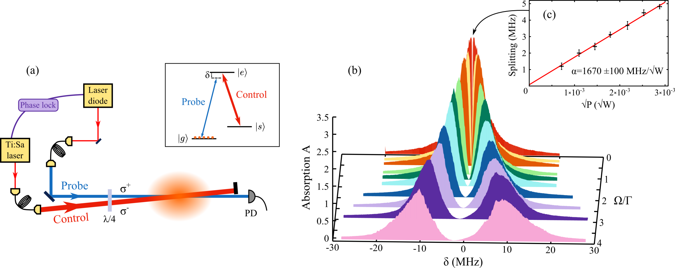
Figure 1: (color online). Absorption in a $\Lambda$-type system. (a) Experimental setup: a weak probe beam and a control beam travel through a cloud of cold cesium atoms. Atoms are initially in the ground state $|g\rangle$. The probe field is close to the $|g\rangle\rightarrow|e\rangle$ transition (detuning $\delta$) while the control field drives the $|s\rangle\rightarrow|e\rangle$ transition on resonance; PD : high-gain photodiode. (b) Absorption profiles are displayed as a function of the detuning $\delta$ for a control Rabi frequency $\Omega$ between $0.1\Gamma$ and $4\Gamma$, where $\Gamma$ is the natural linewidth. (c) Experimental splitting as a function of $\sqrt{P}$, where $P$ is the measured control power, fitted by a linear function.

The experimental setup is illustrated in Fig. 1(a). The optically thick atomic ensemble is obtained from cold cesium atoms in a magneto-optical trap (MOT). The three-level $\Lambda$ system involves the two ground states, $|g\rangle=|6S_{1/2},F=3\rangle$ and $|s\rangle=|6S_{1/2},F=4\rangle$, and one excited state $|e\rangle=|6P_{3/2},F=4\rangle$. The control field is resonant with the $|s\rangle$ to $|e\rangle$ transition, while the probe field is scanned around the $|g\rangle$ to $|e\rangle$ transition, with a detuning $\delta$ from resonance.

Each run of the experiment involves a period for the cold atomic cloud to build up and a period for measurement. This sequence is repeated every 25 ms and controlled with a FPGA board. After the build-up of the cloud in the MOT, the current in the coils generating the trapping magnetic field and then the MOT trapping beams are switched off. In order to transfer the atoms from the $|s\rangle$ to the $|g\rangle$ ground state, the MOT is illuminated with a $\sigma^{-}$-polarized 1 ms-long depump pulse with a power of 900 $\mu$W and resonant with the $|s\rangle$ to $|e\rangle$ transition. After this preparation stage, the optical depth at resonance for atoms in $|s\rangle$ is zero within our experimental precision. The remaining spurious magnetic fields have been canceled down to 5mG using a RF spectroscopy technique.

The measurement period starts 3 ms after the extinction of the MOT magnetic field. The atomic ensemble is illuminated with a 30 $\mu$s-long control pulse and a probe pulse lasting 15 $\mu$s is sent during this time. The probe field is emitted by an extended cavity grating stabilized laser diode, whereas the control field is generated by a Ti:Sapphire laser locked on resonance using saturated absorption spectroscopy. The two lasers are phase-locked. The control field is $\sigma^{-}$-polarized, with a 200 $\mu$m waist in the MOT and a 2^∘ angle relative to the direction of the probe beam. The probe field is $\sigma^{+}$-polarized, with a waist of 50 $\mu$m and a power of 30 nW. To measure absorption profiles, the probe beam frequency is swept over a few natural linewidths by changing the locking frequency point. Its absorption is measured with a high-gain photodiode. The optical depth in the $|g\rangle$ state is chosen to be around 3 to avoid any profile shape distortion due to the limited dynamic range of the photodiode.

Figure 1(b) gives the absorption of the probe field, $A=\textrm{ln}(I_{\textrm{ref}}/I)$, as a function of its detuning $\delta$ from resonance for different values of the control power (0.1 to 200 $\mu$W), i.e. for different values of the control Rabi frequency $\Omega$. The quantity $I_{\textrm{ref}}$, which gives the transmission in the absence of atoms, is measured by sending an additional probe pulse when all the atoms are still in the $|s\rangle$ ground state. The Rabi frequency $\Omega$ of the control field is changed from very weak values (at the back) to four times the natural linewidth $\Gamma$ (at the front). Each profile results from an averaging over twenty repetitions of the experiment. The narrow transparency dip appearing for low Rabi frequencies gets wider when the Rabi frequency increases, to finally give two well-separated resonances corresponding to the two excited dressed states.

Let us note that the Rabi frequency $\Omega$ is a linear function of the electric field, and can be expressed as $\Omega=\alpha\,\sqrt{P}$, with $P$ the power of the control field. An effective value of $\Omega$ can be inferred from the experimental splittings (i.e. the distance between the two maxima) observed in the absorption profiles for low-power control field (Fig. 1(c)). For a three-level system this splitting is indeed equal to the Rabi frequency within a very good approximation for low decoherence in the ground state Arimondo . We find $\alpha=1670\pm 100\,\textrm{MHz}/\sqrt{\textrm{W}}$.

We now turn to the detailed analysis of the absorption profiles. For a three-level $\Lambda$ system, to first order in the probe electric field, the atomic susceptibility on the probe transition for a control field on resonance is given by Anisimov :

$$\chi(\delta)=-\frac{n_{g}|d_{eg}|^{2}}{\mathbf{\hbar}\epsilon_{0}}\,\frac{\delta+i\gamma_{gs}}{\delta^{2}-|\Omega_{0}|^{2}/4-\gamma_{eg}\gamma_{gs}+i\delta(\gamma_{eg}+\gamma_{gs})}$$ (1)

${n_{g}}$ stands for the atomic density in state $|g\rangle$ and $d_{eg}$ denotes the electric dipole moment between $|e\rangle$ and $|g\rangle$. Here, the Rabi frequency of the control field is $\Omega_{0}=2\,|d_{es}|\varepsilon_{c}/\hbar$, with $\varepsilon_{c}$ the amplitude of the positive frequency part of the control field. The optical coherence relaxation rate is $\gamma_{eg}=\Gamma/2$ where $\Gamma/2\pi=5.2$ MHz. $\gamma_{gs}$ is the dephasing rate of the ground state coherence, $\gamma_{gs}=10^{-2}\Gamma$ in our experimental case.

Depending on the value of the control Rabi frequency $\Omega_{0}$, Eq. 1 can be rewritten in different ways Anisimov ; Salloum ; Zhang . For Rabi frequencies $\Omega_{0}<\Omega_{t}=\gamma_{eg}-\gamma_{gs}$, the spectral poles of the susceptibility are imaginary. Then, the linear absorption $A\propto\textrm{Im}[\chi]$ can be expressed as the difference between two Lorentzian profiles centered at zero frequency, a broad one and a narrow one. For $\Omega_{0}>\Omega_{t}$, this decomposition is not possible anymore. For large Rabi frequencies, $\Omega_{0}\gg\Gamma$, Eq. 1 can be written as the sum of two well separated Lorentzian profiles with similar widths. Absorption profiles for these two model can thus be written as:

$$A_{\textrm{EIT}} =\frac{C_{+}}{1+(\delta-\epsilon)^{2}/(\gamma_{+}^{2}/4)}-\frac{C_{-}}{1+\delta^{2}/(\gamma_{-}^{2}/4)}$$ (2)

$$A_{\textrm{ATS}} =\frac{C_{1}}{1+(\delta+\delta_{1})^{2}/(\gamma_{1}^{2}/4)}+\frac{C_{2}}{1+(\delta-\delta_{2})^{2}/(\gamma_{2}^{2}/4)}$$ (3)

where $C_{+}$, $C_{-}$, $C_{1}$, $C_{2}$ are the amplitudes of the Lorentzian curves, $\gamma_{+}$ and $\gamma_{-}$, $\gamma_{1}$ and $\gamma_{2}$ are their widths, $\epsilon$, $\delta_{1}$ and $\delta_{2}$ are their shifts from zero frequency. Equation 2 describes a Fano interference and corresponds to the EIT model, while Eq. 3 corresponds a strongly-driven regime with a splitting of the excited state, i.e. ATS.

For a three-level system, the various parameters introduced in the two above expressions can be calculated from Eq. 1. Conversely, in our experimental system, we use functions $A_{\textrm{EIT}}$ and $A_{\textrm{ATS}}$ to fit the experimental absorption curves, adjusting all the aforementioned parameters. The test proposed in Sanders2011 aims at determining which of these generic models is the most likely for given experimental data.

Figure 2 shows the measured probe absorption as a function of the detuning $\delta$ (blue dots) together with the fits to $A_{\textrm{EIT}}$ (red curves) and $A_{\textrm{ATS}}$ (green curves). A low value of the control Rabi frequency, $\Omega=0.2\Gamma$ is shown in panel (a), and a larger one, $\Omega=2.3\Gamma$ in panel (b). Let us note that for the EIT model a detuning parameter $\epsilon$ was introduced between the atomic line center and the EIT dip to account for a possible experimental inaccuracy in the frequency locking reference of the lasers. For the ATS model the parameters describing each Lorentzian curve are independent of each other (contrary to what would be deduced from Eq. 1) in order to account for their experimentally different widths and heights. These asymmetries are discussed below. As expected, the EIT model fits better the low-power control field region (panel (a)) while the ATS model fits better the strong-power control field region (panel (b)).

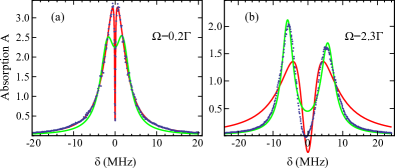
Figure 2: (color online). Absorption profiles and model fits for two values of the control Rabi frequency $\Omega$. Experimental data (blue dots) are presented together with the best fits of functions $A_{\textrm{EIT}}(C_{+},C_{-},\epsilon,\gamma_{+},\gamma_{-})$ (red solid lines) and $A_{\textrm{ATS}}(C_{1},C_{2},\delta_{1},\delta_{2},\gamma_{1},\gamma_{2})$ (green solid lines). Parameters $C_{+},C_{-},C_{1},C_{2}$ representing the amplitudes of the absorption curves are in dimensionless units, while the parameters $\epsilon,\gamma_{+},\gamma_{-}$ and $\delta_{1},\delta_{2},\gamma_{1},\gamma_{2}$ representing detunings and widths are in MHz. (a) $\Omega=0.2\Gamma$. In this case $A_{\textrm{EIT}}(3.52,3.14,1.45\times 10^{-2},5.71,0.239)$ fits the experimental data much better than $A_{\textrm{ATS}}(2.01,2.04,1.84,1.84,4.14,4.08)$. (b) $\Omega=2.3\Gamma$. Here $A_{\textrm{ATS}}(2.05,1.64,5.86,5.67,3.94,4.68)$ fits the data better than $A_{\textrm{EIT}}(1.59\times 10^{5},1.59\times 10^{5},1.45\times 10^{-7},8.17,8.17)$.

As proposed in Sanders2011 , in order to quantitatively test the quality of these model fits, we then calculate the Akaike information criterion (AIC) Akaike . This criterion, directly provided by the function NonLinearModelFit in Mathematica, is equal to $I_{j}=2k-\textrm{ln}(L_{j})$ where $k$ is the number of parameters used and $L_{j}$ the maximum of the likelihood function obtained from the considered model, labeled with $j$ ($j=\textrm{EIT}$ or ATS). The relative weights $w_{\textrm{EIT}}$ and $w_{\textrm{ATS}}$ that give the relative probabilities of finding one of the two models can be calculated from these quantities and are given by:

$$w_{\textrm{EIT}}=\dfrac{e^{-I_{\textrm{EIT}}/2}}{e^{-I_{\textrm{EIT}}/2}+e^{-I_{\textrm{ATS}}/2}},\,\,w_{\textrm{ATS}}=1-w_{\textrm{EIT}}.$$

These weights are plotted in Fig. 3 (curves (1) and (2)), as a function of the experimentally determined Rabi frequency. They exhibit a binary behavior. They are close to 0 or 1 and there is an abrupt transition from EIT model to ATS model.

Figure 3: (color online). Experimental Akaike weights $w_{j}$ as a function of the Rabi frequency $\Omega$ for ATS model (green triangles, curve (1)) and for EIT model (red triangles, curve (2)). Experimental per-point weights $\overline{w}_{j}$ for ATS model (green dots, curve (3)) and for EIT model (red dots, curve (4)). The grey area indicates the EIT/ATS model transition. Error bars include the uncertainty on the coefficient $\alpha$ and on the measured power. The solid lines give the theoretical per-point weights for a pure 3-level system (curves (5) and (6)).

We then investigate the second criterion proposed in Ref. Sanders2011 , also based on Akaike’s information criterion but with a mean per-point weight $\overline{w}$. It can be obtained by dividing $I_{j}$ by the number of experimental points N. The weights for the EIT and the ATS models are now given respectively by

$$\overline{w}_{\textrm{EIT}}=\dfrac{e^{-I_{\textrm{EIT}}/2N}}{e^{-I_{\textrm{EIT}}/2N}+e^{-I_{\textrm{ATS}}/2N}},\,\,\overline{w}_{\textrm{ATS}}=1-\overline{w}_{\textrm{EIT}}.$$

The resulting curves are presented in Fig. 3 (curves (3) and (4)). Starting from a per-point weight equal to 0.5 for both models in the absence of control field (the two models are equally likely), the EIT model first dominates in the low Rabi frequency region. Then the likelihood of the EIT model decreases and a crossing is observed for the same value as for the previous criterion. The ATS model then dominates for larger Rabi frequency, as expected.

For the Akaike weights, as well as for the per-point weights, the behavior is in good qualitative agreement with the predictions given in Ref. Sanders2011 and with our simulations for a three-level system. However, the transition between the two models is obtained experimentally for $\Omega/\Gamma=1.23\pm 0.10$, while a value of $\Omega/\Gamma=0.91$ is obtained for the per-point weights of a pure three-level system, calculated for the same Rabi frequencies, as shown in Fig. 3 (solid grey lines). Moreover, for large Rabi frequencies the per-point weights corresponding to ATS and EIT saturate at 0.7 and 0.3 respectively instead of going to 1 and 0 as in the theoretical three-level model. For low Rabi frequencies, the shape of the curves also differs significantly. These various features suggest that the system cannot be described by a simple three-level model. Below, we proceed to theoretical simulations including additional parameters that influence the ATS/EIT model transition and the general shape of the per-point weight curves.

First, we take into account the other hyperfine sublevels of the $6P_{3/2}$ manifold, based on a previous theoretical model Oxy2011 ; Michael2012 . We find that these contributions explain the asymmetry between the two dressed-state resonances observed in Fig. 2(b) at large Rabi frequencies but they do not significantly influence the per-point weight curves. The latter are shown in Fig. 4(b) (solid lines), with a crossing point for $\Omega/\Gamma=0.91$.

We then consider the effect of the Zeeman structure. Several Zeeman sublevels are involved in each atomic level as shown in Fig. 4(a). We have determined the atomic distribution in the Zeeman sublevels from the optical pumping due to the depump field (Fig. 4(a), inset). Since the control and probe fields have opposite circular polarizations, we can consider that the atomic scheme is a superposition of six independent $\Lambda$ subsystems with different Rabi frequencies. The susceptibility is calculated as the sum of the corresponding susceptibilities. The per-point weights for theoretical absorption curves calculated from this model (including the hyperfine structure) are shown in Fig. 4(b) (dotted lines). For the horizontal axis, as the system does not have a single Rabi frequency, we have used an effective Rabi frequency obtained from the splitting between the maxima of the theoretical absorption curves. The transition point is found for $\Omega/\Gamma=0.98$, close to the value obtained for a three-level system. These simulations show that taking into account the Zeeman sublevels does not lead to a large enough alteration of the crossing point as compared to the three-level model. However a significant change in the values of the per-point weights for large Rabi frequencies is obtained for the model including the Zeeman sublevels, and it is comparable to the experimental one.

We finally include a residual inhomogeneous Doppler broadening $\Gamma_{D}$. By fitting the experimental absorption profile in the absence of control field, we obtain $\Gamma_{D}/2\pi=0.6$ MHz. The per-point weights for theoretical absorption curves including this residual broadening are given in Fig. 4(b) (dashed lines). The crossing point is found for a value $\Omega/\Gamma=1.05$, which is in better agreement with the experimental value. The slightly larger value of the experimental transition point is very likely to be due to heating and additional broadening caused by the control laser. If we assume an inhomogeneous broadening $\Gamma_{D}/2\pi=1.3$ MHz (dash-dotted lines), the per-point weights for the theoretical absorption curves cross each other for $\Omega/\Gamma=1.23$. Moreover the shape of the curves including even a small Doppler broadening agrees much better with the experimental results for the low control Rabi frequency region. Thus, including in the model both the Zeeman structure of the atomic system and a residual Doppler broadening due to the finite temperature of the atoms allows us to explain the observed experimental behaviour when the EIT-ATS discrimination criterion is applied.

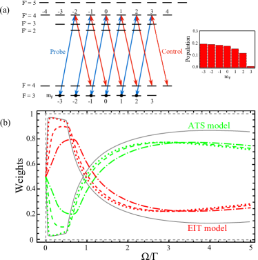
Figure 4: (color online). Theoretical simulations with Zeeman sublevels and Doppler broadening. (a) Level scheme for the Cs $D_{2}$ line and the six three-level transitions involving Zeeman sublevels; inset: population distribution. (b) Per-point weights for a three-level system (grey solid lines), for a system involving Zeeman sublevels (dotted lines), for a system involving Zeeman sublevels and residual Doppler broadenings $\Gamma_{D}/2\pi=0.6$ MHz (dashed lines) and $\Gamma_{D}=1.3/2\pi$ MHz (dash-dotted lines).

In summary, we have tested and analyzed in detail the transition from the ATS model to the EIT model proposed in Ref. Sanders2011 in a well controlled experimental situation. The criteria have been calculated and give a consistent conclusion for discerning between the two regions. The observed differences from the three-level model have been interpreted by a refined model taking into account the specific level structure and some residual inhomogeneous broadening. This study confirms the sensitivity of the proposed test to the specific properties of the medium and opens the way to a new tool for characterizing complex systems involving coherent processes.

- (1) M. Fleischhauer, A. Imamoğlu, and J. P. Marangos, Rev. Mod. Phys. 77, 633 (2005).
- (2) G. Alzetta et al., Nuovo Cimento 36, 5 (1976).
- (3) E. Arimondo, Coherent Population Trapping in Laser Spectroscopy, Prog. Opt. Vol. 5 (Elsevier, Amsterdam, 1996), pp. 257-354.
- (4) S. E. Harris, J. E. Field, and A. Imamoğlu, Phys. Rev. Lett. 64, 1107 (1990).
- (5) K.-J. Boller, A. Imamoğlu, and S. E. Harris, Phys. Rev. Lett. 69, 2593 (1991).
- (6) J. P. Marangos, J. Mod. Opt. 45, 471 (1998).
- (7) A. I. Lvovsky, B. C. Sanders, and W. Tittel, Nature Photon. 3, 706 (2009).
- (8) L. V. Hau, S. E. Harris, Z. Dutton, and C. H. Behroozi, Nature 397, 594 (1999).
- (9) W.R. Kelly et al., Phys. Rev. Lett. 104, 163601 (2010).
- (10) A. H. Safavi-Naeini et al., Nature 472, 69 (2011).
- (11) U. Fano, Phys. Rev. 124, 1866 (1961).
- (12) S. Harris, Phys. Today 50, 36 (1997).
- (13) S. H. Autler and C. H. Townes, Phys. Rev. 100, 703 (1955).
- (14) C. Cohen-Tannoudji and S. Reynaud, J. Phys. B 10, 2311 (1977).
- (15) C. Cohen-Tannoudji, J. Dupont-Roc, and G. Grynberg, Atom-Photon Interactions: Basic Processes and Applications (Wiley Interscience, New York, 1992).
- (16) P. Anisimov and O. Kocharovskaya, J. Mod. Opt. 55, 3159 (2008).
- (17) T. Y. Abi-Salloum, Phys. Rev. A 81, 053836 (2010).
- (18) Z. H. Li, Y. Li, Y. F. Dou, and J. X. Zhang, Chin. Phys. B 21, 3012 (2012).
- (19) P. M. Anisimov, J. P. Dowling, and B. C. Sanders, Phys. Rev. Lett. 107, 163604 (2011).
- (20) K. P. Burnham and D. R. Anderson, Model Selection and Multimodel Inference (Springer-Verlag, New York, 2002), 2nd edition.
- (21) O. S. Mishina et al., Phys. Rev. A 83, 053809 (2011).
- (22) M. Scherman et al., Opt. Express 20, 4346 (2012).