Giant number fluctuations in microbial ecologies

Abstract

Statistical fluctuations in population sizes of microbes may be quite large depending on the nature of their underlying stochastic dynamics. For example, the variance of the population size of a microbe undergoing a pure birth process with unlimited resources is proportional to the square of its mean. We refer to such large fluctuations, with the variance growing as square of the mean, as Giant Number Fluctuations (GNF). Luria and Delbrück showed that spontaneous mutation processes in microbial populations exhibit GNF. We explore whether GNF can arise in other microbial ecologies. We study certain simple ecological models evolving via stochastic processes: (i) bi-directional mutation, (ii) lysis-lysogeny of bacteria by bacteriophage, and (iii) horizontal gene transfer (HGT). For the case of bi-directional mutation process, we show analytically exactly that the GNF relationship holds at large times. For the ecological model of bacteria undergoing lysis or lysogeny under viral infection, we show that if the viral population can be experimentally manipulated to stay quasi-stationary, the process of lysogeny maps essentially to one-way mutation process and hence the GNF property of the lysogens follows. Finally, we show that even the process of HGT may map to the mutation process at large times, and thereby exhibits GNF.

1 Introduction

The presence of huge statistical fluctuations in microbial populations was first shown in a simple biological process, namely the birth or autocatalytic process that involves the binary fission of a cell into two genetically identical daughters. The full mathematical solution of the stochastic process with the exact distribution of the population number, and in particular the variance, was calculated by Delbrück (1940). In such a process the mean of the population number $n(t)$ grows exponentially with time $t$ as: $\langle n(t)\rangle=n(0)\exp(\beta t)$, where $\beta$ is the birth rate, and the variance $Var[n(t)]=\langle n(t)\rangle^{2}/n(0)-\langle n(t)\rangle$, which grows as square of the mean at large times. Due to such huge fluctuations this process stands in direct contrast with the familiar Poisson process which has $Variance=mean$. In this paper, we refer to the statistically large fluctuations characterized by $Variance\sim(mean)^{\nu}$ with $\nu=2$, as ‘giant number fluctuations’ (GNF). This term has been appeared previously in other contexts like spatial fluctuations of bacterial numbers (Zhang et al., 2009, 2010), where $\nu>1$ has been regarded as a signature of large fluctuations than usual. Here, since we use the pure birth process as a reference case to compare with other ecological models, by GNF we specifically mean that the power $\nu=2$. The GNF property continues to hold even for a more complicated process, namely spontaneous forward mutation, as revealed by the classic work of Luria and Delbrück (1943).

The work of Luria and Delbrück (1943) (henceforth LD) in which a bacterial population in a nutrient-rich medium was allowed to grow for a while, and then subjected to an one-time attack of a lethal virus, was important in many ways. Their work provided evidence for spontaneous random mutations in the DNA sequence of the genome (Alberts et al., 2002) and also initiated a practical experimental approach to calculate the mutation rate (Rosche and Foster, 2000). A key result of their work was the demonstration of GNF in the number $x(t)$ of the mutant bacteria at large times — $Var[x(t)]\sim\langle x(t)\rangle^{2}$. It is important to note that GNF in the LD ecological model does not trivially follow from the results of a pure birth process. The mutant number in an LD ecological model and the bacterial number in a pure birth process have distinct distribution functions — the former has a power law tail (Mandelbort, 1974; Ma et al., 1992; Qi Zheng, 1999), while the latter has an exponential tail (Delbrück, 1940). Moreover the GNF property holds at large times, and not at early times, in both the LD and the birth processes. The LD model involves three processes altogether, namely the birth process of the wildtype bacteria, that of its mutant, and the mutation process. Luria and Delbrück (1943) treated the two birth processes deterministically while the mutations were treated as random events. Lea and Coulson (1949) improved the latter by also treating the birth of mutants stochastically. Finally Bartlett (Armitage, 1952; Qi Zheng, 1999, pg. 23) obtained the most realistic calculations by treating all the three processes as stochastic. While all three formulations yield different distribution functions, the GNF property holds asymptotically for all of them. The LD result motivates us to explore the prevalence of the GNF property in other microbial ecologies.

In a general microbial ecology, where complex inter-microbe interactions are involved, one may ask: what is the relationship between the variance and the mean of a particular species? In this paper we study the asymptotic population dynamics of three progressively more complex ecological models (as compared to the original LD case) namely (i) a model involving bi-directional mutation process, (ii) a particular limit of infection of bacteria by bacteriophage and (iii) two simple models of horizontal gene transfer.

In the bi-directional mutation, bacteria not only mutate by a forward mutation like the LD case, but the mutant can convert back to the original wildtype bacteria (Lieb, 1951). Such reverse mutations are well known and in fact form the basis of the Ames test which is one of the standard tests for determining the mutagenicity of chemicals (McCann et al., 1975; Mortelmans and Zeiger, 2000). We show analytically exactly that the asymptotic distribution of population sizes of both the wildtype and the mutant obeys the GNF relationship.

In nature, temperate bacteriophages (for example, phage $\lambda$ which infects E. Coli) can follow either one of two life cycles (Sneppen and Zocchi, 2005; Court et al., 2007). In the lytic life cycle, the phage that infects the host cell multiplies through replication and ultimately bursts out by killing the bacterium. In the lysogenic life cycle the phage combines its genome with that of the bacterium to form a stable lysogen (Kourilsky, 1973; Weitz et al., 2008; Wang and Goldenfeld, 2010; Zeng et al., 2010). Interestingly, we show that if experimentally the phage population size can be controlled to stay quasi-constant, this three-species system reduces to an one-way mutation process involving two species. We numerically demonstrate this LD like behavior and the associated GNF property for our proposed protocol.

Finally we study ecological models involving horizontal gene transfer (HGT). HGT occurs due to exchange of DNA segments of a genome between different strains of bacteria, and can take place by means of three known mechanisms, namely transformation, transduction, or conjugation. The discovery of HGT as an important inter-microbe interaction over the past few decades has led to a resurgence of interest in microbial evolutionary dynamics (Ochman et al., 2000; Chen et al., 2005; Babić et al., 2008; Goldenfeld and Woese, 2007). Here we have found that ecological models involving bacterial genotypes undergoing mutual HGT, may sometimes map to mutation processes at large times. We numerically demonstrate the appearance of GNF in two- and four-species HGT models.

In all the ecological models we study in this paper, we assume a nutrient-rich environment (like the experimental conditions of Luria and Delbrück), so that unrestricted birth is possible for each population for indefinite time. Although in a natural environment the exponential phase (often also called the “logarithmic phase”) of the bacterial growth may approach saturation due to overcrowding and limited food resources, in a controlled laboratory experiment one can replenish nutrients to prolong the exponential phase (see Lieb, 1951). The curious reader may wonder whether the GNF property holds beyond the exponential growth phase or not. We will discuss below the case of a birth process with “limited resources” and deaths, and show that fluctuations are ordinary Poisson-like as saturation is reached.

Experiments that study microbial populations in the presence of unknown interactions among the different genotypes may therefore look for GNF. The prevalence of the GNF property in the systems that we study, suggests, that it is likely to be found often in the laboratory.

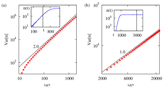
Figure 1: The number fluctuations in the exponential phase and saturation phase of the logistic birth model are compared. (a) Log-log plot of $Var[n]\sim\langle n\rangle^{2}$ in the exponential phase, with $\langle n\rangle\sim\exp((\beta-\delta)t)$ (see inset), and (b) log-log plot $Var[n]\sim\langle n\rangle$ in the saturation phase, with $\langle n\rangle\sim K$ (see inset). Note $\beta=0.02$, $\delta=0.01$, $n(0)=10$, and for the two insets $K=50000$. Every data point (circles) of both (a) and (b) is obtained by averaging over $10^{5}$ independent histories. The data points in (a) are obtained at different chosen time $t$ for a fixed $K=50000$, while those in (b) are obtained at different chosen values of $K$ for a fixed time $t=3000$ which is deep inside the saturation (see inset).

2 Birth and bi-directional mutation processes

2.1 Birth process

The process by which a bacterial species multiplies by successive division is stochastic. In the presence of unlimited resources it is represented as: $N\stackrel{{\scriptstyle\beta}}{{\rightarrow}}N+N$, where $\beta$ is the birth rate. The probability $P_{n}(t)=Prob.[n(t)=n]$ of the random population size $n(t)$ at any time $t$ is governed by the Master quation:

$$\frac{\partial P_{n}(t)}{\partial t} = \beta(n-1)P_{n-1}(t)-\beta nP_{n}(t)$$ (1)

The exact distribution $P_{n}(t)$ was solved by Delbrück (1940) and that leads to: $Var[n]=\langle n\rangle^{2}/n(0)-\langle n\rangle$. At large times, $Var[n]\sim\langle n\rangle^{2}$, which is the GNF property.

In the presence of limited resources the bacterial population size is expected to saturate. Does the GNF property hold in the saturation phase? A standard model of microbial growth under nutrient-limiting conditions is the logistic growth model, where population numbers eventually saturate due to limited resources. We studied a stochastic version of the logistic growth model (Tan and Piantadosi, 1991) represented by the following processes:

$$R_{1}: ~{}~{}N\stackrel{{\scriptstyle\beta(1-n/K)}}{{\xrightarrow{\hskip 22.76228pt}}}N+N$$

$$R_{2}: ~{}~{}N\stackrel{{\scriptstyle\delta}}{{\longrightarrow}}0$$ (2)

Here, the parameter $K$ is called the ‘carrying capacity’ and represents the maximal population that can be supported by the available resources. Note that the birth rate $\beta^{{}^{\prime}}\equiv\beta(1-n/K)$ is not constant. The inclusion of death (reaction $R_{2}$ in Eq. (2)) is important — without it the evolution in the saturation phase would stall as $n(t)\rightarrow K$ (and $\beta^{{}^{\prime}}\rightarrow 0$). The Master equation of this process is non-linear in population size:

$$\frac{\partial P_{n}(t)}{\partial t} = \beta(1-(n-1)/K)(n-1)P_{n-1}(t)+\delta(n+1)P_{n+1}(t)$$ (3)

$$-(\beta(1-n/K)+\delta)nP_{n}(t)$$

We simulate Eq. 2 using kinetic Monte-Carlo (Bortz et al., 1975; Gillespie, 1976, 2007) and the results for $Var[n]=\langle n^{2}\rangle-\langle n\rangle^{2}$ in the exponential and saturation phases of the system, are shown in Fig. 1(a) and 1(b), respectively. While (a) shows GNF, (b) shows $Var[n]\sim\langle n\rangle$. In this model, a small proportion of the stochastic histories lead to extinctions of the population ( $\sim 0.1\%$ for $K=5000$ for example). We obtain $Var[n]$ by doing a history average over cultures which do not become extinct, starting from a fixed $n(0)$. The result in Fig. 1(b) shows that the giant fluctuations which arise in the exponential growth phase, diminish and become ordinary Poisson-like in the saturation regime.

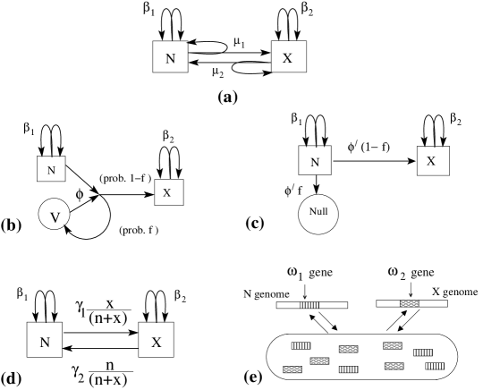
Figure 2: The schematic diagrams of the ecological models. The double arrows going up from a population (marked by $\beta_{1}$ or $\beta_{2}$) represent the birth processes. (a) Bi-directional mutation. (b) Lysis-Lysogeny. (c) The LD limit of the Lysis-Lysogeny model with constant viral population. (d) Two species HGT. (e) Visualization of the two species HGT mechanism via a shared gene pool.

2.2 Bi-directional mutation

In this section we calculate the moments of the population sizes of species involved in a bi-directional mutation process. We follow the method of Bertlett (pg. 34–40 Armitage, 1952; Bertlett, 1978; Qi Zheng, 1999, pg. 23) in which the mutation process is assumed to produce a mutant and a normal cell from a normal cell (formulation (B) of D. G. Kendall, (see Qi Zheng, 1999, pg. 4)). In nature there exists a possibility of an occasional reverse mutation that takes the microbe to the original genotype (Lieb, 1951), thereby diminishing the population of the mutant pool. The studies on spontaneous forward and reverse mutation of different bacterial genotypes have revealed that the latter two rates may differ by a factor of $10-100$ in magnitude (Bunting, 1946; Lieb, 1951). Let the wildtype population be denoted by $N$ (with a population size $n(t)$). The mutant population $X$ (with a population size $x(t)$) can convert back to the wildtype population $N$ (see Fig. 2a) via the reaction channel $R_{4}$ in Eq. (4), which makes the problem two-way coupled. The reactions are:

$$R_{1}: ~{}~{}N\stackrel{{\scriptstyle\beta_{1}}}{{\rightarrow}}N+N$$

$$R_{2}: ~{}~{}X\stackrel{{\scriptstyle\beta_{2}}}{{\rightarrow}}X+X$$

$$R_{3}: ~{}~{}N\stackrel{{\scriptstyle\mu_{1}}}{{\rightarrow}}N+X$$

$$R_{4}: ~{}~{}X\stackrel{{\scriptstyle\mu_{2}}}{{\rightarrow}}N+X.$$ (4)

Here $\beta_{1}$ and $\beta_{2}$ are the bare birth rates of the wildtype and mutant population respectively, and $\mu_{1}$ and $\mu_{2}$ are the forward and the reverse mutation rates respectively.

We begin by considering the joint probability distribution $P_{n,x}(t)=Prob.[n(t)=n;x(t)=x]$. From the rates given in Eq. (4), the master equation is as follows:

$$\frac{\partial P_{n,x}(t)}{\partial t} = \beta_{1}(n-1)P_{n-1,x}(t)+\beta_{2}(x-1)P_{n,x-1}(t)+\mu_{1}nP_{n,x-1}(t)+\mu_{2}xP_{n-1,x}(t)$$ (5)

$$-(\beta_{1}n+\beta_{2}x+\mu_{1}n+\mu_{2}x)P_{n,x}(t)$$

The above equation can be solved analytically exactly for its moments using the generating function technique (see A). We find that the means of both $N$ and $X$ populations follow the same time development at asymptotically large times (see Eq. 16 in Appendix A):

$$\langle n\rangle\sim\langle x\rangle\sim e^{\alpha_{1}t},~{}~{}\text{where,}~{}\alpha_{1}=[(\beta_{1}+\beta_{2})+\sqrt{(\beta_{1}-\beta_{2})^{2}+4\mu_{1}\mu_{2}}]/2$$ (6)

Thus the bi-directional coupling makes the wildtype and mutant track each other in perfect synchrony. The effective growth rate $\alpha_{1}$ of the two species is a complicated combination of all the rates defining the ecological model. Turning to the fluctuations (see Eq. 16 in Appendix A), we find that mathematically the largest exponent contributing to the variance is such that at large $t$:

$$Var[n]\sim Var[x]\sim e^{2\alpha_{1}t}.$$ (7)

Thus the GNF property holds: $Var[n]\sim\langle n\rangle^{2}$ and $Var[x]\sim\langle x\rangle^{2}$. We note that this GNF property holds as long as there is no saturation.

3 LD limit of Lysis-Lysogeny

The prolonged co-evolution of temperate phage with a bacterial population can be modeled as a stochastic process wherein virus-infected bacteria either die by lysis, or transform into another genotype via lysogeny (Sneppen and Zocchi, 2005; Court et al., 2007). A large number of virus particles are born during lysis. The classic host-phage system of the bacteria E. Coli and phage $\lambda$ exhibits the processes of lysis and lysogeny (Zeng et al., 2010). This ecology can be modeled by the following reactions (see Fig. 2b):

$$R_{1}: ~{}~{}N\stackrel{{\scriptstyle\beta_{1}}}{{\rightarrow}}N+N$$

$$R_{2}: ~{}~{}N+V\stackrel{{\scriptstyle\phi f}}{{\longrightarrow}}\alpha V$$

$$R_{3}: ~{}~{}N+V\stackrel{{\scriptstyle\phi(1-f)}}{{\xrightarrow{\hskip 22.76228pt}}}X$$

$$R_{4}: ~{}~{}X\stackrel{{\scriptstyle\beta_{2}}}{{\rightarrow}}X+X$$ (8)

Here $N$, $V$ and $X$ denote the sensitive bacteria, the virus particles, and the lysogenic bacteria that is immune to the virus respectively, and $n(t)$, $v(t)$, and $x(t)$ are their respective population sizes. The sensitive bacteria grows at rate $\beta_{1}$. The viral infection rate, i.e. the rate of a $V$ interacting with an $N$, is $\phi$. After infection, the probability of lysis is $f$ and that of lysogeny is $(1-f)$. On lysis, the bacterium dies and the number of viruses released is $\alpha$ (the average viral burst size). On lysogeny, a stable new lysogen is formed which grows at a distinct rate $\beta_{2}$. We assume that only one virus infects a bacterium at a time, i.e. the multiplicity of infection (MOI) is one. Recent experiments have shown that the probability of lysogeny is $\approx 0.2$ when the MOI equals one (Zeng et al., 2010), though older experiments had indicated it to be negligible at this MOI (Kourilsky, 1973). One can write the Master equation for the joint probability $P_{n,x,v}(t)=Prob.[n(t)=n;~{}x(t)=x;~{}v(t)=v]$ describing the ecological model in Eq.(8) (see Eq.(17) in Appendix B); but because of it having nonlinear terms, unlike Eqs. (1) and (5) in Sec. (2), it is hard to tackle analytically. We note that in the above we are ignoring the possibilities of delay of infection to lysis, prophage induction and curing of lysogens, and superinfection.

It is well known (Weitz and Dushoff, 2008; Wang and Goldenfeld, 2010) that without a finite carrying capacity of bacteria due to limited resources, a model like in Eq. (8) makes all the sensitive bacteria $N$ go extinct. The reason is that $\alpha$ is typically large (say $\gtrsim 50$), and in a well mixed medium, the viral population increases very fast, and infects and kills all the sensitive bacteria, leaving the lysogens alive which continue to replicate on their own. Apart from finite carrying capacity, another way to sustain this model ecology is to make the viral population size $v(t)$ constant by some means. This cannot be done in an exact sense, because that would require viral bursts to stop. But this may be done in an approximate way by a plausible experimental protocol that involves replacing part of the culture media by fresh media (see Appendix C).

If the viral population is kept fixed, under the condition $v(t)=constant$, the model defined by Eq. (8) reduces to a two-species model (see Fig. 2c) represented by

$$R_{1}: ~{}~{}N\stackrel{{\scriptstyle\beta_{1}}}{{\rightarrow}}N+N$$

$$R_{2}: ~{}~{}N\stackrel{{\scriptstyle\phi^{{}^{\prime}}f}}{{\longrightarrow}}0$$

$$R_{3}: ~{}~{}N\stackrel{{\scriptstyle\phi^{{}^{\prime}}(1-f)}}{{\xrightarrow{\hskip 22.76228pt}}}X$$

$$R_{4}: ~{}~{}X\stackrel{{\scriptstyle\beta_{2}}}{{\rightarrow}}X+X,$$ (9)

where, $\phi^{{}^{\prime}}=\phi v={\rm constant}$ is a new rate. The above reactions represent an LD-like ecological model with a Master equation given by Eq.(18). The reaction $R_{3}$ in Eq. (9) is like an uni-directional mutation reaction with a mutation rate $\mu^{{}^{\prime}}=\phi^{{}^{\prime}}(1-f)$. Yet the mutation process $N\rightarrow X$ is distinct from the process $N\rightarrow N+X$ used in Berlett’s formulation of mutation (Bertlett, 1978; Qi Zheng, 1999, pg. 23) — they have been referred to as formulations (A) and (B) of D. G. Kendall (see Qi Zheng, 1999, pg. 4) respectively. Apart from this distinction from the LD ecological model, another point of difference is the death of the bacteria $N$ (reaction $R_{2}$). The latter leads to an effective growth rate $\beta_{1}^{{}^{\prime}}\equiv(\beta_{1}-\phi^{{}^{\prime}})$ of $N$. We present the explicit results of the moments of population sizes for Eq. (9) in Eqs. (19) and (20). The results differ from those of the original LD problem only upto the constant prefactors, which do not affect the time dependences. The means and the variances are like LD at large times. Thus for $\beta_{1}^{{}^{\prime}}>\beta_{2}$, $\langle n\rangle\sim\langle x\rangle\sim e^{\beta_{1}^{{}^{\prime}}t}$ and $Var[n]\sim Var[x]\sim e^{2\beta_{1}^{{}^{\prime}}t}$, while for $\beta_{2}>\beta_{1}^{{}^{\prime}}$, $\langle n\rangle\sim e^{\beta_{1}^{{}^{\prime}}t}$, $\langle x\rangle\sim e^{\beta_{2}t}$ and $Var[n]\sim e^{2\beta_{1}^{{}^{\prime}}t}$, $Var[x]\sim e^{2\beta_{2}t}$. Thus in all cases, the GNF property holds at large times, i.e. $Var[n]\sim\langle n\rangle^{2}$ and $Var[x]\sim\langle x\rangle^{2}$, for the lysis-lysogeny model if $v(t)$ is held constant.

We suggest a way to experimentally hold the viral population $v(t)$ quasi-stationary (see Appendix C) by “diluting out” the viruses (Kourilsky, 1973) after equal time intervals $T$. We implement the latter protocol numerically by resetting the viral population number to its initial value $v_{0}$ after each interval $T$. In the meantime over $T$, we time-evolve the population numbers according to the original Lysis-Lysogeny reactions in Eq. (8) using the kinetic Monte-Carlo algorithm (Bortz et al., 1975; Gillespie, 1976, 2007). Thus over a coarse time scale that is greater than $T$, the viral population $v(t)$ is quasi-stationary. We thus find a time window within which this ecological model follows the LD limit.

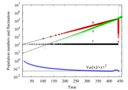
Figure 3: Linear-log plot of $n(t)$, $x(t)$ and $v(t)$ versus time $t$ for a single stochastic history. The fitted exponential functions (solid continuous straight lines) are: $\langle n\rangle\sim 100\times\exp(\beta_{1}^{{}^{\prime}}t)$ (see section 3) and $\langle x\rangle\sim 7\times\exp(\beta_{2}t)$. At the bottom we have $Var[x]/\langle x\rangle^{2}$ which is essentially constant between $t=200-400$, demonstrating the GNF property — for $Var[x]$ and $\langle x\rangle$, averages over $10^{5}$ independent histories were done. The data are for $\beta_{1}=0.02$, $\beta_{2}=0.023$, $\phi=0.00003$, $f=0.8$, $\alpha=50$, $T=0.001$, $n(0)=v(0)=100$ and $x(0)=0$.

We see in Fig. 3 that the data for the instantaneous population sizes $n(t)$ and $x(t)$ of the bacteria and the lysogens, match reasonably well with the growth curves of the means ($\langle n\rangle$ and $\langle x\rangle$) predicted for the LD like problem of Eq. 9. In particular, the fluctuations of the lysogens follow the GNF property as shown in Fig. 3 for large times (within the window $t=200-400$), although not at small times. The time window over which the system behaves like LD may be made larger by choosing a smaller interval $T$. Note that the window is eventually terminated by a sharp catastrophic rise in the viral number as can be seen around $t\sim 450$ in Fig. 3 (for a discussion see Appendix C).

In summary, we have proposed an experimental protocol which can make a stochastically evolving lysis-lysogeny ecology appear as an LD ecology, over a certain time window. As a result, the GNF property of the LD model carries over to this special case of lysis-lysogeny. This GNF property holds only when there is no finite carrying capacity for the populations.

4 Horizontal gene transfer

It is known that HGT produces a high degree of genomic similarity in the interacting microbes (Ochman et al., 2000; Goldenfeld and Woese, 2007). In the spirit of a model studied recently for HGT for four genotypes within a biofilm (Chia et al., 2008) we have constructed a simpler model of HGT involving two bacterial genotypes, $N$ and $X$, with birth rates $\beta_{1}$ and $\beta_{2}$ respectively. Population sizes are denoted by $n(t)$ and $x(t)$. It is assumed that $N$ and $X$ are closely related and they differ at the level of only one gene — $N$ has a gene $\omega_{1}$ and $X$ has a different gene $\omega_{2}$, while the rest of the genome is identical for both. One may think of $N$ and $X$ as the populations of a normal bacterium and an antibiotic resistant variant. The antibiotic resistant bacterium has a mutation in one gene and it can share the mutated gene by HGT and thereby confer antibiotic resistance to the normal bacterium (Akiba et al. (1960); Barlow (2009)). Similarly the normal bacterium can also share its copy of the gene and make the antibiotic resistant bacterium revert back to the normal state. The genomic matters of $N$ and $X$ are exchanged via HGT, transforming one genotype completely into other. This ecological model (see Fig. 2d) is described by the following reactions :

$$R_{1}: ~{}~{}N\stackrel{{\scriptstyle\beta_{1}}}{{\rightarrow}}N+N$$

$$R_{2}: ~{}~{}X\stackrel{{\scriptstyle\beta_{2}}}{{\rightarrow}}X+X$$

$$R_{3}: ~{}~{}N\stackrel{{\scriptstyle\gamma_{1}x/(n+x)}}{{\xrightarrow{\hskip 22.76228pt}}}X$$

$$R_{4}: ~{}~{}X\stackrel{{\scriptstyle\gamma_{2}n/(n+x)}}{{\xrightarrow{\hskip 22.76228pt}}}N$$ (10)

In the above, the processes of HGT are viewed as two-step processes. The genes are exchanged via a communally shared gene-pool (see Fig. 2e). Firstly, a particular species can get a suitable gene from the shared gene pool with a certain probability, which is assumed to be equal to the fraction of its contributor. Thus a gene $\omega_{2}$ contibuted by $X$ is acquired with probability $x/(n+x)$, and $\omega_{1}$ contributed by $N$ is acquired with probability $n/(n+x)$. Secondly, the newly acquired gene is pasted (or overwritten) upon the former one with rates $\gamma_{1}$ and $\gamma_{2}$. Thus the $N$ genome gets transformed into a $X$ genome at an effective rate of $\gamma_{1}x/(n+x)$ ($R_{3}$ in Eq. (10)), while $\gamma_{2}n/(n+x)$ is the effective rate at which $X$ genome gets transformed into a $N$ genome ($R_{4}$ in Eq. (10)); these effective rates are no longer constants like in the LD model and signify that the processes are nonlinear. Since, HGT is a relatively rare event in reality, we further assume $\{\beta_{1},\beta_{2}\}>>\{\gamma_{1},\gamma_{2}\}$ in the subsequent discussion.

One can write the Master equation for the joint probability $P_{n,x}(t)=Prob.[n(t)=n;~{}x(t)=x]$ for the HGT model in Eq. 10 as below:

$$\frac{\partial P_{n,x}(t)}{\partial t} = \beta_{1}(n-1)P_{n-1,x}(t)+\beta_{2}(x-1)P_{n,x-1}(t)$$ (11)

$$+\gamma_{1}[(n+1)(x-1)/(n+x)]P_{n+1,x-1}(t)$$

$$+\gamma_{2}[(n-1)(x+1)/(n+x)]P_{n-1,x+1}(t)$$

$$-(\beta_{1}n+\beta_{2}x+(\gamma_{1}+\gamma_{2})nx/(n+x))P_{n,x}(t)$$

Note that the above Master equation has nonlinear terms unlike Eqs. (1) and (5) in Sec. 2 and is difficult to tackle analytically. One cannot write a system of ODEs for the cumulants in a closed form, and in fact, following similar steps as in Appendix A, every ODE for a cumulant contains the next higher order cumulant. In spite of this difficulty, we will show that the unique algebraic form of non-linearities in the HGT model makes its asymptotic large time limit tractable. At large times, both the populations ($N$ and $X$) are very large and one of them dominates over the other.

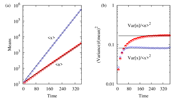
Figure 4: (a) Linear-log plot of $\langle n\rangle$ and $\langle x\rangle$ versus time $t$ for two-species HGT. The data from kinetic Monte-Carlo simulation are shown in symbols. The fitted exponential functions (solid continuous straight lines) are: $\langle n\rangle\sim 12.0\times\exp((\beta_{1}-\gamma_{1}+\gamma_{2})t)$ and $\langle x\rangle\sim 12.0\times\exp(\beta_{2}t)$ (see Sec. 4). (b) Linear-log plot of $Var[n]/\langle n\rangle^{2}$ and $Var[x]/\langle x\rangle^{2}$ versus time $t$ for two-species HGT. The straight lines show that the data is constant at large times. The data in both the curves are for $n(0)=x(0)=10$, $\beta_{1}=0.02$, $\beta_{2}=0.03$, $\gamma_{1}=0.005$ and $\gamma_{2}=0.001$. All data are obtained by averaging over $10^{5}$ independent histories.

We will discuss one case in detail, namely when $X$ dominates over $N$ (i.e. $x>>n$ in Eq. (11)), which occurs for $\beta_{2}>\beta_{1}$ at asymptotically large times. Under this condition, $(x\pm 1)/(n+x)\approx x/(n+x)\approx 1$ in Eq. (11), and one can get an approximate linear Master equation:

$$\frac{\partial P_{n,x}(t)}{\partial t} \approx \beta_{1}(n-1)P_{n-1,x}(t)+\beta_{2}(x-1)P_{n,x-1}(t)+\gamma_{1}(n+1)P_{n+1,x-1}(t)$$ (12)

$$+\gamma_{2}(n-1)P_{n-1,x+1}(t)-(\beta_{1}n+\beta_{2}x+(\gamma_{1}+\gamma_{2})n)P_{n,x}(t)$$

Note that the above Eq. (12) is similar to the Master equation of the LD like ecological model discussed in Appendix B (see Eq. (18)) — they are not exactly identical as the third and fourth terms in the two equations are different. Starting from Eq. (12) we have derived the ODEs of the cumulants and compared them with the Eq. (19) in Appendix B — they are very similar, but not identical. After making the identifications: $\gamma_{1}-\gamma_{2}\equiv\mu^{{}^{\prime}}$, $\beta_{1}-(\gamma_{1}-\gamma_{2})\equiv\beta_{1}^{{}^{\prime}}$ and $\gamma_{1}+\gamma_{2}\equiv\phi^{{}^{\prime}}$, we find that the new ODEs of $\kappa_{1,0}$, $\kappa_{0,1}$ and $\kappa_{2,0}$ in the asymptotic HGT model are same as those of Eq. (19), but ODEs of $\kappa_{1,1}$ and $\kappa_{0,2}$ have minor differences. The latter differences do not change the asymptotic temporal behavior. Solving the ODEs, at large times we get: $\langle n\rangle\sim e^{(\beta_{1}-(\gamma_{1}-\gamma_{2}))t}$, $\langle x\rangle\sim e^{\beta_{2}t}$ and $Var[n]\sim e^{2(\beta_{1}-(\gamma_{1}-\gamma_{2}))t}$, $Var[x]\sim e^{2\beta_{2}t}$ for the parameter regime $\beta_{2}>\beta_{1}>>\gamma_{1}>\gamma_{2}$. Results for other parameter regimes, as well as the opposite case of $n(t)>>x(t)$ will not be discussed, as they are easy to derive following similar steps as above.

Instead of an approximate analysis for large times as above, one may simulate the original exact non-linear model of the HGT process (Eq. (10)) using kinetic Monte-Carlo for all times. We show our data in Fig. 4 — we find a match with the LD like behavior (as predicted from our approximate analysis above) for the means (Fig. 4a). At short times GNF is not seen (Fig. 4b), although the means grow exponentially at those times (see Fig. 4a). As time gets larger, the variances exhibit the GNF property (Fig. 4b) for both $N$ and $X$ populations. Thus we arrive at a conclusion — the two species HGT process approximates a mutation process at large times, due to the algebric uniqueness of its non-linear interaction and has giant fluctuations in its population sizes. Does this conclusion extend to the HGT process involving more than two species? To answer this, we investigate a HGT model involving four genotypes studied by Chia et al. (2008) and confirm that the GNF property holds in this model (see the detailed discussion in Appendix D).

For multiple, i.e. $s$ (with $s\geq 2$) number of species undergoing HGT, the Master equation in general will involve non-linear terms proportional to $(\sum_{i=1}^{r}a_{i}n_{i}/\sum_{i=1}^{s}b_{i}n_{i})\times n_{j}$, where $r<s$, $n_{i}$ is the population size of the $i^{th}$ species, and $\{a_{i},b_{i}\}$ are constants. At large times such non-linear terms may reduce to approximate linear forms for a certain suitable choice of the parameters. This linearization would map the original non-linear processes of HGT to linear mutation processes. As a consequence, an LD like behavior with giant fluctuations may show up in certain parameter regimes of the HGT model with multiple species.

5 Discussion

In this paper, we have studied the property of giant number fluctuation (GNF) in a few interesting microbial ecological models. While this is well-known for the models of the birth process and of uni-directional mutation, we have shown that it also holds for bi-directional mutation, and may be seen under suitable conditions in ecologies of microbes evolving via HGT and Lysis-Lysogeny. In all the ecological models that we have studied, the GNF property appears to arise because the populations effectively obey linear Master equations in population sizes. Yet it is interesting to identify the regimes in these interacting models where the stochastic dynamics resembles the “LD-like” mutation process.

We have shown that whenever an ecological model effectively reduces to a LD-like ecological model at the level of the Master equation, the GNF property follows. In the Lysis-Lysogeny model, given the non-linear terms in the Master equation, making a prediction about GNF becomes difficult. Yet in the special limit when the viral population may be controlled to be quasi-stationary, we see that this process has fluctuation properties like a mutation process. Similarly for the HGT model, the non-linear terms of the Master equation sometimes (and for two-species HGT always) are of an algebraic form that at late times approach linear limiting forms. This again implies an LD like stochastic dynamics with an associated GNF property. The results for the saturation phase of the stochastic logistic birth process, suggest that exponential growth is necessary for seeing GNF. Whether a linearized Master equation involving multiple species would always lead to GNF, remains an open mathematical question to explore in future.

Recently, a similar large fluctuation property has been observed in active matter systems (Zhang et al., 2009, 2010), where the non-equilibrium dynamics of swarming bacteria produces local spatial number fluctuations within a fixed volume, which are non-Poissonian. We would like to comment that in such experiments (Zhang et al., 2010), if the measurements are done over time periods greater than the division time scale (say $\sim 30$ min) of the bacteria, the sources of large fluctuations would be twofold. The first source of this large fluctuation would be non-equilibrium collective dynamics, while the second would be the stochastic microbial population growth itself (as pointed out in this paper). Thus the current work may be of relevance for quantitative studies of microbial systems executing active motion over long times. Apart from that, the GNF in microbial ecologies is not just a mathematical curiosity, but has practical significance. What constitutes an asymptotic regime in practice depends upon the system — it is achieved when the time $t$ is much larger than the inverse of the largest growth rate in the system. For bacteria with a high dividing rate, this may be reached in only a few hours or a day of culture, and the GNF therefore is of practical experimental importance. Luria and Delbrück’s work gave rise to fluctuation assays, where mutation rates are estimated by experimentally determining the distribution of mutants in multiple parallel cultures (Rosche and Foster, 2000). As pointed out in Rosche and Foster (2000), alternate methods based on estimation of the mutant fraction in bacterial cultures are very unreliable due to the presence of GNF. Measurements of quantities that are related to total population numbers of cells in exponential growth are susceptible to such large variances, and more careful analysis of fluctuations may be warranted. Since we have now shown that GNF may arise in other interesting ecological models, more careful analysis of the population sizes in these ecologies need to be done by theorists and experimentalists in future.

Appendix A Details of the calculations for bi-directional mutation

Staring from Eq. (5) in Sec. 2.2, we introduce the probability generating function (p.g.f.) $G(z_{1},z_{2},t)=\sum_{p,q=0}^{\infty}z_{1}^{p}z_{2}^{q}P_{p,q}(t)$, and find its linear partial differential equation (PDE) as below:

$$\frac{\partial G}{\partial t} = \frac{\partial G}{\partial z_{1}}[\beta_{1}z_{1}(z_{1}-1)+\mu_{1}z_{1}(z_{2}-1)]+\frac{\partial G}{\partial z_{2}}[\beta_{2}z_{2}(z_{2}-1)+\mu_{2}z_{2}(z_{1}-1)]$$

Next the cumulant generating function is used, which is defined as $K(\theta_{1},\theta_{2},t)=\ln[G(z_{1}=e^{\theta_{1}},z_{2}=e^{\theta_{2}},t)]=\langle e^{\theta_{1}p+\theta_{2}q}\rangle$. Using this definition we can transform the PDE for $G(z_{1},z_{2},t)$ into a PDE for $K(\theta_{1},\theta_{2},t)$ and then substitute an expansion for $K$, wherein

$$K=\sum_{i+j\geq 1}^{\infty}[(\theta_{1}^{i}\theta_{2}^{j})/(i!j!)]\kappa_{i,j}(t).$$ (14)

Here $\kappa_{i,j}(t)$ are the cumulants of the joint probability distribution. In particular the first few cumulants are given by $\kappa_{1,0}=\langle n\rangle$, $\kappa_{0,1}=\langle x\rangle$, $\kappa_{2,0}=Var[n]$, $\kappa_{0,2}=Var[x]$ and $\kappa_{1,1}=\langle nx\rangle-\langle n\rangle\langle x\rangle$ . Equating the coefficients of $\theta_{1},\theta_{2},\theta_{1}\theta_{2},\theta_{1}^{2}$ and $\theta_{2}^{2}$, we obtain a system of coupled linear ordinary differential equations (ODEs) for the cumulants as below:

$${\kappa^{{}^{\prime}}_{1,0}}(t) = \beta_{1}\kappa_{1,0}+\mu_{2}\kappa_{0,1}$$

$${\kappa^{{}^{\prime}}_{0,1}}(t) = \beta_{2}\kappa_{0,1}+\mu_{1}\kappa_{1,0}$$

$${\kappa^{{}^{\prime}}_{1,1}}(t) = (\beta_{1}+\beta_{2})\kappa_{1,1}+\mu_{1}\kappa_{2,0}+\mu_{2}\kappa_{0,2}$$

$${\kappa^{{}^{\prime}}_{2,0}}(t) = \beta_{1}\kappa_{1,0}+2\beta_{1}\kappa_{2,0}+2\mu_{2}\kappa_{1,1}$$

$${\kappa^{{}^{\prime}}_{0,2}}(t) = (\beta_{2}+\mu_{2})\kappa_{0,1}+2\beta_{2}\kappa_{0,2}+\mu_{1}\kappa_{1,0}+2\mu_{1}\kappa_{1,1}$$ (15)

In above equation, primes denote the ordinary time-derivatives. Note that the linear PDE of p.g.f. $G$ ultimately leads to linear cumulant equations, which is a property of a linear process like the process considered here. Moreover, by putting $\mu_{2}=0$ in Eqs. (LABEL:revmut:3) and (15), we get back the corresponding equations in the original Bertlett’s formulation of the LD model (see Qi Zheng, 1999, pg. 23). Solving the system of ODEs given by Eq. (15) we obtain the means and variances of the populations as follows:

$$\langle n\rangle = A_{1}e^{\alpha_{1}t}+A_{2}e^{\alpha_{2}t}$$

$$\langle x\rangle = B_{1}e^{\alpha_{1}t}+B_{2}e^{\alpha_{2}t}$$

$$Var[n] = C_{1}e^{2\alpha_{1}t}+C_{2}e^{2\alpha_{2}t}+C_{3}e^{\alpha_{1}t}+C_{4}e^{\alpha_{2}t}+C_{5}e^{(\beta_{1}+\beta_{2})t}$$

$$Var[x] = C_{1}^{{}^{\prime}}e^{2\alpha_{1}t}+C_{2}^{{}^{\prime}}e^{2\alpha_{2}t}+C_{3}^{{}^{\prime}}e^{\alpha_{1}t}+C_{4}^{{}^{\prime}}e^{\alpha_{2}t}+C_{5}^{{}^{\prime}}e^{(\beta_{1}+\beta_{2})t}$$

$$\text{where,}~{}\alpha_{1} = [(\beta_{1}+\beta_{2})+\sqrt{(\beta_{1}-\beta_{2})^{2}+4\mu_{1}\mu_{2}}]/2,$$

$$\alpha_{2} = [(\beta_{1}+\beta_{2})-\sqrt{(\beta_{1}-\beta_{2})^{2}+4\mu_{1}\mu_{2}}]/2.$$ (16)

Here $A_{1},\cdots,B_{2}$ and $C_{1},\cdots,C_{5}^{{}^{\prime}}$ are constants involving the parameters $\beta_{1},\beta_{2},\mu_{1},\mu_{2},n(0)$ and $x(0)$. Since in Eq. (16), $\alpha_{1}$ is always greater than $\alpha_{2}$, we arrive at the asymptotic expressions of the means in Eq. (6) of Sec. 2.2. Again, noting that the rate $2\alpha_{1}$ dominates over the other rates $\alpha_{1},\alpha_{2}$, $2\alpha_{2}$ and $(\beta_{1}+\beta_{2})$, appearing in Eq. (16), we get the asymptotic results of the variances in Eq. (7) of Sec. 2.2.

Appendix B Details of the calculations for the Lysis-Lysogeny model

For the Lysis-Lysogeny model defined in Eq. (8), the non-linear Master equation is:

$$\frac{\partial P_{n,x,v}(t)}{\partial t} = \beta_{1}(n-1)P_{n-1,x,v}(t)+\beta_{2}(x-1)P_{n,x-1,v}(t)$$ (17)

$$+\phi f(n+1)(v-\alpha+1)P_{n+1,x,v-(\alpha-1)}(t)$$

$$+\phi(1-f)(n+1)(v+1)P_{n+1,x-1,v+1}(t)$$

$$-(\beta_{1}n+\beta_{2}x+\phi nv)P_{n,x,v}(t)$$

Under the assumption of $v=constant$ the ecological model of Eq. (8) exactly reduces to the model of Eq. (9) and the corresponding Master equation becomes linear as follows:

$$\frac{\partial P_{n,x}(t)}{\partial t} = \beta_{1}(n-1)P_{n-1,x}(t)+\beta_{2}(x-1)P_{n,x-1}(t)+\phi^{{}^{\prime}}f(n+1)P_{n+1,x}(t)$$ (18)

$$+\phi^{{}^{\prime}}(1-f)(n+1)P_{n+1,x-1}(t)-(\beta_{1}n+\beta_{2}x+\phi^{{}^{\prime}}n)P_{n,x}(t),$$

where $\phi^{{}^{\prime}}=\phi v=constant$. Following similar steps as in Appendix A, from the above equation we get the ODEs for the cumulants as below:

$${\kappa^{{}^{\prime}}_{1,0}}(t) = \beta_{1}^{{}^{\prime}}\kappa_{1,0}$$

$${\kappa^{{}^{\prime}}_{0,1}}(t) = \beta_{2}\kappa_{0,1}+\mu^{{}^{\prime}}\kappa_{1,0}$$

$${\kappa^{{}^{\prime}}_{1,1}}(t) = (\beta_{1}^{{}^{\prime}}+\beta_{2})\kappa_{1,1}+\mu^{{}^{\prime}}\kappa_{2,0}-\mu^{{}^{\prime}}\kappa_{1,0}$$

$${\kappa^{{}^{\prime}}_{2,0}}(t) = (\beta_{1}+\phi^{{}^{\prime}})\kappa_{1,0}+2\beta_{1}^{{}^{\prime}}\kappa_{2,0}$$

$${\kappa^{{}^{\prime}}_{0,2}}(t) = \beta_{2}\kappa_{0,1}+2\beta_{2}\kappa_{0,2}+\mu^{{}^{\prime}}\kappa_{1,0}+2\mu^{{}^{\prime}}\kappa_{1,1}$$ (19)

Here $\beta_{1}^{{}^{\prime}}\equiv(\beta_{1}-\phi^{{}^{\prime}})$ and $\mu^{{}^{\prime}}\equiv\phi^{{}^{\prime}}(1-f)$. We recognize that $\beta_{1}^{{}^{\prime}}$ is analogous to the birth rate of the wildtype, while $\mu^{{}^{\prime}}$ is analogous to the mutation rate in the original LD model. The explicit results for the moments are:

$$\langle n\rangle = n(0)e^{\beta_{1}^{{}^{\prime}}t}$$

$$\langle x\rangle = x(0)e^{\beta_{2}t}+[\mu^{{}^{\prime}}n(0)/(\beta_{1}^{{}^{\prime}}-\beta_{2})][e^{\beta_{1}^{{}^{\prime}}t}-e^{\beta_{2}t}]$$

$$Var[n] = [(\beta_{1}+\phi^{{}^{\prime}})n(0)/\beta_{1}^{{}^{\prime}}][e^{2\beta_{1}^{{}^{\prime}}t}-e^{\beta_{1}^{{}^{\prime}}t}]$$

$$Var[x] = D_{1}e^{2\beta_{1}^{{}^{\prime}}t}+D_{2}e^{2\beta_{2}t}+D_{3}e^{\beta_{1}^{{}^{\prime}}t}+D_{4}e^{\beta_{2}t}+D_{5}e^{(\beta_{1}^{{}^{\prime}}+\beta_{2})t}$$ (20)

where the coefficients $D_{1},...,D_{5}$ are constants involving the parameters $\beta_{1},\beta_{2},\mu^{{}^{\prime}},\phi^{{}^{\prime}},n(0)$ and $x(0)$.

Appendix C A proposed experimental protocol to map a lysogeny process to a mutation process

Our motivation for the reduction of a Lysis-Lysogeny model to a mutation-like ecological model comes from the experimental procedure of Kourilsky (1973). In this experiment, the reinfection of cells by phages produced in lysis was prevented by using two different broths. At first, sensitive cells were allowed to grow in tryptone maltose broth, where most of the infection events took place. Then, these infected cells were transferred into Hershey citrate broth where phage-adsorption was severely reduced, and the phages were diluted out. This leads us to suppose that the removal of unabsorbed free phages by repeatedly diluting the cultures may be possible experimentally, and this may keep the $V$ population more or less constant. Based on this, we suggest that if one can periodically remove the free phages after equal time intervals $T$, then the viral population $v(t)$ may become quasi-stationary. We show in Sec. 3 that it works at least numerically.

The curious reader may note that the length of the time-window over which the LD like behavior is noticeable depends on the choice of $T$. The time window terminates by an avalanche in viral number and a sharp decrease of the population of the sensitive cells which eventually go to extinction. The reason behind this phenomenon can be summarized as follows.

In kinetic Monte-Carlo the average time gap $\langle\tau\rangle$ between any two successive reactions described in Eq. (8) should be much greater than the chosen time $T$. Otherwise too many reactions will occur within $T$ which can violate the condition $v(t)\approx constant$. But as $\langle\tau\rangle=1/((\beta_{1}+\phi^{{}^{\prime}})n+\beta_{2}x)$ is actually a decreasing function of time, at some point $T>>\langle\tau\rangle$ and frequent lytic bursts guarantee a catastrophic proliferation in viral number. Thus a choice of small enough $T$ is important.

Appendix D Description of the model of four-species HGT

The original model of Chia et al. (2008) was treated at a mean-field (deterministic) level, and birth of species were ignored. In contrast, here we allow unrestricted birth of each species in the presence of unlimited resources, and treat the four-species HGT as a stochastic process. In this model the genomes have an active locus gene and another storage locus gene, either of which can be $0$ or $1$. Thus four possible genotype populations can arise: $N_{00}$, $N_{01}$, $N_{10}$ and $N_{11}$, where the first index in the subscript denotes the active gene and the second index denotes the storage gene. Let $n_{00}(t)$, $n_{01}(t)$, $n_{10}(t)$ and $n_{11}(t)$ denote their population sizes respectively. These populations interact with each other via a shared gene pool. The probability of getting a $0$ gene is $p_{0}=(2n_{00}+n_{01}+n_{10})/2n_{tot}$, where $n_{tot}=n_{00}+n_{01}+n_{10}+n_{11}$. Conversely, the probability of getting a $1$ gene is $p_{1}=1-p_{0}$. After having a gene $i$ ($i=0$ or $1$) from the shared gene pool, this gene can recombine with the active locus with probability $q_{i}$, while it can recombine with the inactive storage locus with probability $(1-q_{i})$. The full stochastic processes along with the births of the four species can be described by the following reactions:

$$R_{1}: ~{}~{}N_{00}\stackrel{{\scriptstyle\beta_{1}}}{{\rightarrow}}N_{00}+N_{00}$$

$$R_{2}: ~{}~{}N_{01}\stackrel{{\scriptstyle\beta_{2}}}{{\rightarrow}}N_{01}+N_{01}$$

$$R_{3}: ~{}~{}N_{10}\stackrel{{\scriptstyle\beta_{3}}}{{\rightarrow}}N_{10}+N_{10}$$

$$R_{4}: ~{}~{}N_{11}\stackrel{{\scriptstyle\beta_{4}}}{{\rightarrow}}N_{11}+N_{11}$$

$$R_{5}: ~{}~{}N_{00}\stackrel{{\scriptstyle rp_{1}(1-q_{1})}}{{\xrightarrow{\hskip 22.76228pt}}}N_{01}$$

$$R_{6}: ~{}~{}N_{00}\stackrel{{\scriptstyle rp_{1}q_{1}}}{{\xrightarrow{\hskip 22.76228pt}}}N_{10}$$

$$R_{7}: ~{}~{}N_{01}\stackrel{{\scriptstyle rp_{0}(1-q_{0})}}{{\xrightarrow{\hskip 22.76228pt}}}N_{00}$$

$$R_{8}: ~{}~{}N_{01}\stackrel{{\scriptstyle rp_{1}q_{1}}}{{\xrightarrow{\hskip 22.76228pt}}}N_{11}$$

$$R_{9}: ~{}~{}N_{10}\stackrel{{\scriptstyle rp_{0}q_{0}}}{{\xrightarrow{\hskip 22.76228pt}}}N_{00}$$

$$R_{10}: ~{}~{}N_{10}\stackrel{{\scriptstyle rp_{1}(1-q_{1})}}{{\xrightarrow{\hskip 22.76228pt}}}N_{11}$$

$$R_{11}: ~{}~{}N_{11}\stackrel{{\scriptstyle rp_{0}q_{0}}}{{\xrightarrow{\hskip 22.76228pt}}}N_{01}$$

$$R_{12}: ~{}~{}N_{11}\stackrel{{\scriptstyle rp_{0}(1-q_{0})}}{{\xrightarrow{\hskip 22.76228pt}}}N_{10}$$ (21)

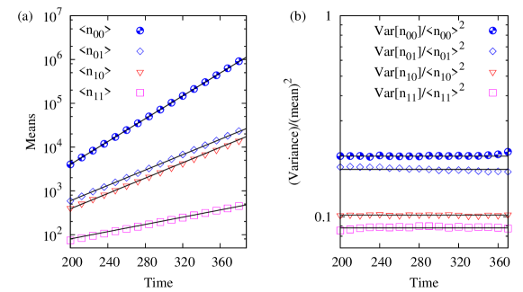
Figure 5: (a) Linear-log plot of $\langle n_{00}\rangle$, $\langle n_{01}\rangle$, $\langle n_{10}\rangle$ and $\langle n_{11}\rangle$ versus time $t$ for four-species HGT. Data from kinetic Monte-Carlo simulation are shown in various symbols as indicated. The fitted exponential functions (solid continuous straight lines) are: $\langle n_{00}\rangle\sim 10.0\times\exp(\lambda_{1}t)$; $\langle n_{01}\rangle\sim 10.5\times\exp(\lambda_{2}t)$; $\langle n_{10}\rangle\sim 8.6\times\exp(\lambda_{2}t)$ and $\langle n_{11}\rangle\sim 12.0\times\exp(\lambda_{4}t)$ (see Eq. (22) in Appendix C). (b) Linear-log plot of $Var[n_{00}]/\langle n_{00}\rangle^{2}$, $Var[n_{01}]/\langle n_{01}\rangle^{2}$, $Var[n_{10}]/\langle n_{10}\rangle^{2}$ and $Var[n_{11}]/\langle n_{11}\rangle^{2}$ versus time $t$ for four-species HGT. The straight lines show that the data are constant with time. The data are for $n_{00}(0)=n_{01}(0)=n_{10}(0)=n_{11}(0)=10$, $\beta_{1}=0.03$, $\beta_{2}=\beta_{3}=0.02$, $\beta_{4}=0.01$, $r=0.0005$, $q_{0}=0.9$ and $q_{1}=0.1$. The data are obtained by averaging over $10^{5}$ independent histories.

The reactions $R_{1}$ to $R_{4}$ are linear birth processes and the reactions $R_{5}$ to $R_{12}$ represent the nonlinear interactions through HGT. The rate of HGT in this model is $r$ and we will also assume that $\{\beta_{1},\beta_{2},\beta_{3},\beta_{4}\}>>r$. The Master equation is non-linear (in population sizes) in general. However at large times, the nonlinear terms may be approximated to linear ones for the choice of parameters: $n_{00}>>\{n_{01},n_{10},n_{11}\}$, $n_{00}>>n_{01}^{2}$, $\beta_{1}>\{\beta_{2},\beta_{3},\beta_{4}\}$, and $0<q_{i}<1/2$, $1/2<q_{1-i}<0$ (where $i=0$ or $1$). From the approximate linear Master equation we get the ODEs for the moments and solving them get the following solutions for the means:

$$\langle n_{00}\rangle \approx c_{1}e^{\lambda_{1}t}+c_{2}e^{\lambda_{2}t}+c_{3}e^{\lambda_{3}t}+c_{4}e^{\lambda_{4}t}$$

$$\langle n_{01}\rangle \approx k_{1}e^{\lambda_{2}t}+k_{2}e^{\lambda_{3}t}+k_{3}e^{\lambda_{4}t}$$

$$\langle n_{10}\rangle \approx k_{1}^{{}^{\prime}}e^{\lambda_{2}t}+k_{2}^{{}^{\prime}}e^{\lambda_{3}t}+k_{3}^{{}^{\prime}}e^{\lambda_{4}t}$$

$$\langle n_{11}\rangle \approx ke^{\lambda_{4}t},$$

where

$$\lambda_{1} = \beta_{1}~{}~{},~{}~{}\lambda_{2}=\left(\frac{\beta_{2}+\beta_{3}}{2}-\frac{r}{4}\right)+\sqrt{b}$$

$$\lambda_{3} = \left(\frac{\beta_{2}+\beta_{3}}{2}-\frac{r}{4}\right)-\sqrt{b}~{}~{},~{}~{}\lambda_{4}=\beta_{4}-r$$

$$b = r^{2}+4(\beta_{2}-\beta_{3}-r+2rq_{0})(\beta_{2}-\beta_{3}+2r(q_{0}-q_{1}))$$ (22)

Here $c_{1},\cdots,k$ are constants. Note that $\lambda_{2}>\lambda_{3}$ always, but nothing can be concluded about the relative magnitudes of $\lambda_{2}$ and $\lambda_{4}$, which will depend on the exact parameter values. Thus two cases can arise at large times: (i) for $\lambda_{2}>\lambda_{4}$, we have $\langle n_{00}\rangle\sim e^{\lambda_{1}t}$, $\langle n_{01}\rangle\sim\langle n_{10}\rangle\sim e^{\lambda_{2}t}$ and $\langle n_{11}\rangle\sim e^{\lambda_{4}t}$; while (ii) for $\lambda_{2}<\lambda_{4}$, we get $\langle n_{00}\rangle\sim e^{\lambda_{1}t}$ and $\langle n_{01}\rangle\sim\langle n_{10}\rangle\sim\langle n_{11}\rangle\sim e^{\lambda_{4}t}$.

We exactly simulate the reactions of Eq. (21) using kinetic Monte-Carlo. In certain regions of parameter space, at large times, we do find LD like behavior with the associated GNF property. We show the data for means and variances at large times in Fig. 5, for one such parameter and number regime defined by the following relations: (i) $\beta_{1}>\{\beta_{2},\beta_{3},\beta_{4}\}$, (ii) $0<q_{i}<1/2$ and $1/2<q_{1-i}<0$, where $i=0$ or $1$, (iii) $n_{00}>>\{n_{01},n_{10},n_{11}\}$, and (iv) $n_{00}>>n_{01}^{2}$. The GNF property holds for each species as is clearly evident from Fig. 5b. We also find a match between our data and the approximate analytical answer (Fig. 5a). We note that unlike the two-species HGT, for the four-species HGT the reduction to LD like behavior may not be true in general for all regions of the parameter space.

Similar analysis as above holds for two other parameter and number regimes : (1) $\beta_{4}>\{\beta_{1},\beta_{2},\beta_{3}\}$, $n_{11}>>\{n_{01},n_{10},n_{00}\}$ and $n_{00}>>n_{01}^{2}$; (2) $n_{11}\sim n_{01}\sim n_{10}\sim n_{00}$.

References

- Akiba et al. (1960) Akiba, T., Koyama, K., Ishiki, Y., Kimura, S., Fukushima, T., 1960. On the mechanism of the development of multiple-drug-resistant clones of shigella. Jpn J Microbiol 4, 219–227.
- Alberts et al. (2002) Alberts, B., Johnson, A., Lewis, J., Raff, M., Roberts, K., Walter, P., 2002. Molecular Biology of the cell. Garland Science–New York.
- Armitage (1952) Armitage, P., 1952. The statistical theory of bacterial populations subject to mutation. J. Royal Statist. Soc. B 14, 1–40.
- Babić et al. (2008) Babić, A., Lindner, A.B., Vulić, M., Stewart, E.J., Radman, M., 2008. Direct visualization of horizontal gene transfer. Science 319, 1533–1536.
- Barlow (2009) Barlow, M., 2009. What antimicrobial resistance has taught us about horizontal gene transfer. Methods Mol Biol 532, 397–411.
- Bertlett (1978) Bertlett, M.S., 1978. An introduction to stochastic processes. Cambridge, London.
- Bortz et al. (1975) Bortz, A.B., Kalos, M.H., Lebowitz, J.L., 1975. A new algorithm for Monte Carlo simulation of Ising spin systems. J. Comput. Phys. 17, 10–18.
- Bunting (1946) Bunting, I.M., 1946. The inheritance of color in bacteria, with special reference to Serratia marcescens. Cold Spring Harbor Symp. Quant. Biol. 11, 25–32.
- Chen et al. (2005) Chen, I., Christie, P.J., Dubnau, D., 2005. The ins and outs of DNA transfer in bacteria. Science 310, 1456–1460.
- Chia et al. (2008) Chia, N., Woese, C.R., Goldenfeld, N., 2008. A collective mechanism for phase variation in biofilms. Proc. Natl. Acad. Sci. USA 105, 14597–14602.
- Court et al. (2007) Court, D.L., Oppenheim, A.B., Adhya, S.L., 2007. A new look at bacteriophage genetic networks. J. Bacteriology 189, 298–304.
- Delbrück (1940) Delbrück, M., 1940. Statistical fluctuations in autocatalytic reactions. J. Chem. Phys. 8, 120–124.
- Gillespie (1976) Gillespie, D.T., 1976. A general method for numerically simulating the stochastic time evolution of coupled chemical reactions. J. Comput. Phys. 22, 403–434.
- Gillespie (2007) Gillespie, D.T., 2007. Stochastic simulation of chemical kinetics. Annu. Rev. Phys. Chem. 58, 35–55.
- Goldenfeld and Woese (2007) Goldenfeld, N., Woese, C., 2007. Biology’s next revolution. Nature 445, 369.
- Kourilsky (1973) Kourilsky, P., 1973. Lysogenization by bacteriophage Lamda. Molec. gen. Genet. 122, 183–195.
- Lea and Coulson (1949) Lea, D.E., Coulson, C.A., 1949. The distribution of the numbers of mutants in bacterial populations. J. Genetics 49, 264–285.
- Lieb (1951) Lieb, M., 1951. Forward and reverse mutation in a Histidine-requiring strain of Escherichia Coli. Genetics 86, 460–477.
- Luria and Delbrück (1943) Luria, S.E., Delbrück, M., 1943. Mutations of bacteria from virus sensitivity to virus resistence. Genetics 28, 491–511.
- Ma et al. (1992) Ma, W., Sandri, G., Sarkar, S., 1992. Analysis of the Luria-Delbrück distribution using discrete convolution powers. J. Appl. Prob. 29, 255–267.
- Mandelbort (1974) Mandelbort, B., 1974. A population birth-and-mutation process, i: explicit distributions for the number of mutants in an old culture of bacteria. J. Appl. Prob 11, 437–444.
- McCann et al. (1975) McCann, J., Choi, E., Yamasaki, E., Ames, B.N., 1975. Detection of carcinogens as mutagens in the salmonella/microsome test: assay of 300 chemicals. Proc Natl Acad Sci U S A 72, 5135–5139.
- Mortelmans and Zeiger (2000) Mortelmans, K., Zeiger, E., 2000. The ames salmonella/microsome mutagenicity assay. Mutat Res 455, 29–60.
- Ochman et al. (2000) Ochman, H., Lawrence, J.G., Groisman, E.A., 2000. Lateral gene transfer and the nature of bacterial innovation. Nature 405, 299–304.
- Qi Zheng (1999) Qi Zheng, 1999. Progress of a half century in the study of the Luria-Delbruck distribution. Math. Biosci. 162, 1–32.
- Rosche and Foster (2000) Rosche, W.A., Foster, P.L., 2000. Determining mutation rates in bacterial populations. Methods 20, 4–17.
- Sneppen and Zocchi (2005) Sneppen, K., Zocchi, G., 2005. Physics in molecular biology. Cambridge University Press.
- Tan and Piantadosi (1991) Tan, W.Y., Piantadosi, S., 1991. On stochastic growth processes with application to stochastic logistic growth. Satistica Sinica 1, 527–540.
- Wang and Goldenfeld (2010) Wang, Z., Goldenfeld, N., 2010. Fixed points and limit cycles in the population dynamics of lysogenic viruses and their hosts. Phys. Rev. E 82, 011918.
- Weitz and Dushoff (2008) Weitz, J.S., Dushoff, J., 2008. Alternative stable states in host-phage dynamics. Theor. Ecol. 1, 13–19.
- Weitz et al. (2008) Weitz, J.S., Mileyko, Y., Joh, R.I., Voit, E.O., 2008. Collective decision making in bacterial viruses. Biophys. J. 95, 2673–2680.
- Zeng et al. (2010) Zeng, L., Skinner, S.O., Zong, C., Sippy, J., Feiss, M., Golding, I., 2010. Decision making at a subcellular level determines the outcome of Bacteriophage infection. Cell 141, 682–691.
- Zhang et al. (2010) Zhang, H.P., Be er, A., Florin, E.L., Swinney, H.L., 2010. Collective motion and density fluctuations in bacterial colonies. Proc. Natl. Acad. Sci. USA 107, 13626–13630.
- Zhang et al. (2009) Zhang, H.P., Be er, A., Smith, R.S., Florin, E.L., Swinney, H.L., 2009. Swarming dynamics in bacterial colonies. Europhys. Lett. 87, 1–5.