Time-dependent quantum graph

Abstract

In this paper we study quantum star graphs with time-dependent bond lengths. Quantum dynamics is treated by solving Schrodinger equation with time-dependent boundary conditions given on graphs. Time-dependence of the average kinetic energy is analyzed. Space-time evolution of the Gaussian wave packet is treated for harmonically breathing star graph.

Quantum particle dynamics in nanoscale networks and discrete structures is of fundamental and practical importance. Usually such systems are modeled by so-called quantum graphs, systems attracting much attention in physics Uzy1 -Uzy3 and mathematics Exner1 -Exner3 during past two decades.

In physics quantum graphs were introduced as a toy model for studies of quantum chaos by Kottos and Smilansky Uzy1 . However, the idea for studying of a system confined to a graph dates back to Pauling Pauling who suggested to use such systems for modeling free electron motion in organic molecules. During last two decades quantum graphs found numerous applications in modeling different discrete structures and networks in nanoscale and mesoscopic physics(e.g., see reviews Uzy1 -Uzy3 and references therein).

Mathematical properties of the Schrodinger operators on graphs Exner1 ; Exner2 ; Exner3 inverse problems for quantum graphs Kurasov ; Cheon were also subject for extensive research recently. Also, an experimental realization of quantum graphs was discussed earlier in the Ref. Hul . Despite the certain progress made in the study of quantum graphs some of important aspects are still remaining as less- or not explored. Especially, this concerns the problems of driven graphs, i.e. graphs perturbed by time-dependent external forces. An important example of such a driving force is that caused by driven (moving) boundaries. Treatment of such system can be reduced to the Schrödinger equation with time-dependent boundary conditions. Earlier, the problem of time-dependent boundary conditions has attracted much attention in the context of quantum Fermi acceleration jose -seb90 , though different aspects of the problem was treated by many authors mun81 -glas08 . Detailed study of the problem can be found in series of papers by Makowski and co-authors mak91 -mak923 . It was pointed out in the above Refs. that the problem of 1D box with the moving wall can be mapped onto that of time-dependent harmonic oscillator confined inside the static box mak91 .

In this paper we treat similar problem for quantum star graph, i.e. we study the problem of quantum graphs with time-dependent bonds. In particular, we consider harmonically breathing quantum star graphs, the cases of contracting and expanding graphs. The latter can be solved exactly analytically. Motivation for the study of time-dependent graphs comes from such practically important problems as quantum Fermi acceleration in nanoscale network structures, tunable particle transport in quantum wire networks, molecular wires, different lattices and discrete structures. In particular, sites, vertices, nodes of such discrete structures can fluctuate that makes them time-dependent. We will study time-dependence of the average kinetic energy and wave packet dynamics in harmonically breathing graphs.

Graphs are the systems consisting of bonds which are connected at the vertices. The bonds are connected according to a rule which is called topology of a graph. Topology of a graph is given by in terms of so-called adjacency matrix Uzy1 ; Uzy2 :

$$C_{ij}=C_{ji}=\left\{\begin{array}[]{c}1\qquad$if$\;i\;and\;j\;$are connected$\\ 0\qquad$ otherwise$\end{array}\right.i,j=1,2,...,V.$$

Quantum dynamics of a particle in a graph is described in terms of one-dimensional Schrödinger equation Uzy1 ; Uzy2 (in the units $\hbar=2m=1$):

$$-i\frac{d^{2}\Psi_{b}(x)}{dx^{2}}=k^{2}\Psi_{b}(x),\quad b=(i,j),$$ (1)

where $b$denotes a bond connecting $i$th and $j$the vertices, and for each bond $b$, the component $\Psi_{b}$ of the total wavefunction $\Psi_{b}$ is a solution of the eq.(1).

The wavefunction, $\Psi_{b}$, satisfies boundary conditions at the vertices, which ensure continuity and current conservation Uzy1 . General scheme for finding of eigenfunctions and eigenvalues for such boundary conditions can be found in the Ref.Uzy1 . Different types of boundary conditions for the Schrodinger equation on graphs are discussed in the Refs.Exner1 ; Exner2 ; Exner3 . In the following we restrict our consideration by most simplest graph, so-called star graph. The star graph consist of three or more bonds connected at the single vertex which is called branching point (see Fig.1). Other ones are called edge vertices. The eigenvalue problem for a star graph with $N$ bonds is given by the following Schrödinger equation:

$$-\frac{d^{2}}{dx^{2}}\phi_{j}(y)=k^{2}\phi_{j}(y),\ \ 0\leq y\leq l_{j},\ j=1,...,N.$$

Here we consider the following boundary conditions Keating :

$$\left\{\begin{array}[]{l}\phi_{1}|_{y=0}=\phi_{2}|_{y=0}=...=\phi_{N}|_{y=0},\\ \phi_{1}|_{y=l_{1}}=\phi_{2}|_{y=l_{2}}=...=\phi_{N}|_{y=l_{N}}=0,\\ \sum\limits_{j=1}^{N}{\frac{\partial}{\partial y}\phi_{j}|_{y=0}}=0.\\ \end{array}\right.$$ (2)

The eigenvalues can be found by solving the following equation Keating

$$\sum\limits^{N}_{j=1}{ctan(k_{n}l_{j})}=0$$

where corresponding eigenfunctions are given as Keating

$$\phi_{j}^{(n)}=\frac{B_{n}}{sin(k_{n}l_{j})}sin(k_{n}(l_{j}-y))$$

$$B_{n}=\sqrt{\frac{2}{\sum_{j}{\frac{l_{j}+sin(2k_{n}l_{j})}{sin^{2}(k_{n}l_{j})}}}}.$$

Time-dependent graph implies that lengths of the bonds of a graph are time-varying, i.e., when $L_{j}$ is a function of time. In this case particle dynamics in graph is described by the following time-dependent Schrödinger equation:

$$i\frac{\partial}{\partial t}\Psi_{j}(x,t)=-\frac{\partial^{2}}{\partial x^{2}}\Psi_{j}(x,t),\ \ 0<x<L_{j}(t),\ j=1,...,N,$$ (3)

with $N$ being the number of bonds.

In the following we will consider the boundary conditions given by

$$\left\{\begin{array}[]{l}\Psi_{1}|_{x=0}=\Psi_{2}|_{x=0}=...=\Psi_{N}|_{x=0},\\ \Psi_{1}|_{x=L_{1}(t)}=\Psi_{2}|_{x=L_{2}(t)}=...=\Psi_{N}|_{x=L_{N}(t)}=0,\\ \sum\limits_{j=1}^{N}{\frac{\partial}{\partial x}\Psi_{j}|_{x=+0}}=0.\\ \end{array}\right.$$

These boundary conditions imply that only edge vertices of the graph are moving while center (branching point) is fixed. Furthermore, we assume that $L_{j}(t)$ is given as $L_{j}(t)=l_{j}L(t)$, where $L(t)$ is a continuous function and $l_{j}$ are the positive constants. Then using the coordinate transformation

$$y=\frac{x}{L(t)},$$

Eq. (3) can be rewritten as

$$i\frac{\partial}{\partial t}\Psi_{j}(y,t)=-\frac{1}{L^{2}}\frac{\partial^{2}}{\partial y^{2}}\Psi_{j}(y,t)+i\frac{\dot{L}}{L}y\frac{\partial}{\partial y}\Psi_{j}(y,t),\ \ 0<y<l_{j},\ j=1,...,N.$$ (4)

It is clear that the Schrödinger operator in the right hand side of Eq. (4) is not Hermitian due to the presence of second term. Therefore using the transformation

$$\Psi_{j}(y,t)=\frac{1}{\sqrt{L}}e^{i\frac{L\dot{L}}{4}y^{2}}\varphi_{j}(y,t),$$

we can make it Hermitian as

$$i\frac{\partial}{\partial t}\varphi_{j}(y,t)=-\frac{1}{L^{2}}\frac{\partial^{2}}{\partial y^{2}}\varphi_{j}(y,t)+\frac{L\ddot{L}}{4}y^{2}\varphi_{j}(y,t),\ \ 0<y<l_{j},\ j=1,...,N.$$ (5)

We note that the above transformations of the wave function remain the boundary conditions unchanged.

Time and coordinate variables in Eq. (5) can be separated only in case when $L(t)$ obeys the equation

$$\frac{L^{3}\ddot{L}}{4}=-C^{2}=const,$$ (6)

In this case using the substitution $\varphi_{j}(y,t)=\phi_{j}(y)\cdot exp\left(-ik^{2}\int\limits_{0}^{t}\frac{ds}{L^{2}(s)}\right)$, we get

$$\frac{d^{2}\phi_{j}}{dy^{2}}+(\lambda-C^{2}y^{2})\phi_{j}=0,\ \ y\in(0,l_{j}).$$ (7)

For $C\not=0$ from Eq. (6) we have

$$L(t)=\sqrt{\alpha t^{2}+\beta t+\gamma},\ \ C^{2}=\frac{1}{16}(\beta^{2}-4\alpha\gamma),$$ (8)

and

$$L(t)=\sqrt{\beta t+\gamma},\ \ C^{2}=\frac{1}{16}\beta^{2}.$$ (9)

In both cases exact solutions of Eq.(5) can be obtained in terms confluent hypergeometric functions. In particular, for the case when time-dependence of $L(t)$ is given by Eq.(9) fundamental solutions of Eq.(5) can be written as

$$\phi_{j,1}=y\exp\left(\frac{C}{2}y\right)M\left(\frac{3}{4}-\frac{k}{4C},\frac{3}{2},-Cy^{2}\right),$$

and

$$\phi_{j,1}=\exp\left(\frac{C}{2}y\right)M\left(\frac{1}{4}-\frac{k}{4C},\frac{1}{2},-Cy^{2}\right).$$

Therefore the general solution of Eq.(5) is given as

$$\phi_{j}(y)=A_{j}\phi_{j,1}+B_{j}\phi_{j,2}.$$ (10)

From the boundary conditions given by Eq.(2) we have

$$B_{j}=A,\ \ A_{j}=A\cdot\alpha_{j}(k),\ \ j=1,2,3,...,N,$$

where $B$ is an arbitrary constant and

$$\alpha_{j}(k)=-\frac{M\left(\frac{1}{4}-\frac{k}{4C},\frac{1}{2},-Cl_{j}^{2}\right)}{l_{j}M\left(\frac{3}{4}-\frac{k}{4C},\frac{3}{2},-Cl_{j}^{2}\right)},\ \ j=1,2,...,N.$$

Taking to account the relations $\left.\frac{d\phi_{j,1}(y)}{dy}\right|_{y=0}=1$, $\left.\frac{d\phi_{j,2}(y)}{dy}\right|_{y=0}=\frac{C}{2},$ from Eq. (2) we obtain the following spectral equation for finding the eigenvalues, $k_{n}$ of Eq.(5):

$$\sum_{j=1}^{N}\frac{1}{l_{j}}\frac{M\left(\frac{1}{4}-\frac{k}{4C},\frac{1}{2},-Cl_{j}^{2}\right)}{M\left(\frac{3}{4}-\frac{k}{4C},\frac{3}{2},-Cl_{j}^{2}\right)}=\frac{CN}{2}.$$ (11)

(a)                                    (b)

(c)

Figure 1: Time-dependence of the average kinetic energy for harmonically oscillating primary star graph.

Thus the eigenfunctions of Eq.(5) can be written as

$$\phi_{j}(y,k_{n})=A\left[\alpha_{j}(k_{n})\phi_{j,1}(y)+\phi_{j,2}(y)\right],\ \ j=1,2,...,N.$$ (12)

Furthermore, we provide the solution of Eq.(5) for simplest case $L(t)=at+b$, which correspond to $C=0$ in Eq.(6). In this case of the eigenvalues of Eq.(5) can be written as time-dependence of the wall is given as

$$\phi_{j}(y,k_{n})=\frac{A}{sin(\sqrt{k_{n}}l_{j})}sin(\sqrt{k_{n}}(l_{j}-y)),\ \ j=1,2,...,N,$$ (13)

where $k_{n}$ is the $n$th positive root of the equation

$$\sum_{j=1}^{N}ctan(l_{j}^{2}\sqrt{k})=0.$$ (14)

and $L(t)>0$, $B$ is the normalization constant.

Now let us consider harmonically breathing graph, i.e. the case when time-dependence of $L(t)$ is given as

$$L(t)=b+a\cos\omega t$$

with $\omega=\frac{2\pi}{T}$ being oscillation frequency and T is the oscillation period. It is clear that in this case time and coordinate variables in Eq. (5) cannot be separated. Expanding $\varphi(y,t)$ in Eq. (5) in terms of static graphs wave functions as

$$\varphi_{j}(y,t)=\sum\limits_{n}{C_{n}(t)\phi_{j}^{(n)}(y)},$$ (15)

and inserting this expansion into Eq.(5)we have

$$\dot{C}_{n}(t)=\sum\limits_{m}{M_{mn}C_{m}(t)}$$

where

$$M_{mn}=-i\frac{k^{2}_{m}}{L^{2}(t)}-i\frac{L\ddot{L}}{4}K_{mn}$$

The quantity we are interested to compute is the average kinetic energy which is defined as

$$E(t)=\langle\psi|H|\psi\rangle=\sum_{j=1}^{N}\int\limits_{0}^{L_{j}(t)}\left|\frac{\partial\psi_{j}(x,t)}{\partial x}\right|^{2}dx.$$ (16)

In Fig. 1 time dependence of the average kinetic energy of the harmonically breathing star graph is presented for different values of the breathing frequency and amplitude. As it can be seen from these plots, $<E(t)>$ is almost periodic for $\omega=0.5$ and $a=1$, while for $\omega=10$ and $a=1$ such a periodicity is completely broken and energy grows in time. For $\omega=10$ and $a=20$ the behavior of $<E(t)>$ demonstrates ”quasiperiodic behavior”. Appearing of periodic behavior in $<E(t)>$ can be explained by synchronization of the motion of particle with the frequency. The lack of such synchronization causes breaking of the periodicity of the average energy in time.

Furthermore, we consider wave packet evolution in harmonically breathing star graph by taking the wave function at $t=0$ (for the first bond) as the following Gaussian wave packet:

$$\Psi_{1}(x,0)=\Phi(x)=\frac{1}{\sqrt{2\pi}\sigma}e^{-\frac{(x-\mu)^{2}}{2\sigma}},$$ (17)

with $\sigma$ being the width of the packet. For other bonds initial wave function is assumed to be zero, i.e. $\Psi_{2}(x,0)=\Psi_{3}(x,0)=0$. Then for the initial values of the functions $\varphi^{(j)}(y,t)$ in Eq. (15) we have

$$\varphi^{(j)}(y,0)=L(0)e^{-i\frac{L(0)\dot{L}(0)}{4}y^{2}}\Phi(y).$$

Correspondingly, the expansion coefficients at $t=0$ can be written as

$$C_{n}(0)=\sum_{j}\int_{0}^{l_{j}}\varphi^{(j)}(y,0)\phi_{n}^{(j)}(y)^{*}.$$

In calculation of the wave packet evolution we will choose initial condition as the wave packet being on the first bond only, while for other two bonds the wave function at $t=0$ is taken as zero. In Fig.2 the time evolution of the wave packet is plotted for harmonically breathing primary star graph whose bonds oscillate according to the law $L(t)=40+a\cos\omega t$ . The oscillation parameters (frequency and amplitude) are chosen as follows: a) $\omega=10,$  $a=20;$ b) $\omega=10,$  $a=1;$  c) $\omega=0.5,$  $a=1.$ Fig.2d presents wave packet evolution in static(time-independent) star graph. At $t=0$ a Gaussian packet of the width $\sigma$ and velocity $v_{0}$ is assumed being in the first bond. As it can be seen from these plots, for higher frequencies dispersion of the packet and its transition to other bonds occur more faster compared to that for smaller smaller frequencies. Again, an important role plays here possible synchronization between the bond edge and wave packets motions. Existence or absence of ssuch synchronization defines how the collision of the packet with the bond edges will occur and how extensively it gains or loses its energy. Therefore more detailed treatment of the wave packet dynamics in harmonically breathing graphs should be based on the analysis of the role of synchronization and its criterions.

In this paper we have treated time-dependent quantum network by considering expanding and harmonically breathing quantum star graphs. Edge boundaries are considered to be time-dependent, while branching point is assumed to be fixed(static). Time-dependence of the average kinetic energy and space-time evolution of the Gaussian wave packet are studied by solving the Schrodinger equation with time-dependent boundary conditions. It is shown that for certain frequencies energy is a periodic function of time, while for others it gan be non-monotonically growing function of time. Such a feature can be caused by possible synchronization of of the particles motion and the motions of the moving edges of graph bonds. Similar feature can be seen also from the analysis of the wave packet evolution. The above study can be useful for the treatment of particle transport in different discrete structures, such as molecular and quantum wire networks, networks of carbon nanotubes, crystal lattices, and others nanoscale systems that can be modeled by quantum graphs.

(a)                                    (b)

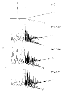
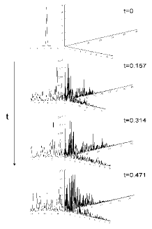
(c)                                    (d)

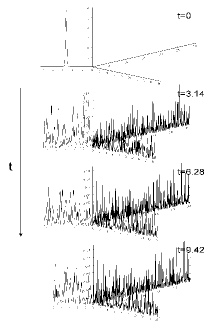
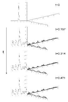
Figure 2: Time evolution of the Gaussian wave packet given by Eq. (17) for the parameters: a) $\omega=10,$  $a=20;$ b) $\omega=10,$  $a=1;$  c) $\omega=0.5,$  $a=1;$  d) Wave packet evolution in static star graph.

References

- (1) Tsampikos Kottos and Uzy Smilansky, Ann.Phys., 76 274 (1999).
- (2) Sven Gnutzmann and Uzy Smilansky, Adv.Phys. 55 527 (2006).
- (3) S. GnutzmannJ.P. Keating b, F. Piotet, Ann.Phys., 325 2595 (2010).
- (4) L. Pauling, J. Chem. Phys. 4 673 (1936).
- (5) P.Exner, P.Seba, P.Stovicek, J. Phys. A: Math. Gen. 21 4009-4019 (1988).
- (6) P.Exner, P.Seba, Rep. Math. Phys., 28 7 (1989).
- (7) P.Exner, Ann. Inst. H. Poincare: Phys. Theor, 66 359 (1997).
- (8) J. Boman, P. Kurasov, Adv. Appl. Math., 35, 58 (2005)
- (9) , T. Cheon, P. Exner, O. Turek, Ann.Phys., 325 548 (2010).
- (10) Oleh Hul et al, Phys. Rev. E 69, 056205 (2004).
- (11) J.P.Keating, Contemp. Math., 415, 191 (2006).
- (12) J.V. Jose, R. Gordery Phys. Rev. Lett. 56, 290 (1986).
- (13) G. Karner, Lett. Math. Phys. A 17, 329 (1989).
- (14) P. Seba. Phys. Rev. A 41, 2306 (1990).
- (15) S.W. Doescher and M.H. Rice Am. J. Phys. 37, 1246 (1969).
- (16) A. Munier, J.R. Burgan, M. Feix and E. Fijalkow. J. Math. Phys. 22, 1219 (1981).
- (17) D.N. Pinder, Am. J. Phys. 58, 54 (1990).
- (18) M. Razavy. Phys. Rev. A 44, 2384 (1991).
- (19) P. Pereshogin, P. Pronin, Phys. Lett. A 156, 12 (1991).
- (20) C. Scheininger and M. Kleber. Physica D 50, 391 (1991).
- (21) A.J. Makowski and S.T. Dembinski. Phys. Lett. A 154, 217 (1991).
- (22) A.J. Makowski and P. Peplowski. Phys. Lett. A 163, 142 (1992).
- (23) A.J. Makowski. J. Phys. A: Math. Gen. 25, 3419(1992).
- (24) J.E. Willemsen, Phys. Rev. E 50, 3116 (1994).
- (25) D.A. Moralez, Z. Parra, R. Almeida, Phys. Lett. A 185, 273 (1994).
- (26) C. Yuce, Phys. Lett. A 321, 291 (2004).
- (27) M.L. Glasser, J. Mateo, J. Negro and L.M. Nieto, Chaos, Solitons and Fractals, 41, 2067 (2009).