Efficient Computing Budget Allocation for Simulation-based Optimization with Stochastic Simulation Time

Abstract

The dynamics of many systems nowadays follow not only physical laws but also man-made rules. These systems are known as discrete event dynamic systems and their performances can be accurately evaluated only through simulations. Existing studies on simulation-based optimization (SBO) usually assume deterministic simulation time for each replication. However, in many applications such as evacuation, smoke detection, and territory exploration, the simulation time is stochastic due to the randomness in the system behavior. We consider the computing budget allocation for SBO’s with stochastic simulation time in this paper, which has not been addressed in existing literatures to the author’s best knowledge. We make the following major contribution. The relationship between simulation time and performance estimation accuracy is quantified. It is shown that when the asymptotic performance is of interest only the mean value of individual simulation time matters. Then based on the existing optimal computing budget allocation (OCBA) method for deterministic simulation time we develop OCBA for stochastic simulation time (OCBAS), and show that OCBAS is asymptotically optimal. Numerical experiments are used to discuss the impact of the variance of simulation time, the impact of correlated simulation time and performance estimation, and to demonstrate the performance of OCBAS on a smoke detection problem in wireless sensor network. The numerical results also show that OCBA for deterministic simulation time is robust even when the simulation time is stochastic.

Index Terms— Discrete event dynamic system, simulation-based optimization, optimal computing budget allocation.

I Introduction

The dynamics of many systems nowadays follow not only physical laws but also man-made rules. These systems are known as discrete event dynamic systems (DEDS’s). Simulation is usually the only faithful way to accurately describe the dynamics of such systems. The performance optimization of these systems then enter the realm of simulation-based optimization (SBO). Most existing studies on SBO assume deterministic simulation time for each replications. However, there exist a large set of DEDS’s where the simulation time is stochastic. Estimating the evacuation time for a building, the smoke detection time of a wireless sensor network, and the exploration time of a multi-agent system under a collaborative search policy are such examples. It is of great practical interest to allocate the computing budget among designs so that the best design can be found with high probability. However, to the author’s best knowledge, this problem has not been considered in existing literatures.

We consider this important problem in this paper. Simulation-based optimization with stochastic simulation time is nontrivial due to the following difficulties. First, simulation-based performance evaluation. Simulation is usually time-consuming, and only provides noisy estimations. In order to obtain an accurate performance estimation, one has to run simulation by infinite times, which is infeasible in practice. Second, discrete variables. Designs usually take discrete and finite values. This not only makes traditional gradient-based search algorithms not applicable, but also makes the size of the search space increase exponentially fast when the system scale increases, which is also known as the curse of dimensionality. Third, the huge number of computing budget allocations. One usually does not have time to explore all the allocations to find the optimum. Instead, sequential allocations that can iteratively improve their performances are of more practical interest. Fourth, stochastic simulation time. Giving the total simulation time that is allocated to a design, it is not clear how many replications can be finished. Thus the resulting performance estimation accuracy is not clear.

There exist abundant literatures to address the above first three difficulties. For example, ranking and selection (R&S) procedures are typical procedures for SBO. Bechhofer et al.[1], Swisher et al.[2], and Kim and Nelson[3] provided excellent review of the R&S works. Chen[4], Chen et al.[5], Chen et al.[6], and Chen and Yücesan[7] developed the optimal computing budget allocation (OCBA) procedure to maximize the probability of correctly selecting the best design under a given computing budget. OCBA has been shown to perform asymptotically optimally when the simulation time is (identically or nonidentically) deterministic. OCBA has been extended to tackle the case where the deterministic computing time for one simulation replication is different across the alternatives[8], to handle multiple objective functions[9, 10], simulation-based constraints[11], opportunity cost[12], and complexity preferences[13]. A comprehensive introduction to OCBA is recently available in [14]. Recent good surveys on other methods for SBO can be found in [15, 16, 17, 18, 19]. The above existing literatures assume deterministic simulation time and do not address the aforementioned difficulty of stochastic simulation time.

In this paper we consider the computing budget allocation for SBO with stochastic simulation time and make the following major contribution. The relationship between the total simulation time and the accuracy of performance estimation is quantified. It is shown that when the asymptotic performance is of interest only the mean value of individual simulation time matters. Then based on OCBA for deterministic simulation time we develop OCBA for stochastic simulation time (OCBAS) and show that OCBAS is asymptotically optimal. Numerical experiments are used to discuss the impact of the variance of simulation time, the impact of correlated simulation time and performance estimation, and to demonstrate the performance of OCBAS on a smoke detection problem in wireless sensor network. The numerical results also show that OCBA for deterministic simulation time is robust even when the simulation time is stochastic.

The rest of this paper is organized as follows. We present the mathematical problem formulation in section II, provide the main results in section III, show the numerical results in section IV, and briefly conclude in section V.

II Problem Formulation

Consider a finite set of designs $\Theta=\{1,\ldots,k\}$. Let $J_{i}$ be the true performance of design $i$, which can be accurately evaluated only through infinite number of replications

$$J_{i}=\lim_{n\rightarrow\infty}\frac{1}{n}\sum_{j=1}^{n}\hat{J}_{i}(\xi_{j}),$$

where $n$ is the number of replications that are used,

$$\hat{J}_{i}(\xi_{j})=J_{i}+w_{i}(\xi_{j}),$$

$\xi_{j}$ represents the randomness in the $j$-th sample path, and $w_{i}$ has i.i.d. Gaussian distribution $N(0,\sigma_{i}^{2})$. Let $t_{i}$ denote the time that is consumed by an individual replication of design $i$. We assume the simulation is conducted by a digital computer and thus $t_{i}$ takes positive integer values and is stochastic. Let $f_{i}$ and $F_{i}$ be the probability density function (PDF) and cumulative distribution function (CDF) of $t_{i}$, respectively. Assume that $\hat{J}_{i}$ and $t_{i}$ are mutually independent. The case when $\hat{J}_{i}$ and $t_{i}$ are correlated will be discussed in section IV.

Giving $T_{i}$, the number of replications that design $i$ can be simulated is stochastic, which is denoted as $n_{i}$. Then we have

$$\sum_{j=1}^{n_{i}}t_{i,j}\leq T_{i}<\sum_{j=1}^{n_{i}+1}t_{i,j},$$

where $t_{i,j}$ is the simulation time for the $j$-th simulation of design $i$. Assume that an incomplete simulation does not output any estimate. When $T_{i}$ is large, it is reasonable to assume that $n_{i}>0$. The estimate of $J_{i}$ is

$$\bar{J}_{i}=\frac{1}{n_{i}}\sum_{j=1}^{n_{i}}\hat{J}_{i}(\xi_{j}).$$

We take the Bayesian viewpoint, which means that the estimates $\bar{J}_{1},\ldots,\bar{J}_{k}$ are given and the true performances $J_{1},\ldots,J_{k}$ have posterior estimates $\tilde{J}_{1},\ldots,\tilde{J}_{k}$. Let $g_{i}$ and $G_{i}$ be the PDF and CDF of $\tilde{J}_{i}$, respectively. Sort the designs from small to large according to $\bar{J}_{i}$, and denote the best design as $b$. Define the probability of correct selection (PCS) as

$$PCS=\Pr\left\{\tilde{J}_{b}\leq\tilde{J}_{i},i=1,\ldots,k\text{ and }i\neq b\right\}.$$

In other words, we are interested in the probability that the observed best is the truly best. Now we can mathematically formulate the problem as

$$\max_{T_{1},\ldots,T_{k}}PCS\text{ s.t. }\sum_{i=1}^{k}T_{i}=T,$$

where $T$ is the total computing budget. In the following discussion we will refer this problem as P1. In other words, we are looking for an allocation of the simulation time among the designs so that the probability of correct selection is maximized. Note that regarding $t_{i,j}$ as the event occurrence time and $\hat{J}_{i}(\xi_{j})$ as the reward, then $\{n_{i}(T_{i})\bar{J}_{i}(T_{i})\}$ is a renewal reward process[20]. This fact will be used to show that $G_{i}$ can be approximated by a Gaussian (Lemma 3).

III Main Results

In this section, we address problem P1 in three steps. First, the relationship between the simulation time $T_{i}$ and the distribution of $\tilde{J}_{i}$ is quantified. Second, an approximation of the PCS is provided. Then an approximate version of problem P1 is formulated and denoted as problem P2. Third, OCBAS is developed and is shown to solve P2 asymptotically optimally.

We start from quantifying the distribution of $n_{i}$.

Lemma 1

For any nonnegative integer $c$, we have

$$\Pr\left\{n_{i}\geq c\right\}=\left\{\begin{array}[]{ll}(F_{i}*f_{i}^{c-1})(T_{i}),&c\geq 1,\\ 1,&c=0,\end{array}\right.$$

where $[f*g](t)$ represents the convolution of $f$ and $g$, i.e.,

$$[f*g](t) \equiv \int_{-\infty}^{\infty}f(\tau)g(t-\tau)d\tau;$$

$$f^{a} \equiv \underbrace{f*\cdots*f}_{a},$$

and $f^{0}$ is the Dirac delta function.

Proof:

When $c=0$, we have $\Pr\left\{n_{i}\geq 0\right\}=1$. When $c\geq 1$, we have $\Pr\left\{n_{i}\geq c\right\}=\Pr\left\{\sum_{j=1}^{c}t_{i,j}\leq T_{i}\right\}$. Then we prove by induction.
Step 1. $c=1$. We have $\Pr\left\{n_{i}\geq 1\right\}=\Pr\left\{t_{i,1}\leq T_{i}\right\}=F_{i}(T_{i})=(F_{i}*f^{0})(T_{i})$.
Step 2. Suppose that we have

$$\Pr\left\{n_{i}\geq c\right\}=\Pr\left\{\sum_{j=1}^{c}t_{i,j}\leq T_{i}\right\}=(F_{i}*f^{c-1})(T_{i}).$$

Step 1 has provided one such example for $c=1$. We have

$$\Pr\left\{n_{i}\geq c+1\right\}=\Pr\left\{\sum_{j=1}^{c+1}t_{i,j}\leq T_{i}\right\}$$

$$= \int\Pr\left\{\sum_{j=1}^{c}t_{i,j}+t_{i,c+1}\leq T_{i}\Bigg{|}\sum_{j=1}^{c}t_{i,j}=x\right\}$$

$$\times\Pr\left\{\sum_{j=1}^{c}t_{i,j}=x\right\}dx$$

$$= \int\Pr\left\{t_{i,c+1}\leq T_{i}-x\right\}d\Pr\left\{\sum_{j=1}^{c}t_{i,j}\leq x\right\}$$

$$= \int F_{i}(T_{i}-x)d(F_{i}*f_{i}^{c-1})(x)$$

$$= \int F_{i}(T_{i}-x)f_{i}^{c}(x)dx=(F_{i}*f_{i}^{c})(T_{i}).$$

Combining steps 1 and 2 together, we have

$$\Pr\left\{n_{i}\geq c\right\}=(F_{i}*f_{i}^{c-1})(T_{i}).$$

This completes the proof. ∎

Lemma 2

$$\Pr\left\{n_{i}=c\right\}=\left\{\begin{array}[]{ll}\left[F_{i}*(f_{i}^{c-1}-f_{i}^{c})\right](T_{i}),&c\geq 1,\\ 1-F_{i}(T_{i}),&c=0.\end{array}\right.$$

Proof:

When $c=0$, we have

$$\Pr\left\{n_{i}=0\right\}=\Pr\left\{t_{i,1}>T_{i}\right\}=1-F_{i}(T_{i}).$$

When $c\geq 1$, we have

$$\Pr\left\{n_{i}=c\right\} = \Pr\left\{n_{i}\geq c\right\}-\Pr\left\{n_{i}\geq c+1\right\}$$

$$= (F_{i}*f_{i}^{c-1})(T_{i})-(F_{i}*f_{i}^{c})(T_{i})$$

$$= \left[F_{i}*(f_{i}^{c-1}-f_{i}^{c})\right](T_{i}).$$

This completes the proof. ∎

Now we have

Theorem 1

$G_{i}(x)=\sum_{c=1}^{\infty}\Phi\left(\frac{x-\bar{J}_{i}}{\sigma_{i}/\sqrt{c}}\right)\left[F_{i}*(f_{i}^{c-1}-f_{i}^{c})\right](T_{i})$ $+G_{i}^{0}(x)\left[1-F_{i}(T_{i})\right]$, where $\Phi(\cdot)$ is the CDF of $N(0,1)$ and $G_{i}^{0}(x)$ is the a priori CDF of $J_{i}$.

Proof:

We have

$$G_{i}(x)=\Pr\left\{\tilde{J}_{i}\leq x\right\}$$ (1)

$$= \sum_{c=1}^{\infty}\Pr\left\{\tilde{J}_{i}\leq x,n_{i}=c\right\}+G_{i}^{0}(x)\Pr\left\{n_{i}=0\right\}$$

$$= \sum_{c=1}^{\infty}\Pr\left\{\tilde{J}_{i}\leq x|n_{i}=c\right\}\Pr\left\{n_{i}=c\right\}+G_{i}^{0}(x)\Pr\left\{n_{i}=0\right\}.$$

Note that

$$\Pr\left\{\tilde{J}_{i}\leq x|n_{i}=c\right\}=\Pr\left\{\sum_{j=1}^{c}\hat{J}_{i}(\xi_{j})/c\leq x\right\}=\Phi\left(\frac{x-\bar{J}_{i}}{\sigma_{i}/\sqrt{c}}\right),$$ (2)

where the first equality follows from the assumption that $\hat{J}_{i}$ and $t_{i}$ are independent, and the second equality follows from the assumption that $\hat{J}_{i}(\xi_{j})$ are i.i.d. Gaussian. Combine Eqs. (1) and (2) and Lemma 2, we then have

$$G_{i}(x)=\sum_{c=1}^{\infty}\Phi\left(\frac{x-\bar{J}_{i}}{\sigma_{i}/\sqrt{c}}\right)\left[F_{i}*(f_{i}^{c-1}-f_{i}^{c})\right](T_{i})+G_{i}^{0}(x)\left[1-F_{i}(T_{i})\right].$$

This completes the proof. ∎

Theorem 1 implies that $\tilde{J}_{i}$ is not Gaussian. Instead, its CDF $G_{i}(x)$ is a weighted average of a sequence of Gaussian CDF’s $\Phi\left(\frac{x-\bar{J}_{i}}{\sigma_{i}/\sqrt{c}}\right)$’s, which has equal mean values and decreasing variances. Note that when $T_{i}\rightarrow\infty$, $\Pr\{n_{i}=c\}$ is almost zero for most values of $c$ except for $c\approx T_{i}/\mu_{i}$, where $\mu_{i}=\mathbf{E}[t_{i}]$. In this case $c$ is the expected value of $n_{i}$. We have

Lemma 3

$\lim_{T_{i}\rightarrow\infty}\left(\sqrt{n_{i}}\left(\tilde{J}_{i}-\bar{J}_{i}\right)\leq x\right)=\Phi\left(x/\sigma_{i}\right).$

Proof:

Following the elementary renewal theorem[20], we have $\lim_{T_{i}\rightarrow\infty}{\mathbf{E}[n_{i}]}/{T_{i}}={1}/{\mu_{i}}.$ Thus when $T_{i}\rightarrow\infty$, $n_{i}$ also goes to infinity. Then Lemma 3 follows naturally from the central limit theorem. ∎

Lemma 3 implies that when $T_{i}$ is large, $G_{i}(x)$ can be reasonably approximated by $N(\bar{J}_{i},\sigma_{i}^{2}\mu_{i}/T_{i})$. The performance of the allocation procedure using this approximation will be shown by numerical experiments in section IV. Following the Bonferroni inequality we have

$$\Pr\left\{\tilde{J}_{b}\leq\tilde{J}_{i},i=1,\ldots,k\text{ and }i\neq b\right\}\geq 1-\sum_{i=1,i\neq b}^{k}\Pr\left\{\tilde{J}_{b}>\tilde{J}_{i}\right\}.$$

Following the above analysis $G_{b}(x)$ and $G_{i}(x)$ can be approximated by $\Phi\left(\frac{x-\bar{J}_{b}}{\sqrt{\sigma_{b}^{2}\mu_{b}/T_{b}}}\right)$ and $\Phi\left(\frac{x-\bar{J}_{i}}{\sqrt{\sigma_{i}^{2}\mu_{i}/T_{i}}}\right)$, respectively. Then we have

$$\Pr\left\{\tilde{J}_{b}>\tilde{J}_{i}\right\}\approx\int_{-\frac{\delta_{b,i}}{\sigma_{b,i}}}^{\infty}\frac{1}{\sqrt{2\pi}}\exp\left\{-\frac{t^{2}}{2}\right\}dt,$$

where $\delta_{b,i}=\bar{J}_{b}-\bar{J}_{i}$ and $\sigma_{b,i}^{2}={\sigma_{b}^{2}\mu_{b}}/{T_{b}}+{\sigma_{i}^{2}\mu_{i}}/{T_{i}}$. Define the approximate probability of correct selection (APCS) as

$$APCS\equiv 1-\sum_{i=1,i\neq b}^{k}\int_{-\frac{\delta_{b,i}}{\sigma_{b,i}}}^{\infty}\frac{1}{\sqrt{2\pi}}\exp\left\{-\frac{t^{2}}{2}\right\}dt.$$

Then problem P1 can be approximated by

$$\max_{T_{1},\ldots,T_{k}}APCS\text{ s.t. }\sum_{i=1}^{k}T_{i}=T.$$

Denote the above problem as problem P2. Replacing $n_{i}$ by $T_{i}/\mu_{i}$ in OCBA[6], we omit the proof and directly present the following theorem.

Theorem 2

Given a total computing time $T$ to be allocated to $k$ competing designs whose performances are depicted by random variables with means $J_{1},\ldots,J_{k}$ and finite variances $\sigma_{1}^{2},\ldots,\sigma_{k}^{2}$, and whose individual simulations take random time with means $\mu_{1},\ldots,\mu_{k}$ and finite variances, as $T\rightarrow\infty$, the APCS can be asymptotically maximized when
(1)

$$\frac{T_{i}}{T_{j}}=\frac{\sigma_{i}^{2}\mu_{i}/\delta_{b,i}^{2}}{\sigma_{j}^{2}\mu_{j}/\delta_{b,j}^{2}},i,j\in\{1,\ldots,k\}\text{ and }i\neq j\neq b;$$ (3)

(2)

$$T_{b}=\sqrt{\sigma_{b}^{2}\mu_{b}\sum_{i=1,i\neq b}^{k}\frac{T_{i}^{2}}{\sigma_{i}^{2}\mu_{i}}},$$ (4)

where $T_{i}$ is the simulation time allocated to design $i$, $\delta_{b,i}=\bar{J}_{b}-\bar{J}_{i}$, and $\bar{J}_{b}=\min_{i}\bar{J}_{i}$.

Note that in practice the values of $J_{i}$’s, $\sigma_{i}^{2}$’s, and $\mu_{i}$’s usually are not known a priori, and are replaced by the sample means and sample variances, respectively. This gives us the sequential computing budget allocation in Algorithm 1, which is called OCBA for stochastic simulation time (or OCBAS for short). Note that each iteration in OCBA fixes the the total number of replications and thus takes stochastic time. But each iteration in OCBAS fixes the total simulation time. So the number of replications of a design in each iteration becomes stochastic. Despite this difference, the total simulation time allocated to a design in OCBA and OCBAS are very close. This will be demonstrated by the close performances of the two methods in the next section.

Algorithm 1 Optimal computing budget allocation for stochastic simulation time (OCBAS)

  Step 0: Simulate each design by $T_{0}$ time; $l\leftarrow 0$; $T_{1}^{l}=T_{2}^{l}=\cdots T_{k}^{l}=T_{0}$.

  Step 1: If $\sum_{i=1}^{k}T_{i}\geq T$, stop.

  Step 2: Increase the total simulation time by $\Delta_{T}$ and compute the new budget allocation $T_{1}^{l+1},\ldots,T_{k}^{l+1}$ using Theorem 2.

  Step 3: Simulate design $i$ for additional $\max\left(0,T_{i}^{l+1}-T_{i}^{l}\right)$ time, $i=1,\ldots,k$; $l\leftarrow l+1$. Go to step 1.

IV Numerical Results

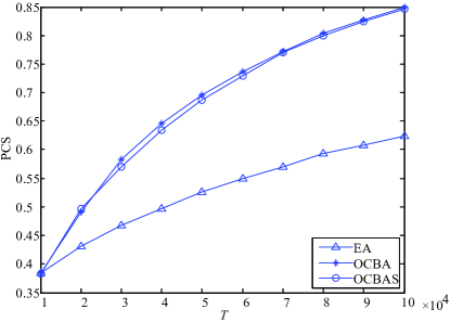
In this section, we present three groups of numerical experiments to demonstrate the performance of OCBAS. The first group discusses the impact of variance of individual simulation time (subsection IV-A). The second group discusses the impact of the correlation between individual simulation time and performance estimation (subsection IV-B). The third group is a smoke detection problem (subsection IV-C). Three methods are considered. First, equal allocation (EA), which equally allocates the simulation time among the designs. Second, OCBA, which iteratively allocates the number of replications among the designs[6]. Third, OCBAS, which iteratively allocates the simulation time among the designs.

IV-A Impact of Variance of Individual Simulation Time

Consider 10 designs with true performances $J_{i}=i-1$, $i=1,\ldots,10$. The performance estimation of all the designs have i.i.d. noise $N(0,6^{2})$. The individual simulation time of each designs are independent and all have the same variance. We consider two types of distributions of the simulation time. First, uniform distribution. We conduct 10 groups of experiments to consider 10 values of variances, in which the individual simulation time takes integer values from $[11-j,9+j]$ with equal probability, $j=1,\ldots,10$. Second, truncated discrete Gaussian distribution. We conduct another 10 groups of experiments, in which the individual simulation time of design $i$ satisfies $\Pr\{t_{i}=x\}\propto\Phi\left((x-i+1.5)/{j}\right)-\Phi\left((x-i+0.5)/{j}\right),x=1,\ldots,19;\Pr\{t_{i}=x\}=0,\text{ otherwise.}$ Note that different designs have different truncated discrete Gaussian distributions. Assume that the individual simulation time and performance estimation are independent. We apply EA, OCBA ($n_{0}=5,\Delta_{n}=10$, which means that each design is observed by 5 replications in the beginning and 10 replications are allocated among the designs in each iteration afterwards), and OCBAS ($T_{0}=50,\Delta_{T}=100$, which means that each design is observed using 50 units of time in the beginning and 100 units of simulation time are allocated among the designs in each iteration afterwards) under $T=1000,\ldots,10000$. Note that in each iteration of OCBA we calculate the additional number of simulations that are allocated to each design, which may take a random simulation time to complete. This is different from OCBAS, in which we allocate the simulation time directly. The PCS’s are estimated using 10000 replications and shown in Fig. 1. We make the following remarks.

Figure 1: PCS’s of EA, OCBA, and OCBAS of subsection IV-A (averaged over 10000 replications).

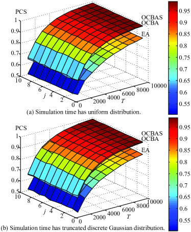
Remark 1. When the computing budget increases all three methods achieve higher PCS’s. This shows that all three methods can incrementally improve the PCS’s when more computing budget is available. This salient feature allows sequential allocations of the computing budget, which are usually preferred over fixed allocations beforehand in practice.

Remark 2. OCBAS substantially improves the PCS for a given $T$ (or in other words substantially saves the computing budget to achieve a given PCS).

Remark 3. OCBA and OCBAS achieve very close performances. The difference between their PCS’s are due to randomness of the experiments. This is because the allocation procedures of OCBA and OCBAS share the same spirit. The difference is that each iteration in OCBA fixes the total number of replications and thus takes stochastic time. But each iteration in OCBAS fixes the total simulation time. Then the total number of replications of a design becomes stochastic.

Remark 4. When the variance of individual simulation time increases, the PCS’s of OCBA and OCBAS do not change much. This is because each design is observed by more and more times when $T$ increases. So the variance of the simulation time does not significantly contribute to the performance estimation when the total simulation time is large, as shown in Lemma 3. Note that when the total simulation time is small, the variance of the simulation time matters. For example, when $T\leq 10$ (the mean value of each individual simulation), a larger variance allows to complete a simulation within $T$ with a larger probability. When the $T>10$, this impact of the variance reduces fast.

IV-B Correlated Simulation Time and Performance Estimation

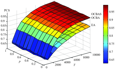
Consider 10 designs with true performances $J_{i}=i-1,i=1,\ldots,10$. The performance estimation of all the designs have i.i.d. noise $N(0,6^{2})$. The individual simulation time $t_{i}$ of design $i$ takes values of 5 and 15 with equal probability and is correlated with its performance observation noise $w_{i}$ as follows. If $w_{i}\geq 0$, then $t_{i}=15$ with probability (w.p.) $p$ and $t_{i}=5$ w.p. $1-p$, where $0\leq p\leq 1$ is a given constant. If $w_{i}<0$, then $t_{i}=15$ w.p. $1-p$ and $t_{i}=5$ w.p. $p$. The value of $p$ indicates the correlation between $t_{i}$ and $w_{i}$. In particular, $p=0$ means that $t_{i}$ and $w_{i}$ are purely negatively correlated; $p=1$ means that $t_{i}$ and $w_{i}$ are purely positively correlated; and $p=0.5$ means that $t_{i}$ and $w_{i}$ are independent. For $p=0,0.1,\ldots,1.0$ and $T=1000,\ldots,10000$, we apply EA, OCBA ($n_{0}=5,\Delta_{n}=10$), and OCBAS ($T_{0}=50,\Delta_{T}=100$) and estimate the PCS’s by 10000 replications (shown in Fig. 2). Remarks 1-3 also hold in this case. We can also see that the correlation $p$ does not affect PCS much.

Figure 2: PCS’s of EA, OCBA, and OCBAS of subsection IV-B (averaged over 10000 replications).

IV-C A Smoke Detection Problem

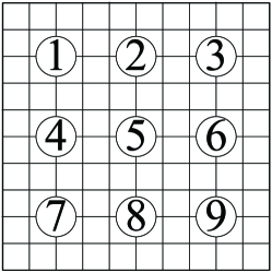
We compare three methods on a smoke detection problem in wireless sensor network. Consider an area of interest (AoI) with unit size as shown in Fig. 3, which is discretized into $11\times 11$ grids. A fire may be set at any point on the grid inside the AoI with equal probability. Once a fire is set on, it generates a smoke particle within each time slot. A smoke particle may walk to a neighboring grid in each time slot. There are at most four such neighboring grids corresponding to four directions. The probability to walk to one of the four grids is proportional to its distance to the fire source, i.e.,

$$\Pr\left\{x_{t+1}=x_{t}+1,y_{t+1}=y_{t}\right\} \propto d((x_{t}+1,y_{t}),(x_{0},y_{0})),$$

$$\Pr\left\{x_{t+1}=x_{t}-1,y_{t+1}=y_{t}\right\} \propto d((x_{t}-1,y_{t}),(x_{0},y_{0})),$$

$$\Pr\left\{x_{t+1}=x_{t},y_{t+1}=y_{t}+1\right\} \propto d((x_{t},y_{t}+1),(x_{0},y_{0})),$$

$$\Pr\left\{x_{t+1}=x_{t},y_{t+1}=y_{t}-1\right\} \propto d((x_{t},y_{t}-1),(x_{0},y_{0})),$$

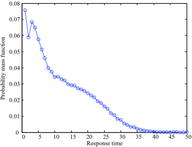
where $(x_{0},y_{0})$ represents the position of the fire source and $d(\cdot,\cdot)$ represents the distance between two positions. Once a particle walks to the boundary of AoI, it is bounced back. There are 3 sensors that can be allocated to the 9 positions marked by circles in Fig. 3. Once a smoke particle arrives at any of the three sensors, it is detected. The question is how to allocate the sensors to minimize the average detection time. It is easy to show that there are 84 allocations in total. Considering the symmetries, only 16 allocations need to be considered. The response time of the 16 designs are evaluated by 100000 independent replications and shown in Table I, where the designs are represented by the positions of the three sensors. Note that in each simulation the response time takes integer values. But the mean values of the response time take positive real numbers. As an example, we show the probability mass function of the response time of the first design (design 1,2,3) in Fig. 4, which is estimated by 100000 independent replications. Note that in this example we have $\hat{J}_{i}=t_{i}$, i.e., the performance estimation and individual simulation time are the same. This violates the assumption used in Theorem 2.

Figure 3: A smoke detection problem in wireless sensor network.

Figure 4: The probability mass function of the response time of the first design, estimated by 100000 replications.

TABLE I: True performances of the designs

Index	Design	Response time	Index	Design	Response time
1	1,2,3	11.5989	9	1,3,7	8.6777
2	1,2,4	10.6383	10	1,3,8	7.6482
3	1,2,5	9.3776	11	1,5,6	8.0903
4	1,2,6	9.3353	12	1,5,9	8.1355
5	1,2,7	9.7781	13	1,6,8	7.4699
6	1,2,8	8.2390	14	2,4,5	8.5127
7	1,2,9	8.7794	15	2,4,6	7.6968
8	1,3,5	8.6344	16	2,5,8	7.7671

The probability of correct selection of the three methods for $T=1\times 10^{4},2\times 10^{4},\ldots,1\times 10^{5}$ are evaluated using 10000 independent replications and shown in Fig. 5. Since each individual simulation of a design takes about 10 units of time (as shown in Table I) to make a fair comparison between OCBA and OCBAS, we use the following parameter settings. In OCBA, let $n_{0}=20$ and $\Delta_{n}=10$. In OCBAS, let $T_{0}=200$ and $\Delta_{T}=100$. Remarks 1-3 also hold in this case. We can see that OCBAS works well even when the performance estimation and individual simulation time are correlated.

Figure 5: PCS’s of EA, OCBA, and OCBAS of subsection IV-C (averaged over 10000 replications).

V Conclusion

In this paper, we consider the computing budget allocation for SBOs with stochastic simulation time and develop OCBAS to provide the allocation asymptotically optimally. The performance of OCBAS is demonstrated through two groups of academic examples and a smoke detection problem in wireless sensor network. The numerical results also show that OCBA for deterministic simulation time is robust even when the simulation time is stochastic. Note that the asymptotically optimal allocation of computing budget only depends on the mean value of the stochastic simulation time. Note that though we assume the performance estimate $\hat{J}_{i}$ and the simulation time for an individual replication $t_{i}$ are independent in section III, the numerical results in section IV show that OCBAS performs well when $\hat{J}_{i}$ and $t_{i}$ are correlated. Note that Lemma 3 shows that the performance estimator under stochastic simulation time can be well approximated by the performance estimator under deterministic simulation time. Replacing $n_{i}$ by $T_{i}/\mu_{i}$, OCBAS can be obtained straightforwardly from OCBA. Using Lemma 3, it is possible to extend OCBAS to handle multiple objective functions, simulation-based constraints, opportunity cost, and complexity preferences, following its according extensions in OCBA. That will be important future work. Note that when $N$ parallel computers are available, the total computing budget we can use will be improved from $T$ to $NT$. Both OCBA and OCBAS can be extended to this situation. But if each computer can simulate only a specific design, i.e., $N=k$, we usually have a constraint on the decision making time that is $\max_{i}{T_{i}}$. How to allocate computing budget according to this constraint is an interesting future research topic. We hope this work brings insights on addressing SBOs with stochastic simulation time in general.

References

- [1] R. E. Bechhofer, T. J. Santner, and D. Goldsman, Design and Analysis of Experiments for Statistical Selection, Screening and Multiple Comparisons, New York, NY: John Wiley & Sons, 1995.
- [2] J. R. Swisher, S. H. Jacobson, and E. Ycesan, “Discrete-event simulation optimization using ranking, selection, and multiple comparison procedures: A survey,” ACM Transactions on Modeling and Computer Simulation, vol. 13, pp. 134–154, 2003.
- [3] S.-H. Kim and B. L. Nelson, “Selecting the best system: Theory and methods,” in Proceedings of the 2003 Winter Simulation Conference, S. Chick, P. J. Sánchez, D. Ferrin, and D. J. Morrice, Eds., Piscataway, New Jersey, 2003, pp. 101–112.
- [4] C. H. Chen, “A lower bound for the correct subset-selection probability and its application to discrete event system simulations,” IEEE Trans. Autom. Control, vol. 41, pp. 1227–1231, 1996.
- [5] H.-C. Chen, C.-H. Chen, and E. Ycesan, “Computing efforts allocation for ordinal optimization and discrete event simulation,” IEEE Trans. Autom. Control, vol. 45, no. 5, pp. 960–964, May 2000.
- [6] C.-H. Chen, J. Lin, E. Ycesan, and S. E. Chick, “Simulation budget allocation for further enhancing the efficiency of ordinal optimization,” Discrete Event Dynamic Systems: Theory and Applications, vol. 10, pp. 251–270, 2000.
- [7] C. H. Chen and E. Ycesan, “An alternative simulation budget allocation scheme for efficient simulation,” International Journal of Simulation and Process Modeling, vol. 1, pp. 49–57, 2005.
- [8] C.-H. Chen, D. He, and M. Fu, “Efficient dynamic simulation allocation in ordinal optimization,” IEEE Trans. Autom. Control, vol. 51, no. 12, pp. 2005–2009, Dec. 2006.
- [9] S. Teng, L. H. Lee, and E. P. Chew, “Multi-objective ordinal optimization for simulation optimization problems,” Automatica, vol. 43, no. 11, pp. 1884–1895, Nov. 2007.
- [10] L. H. Lee, E. P. Chew, S. Teng, and D. Goldsman, “Finding the non-dominated pareto set for multi-objective simulation models,” IIE Transactions, vol. 42, pp. 656–674, 2010.
- [11] L. H. Lee, N. A. Pujowidianto, L. W. Li, C. H. Chen, and C. M. Yap, “Approximate simulation budget allocation for selecting the best design in the presence of stochasic constraints,” IEEE Trans. Autom. Control, to appear.
- [12] D. He, S. E. Chick, and C.-H. Chen, “Opportunity cost and ocba selection procedures in ordinal optimization for a fixed number of alternative systems,” IEEE Trans. Syst., Man, Cybern. C, vol. 37, no. 5, pp. 951–961, 2007.
- [13] S. Yan, E. Zhou, and C. H. Chen, “Efficient selection of a set of good enough designs with complexity preference,” IEEE Trans. Autom. Control, to appear.
- [14] C.-H. Chen and L.-H. Lee, Stochastic Simulation Optimization: An Optimal Computing Budget Allocation. Hackensack, NJ: World Scientific, 2011.
- [15] S. Andradóttir, “Simulation optimization,” in Handbook on Simulation, J. Banks, Ed. New York, NY: John Wiley and Sons, 1998, pp. 307–333.
- [16] M. C. Fu, “Optimization for simulation: Theory vs. practice,” INFORMS Journal on Computing, vol. 14, pp. 192–215, 2002.
- [17] J. R. Swisher, P. D. Hyden, S. H. Jacobson, and L. W. Schruben, “A survey of recent advances in discrete input parameter discrete-event simulation optimization,” IIE Transactions, vol. 36, pp. 591–600, 2004.
- [18] E. Tekin and I. Sabuncuoglu, “Simulation optimization: A comprehensive review on theory and applications,” IIE Transactions, vol. 36, pp. 1067–1081, 2004.
- [19] C. H. Chen, D. He, M. Fu, and L. H. Lee, “Efficient simulation budget allocation for selecting an optimal subset,” INFORMS Journal on Computing, vol. 20, no. 4, pp. 579–595, 2008.
- [20] D. Cox, Renewal Theory. London: Methuen & Co., 1970.