Search for giant planets in M67 I. Overview ††thanks: Based on observations collected at ESO, La Silla, Chile, OHP and HET.
Abstract
Context. Precise stellar radial velocities are used to search for massive (Jupiter masses or higher) exoplanets around the stars of the open cluster M67.
Aims. We aim to obtain a census of massive exoplanets in a cluster of solar metallicity and age in order to study the dependence of planet formation on stellar mass and to compare in detail the chemical composition of stars with and without planets. This first work presents the sample and the observations, discusses the cluster characteristics and the radial velocity (RV) distribution of the stars, and individuates the most likely planetary host candidates.
Methods. We observed a total of 88 main-sequence stars, subgiants, and giants all highly probable members of M67, using four telescopes and instrument combinations. We investigate whether exoplanets are present by obtaining radial velocities with precisions as good as 10 . To date, we have performed 680 single observations (Dec. 2011) and a preliminary analysis of data, spanning a period of up to eight years. After reducing all the observations to the HARPS zero point, the RV measurements for each star are used to evaluate the RV variability along the cluster color magnitude diagram.
Results. Although the sample was pre-selected to avoid the inclusion of binaries, we identify 11 previously unknown binary candidates. The RV variance (including the observational error) for the bulk of stars is almost constant with stellar magnitude (therefore stellar gravity) at 20 . Eleven stars clearly displayed larger RV variability and these are candidates to host long-term substellar companions. The average RV is also independent of the stellar magnitude and evolutionary status, confirming that the difference in gravitational redshift between giants and dwarfs is almost cancelled by the atmospheric motions. We use the subsample of solar-type stars to derive a precise true RV for this cluster (M67RV = 33.74 0.12 ) . The velocity dispersion is 0.54 for giants and 0.68 for dwarfs, substantially lower than reported in previous works. We finally create a catalog of binaries and use it to clean the color magnitude diagram (CMD). Isochrone fitting confirms an age of around 4 Gyr. Further cleaning of the CMD based on precise RV could establish M67 as a real benchmark for stellar evolutionary models.
Conclusions. By pushing the search for planets to the faintest possible magnitudes, it is possible to observe solar analogues in open clusters, and we propose 11 candidates to host substellar companions.
Key Words.:
Exoplanets – Open clusters and associations: individual: M67 – Stars: late-type – Stars: atmospheres – Techniques: radial velocities1 Introduction
1.1 Searching planets in open clusters
After the discovery of the first exoplanet around 51 Peg about 16 years ago (Mayor and Queloz 1995), more than 700 planets have been discovered, but a number of very basic questions still await answers, such as: how does the rate of planet formation depend on stellar metallicity and mass? Does planet formation strongly depend on the stellar environment?
Most exoplanets have been found around bright and nearby field stars that cover a very large range of stellar characteristics. These studies have many advantages, but the widely differing characteristics of field stars may also limit our capability to derive precise conclusions. For instance, it is puzzling that main-sequence stars hosting giant planets are metal rich (Gonzales et al. 1997, Santos et al. 2004), while evolved stars that host giant planets are not (Pasquini et al. 2007). Is this because of stellar pollution acting on main-sequence stars (e.g. Laughlin & Adams 1997), or because planet formation favors the birth of planets around more metallic stars (Pollack et al. 1996) ? Or maybe the metal-rich planet-hosting stars belong to an inner disk population, as proposed by Haywood (2009)? Are planet-hosting stars more depleted in Li than their non-hosting twins, as suggested by e.g. Israelian et al. (2009) (see however Baumann et al. 2010 for a different opinion) ? Or are the volatile elements depleted in the convective zones of stars that created rocky planets, as implied by the findings of Melendez et al. (2009) (see, however Gonzalez-Hernandez et al. 2010 for a different opinion)?
A large number of planets discovered around stars in open clusters would provide the perfect sample to answer all the above questions. Under the very reasonable assumption that open cluster stars have similar ages and chemical compositions (Pasquini et al. 2004, Randich et al. 2005, De Silva et al. 2007), a thorough, detailed chemical analysis of stars with and without planets belonging to the same cluster would provide direct answers to all the questions and hypotheses above, without any need for further speculation.
Similarly, it is now quite clear that stellar mass has a great influence on the frequency of giant planets (Lovis & Mayor 2007, Johnson et al. 2010), although the precise dependence of the planet rate on stellar mass is not yet known. In addition, a large number of giant planets around stars of open clusters, which have precisely determined masses, would provide an ideal database to study this dependence.
Finally, although most stars were born in stellar clusters and star associations, very little is known about the frequency of planetary systems in different environments, and on how their survival and evolution changes with it. A lot will be learned about this by directly imaging star forming regions, but the comparison between field and cluster statistics will help us to understand this point.
1.2 Previous searches
In spite of the importance of finding planets in open clusters, the literature on the subject is so far rather limited. The search for planets in open clusters with the RV technique has been limited to the studies of Paulson et al. (2002, 2004) around main-sequence stars of the Hyades, and the search for planets around evolved stars in a few clusters by Lovis & Mayor (2007) and around the Hyades giants (Sato et al. 2007). Paulson et al. did not find any evidence of short-period giant planets around the Hyades dwarfs, and excluded a high rate of hot jupiters in this high metallicity cluster. Several potential long-term candidates were present in their sample, but they did not perform any follow-up for longer periods.
Sato et al. (2007) found a long-period giant planet around one of the Hyades clump giants, and that there are only three such stars in this cluster led the authors to conclude that stellar mass has a significant influence on the giant planet rate. Finally, Lovis & Mayor (2007) collected RV observations of evolved stars in open clusters for several years. They found evidence of a couple of sub-stellar mass objects, and used statistical arguments to conclude that a higher stellar mass is more likely to promote the formation of massive planets.
Although the probability of finding a transiting exoplanet in an open cluster is rather low (van Saders & Gaudi 2011), open clusters (OC) have been targeted for extensive transit searches in the past few years(Bruntt et al. (2003), Street et al. (2003), von Braun et al. (2005), Bramich et al. (2005), Mochejska et al. (2005), Burke et al. (2006), Aigrain et al. (2006), et al. (2007, 2011), and Hartman et al. (2009, and references therein). However, only a handful of weak, unconfirmed candidates have been so far identified (Mochejska et al. 2006; et al. 2011).
Being much richer in stars than OCs, globular clusters (GCs) are of greater statistical significance, particularly in the case of a null detection (which always seems to be the case). Only a few GCs so far have been systematically searched for exoplanet transits. Among these, we may mention the ground-based campaigns targeting 47 Tucanae (Weldrake et al. 2005) and Centauri (Weldrake et al. 2008), both searching for hot-Jupiters around upper main-sequence stars in the outskirts of these two clusters, and both providing no significant exoplanet transit candidate.
The systematic photometric search that had placed the tightest constraints on the planet-frequency occurrence in a cluster, was that of Gilliland et al. (2000). This work was based on Hubble Space Telescope (HST) WFPC2 images of the dense core of 47 Tuc, which was monitored for 8.3 days during which about 34,000 upper main-sequence stars were observed. Gilliland et al. (2000) found no exoplanet transits, and concluded that the planet occurrence in 47 Tuc is smaller by a factor of ten than for field stars.
Nascimbeni et al. (2012) analyzed a similar HST data set (based this time on ACS/WFC images) in an outer field of the GC NGC 6397. For the first time, this work focused on searching for hot-Jupiters among low mass stars (K and M spectral types). Again, no high-significance planetary candidate was detected, but owing to the lower quality statistics no firm conclusion was reached about the occurrence of giant planets in M and K stars of NGC 6397.
The cause of the lack of close-in planets in GCs is not fully understood. Presumably the low metallicities and/or the dense environments interfere with planet formation, leading to orbital evolution to close-in positions, and/or planet survival.
1.3 Why a search in M67?
M67 is one of the most well-studied open clusters. It has been comprehensively observed to establish astrometric membership (Sanders 1977, Girard et al. 1989, Yadav et al. 2008), precise photometry (Montgomery et al. 1993, Sandquist 2004), and a rather precise RV and binary search (Mathieu et al. 1986, Melo et al. 2001, Pasquini et al. 2011). X-ray sources have been identified (Pasquini & Belloni 1998, Van den Berg et al. 2004), and was one of the first clusters for which observations of stellar oscillations were attempted (Gilliland et al. 1991). Its chemical composition and age are very close to solar values (Randich et al. 2006, Pace et al. 2008, Önehag et al. 2010) and it hosts very good candidates for solar twins (Pasquini et al. 2008, Önehag et al. 2010) .
For an open cluster, M67 is quite rich in stars, and its color magnitude diagram (CMD) is well populated in the main sequence, in the subgiant and red giant (RGB) branches. With a distance modulus of 9.63 (Pasquini et al. 2008) and a low reddening (E(B-V)=0.041, Taylor 2007), the solar stars have an apparent magnitude of V=14.58 and a (B-V) of 0.69 (Pasquini et al. 2008), and the cluster contains more than 100 stars brighter than this magnitude suitable for a RV planet search.
2 Sample and Observations
We selected stars that are proper motion members with a probability higher than 60 from Yadav et al. (2008) and also RV members, and unknown binaries from previous studies. In this context we recall the extended work of Mathieu and coworkers (Mathieu et al. 1986), who made a very complete RV survey of the evolved stars of M67 with a precision of a few hundred .
The majority of the other stars were selected following Pasquini et al. (2008), who used several VLT-FLAMES exposures for each star to classify suspected binaries. The full sample includes a total of 88 stars, from solar type (faintest is V15) to the tip of the RGB. The stars are rather faint for precise radial velocity observations, but a RV precision of 10 can be obtained for each measurement even for the faintest objects, with observations shorter than one hour at the ESO 3.6m telescope.
The bulk of the observations were carried out with HARPS at the ESO 3.6m telescope (Mayor et al. 2003), and this instrument is our reference for all the observations. Given the superior performances of HARPS, we concentrated mostly on the faintest objects with this facility.
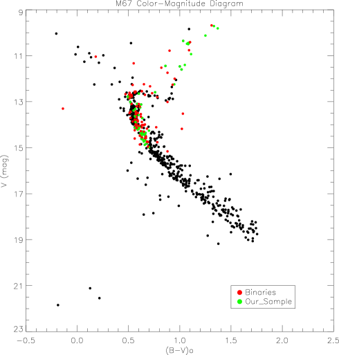
After the project started, we added the sample of evolved stars observed by CORALIE in the years 2003-2005, as part of a program of planet search of giants in open clusters (cfr. Lovis & Mayor 2007) . One limitation of our program is the sparse sampling frequency of the observations: typically a few nights/yr were awarded in the period January-April, and large gaps, longer than six months, are present between one season of observations and the next. We tried to gather HARPS observations for stars all over the CMD, to have enough points to derive proper zero-point offsets for the other instruments. Figure 1 presents the CMD of M67, using the photometry of Yadav et al. (2008) and stars with at least 60 membership from proper motions. The sample stars are marked in green, and spectroscopic binaries (see Table 6) in red.
2.1 HARPS observations
HARPS (Mayor et al. 2003) is the planet hunter at the ESO 3.6m telescope. In high accuracy mode (HAM) it has an aperture on the sky of one arcsecond, and a resolving power of 115000. The spectral range covered is 380-680 nm. In addition to be exceptionally stable, HARPS achieves the highest precision using the simultaneous calibration principle: the spectrum of a calibration (Th-Ar) source is recorded simultaneously with the stellar spectrum, with a second optical fibre. Since the M67 stars are quite faint for this instrument, we opted to use HARPS in the high efficiency mode: the fibre has a larger aperture on the sky (1.2 arcseconds, corresponding to R=90000) and is not equipped with an optical scrambler. This mode is limited to a precision of a few (5-7) , but it is 30-40 more efficient than the HAM mode. For our purposes this precision is sufficient, and the improved efficiency ensures that a high enough signal-to-noise (S/N) ratio can be obtained even for the faintest stars. As a rule of thumb we can consider that the precision of HARPS scales as (see below). Since the aim of this giant planet survey is a precision of the single measurement of 10 , it is possible to reach our goal with limited S/N observations, of on the order of S/N=10 at the peak of the signal. As a consequence, we can limit the integration time to less than one hour even for the faintest stars. Our HARPS spectra have typically a peak S/N of 15 for the faintest stars.
HARPS is equipped with a very powerful pipeline that provides on-line RV measurements, which are computed by cross correlating the stellar spectrum with a numerical template mask. This on-line pipeline also provides an associated RV error. For all of our stars, irrespective of the spectral type and luminosity, we used the solar template (G2V) mask.
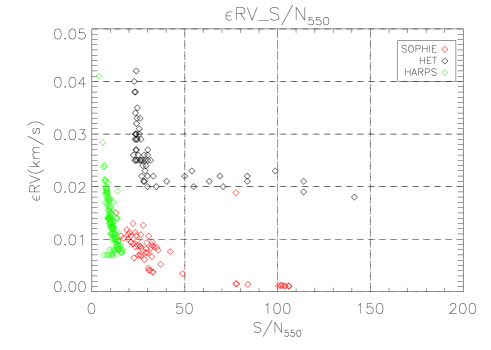
Figure 2 shows the error associated with the HARPS RV measurements versus (vs.) the S/N of the observations computed at the middle of echelle order 50 (555 nm) for the faintest stars of the sample (Vmag 14). The RV precision scales approximately as when expressed in and it levels off, as expected, at 8 for S/N above 13 for this order. In the figure, the uncertainty associated with each RV measurement is also given for SOPHIE (red) and HET (black). The magnitude range of the star sample is between 10.0-14.5 for SOPHIE and 9.8-14.0 for HET.
Between January 2008 and March 2011 we gathered 409 observations of 88 stars with HARPS, which represent the bulk of this work.
2.2 SOPHIE observations
SOPHIE is the planet hunter at the 1.93m OHP telescope (Bouchy et al. 2006). The instrument concept and data reduction is similar to that of HARPS; in high efficiency mode it has an aperture on the sky of three arcseconds with which a resolution of 40000 is obtained. In our first observing runs we observed all M67 stars with SOPHIE, including solar twins, but the smaller telescope diameter and the somewhat more critical weather conditions in winter at OHP than at La Silla, prompted our decision not to use this instrument further for the faintest objects.
We considered 34 M67 stars in common between our targets observed with SOPHIE and HARPS to compute the zero point between the two instruments. The comparison gives RV (SOPHIE)= RV HARPS -12.348.0 , with no dependence on the spectral type. This value is confirmed by the observations of the star 104Tau (HD32923), for which a difference of -11.407.0 between the two instruments is found (for a sample of 11 observations with HARPS and 5 with SOPHIE). We finally adopt a zero-point offset of -11.40 between SOPHIE and HARPS.
We analyze 78 SOPHIE observations of M67 stars with an associated precision of 12 . Since the observations with HARPS and the other instruments were not simultaneously acquired, we can assume that the precision with which the offsets are computed also includes the contribution from the intrinsic variability of the stars (and of course the photon and the instrumental noise).
2.3 CORALIE observations
CORALIE is located at the 1.2m Euler Swiss telescope at La Silla (Baranne et al. 1996). The M67 stars were observed between 2003 and 2005 in the framework of a larger program of search for planets around giants in open clusters (Lovis & Mayor 2007). The technique used to measure the RV in CORALIE observations is again the same as described for HARPS. As for the other instruments, the zero-point shift to HARPS was computed by using observations of stars in common to both instruments. Since the stars in common are only giants, it is expected that the intrinsic RV variability of these stars is larger than for main-sequence objects (Setiawan et al. 2004), and not negligible. We used ten stars in common between HARPS and CORALIE to evaluate the offset, obtaining RV(Coralie)= RV HARPS + 26.8 5.0 . We have so far gathered 123 observations for 17 giants with CORALIE with a precision associated with these observations of 20 .
2.4 HET Observations
HRS, mounted on the 10 m HET telescope (Tull 1998), was the last instrument used in our survey. We were granted 70 observing runs in service mode between November 2010-April 2011. Each run consisted of two exposures of 1320 s and counts as one observation. The configuration was set to a wavelength range between 407.6 nm and 787.5 nm with a central wavelength at 593.6 nm and a resolving power of R=60000. We were able to observe 13 objects selected from our sample with 9.0Vmag14.6. The S/N for the faintest stars is 10. The radial velocities were computed using a series dedicated routines (Cappetta et al. 2012, in preparation). The different steps include the wavelength calibration using a Th-Ar lamp exposure performed before and after each stellar spectrum, the normalization of the spectra, the cleaning of cosmic rays and both, telluric and sky lines, the computation of the heliocentric corrections and finally the cross-correlation of the spectrum with a G2 star template. We used the multiple exposures of the same star to estimate the typical error bar associated with the HET observations, finding an error of 25 .
When considering the different analysis used for the HET data with respect to the other instruments, it is unsurprising to find a larger offset with respect to HARPS for HRS than for the other instruments: RV (HRS)= RV(HARPS)+ 242.0 12 ( eight stars were used for the comparison).
| Istrument | HARPS | SOPHIE | HET | CORALIE |
|---|---|---|---|---|
| N obs.Stars | 88 | 54 | 15 | 17 |
| Observations | 409 | 78 | 70 | 123 |
| MS stars | 58 | 42 | 7 | |
| TO stars | 7 | 2 | 4 | |
| G stars | 23 | 10 | 4 | 17 |
| Period | 2008-2011 | 2008-2011 | 2010-2011 | 2003-2005 |

3 Results
Once corrected to the zero points of HARPS, all the observations of each star were collected and analyzed together. Table 5 summarizes the main data for the observed stars. In addition to the basic stellar parameters, the number of observations per star is given, for each spectrograph and as a total.
We have obtained, on average, 7 observations/star, but this ranges from a minimum of 2 to more than 20 (see Table 5). The histogram showing the number of observations/star is given in Figure 3. We performed a series of Monte Carlo simulations to establish the minimum number of observations/star that we need to exclude the presence of hot Jupiters at high confidence. The preliminary results indicate that a final number of at least 9 observations/star should be reached (Brucalassi et al. 2012, in preparation).
In the last two columns of Table5 the mean stellar RV of each star is given, together with the RV dispersion. Individual RV measurements will be provided in a forthcoming paper devoted to the detailed discussion of the planets’ host candidates and to discussion of the presence of hot Jupiters (Brucalassi et al. 2012, in preparation).
3.1 Binaries and CMD
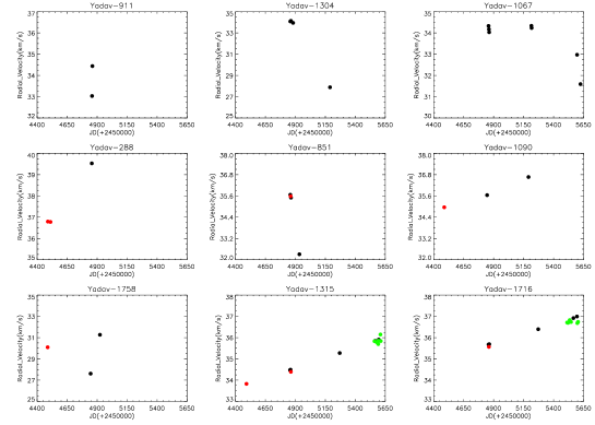
One of the first findings of our survey is that, despite all the stars having been previously observed and found to have no evidence of companions, 11 stars in the original sample of 88 (13) show RV variations that are too large to be produced by an exoplanet, or by a non-stellar object. We considered as binary candidates all the stars displaying a peak-to-peak RV amplitude of at least 1.7 . Considering half of the difference as a lower limit to the orbital semi-amplitude, this amplitude corresponds to a companion of 15 Jupiter masses on a 30 day period for a circular orbit around a star of 1.2 solar masses. The RV range spanned by these stars is so large that planetary companions can be excluded, as can be seen from Figure 4, where the RV measurements for 9 of the binary candidates are shown. The binary/long-term RV variable nature of 7 of them was confirmed by D. Latham (private communication), who is performing a long-term RV monitoring of more than 400 M67 stars (Latham 2006).
| Object | V | B-V | RV | RV |
|---|---|---|---|---|
| Y | ||||
| Y | ||||
| Y | ||||
| Y | ||||
| Y | ||||
| Y | ||||
| Y | ||||
| Y | ||||
| Y | ||||
| Y | ||||
| S |
The measurements are also given in table 2, which is available in electronic form. These stars are binary candidates, and were not observed after a large variation of their RV was measured. Given that these stars are high-probability M67 proper-motion members, and that their RV is close to that of the cluster, it is very likely that they are spectroscopic binaries belonging to the cluster.
Two stars (S815 and S1197, cf Table 5) show peak to peak RV variations of the order of 700 /ms ; they are retained in the single star sample, although the amplitude of the RV variation is possibly too high to host a planet.
In the process of evaluating the effects of binaries in M67 CMD, we found that binaries are identified in many works in the literature and sometimes different names are used; in addition several works have been published after the compilation of Sandquist (2004). We therefore opted to create a new catalog of binaries in M67 that includes our candidates, binaries from the literature, as well as binary candidates from X-ray observations. The catalog is given in Table 6, with reference to the original studies.
The binary stars from Table6 are plotted in Figure 1 as red points. The high percentage of binaries in M67 is unsurprising, given that to retain the stars for such a long time, M67 has the most massive stars in the core, and some mass segregation has occurred.
A complete census of the binaries in M67 is helpful because this cluster can be used to test the effects of several mechanisms debated in stellar evolution, such as diffusion and overshooting (see e.g. the discussion in Magic et al. 2010). Cleaning of the CMD is especially important in the region of the turnoff, because, as is clear in Figure 5, in that region binaries cannot be photometrically distinguished from single main-sequence stars. They separate more clearly along the main sequence, where a separate, detached binary sequence is present, although several fainter binaries lie on the main sequence and are photometrically indistinguishable from single stars in the CMD.
In his extensive study of M67, Sandquist (2004) created one table containing the fiducial sample of single stars and a second table with a list of interesting or peculiar stars. In the first list, 11 stars are indicated as possible binaries according to our catalog (S1305, 1458, 990, 1300, 1075, 1201, 982, 1102, 1452, 951, 820), and one star (S1197) has large RV variations. Among these 11 binary candidates, some have weak evidence coming from a few FEROS or FLAMES multiple spectra, which had a limited precision. For instance star S1305, a low-RGB star, is indicated as a suspected binary in Pasquini et al. 2011, but is not confirmed by our higher precision measurements (cfr. Table5). Other Sandquist’ single-star sequence fiducial stars (e.g. S982, 1201, 1452) are, on the other hand, confirmed to be binaries by our high-precision RV measurements.
Three stars of the Sandquist ’unusual stars’ table are confirmed to be RV multiple candidates according to Table 6 (S1292, S816, S1011).
The above results show that, in spite of the large efforts to clean the CMD of M67, a number of unknown binaries are still present and the detailed comparisons required to distinguish between different potential mechanisms (Magic et al. 2010) could strongly benefit from additional cleaning, in particular around the turnoff.
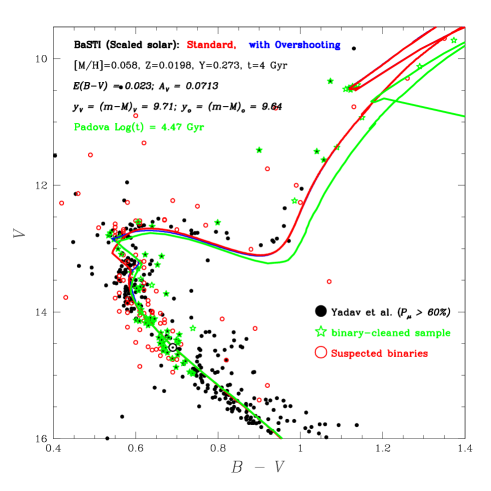
In Figure 5, we show the observed region of the CMD with the isochrones from Pietrinferni et al.( 2004), with and without overshooting. In this CMD, we also indicate the position of the solar analog, as determined in Pasquini et al. 2008, and we impose that the tracks appropriately fit this point, in addition to the rest of the CMD. The 4 Gyr track with moderate overshooting seems to most closely represent the data. In the same figure, we also superimpose the Padova isochrones, with solar metallicity, age 4.47Gyr, and Y=0.26 (Girardi et al. 2000, as from Girardi web page). The isochrone fits the turnoff very well, but produces a RGB and clump that are too red. The mismatch is not dramatic and may indicate some problem in either the bolometric correction used or some of the free parameters adopted (e.g. mixing length). We note that for both sets of isochrones a slightly lower reddening (E(B-V)=0.02 instead of 0.041 (Taylor 2007)) is needed to match the colors of the turnoff. We also note that there are a number of stars, apparently with constant RVs, and a high probability of proper motion membership, that are above the main sequence.
This analysis confirms that, in addition to its extraordinarily similar abundance pattern, M67 has an age compatible with that of the Sun.
Given these similarities and that the solar birthplace has not yet been identified, it is natural to ask whether M67 and the Sun were associated in the past. This problem was exhaustively studied by Pichardo et al.(2012), who performed a full set of dynamical simulations, excluding that M67 and the Sun were born in the same cloud. This result leaves us therefore with a question mark about the birthplace of the Sun and might challenge the validity of chemical tagging, which associates stars with either clusters or associations based on the similarity of their chemical compositions (see e.g. Freeman and Bland-Hawthorn 2002).
3.2 Radial velocity variability
We first investigate the observed RV variability along the CMD. Since all the stars belong to the cluster with high probability, we have the unique opportunity to study how RV variability changes along the CMD diagram, for a given chemical composition and age. In addition, a diagram with RV variability vs. magnitude would immediately highlight any possible ’outliers’, which would be the most obvious hosts of exoplanets.
Setiawan et al. (2004) and Hekker and Melendez (2007) shwed that the intrinsic RV variability of giants increases with stellar luminosity and becomes large for bright, low-gravity giants. Since we cover a six magnitude interval, it could be useful to determine for each magnitude or evolutionary status a typical average RV variability. This quantity should depend solely on both, the intrinsic stellar RV variability and the RV measurement error (typical photon errors associated with the bright stars are smaller because faint star observations are limited by photon noise).

Figure 6 shows the rms RV vs. V diagram for 75 single stars. Binary candidates have been excluded, and the two stars (S815 and S1197) with high RV variability are not shown.
Some of the stars with very little or no RV variability have very few observational points, and their small scatter is very likely the result of our low data statistics. The increase in RV scatter with stellar luminosity observed in field stars (Setiawan et al. 2004) is not evident in our sample. There is a possible hint of an increase in the range of magnitudes 12V14, but the RV variability does not increase further for the more luminous stars.
As a general conclusion, we can say that the RV variability shown in Figure 6 is basically constant at 20 (), independent of the stellar magnitude. The bulk of our observations have a RV variability that is well represented by a Gaussian distribution centered at 20 of width = 10 .
The unexpected flatness of the RV variability with magnitude is most likely due to the combination of two effects. In evolved stars, some measurable stellar RV variability is present, while for the faint main-sequence stars the uncertainty in the measurements increases because of the limited S/N.
To investigate these points, in Figure 7 we plot the RV variability as a function of the stellar luminosity to mass ratio (L/M). According to Kjelsden and Bedding (1995) the RV jitter induced by solar oscillations is expected to grow according to the law RV 0.23*L/M (with RV expressed in ). This law is represented by the continuous line. Figure 7 illustrates the very good agreement between this scaling law and the RV variability of evolved stars in M67. The continuous line remains just below the measurements, but this does not take into account that the measurements, in addition to the stellar intrinsic variability, include measurement uncertainties that are not negligible. A fit to the evolved star data (L/M 5) gives = 0.25 L/M + 9.3 ( ), which is shown by the dashed line in Figure 7. The observations and the predictions therefore match quite well, when the measurement errors are considered. We note that this comparison implies that the oscillation RV amplitude and its variations are of comparable size. More precise RV measurements would allow us to quantitatively investigate this point in more detail. We conclude that the M67 evolved stars show signs of intrinsic RV variability and that for most of the evolved stars the observed RV variability is consistent with that expected from the Kjelsen and Bedding (1995) scaling law for solar-type oscillations.
As far as the lower main sequence is concerned, the behavior of the faint stars in our sample (which are also the least massive ones) is quite interesting, because if the RV variability observed were induced by substellar companions, this would already indicate a correlation between planet frequency and mass in M67. There are good arguments to believe that an RV variability as large as 20 cannot be caused by intrinsic stellar noise, because stellar noise for solar stars scales with activity and therefore age, and M67 is almost as old as the Sun (see e.g. Saar et al. 1998, Dumusque et al. 2011). On the other hand we have seen that the uncertainties in the RV measurements of faint stars is above 10 (cfr Figure 2) but well below 20 . We investigated whether other instrumental effects, not included in the data analysis, could affect the RV measurement precision at low count levels. At least two effects could influence the observations, and we investigated whether our measurements depend on observational parameters, such as the observed flux or airmass. A dependence on flux could be induced, for instance, by CCD transfer inefficiency, which has been reported to be high in SOPHIE (Bouchy et al. 2009). A dependence of RV on airmass could instead indicate that some systematic effects are induced by the HARPS atmospheric dispersion compensator at high airmass or by the guiding system of the telescope. For every solar star, we therefore computed the RV of each observation with respect to the average stellar radial velocity, and analyzed all the measurements of all stars together, as functions of counts and airmass. No trend is present, as is clear from Figure 8, where the RV is plotted vs. the square of the S/N at 550 nm. We conclude therefore that these two quantities do not affect our measurements in an appreciable way. We note that in these comparisons only the HARPS data have been used, because they by far dominate the faint star statistics.


With a RV variability for the whole sample centered at 20 and a width of 10 , we can safely assume that stars with a RV variability at or above 50 are very good candidates for low mass companion hosts. A number of stars (9) stand out clearly from the general constant trend of Figure 3, showing a RV variability of 50 or larger. These stars (plus S815, and S1197, which are not included in the figure) are candidates to host giant planets or substellar objects. Another 6 candidates have smaller, but still interestingly large RV variability, and deserve to be investigated further. The list of the most likely 11 candidates is given in Table 3.
| Object | V | B-V | RV | RV |
|---|---|---|---|---|
| Y | ||||
| Y | ||||
| Y | ||||
| Y | ||||
| Y | ||||
| Y | ||||
| Y | ||||
| Y | ||||
| S | ||||
| S |
Several stars show clear long trends of RV variability compatible with the presence of a planet, but the baseline is not yet long enough to determine the nature of the companion. More RV points are required and are being acquired. A full analysis of the data of our completed survey will be published elsewhere (Brucalassi et al. 2012).
The large scatter in the radial velocities, in excess of the measurement errors, may indicate that more stars, in addition to those indicated in Table 3 are suitable candidates for hosting planets.
Keeping in mind that we are only sensitive to rather massive planets, we find it interesting that our candidates should all have long orbital periods. Mayor et al. (2011) found clear evidence that the most massive planets tend to have long orbits, which is perfectly in line with our results. Similarly, if all 9 candidates were planets, they would correspond to a frequency of giant planets of 13, which agrees with the rate of giant planets found by Mayor et al. (2011) and by Döllinger et al. (2012, in preparation) around evolved stars.
3.3 Gravitational redshift in M67 and cluster radial velocity
Pasquini et al. (2011) used FEROS and literature observations of M67 stars to investigate whether gravitational redshift could be detected in the stars of this cluster, by comparing the measured RV of the cluster dwarfs and giants. Their adopted technique assumes that the subsamples of cluster stars share the same cluster RV, irrespective of their mass and evolutionary status.
These authors found that, when using the radial velocities derived from cross correlation masks, there was no evidence of gravitational reddening: giants and dwarfs have, within the RV uncertainties, the same radial velocity. They also showed that this behavior is compatible with the shifts and asymmetries of spectral lines predicted by 3D models. They found in addition that M67 giants are dynamically cooler than dwarfs.
Although our sample is smaller than the one used by Pasquini et al. (2011), our RV data are 10-20 times more precise, and, in addition, the many observations acquired have allowed us to eliminate several binaries, which would cause the cluster to appear dynamically hotter and perhaps introduce a skewness in the RV distribution. Since all our newly discovered binaries are on the main sequence, they might have influenced the conclusions about the dynamical status of the cluster, making the dwarfs appear dynamically hotter. Pasquini et al. (2011) derived a = 680 and a = 900 and estimated that their FEROS RV precision is of 300 . The RV precision of our measurements is more than one order of magnitude more accurate than these values. For the first time we have gathered a sample of stars in M67 whose RV measurement errors are definitely negligible with respect to the cluster dynamics.
Figure 9 shows the distribution of stellar RV vs. stellar magnitude, and Figure 10 the same RV but vs. the ratio of stellar mass to radius (see Pasquini et al. 2011 for details). If gravitational reddening were the only process acting, we would expect a dependence of RV = RV0 + 0.632(M/R).

There is clearly no significant dependence of RV on either magnitude or M/R, confirming the FEROS results of Pasquini et al. 2011. A least squares fit to the V-RV diagram gives , where the angular coefficient is closely compatible with zero (error is 0.047).
The average radial velocity of all stars is 33.724 kms-1, with a dispersion of 0.646 . By dividing the sample into “giants” and “dwarfs” at B-V=0.7, we find = 540 ( 90 , 18 stars, v=33.67) and = 680 ( , 59 stars, v=33.74).
By computing the ratio mass to radius for each star (cf. Pasquini et al. 2011) we find that RV depends only very slightly on M/R, with an angular coefficient of 0.096 that is much smaller than the 0.6 expected from gravitational reddening (cf. Figure 6), confirming the results of Pasquini et al. (2011).
In the future we plan to merge all the HARPS spectra acquired for each star to perform a detailed spectroscopic study, including chemical abundance and line-shift analyses.

Since the present RV measurements are much more precise than in the past, the RV dispersion is smaller than that found by Pasquini et al. (2011). If we attribute the difference between the giant dispersion found in Pasquini et al. (2011) (680 ) and that found in this paper (540 ) entirely to the FEROS RV uncertainty, , this would be approximately 400 . The value is slightly larger than the FEROS errors estimated by Pasquini et al. (2011) (300 ), but it is not unreasonable when considering that for most FEROS stars only one observation was available, so some intrinsic stellar RV variability should also contribute to the difference.
Finally we use the solar-stars radial velocities to compute the true radial velocity of the cluster. We consider that, what is commonly called ’radial velocity’ is the measure of the center of the cross-correlation function (CCF) between the stellar lines and a digital mask that in our case is based on the solar spectrum. This implies that the measured Doppler velocity includes the stellar radial velocity, the effects of stellar atmospheres, and the errors in the positioning of the lines in the digital mask (see Lidegren and Dravins 2003).
Our observations span the whole cluster and include many solar-type stars. This allows us to properly convert the measured Doppler shifts of the single stars into a measurement of the true radial velocity of the cluster. We therefore analyze only the 36 stars most similar to the Sun, in the range 14.0 V 15. The magnitude of the closest solar analogs is V14.58 (Pasquini et al. 2008, Öhenaag 2010). The only two underlying hypotheses are that as a group these stars share the same cluster velocity and that they are representative of the solar spectrum. The average Doppler shifts for the CCF of these 36 stars is M67Ds=33.83 kms-1, with a = 712 , which implies that the associated uncertainty for M67Ds is 118 .
To compute the true radial velocity of the cluster, we must correct in addition for the zero-point offset of the G2 mask used. We did this by using the asteroid observations of Ceres obtained by HARPS and described in Molaro et al. (2008) and Molaro & Centurion (2011). The expected radial velocity of the asteroids with respect to La Silla can be computed rather accurately, and the difference between the computed and the measured radial velocity gives the zero offset of the mask from the solar spectrum. With this procedure, we can pass from Doppler shift measurements to the true radial velocity of solar stars.
Table 4 shows the results of the expected vs. measured Ceres radial velocity: the two results are very consistent, to the order of 1 , indicating a shift for the mask of 94.5 . This velocity must be subtracted from the measured M67Ds to obtain the true cluster radial velocity, which is therefore M67RV = 33.74 kms-1.
| JD | Expected RV | Measured RV | V |
|---|---|---|---|
| Mid-exposure | kms-1 | kms-1 | |
| 2453932.837256 | -10.832 | -10.738 | 94 |
| 2453877.919808 | -22.017 | -21.922 | 95 |
We note that the error given by the zero-point correction of the mask is completely negligible compared to the uncertainty introduced by the cluster internal motions. Therefore, by enlarging the sample of solar-type stars, the final error could easily be diminished and very precise measurements of the radial velocity of the cluster could be obtained. This mask offset can also be applied to solar-type field stars to derive their true radial velocities, and this method could be extended to determine precise RV offsets as a function of stellar gravity and temperature for solar metallicity stars. Finally, true radial velocities could then be determined for field stars of different spectral types.
Our new data confirm that the dwarfs are dynamically hotter (ratio 1.25) than the giants in this cluster. All the derived parameters agree very well with those computed by the maximum likelihood estimation in Pasquini et al. (2011).
4 Conclusions
We have presented a long-term search program for giant planets in the solar-age, solar-metallicity open cluster M67.
We have used four different instruments, and, after finding proper zero-point corrections to HARPS, we have analyzed 680 observations for 88 stars. Twelve new binaries have been identified and we have created a catalog of known binaries in M67, which we have used to clean the cluster CMD. We have found that the CMD is well represented by tracks of solar age with some overshooting. The observed RV variability does not depend very strongly on the stellar magnitude. The evolved stars show a RV variability that follows the Kjeldsen and Bedding (1995) scaling law for solar oscillations quite closely, while the RV variability for the main-sequence stars is dominated by the RV measurement uncertainties.
Eleven stars show long-term RV variability in a range that make them interesting candidates for exoplanet hosts. If confirmed, their long period and fraction would agree with recently derived statistics for field stars (Mayor et al. 2011).
We finally used our precise RV measurements to confirm that no gravitational redshift is measured between M67 giants and dwarfs, confirming that the velocity dispersion of main-sequence stars is larger than that of giants (680 vs. 540 , respectively). We determined the zero-point shift of the G2 mask of HARPS and by using the solar stars we determined a true M67 radial velocity of 33.740.12 kms-1.
We have shown that the search for planets in open clusters is a really powerful tool for investigating a large number of questions related to planet formation and stellar evolution. The new generation of spectrographs, such as ESPRESSO (Pasquini et al. 2009), will make this search more effective and precise.
Acknowledgements.
LPA thanks ESO DGDF and the kind hospitality of UFRN(Br); he also thanks Paul Bristow for a careful reading of the manuscript. RPS acknowledges the support of RoPACS during this research, a Marie Curie Initial Training Network funded by the European Commissions Seventh Framework Programme. The Hobby Eberly Telescope (HET) is a joint project of the University of Texas at Austin, the Pennsylvania State University, Stanford University, Ludwig Maximilians Universität Muenchen, and Georg-August Universität Goettingen. We are grateful to Programme National de Physique Stellaire and Programme National de Planetologie of the Institut de Science de l’Univers of CNRS for allocating and supporting the SOPHIE observations.References
- Aigrain et al. (2006) Aigrain, S.; Irwin, J.; Hodgkin, S.et al. 2006, in “Tenth Anniversary of 51 Peg-b: Status of and prospects for hot Jupiter studies.”, L. Arnold, F. Bouchy and C. Moutou eds. p.181
- Baranne et al. (1996) Baranne, A., Queloz, D., Mayor, M., & et al. 1996, A&AS, 119, 373
- Baumann et al. (2010) Baumann, P., Ramirez, I. et al. 2010, A&A 519, 87
- Belloni et al. (1998) Belloni, T., Verbunt, F., Mathieu, R. D. 1998, A&A 339, 431
- Bouchy et al. (2006) Bouchy, F., and the SOPHIE team, 2006, in “ Tenth Anniversary of 51 Peg-b: Status of and prospects for hot Jupiter studies”, L. Arnold, F. Bouchy, and C. Moutou eds. p. 319
- Bouchy et al. (2009) Bouchy, F.; Isambert, J.; Lovis, C.; Boisse, I.; Figueira, P. et al. 2009, EAS Publication Series 37, 247
- Bramich et al. (2005) Bramich, D. M.; Horne, Keith; Bond, I. A. et al. 2005, MNRAS 359, 1096
- Bruntt et al. (2003) Bruntt, H.; Grundahl, F.; Tingley, B.; Frandsen, S.; Stetson, P. B.; Thomsen, B. 2003, A&A 410, 323
- Burke et al. (2006) Burke, C.J.; Gaudi, B. Scott; DePoy, D. L.; Pogge, R.W. 2006, ApJ 132, 210
- De Silva et al. (2007) De Silva, G., Freeman, K.C. et al. 2007, AJ 133, 1161
- Dumusque et al. (2011) Dumusque, X., Lovis, C. et al. 2011, A&A 525, 140
- Freeman& Bland-Hawthorn (2002) Freeman, K., & Bland-Hawthorn, J. 2002, ARA&A, 40, 487
- Gilliland et al. (1991) Gilliland, R.L., Brown, T.M. et al. AJ 101, 541
- Gilliland et al. (2000) Gilliland, R.L.; Brown, T. M.; Guhathakurta, P. et al. 2000, 545, L47
- Girard et al. (1989) Girard, T. M., Grundy, W. M., Lopez, C. E., & van Altena, W. F. 1989, AJ, 98, 227
- Girardi et al. (2000) Girardi, L., Bressan, A., Bertelli, G., & Chiosi, C. 2000, A&AS, 141, 371
- Gonzalez (1997) Gonzalez, G. et al. 1997, MNRAS, 285, 403
- Gonzalez Hernandez et al. (2010) Gonzalez Hernandez, J.I., Israelian, G. et al. 2010, A&A 720, 1592
- Hartman et al. (2009) Hartman, J. D.; Gaudi, B. S.; Holman, M. J. 2009, ApJ 695, 336
- Haywood (2009) Haywood, M. 2009, ApJ 698, L1
- Hekker & Melendez (2007) Hekker, S.; Meléndez, J. 2007, A&A 475, 1003
- Israelian et al. (2009) Israelian, G. Delgado Mena,E. et al. Nature 462, 189
- Johnson et al. (2010) Johnson, J.A., Aller, K.M. et al. 2010, PASP 122, 905
- Kjelsden & Bedding (1995) Kjeldsen, H., Bedding, T.R. A&A 293, 87
- Latham et al. (1992) Latham, D. W., Mathieu, R. D., Milone, A. A. E., & Davis, R. J. 1992, IAU Coll. 135: Complementary Approaches to Double and Multiple Star Research, ed. H. A. McAlister & W. I. Hartkopf, ASPC, 32, 155
- Latham (2006) Latham, D.W. 2006, in ”Modelling Dense Stellar Systems, 26th meeting of the IAU, Joint Discussion 14, 22-23 August 2006”, IAUJD 14, 8L
- Laughlin & Adams (1996) Laughlin, G., & Adams, F. C. 1997, ApJ, 491, L51
- Lindegren & Dravins (2003) Lindegren, L., & Dravins, D. 2003, A&A, 401, 1185
- Lovis & Mayor (2007) Lovis, C. Mayor, M. 2007, A&A 472, 657
- Magic et al. (2011) Magic, Z., Serenelli, A. et al. 2010, ApJ 718,1378
- Mathieu et al. (1986) Mathieu, R. D., Latham, D. W., Griffin, R. F., & Gunn, J. E. 1986, AJ, 92, 1100
- Mathieu et al. (1990) Mathieu, R. D., Latham, D. W., Griffin, R. F. 1990, AJ, 100, 1859
- Mayor & Queloz (1995) Mayor, M. Queloz, D. 1995, Nature 378, 355
- Mayor M. et al. (2003) Mayor, M., Pepe, F. et al. 2003, The Messenger 114, 20
- Mayor M. et al. (2011) Mayor, M., Marmier, M., Lovis, C. et al. 2011 2011arXiv1109.2497M
- Melendez et al. (2009) Melendez, J. et al. 2009, ApJ 704, L66
- Melo et al. (2001) Melo, C. H. F., Pasquini, L., & De Medeiros, J. R. 2001, A&A, 375, 851
- Mochejska et al. (2005) Mochejska, B. J.; Stanek, K. Z.; Sasselov, D. D. et al. 2006, AJ, 129, 2856
- Mochejska et al. (2006) Mochejska, B. J.; Stanek, K. Z.; Sasselov, D. D. et al. 2006, AJ, 131, 1090
- Molaro et al. (2008) Molaro, P., Levshakov, S. et al. 2008, A&A 481, 559
- Molaro & Centurion (2011) Molaro, P., Centurion, M. 2011, A&A 525, 74
- Montalto et al. (2007) Montalto , M.; Piotto, G.; Desidera, S. et al. 2006 A&A 470, 1137
- Montalto et al. (2011) Montalto, M.; Villanova, S.; Koppenhoefer, J., et al. 2011 A&A 535, 39
- Montgomery et al. (1993) Montgomery, K. A., Marschall, L. A., & Janes, K. A. 1993, AJ, 106, 181
- Nascimbeni et al. (2012) Nascimbeni, V.; Bedin, L. R.; Piotto, G.; De Marchi, F.; Rich, R. M. 2012, 2012arXiv1202.5112N
- Önehag et al (2011) Önehag, A.; Korn, A.; Gustafsson, B.; Stempels, E.; Vandenberg, D. A. A&A 528, 85
- Pace et al. (2008) Pace, G., Pasquini, L., & François, P. 2008, A&A, 489, 403
- Pasquini & Belloni (1998) Pasquini, L., Belloni T. 1998, A&A 336, 902
- Pasquini et al. (2004) Pasquini, L., Randich, S., Zoccali, M.,& et al. 2004, A&A, 424, 951
- Pasquini et al. (2007) Pasquini, L., Döllinger, M. et al. 2007, A&A 473, 979
- Pasquini et al. (2008) Pasquini, L., Biazzo, K., Bonifacio, P., Randich, S., & Bedin, L. R. 2008, A&A, 489, 677
- Pasquini et al. (2009) Pasquini, L., Manescau. A. et al. 2009, in ”Science with the VLT in the ELT Era” Astrophysics and Space Science Proceedings, Volume . ISBN 978-1-4020-9189-6. Springer, p. 395
- Pasquini et al. (2011) Pasquini, L., Melo, C. et al. 2011, A&A 526, 127
- Paulson et al. (2002) Paulson, D.K. et al. 2002, AJ 124, 572
- Paulson et al. (2004) Paulson, D.K. et al. 2004, AJ 127, 1644
- Pietrinferni, A. et al. (2004) Pietrinferni, et al. 2004. ApJ 612, 168
- Pichardo et al. (2012) Pichardo, B. Moreno, E. et al. 2012, ApJ, in the press
- Pollack et al. (1996) Pollack, J. B., Hubickyj, O., Bodenheimer, P., et al. 1996, Icarus, 124, 62
- Randich et al. (2005) Randich, S., Bragaglia, A. et al. 2005, The Messenger, 121, 18
- Randich et al. (2006) Randich, S., Sestito, P., Primas, F., Pallavicini, R., & Pasquini, L. 2006, A&A, 450, 557
- Saar et al. (1998) Saar, S.H., Butler, R.P., Marcy, J.W. 1998, ApJ 498, L153
- Sanders (1977) Sanders, W. L. 1977, A&AS, 27, 89
- Santos et al. (2004) Santos, N., Israelian, G., Mayor, M. 2004, A&A 415, 1153
- Sandquist & Shetrone (2003) Sandquist, E. L., Shetrone, M. D. 2003, AJ 125, 2173
- Sandquist et al. (2003) Sandquist, E.L., Latham, D. W., et al. 2003, AJ 125, 810
- Sandquist (2004) Sandquist, E. L. 2004, MNRAS, 347, 101
- Sato et al. (2007) Sato, B., Izumiura, H. et al. 2007 ApJ, 661, 527
- Setiawan et al. (2004) Setiawan, J., Pasquini, L., da Silva, L., & et al. 2004, A&A, 421, 241
- Street et al. (2003) Street, R. A.; Horne, K.; Lister, T. A. et al. 2003, MNRAS 340, 1287
- Taylor (2007) Taylor, B. J. 2007, AJ, 133, 370
- Tull (1998) Tull, R.G. 1998, Proceedings SPIE 3355, 387
- Yadav et al. (2008) Yadav, R.K.S., Bedin, L.R. et al. 2008, A&A 484, 609
- van den Berg et al. (2004) Van den Berg, M., Tagliaferri, G. et al. 2004, A&A 418,509
- van Saders & Gaudi (2011) van Saders,J.L., Gaudi, B.S. 2011 ApJ 729, 63
- von Braun et al. (2005) von Braun, Kaspar; Lee, Brian L.; Seager, S. et al. 2005, PASP 117, 141
- WEBDA (2009) WEBDA 2009, http://www.univie.ac.at/webda/
- Weldrake et al. (2005) Weldrake, David T. F.; Sackett, P.D. et al. 2005, ApJ 620,1043
- Weldrake et al. (2008) Weldrake, David T. F.; Sackett, P.D.; Bridges, T.J. 2008, ApJ 674,1111
| Object | V | Obs HARPS | Obs SOPHIE | Obs CORALIE | Obs HET | TOT | RV( ) | Sigma( ) | |
|---|---|---|---|---|---|---|---|---|---|
| YBP266 | 0.570 | 13.6 | 5 | 2 | 7 | 33.773 | 0.027 | ||
| YBP285 | 0.663 | 14.5 | 5 | 2 | 7 | 34.391 | 0.018 | ||
| YBP291 | 0.570 | 13.5 | 18 | 3 | 21 | 32.524 | 0.028 | ||
| YBP349 | 0.636 | 14.3 | 6 | 6 | 35.040 | 0.023 | |||
| YBP350 | 0.561 | 13.6 | 4 | 1 | 5 | 33.228 | 0.024 | ||
| YBP401 | 0.566 | 13.7 | 4 | 3 | 7 | 33.203 | 0.058 | ||
| YBP473 | 0.658 | 14.4 | 5 | 5 | 35.269 | 0.024 |
| Object | V | Reference | |
| S251 | 0.67 | 12.55 | IV,V,IV,VI |
| S440 | 2.05 | 08.15 | IV |
| S1000 | 0.39 | 12.80 | V,IV |
| S1011 | 0.63 | 13.82 | I,VII |
| S1040 | 0.49 | 11.52 | V,IV,VI,VIII,IX |
| S1072 | 0.62 | 11.33 | V,IV,IX |
| S1182 | 0.99 | 12.00 | IV,VI |
| References to original papers: | |||
| I: Pasquini et al. (2011) | |||
| II: Pasquini et al. (2008) | |||
| III: Pasquini et al. (1997) | |||
| IV: Mathieu et al. (1990) | |||
| V: Latham et al.(1992) | |||
| VI: Mathieu et al.(1986) | |||
| VII: New binary candidates from our Sample | |||
| VIII: Pasquini & Belloni (1998) | |||
| IX: Van den Berg et al. (2004) | |||
| X: Sandquist & Shetrone (2003) | |||
| XI: Belloni, Verbunt & Mathieu (1998) | |||
| XII: Sandquist et al. (2003) | |||