Spectrum Sharing with Distributed Relay Selection and Clustering

Abstract

We consider a spectrum-sharing network where $n$ secondary relays are used to increase secondary rate and also mitigate interference on the primary by reducing the required overall secondary emitted power. We propose a distributed relay selection and clustering framework, obtain closed-form expressions for the secondary rate, and show that secondary rate increases proportionally to $\log n$. Remarkably, this is on the same order as the growth rate obtained in the absence of a primary system and its imposed constraints. Our results show that to maximize the rate, the secondary relays must transmit with power proportional to $n^{-1}$ (thus the sum of relay powers is bounded) and also that the secondary source may not operate at its maximum allowable power. The tradeoff between the secondary rate and the interference on the primary is also characterized, showing that the primary interference can be reduced asymptotically to zero as $n$ increases, while still maintaining a secondary rate that grows proportionally to $\log n$. Finally, to address the rate loss due to half-duplex relaying in the secondary, we propose an alternating relay protocol and investigate its performance.

I Introduction

Spectrum-sharing [1, 2] allows unlicensed (secondary) users to share the spectrum of licensed (primary) users as long as the interference caused on the primary is tolerable. This problem is often formulated as maximizing the secondary rate subject to interference constraints on the primary, or as the dual problem of minimizing the interference on the primary subject to a fixed rate for the secondary. Thus, reducing the interference footprint of the secondary is of paramount interest in spectrum sharing. Multihop relaying and cooperative communication is known to significantly mitigate interference and increase the sum-throughput in many multi-user scenarios [3], among others in broadcast channels [4], multiple access channels [5] and interference channels [6]. This has motivated the use of relays in spectrum sharing networks [7, 8, 9, 10, 11, 12, 13].

This paper studies a spectrum sharing network consisting of multiple primary nodes and a secondary system with $M$-antenna source and destination, and $n$ half-duplex relays. Unlike conventional relay networks [14, 15], the secondary relays must not only maximize the secondary rate but also control the interference on the primary, thus new cooperative algorithms are called for. To achieve this goal we propose and investigate an approach involving amplify-and-forward (AF) relaying as well as relay selection. Under the proposed framework a closed-form expression is derived for the secondary rate, showing that it increases as $(M\log n)/2$. Furthermore, we propose an augmented scheduling algorithm that recovers the half-duplex loss and improves the constant factor in the throughput growth rate. Finally, we characterize the trade-off between the secondary rate and the primary interference, showing that the interference on the primary can be reduced asymptotically to zero while the secondary rate still grows logarithmically with $n$. Our results suggest that to maximize the secondary rate subject to primary interference constraints, one must activate a subset of relays that are chosen based on their interference profile on the primary, each of the relays transmit with power inversely proportional to $n$, and the secondary source must operate at a power level potentially below its maximum available power. These outcomes are unique to the cognitive relay networks and are distinct from the conventional relay networks, e.g., [14].

Some of the related work is as follows. Zhang et al. [16] studied the secondary power allocation under various power and interference constraints. The throughput limits of spectrum-sharing broadcast and MAC were analyzed by Li and Nosratinia [17]. Recently, relaying in spectrum sharing networks has attracted attention. For secondary outage probability Zou et al. [12] and Lee et al. [13] proved that the relay selection in spectrum-sharing achieved the same diversity as conventional relay networks. For decode-and-forward (DF) relaying, Mietzner et al. [8] studied power allocation subject to a desired secondary rate, and Asghari and Aissa [9] analyzed symbol error rate with relay selection. For AF-relaying, Li et al. [10] selected a single relay to maximize the secondary rate, and Naeem et al. [11] numerically analyzed a greedy relay selection algorithm.

II System Model

We consider a spectrum sharing network consists of $N_{p}$ primary nodes and a secondary system with an $M$-antenna source, an $M$-antenna destination and $n$ single-antenna half-duplex relays, as shown in Figure 1. The average interference power caused by the secondary on each of the primary nodes must be less than $\gamma$ [18]. Let $\mathbf{H}\in\mathcal{C}^{M\times n}$ be the channel coefficient matrix from the source to the relays, and $\mathbf{F}\in\mathcal{C}^{n\times M}$ and $\mathbf{G}\in\mathcal{C}^{n\times N_{p}}$ be the channel coefficient matrices from the relays to the destination and the primary nodes, respectively. Denote $\mathbf{h}_{p,\ell}\in\mathcal{C}^{M\times 1}$ as the channel vector from the source to the primary node $\ell$, $1\leq\ell\leq N_{p}$. The source has no direct link to the destination, a widely used model [11, 9, 19, 14] appropriate for geometries where the relays are roughly located in the middle of the source and destination. A block-fading model is considered where all entries of $\mathbf{H}$, $\mathbf{F}$, $\mathbf{G}$ and $\mathbf{h}_{p,\ell}$ are zero-mean i.i.d. circular symmetric complex Gaussian ($\mathcal{CN}$) with variance $\sigma_{s}^{2}$, $\sigma_{d}^{2}$, $\sigma_{p}^{2}$ and $\sigma_{sp}^{2}$, respectively.

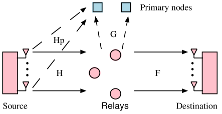
Figure 1: System model.

The source communicates with the destination via two hops, which in general lowers the required transmit power and thus reduces the interference on the primary. In the first hop, the source sends $M$ independent data streams across $M$ antennas with equal power. The relay $i$ receives

$$r_{i}=\sqrt{\frac{P_{s}}{M}}\mathbf{h}_{i}^{t}\,\mathbf{s}+n_{i},$$ (1)

where $P_{s}$ is the source transmit power, which must be less than a power constraint $\bar{P_{s}}$, $\mathbf{s}\in\mathcal{C}^{M\times 1}$ is i.i.d. Gaussian signals, $\mathbf{h}_{i}^{t}\in\mathcal{C}^{1\times M}$ is the row $i$ of $\mathbf{H}$, namely the channel vector between the relay $i$ and the source, and $n_{i}$ is additive noise with distribution $\mathcal{CN}(0,1)$.

In the second hop, a subset of the relays is selected to transmit to the destination. We define a random variable $T_{i}$ to indicate whether the relay $i$ is selected (eligible):

$$T_{i}=\left\{\begin{array}[c]{ll}1,&\mbox{the relay $i$ is eligible}\\ 0,&\mbox{otherwise}\end{array}\right..$$ (2)

No cooperation among the relays is allowed due to their distributed nature. Each relay rotates and scales $r_{i}$ by

$$c_{i}=e^{j\theta_{i}}\sqrt{\frac{P_{r}}{\mathbb{E}[T_{i}](P_{s}\sigma_{s}^{2}+1)}}.$$ (3)

where $P_{r}$ is the average relay power and $\theta_{i}$ is the rotation angle, which are designed in the sequel. Therefore, the signal transmitted by the relay $i$ is $T_{i}c_{i}\,r_{i}.$

After the relay forwarding, the received signal vector at the destination is

$$\mathbf{y} =\sqrt{\frac{P_{s}}{M}}\underset{\tilde{\mathbf{H}}}{\underbrace{\mathbf{F}\mathbf{D}\mathbf{H}}}\mathbf{s}+\underset{\tilde{\mathbf{w}}}{\underbrace{\mathbf{F}\mathbf{D}\mathbf{n}+\mathbf{w}}},$$ (4)

where $\mathbf{D}=\text{diag}(T_{1}c_{1},\cdots,T_{n}c_{n})$ is the relay processing matrix and $\tilde{\mathbf{w}}$ is the equivalent additive noise. The equivalent channel matrix $\tilde{\mathbf{H}}$ has entries

$$\big{[}\tilde{\mathbf{H}}]_{mq}=\sum_{i=1}^{n}T_{i}\,c_{i}\,f_{mi}\,h_{iq},$$ (5)

where $f_{mi}$ and $h_{iq}$ are $[\mathbf{F}]_{mi}$ and $[\mathbf{H}]_{iq}$, respectively.

In this paper, we focus on the effect of the number of relays on the secondary rate, i.e., the so-called “scaling laws” for the relays in a spectrum-sharing system. Thus, we allow $n$ to increase while $N_{p}$ remains bounded. Analysis of scaling laws has a long and established history in wireless communications. Among the many examples we mention a few, e.g., [20, 21, 14].

We refer to cross channels between secondary transmitters and primary receivers as interference links. We assume the destination knows $\mathbf{F}$, $\mathbf{D}$ and $\mathbf{H}$, and the relays only know the instantaneous channel gains to which they directly connect, i.e., $\mathbf{h}_{i}$ and the column $i$ of $\mathbf{F}$. The interference (thus the channels) from the primary to the secondary is not explicitly modeled for brevity, because its impact can be absorbed into the noise term $\tilde{{\mathbf{w}}}$.

The cross-channel CSI requirements in a TDD system can be met by the secondary nodes detecting packets emitted from the primary nodes. Otherwise, under the spectrum leasing model [22], the primary nodes can be expected to actively promote spectrum reuse by transmitting pilots that can be used for cross-channel gain estimation. The latter model applies to both TDD and FDD. Regarding the precision of cross-channel CSI, only the magnitude of the channel gains are needed, and the system can be made robust to imperfections in the cross-channel CSI to the relays, as shown in subsequent discussions (see Remark 1).

III Spectrum-Sharing with relay selection and clustering

Relays that have weak interference links but strong secondary links are useful for spectrum sharing, while relays that produce a strong interference on the primary may do more harm than good. Therefore we use relay selection. In spectrum sharing, relay selection and allocation of transmit powers are coupled through the interference constraint, an issue that is not encountered in conventional (non-spectrum sharing) relaying. To make the problem tractable, we propose a two-step approach: first the allowable interference per relay is bounded, leading to the creation of an eligible relay set. Then the secondary rate is maximized by selecting appropriate relays from among the eligible set and coordinating their transmissions in a manner shown in the sequel.

III-A Eligible Relay Selection

The interference on the primary nodes is controlled by activating only the relays with weak interference links. We design the relay selection in a distributed manner that does not require CSI exchange among the relays. A relay is eligible if and only if all of its own interference link gains are less than a pre-designed threshold $\alpha$. So from (2)

$$T_{i}=\left\{\begin{array}[c]{ll}1,\quad|g_{\ell i}|^{2}\leq\alpha\ \text{for}\ \ell=1,\cdots,N_{p}\\ 0,\quad\text{otherwise}\end{array}\right.,$$ (6)

where $|g_{\ell i}|^{2}$ is the channel gain between the relay $i$ and the primary node $\ell$. Note that $\{|g_{\ell i}|^{2}\}_{\ell,i}$ are i.i.d. exponentials with mean $\sigma_{p}^{2}$, so $\{T_{i}\}_{i}$ are i.i.d. Bernoulli random variables with success probability

$$p=(1-e^{-\alpha/\sigma_{p}^{2}})^{N_{p}}.$$ (7)

Since each relay determines eligibility based on its own interference links, the eligible relay selection is independent across the relays. The average interference from the secondary system to the primary node $\ell$ is

$$\gamma_{\ell} =\frac{1}{2}\mathbb{E}\big{[}(\sum_{i=1}^{n}g_{\ell i}t_{i})(\sum_{i=1}^{n}g_{\ell i}^{*}t_{i}^{*})\big{]}+\frac{P_{s}}{2M}\mathbb{E}\big{[}|\mathbf{h}_{p,\ell}|^{2}\big{]}$$ (8)

$$\ =\frac{P_{r}}{2}\,\sum_{i=1}^{n}\mathbb{E}\big{[}|g_{\ell i}|^{2}\big{|}T_{i}=1\big{]}+\frac{\sigma_{sp}^{2}P_{s}}{2},$$ (9)

where the factor $\frac{1}{2}$ is due to the fact that the relays and the source only transmit during half of the time. The second equality holds since the design of $\theta_{i}$ is independent of interference links, as shown soon. Since $T_{i}=1$ implies $|g_{\ell i}|^{2}\leq\alpha$ $\forall\ell$, we have

$$\mathbb{E}\big{[}|g_{\ell i}|^{2}\big{|}T_{i}=1\big{]} <\int_{0}^{\alpha}\frac{xe^{-x/\sigma_{p}^{2}}}{\sigma_{p}^{2}}dx=\sigma_{p}^{2}-e^{-\alpha/\sigma_{p}^{2}}(\alpha+\sigma_{p}^{2})$$ (10)

$$\stackrel{{\scriptstyle\Delta}}{{=}}f(\alpha).$$ (11)

Combining (9) and (11), we have $\forall\ell$, $\gamma_{\ell}\leq\gamma$ if $\alpha$ and $P_{r}$ satisfy

$$nP_{r}f(\alpha)\leq\max(\gamma_{r},0),$$ (12)

where $\gamma_{r}=2\gamma-\sigma_{sp}^{2}P_{s}$. As long as (12) holds, the interference on all the primary nodes is ensured to be less than $\gamma$, although the relays are selected distributedly. In our two-hop communication the source power $P_{s}$ is chosen so that $\gamma_{r}>0$, and otherwise the secondary rate is zero.

Remark 1

We briefly discuss CSI uncertainty in the CSI of relay cross-channel gains. Denote the (relay) estimated cross channel gain as $|\hat{g}_{\ell i}|^{2}$. For simplicity, consider $|\hat{g}_{\ell i}|^{2}$ has the same exponential distribution as the true channel gain $|g_{\ell i}|^{2}$. Assume uncertainty can be modeled as an interval, e.g., that the true cross-channel gain is in the interval $[0,(1+\epsilon)|\hat{g}_{\ell i}|^{2}]$ for some known and fixed $\epsilon$. In this case, if $\alpha$ and $P_{r}$ satisfy

$$nP_{r}f(\alpha+\epsilon)\leq\max(\gamma_{r},0),$$

the interference constraints on the primary will still be ensured. Since $f(\cdot)$ is an increasing and bounded function, the impact of uncertainty $\epsilon$ is to reduce the transmit power at the relays.

III-B Distributed Relay Clustering

The second part of the proposed method aims to maximize the secondary rate. Recall that the source and destination have $M$ antennas each; the relays are divided correspondingly into $M$ groups $\{\mathcal{G}_{m}\;,\;1\leq m\leq M\}$, where each group of relays aims to provide a virtual pipe between one of the source antennas and the corresponding destination antenna. This channel-diagonalization approach is reminiscent of [14] but requires more sophisticated analysis because the (eligible) relay set is random, as shown in the sequel.

The relay $i\in\mathcal{G}_{m}$ rotates the received signal by $\theta_{i}$ such that

$$e^{j\theta_{i}}f_{mi}h_{im}=|f_{mi}||h_{im}|.$$ (13)

In this case, all the relays in $\mathcal{G}_{m}$ forward the signal sent by the source-antenna $m$ coherently to the destination-antenna $m$.

Now, the challenge is to decide the assignment of relays to the group $\mathcal{G}_{m}$, for $1\leq m\leq M$. We focus on distributed methods so that the coordination among relays is reduced. In addition, we decouple the relay clustering from the relay selection: the relays decide their groups according to their source-relay and relay-destination channels but independent of the interference links. Therefore, under this framework, $\{\theta_{i}\}_{i=1}^{n}$ and $\{T_{i}\}_{i=1}^{n}$ are mutually independent. This decoupling allows us to leverage existing relaying methods to enhance the secondary rate while bounding the primary interference. It also greatly simplifies the analysis.

We shall consider two clustering schemes:

III-B1 Fixed Clustering

Here, each of the groups has $n/M$ relays. Subject to this condition, the relays are assigned to the groups in a pre-defined manner. Without loss of generality, we assume:

$$\mathcal{G}_{m}=\bigg{\{}i:\frac{(m-1)n}{M}+1\leq i\leq\frac{mn}{M},\;1\leq m\leq M.\bigg{\}}.$$

III-B2 Gain Clustering

In this clustering we have

$$\mathcal{G}_{m}=\bigg{\{}i:|h_{im}|>|h_{iq}|,\;\ q\neq m,\,1\leq q\leq M\bigg{\}}.$$

In other words, the groups are assigned based on the relays’ channel gain to source antennas. A relay (distributedly) decides to join in the group $m$ if its gain to the $m$-th source antenna is the stronger than any other channel gains. The group assignment of relays is independent from each other and is also independent of relay eligibility. Note that $\mathcal{G}_{m}$ is no longer fixed but depends on the source-relay channels. Because all channels are i.i.d., a relay has equal probability of choosing any of the groups. Therefore $|\mathcal{G}_{m}|$ (the cardinality of $\mathcal{G}_{m}$) is binomially distributed with parameters $(n,\frac{1}{M})$.

IV Secondary Rate in Spectrum-sharing with Relays

We first derive a general closed-form expression for the secondary rate under the proposed framework, and then evaluate the achievable rate for specific methods.

IV-A Calculation of Secondary Rate

From (4), conditioned on $\mathbf{F}$, $\mathbf{D}$ and $\mathbf{H}$, $\tilde{\mathbf{w}}$ is a Gaussian vector with autocorrelation

$$\mathbf{W}={\mathbf{I}}+\mathbf{F}\mathbf{D}\mathbf{D}^{{\dagger}}\mathbf{F}^{{\dagger}}.$$ (14)

The secondary rate in the presence of $n$ relays is denoted with $R_{n}$ and is given by:

$$R_{n}=\frac{1}{2}\log\text{det}\bigg{(}{\mathbf{I}}+\frac{P_{s}}{M}\tilde{\mathbf{H}}\tilde{\mathbf{H}}^{{\dagger}}\mathbf{W}^{-1}\bigg{)},$$ (15)

where $\frac{1}{2}$ is due to the half-duplex relay constraint.

Now, we find $R_{n}$ for large $n$. First, from (5) and (13), the entry of $\tilde{\mathbf{H}}$ is

$$\big{[}\tilde{\mathbf{H}}]_{mq} =\left\{\begin{array}[c]{ll}A_{mm}+B_{mm},&\mbox{$q=m$}\\ C_{mq},&\mbox{$q\neq m$}\end{array}\right.,$$ (18)

where

$$A_{mm} =\sqrt{\frac{P_{r}}{p(\sigma_{s}^{2}P_{s}+1)}}\sum_{i\in\mathcal{G}_{m}}T_{i}\,|f_{mi}|\,|h_{im}|,$$

$$B_{mm} =\sqrt{\frac{P_{r}}{p(\sigma_{s}^{2}P_{s}+1)}}\sum_{i\notin\mathcal{G}_{m}}T_{i}\,f_{mi}\,h_{im}\,e^{j\theta_{i}},$$

$$C_{mq} =\sqrt{\frac{P_{r}}{p(\sigma_{s}^{2}P_{s}+1)}}\sum_{i=1}^{n}T_{i}\,f_{mi}\,h_{iq}\,e^{j\theta_{i}}.$$ (19)

The terms in $A_{mm}$, $B_{mm}$ and $C_{mq}$ are mutually independent, because $\{T_{i}\}_{i=1}^{n}$ and $\{\theta_{i}\}_{i=1}^{n}$ are independent from each other. So we have the following lemma.

Lemma 1

If $\min_{1\leq m\leq M}|\mathcal{G}_{m}|\stackrel{{\scriptstyle w.p.1}}{{\longrightarrow}}\infty$ as $n\rightarrow\infty$, we have

$$\frac{A_{mm}}{n}-\frac{1}{n}\sqrt{\frac{pP_{r}}{\sigma_{s}^{2}P_{s}+1}}\sum_{i\in\mathcal{G}_{m}}\mathbb{E}[|f_{mi}||h_{im}|] \stackrel{{\scriptstyle w.p.1}}{{\longrightarrow}}0,$$ (20)

$$\frac{B_{mm}}{n}-\frac{1}{n}\sqrt{\frac{pP_{r}}{\sigma_{s}^{2}P_{s}+1}}\sum_{i\notin\mathcal{G}_{m}}\mathbb{E}[f_{mi}h_{im}e^{-j\theta_{i}}] \stackrel{{\scriptstyle w.p.1}}{{\longrightarrow}}0,$$ (21)

$$\frac{C_{mq}}{n}-\frac{1}{n}\sqrt{\frac{pP_{r}}{\sigma_{s}^{2}P_{s}+1}}\sum_{i=1}^{n}\mathbb{E}[f_{mi}h_{iq}e^{-j\theta_{i}}] \stackrel{{\scriptstyle w.p.1}}{{\longrightarrow}}0.$$ (22)

Proof:

The proof follows from [23, Theorem 2.1] and [24, Theorem 1.8.D], and is omitted here. ∎

From Lemma 1, given $|\mathcal{G}_{m}|\stackrel{{\scriptstyle w.p.1}}{{\longrightarrow}}\infty$ $\forall m$, we have:

$$\frac{\tilde{\mathbf{H}}}{n}-\text{diag}(a_{1},\cdots,a_{M})\stackrel{{\scriptstyle w.p.1}}{{\longrightarrow}}0,$$ (23)

where

$$a_{m}=\frac{1}{n}\sqrt{\frac{pP_{r}}{(\sigma_{s}^{2}P_{s}+1)}}\sum_{i\in\mathcal{G}_{m}}\mathbb{E}[|f_{mi}||h_{im}|].$$ (24)

The above analysis indicates that $\tilde{\mathbf{H}}$ converges to a diagonal matrix for large $n$ (with probability 1). We now show that $\mathbf{W}$ is also diagonalized as $n$ increases. From (14), we have

$$\big{[}\mathbf{W}\big{]}_{mq}=\sum_{i=1}^{n}\frac{T_{i}P_{r}f_{mi}f_{iq}^{*}}{p(P_{s}\sigma_{s}^{2}+1)}+\delta_{mq},$$ (25)

where $\delta_{mq}=1$ if $m=q$ and $\delta_{mq}=0$ if $m\neq q$. One can verify Kolmogorov conditions [24, Theorem 1.8.D], and therefore obtain

$$\frac{\big{[}\mathbf{W}\big{]}_{mq}}{n}-\frac{1}{n}\bigg{(}\sum_{i=1}^{n}\frac{P_{r}\mathbb{E}[f_{mi}f_{iq}^{*}]}{P_{s}\sigma_{s}^{2}+1}+\delta_{mq}\bigg{)} \stackrel{{\scriptstyle w.p.1}}{{\longrightarrow}}0,$$ (26)

where

$$\mathbb{E}[f_{mi}f_{iq}^{*}]=\left\{\begin{array}[c]{ll}\mathbb{E}[|f_{mi}|^{2}],&\mbox{$m=q$ }\\ 0,&\mbox{$m\neq q$}\end{array}\right..$$ (27)

Therefore, we have

$$\frac{\mathbf{W}}{n}-\text{diag}(b_{1},\cdots,b_{M})\stackrel{{\scriptstyle w.p.1}}{{\longrightarrow}}0,$$ (28)

where

$$b_{m}=\frac{P_{r}\sum_{i=1}^{n}\mathbb{E}[|f_{mi}|^{2}]}{n(P_{s}\sigma_{s}^{2}+1)}+\frac{1}{n}.$$ (29)

From (23) and (28), for large $n$, the end-to-end channel between the source and the destination is approximately decoupled into $M$ parallel channels under the proposed framework, where the channel coefficient $m$ is $a_{m}$ and the received noise has variance $b_{m}$. The capacity of this parallel channel is

$$\overline{R}=\frac{1}{2}\sum_{m=1}^{M}\log\big{(}1+\frac{nP_{s}a_{m}^{2}}{Mb_{m}}\big{)},$$ (30)

Therefore, it is reasonable to expect that $R_{n}\approx\overline{R}$ for large $n$. After some calculation (omitted for brevity), we obtain the following result.

Theorem 1

Consider a secondary system with an $M$-antenna source, an $M$-antenna destination, and $n$ single-antenna relays, in the presence of $N$ primary nodes each tolerating interference no more than $\gamma$. The secondary rate satisfies

$$R_{n}-\overline{R}\stackrel{{\scriptstyle w.p.1}}{{\longrightarrow}}0,\quad n\rightarrow\infty,$$ (31)

under the proposed relay selection and clustering framework.

IV-B Achievable Rate under Specific Clustering Schemes

We apply Theorem 1 to fixed clustering and gain clustering.

IV-B1 Fixed Clustering

In this scheme, $|\mathcal{G}_{m}|=\frac{n}{M}$ (so Lemma 1 is applicable), and $|f_{mi}|$ and $|h_{im}|$ are i.i.d. Rayleigh random variables with mean $\frac{\sigma_{d}\sqrt{\pi}}{2}$ and $\frac{\sigma_{s}\sqrt{\pi}}{2}$, respectively. Therefore, from (24), $a_{m}=\frac{\pi\sigma_{s}\sigma_{d}}{4M}\sqrt{\frac{pP_{r}}{\sigma_{s}^{2}P_{s}+1}},$ for $1\leq m\leq M$. Under this clustering, $|f_{mi}|^{2}$ is i.i.d. exponential with mean $\sigma_{d}^{2}$, and we have $b_{m}=\frac{\sigma_{d}^{2}P_{r}}{\sigma_{s}^{2}P_{s}+1}+\frac{1}{n},$ for $1\leq m\leq M$. Substituting $a_{m}$ and $b_{m}$ into (30), $\overline{R}$ becomes

$$R^{(f)}=\frac{M}{2}\log\bigg{(}1+\frac{np\pi^{2}\sigma_{s}^{2}\sigma_{d}^{2}P_{r}P_{s}}{16M^{3}(\sigma_{d}^{2}P_{r}+n^{-1}(\sigma_{s}^{2}P_{s}+1))}\bigg{)}.$$ (32)

From Theorem 1, under fixed clustering, we have: $R_{n}-R^{(f)}\stackrel{{\scriptstyle w.p.1}}{{\longrightarrow}}0.$

IV-B2 Gain Clustering

Since $|\mathcal{G}_{m}|$ is binomially distributed with parameters $(n,\frac{1}{M})$, we have $|\mathcal{G}_{m}|/n\stackrel{{\scriptstyle w.p.1}}{{\longrightarrow}}1/M$, and Lemma 1 is again applicable. Due to the independence of $|f_{mi}|$ and $|h_{im}|$, from (24), we have

$$a_{m}=\frac{1}{n}\sqrt{\frac{pP_{r}}{(\sigma_{s}^{2}P_{s}+1)}}\sum_{i\in\mathcal{G}_{m}}\mathbb{E}[|f_{mi}|]\mathbb{E}[|h_{im}|].$$ (33)

where $\mathbb{E}[|f_{mi}|]=\frac{\sigma_{d}\sqrt{\pi}}{2}$ (i.i.d. Rayleigh) and $\mathbb{E}[|h_{im}|]=\max_{1\leq m\leq M}|h_{mi}|$, which is the maximum of $M$ i.i.d. Rayleigh random variables. We have

$$\mu_{h} =\mathbb{E}\big{[}\max_{1\leq m\leq M}|h_{im}|\big{]}$$

$$=\int_{0}^{\infty}\frac{2Mx^{2}}{\sigma_{s}^{2}}e^{-x^{2}/\sigma_{s}^{2}}\big{(}1-e^{-x^{2}/\sigma_{s}^{2}}\big{)}^{M-1}\,dx$$ (34)

$$=\sum_{m=0}^{M-1}(-1)^{M-m-1}\big{(}_{\ \ m}^{M-1}\big{)}\frac{\sigma_{s}M\Gamma(\frac{3}{2})}{(M-m)^{3/2}}.$$ (35)

Note that $\mu_{h}=\frac{\sigma_{s}\sqrt{\pi}}{2}$ for $M=1$ (no selection is needed), which is identical to the fixed clustering. Based on (33) and $|\mathcal{G}_{m}|/n\stackrel{{\scriptstyle w.p.1}}{{\rightarrow}}1/M$, we have $a_{m}-\frac{\sigma_{d}\mu_{h}}{2M}\sqrt{\frac{p\pi P_{r}}{(\sigma_{s}^{2}P_{s}+1)}}\stackrel{{\scriptstyle w.p.1}}{{\longrightarrow}}0.$

Under this clustering, $b_{m}$ remains the same as the fixed clustering case, since $|f_{mi}|$ is still i.i.d. Rayleigh for $i\in\mathcal{G}_{m}$, $\forall m$. Substituting $a_{m}$ and $b_{m}$ into (30), we have

$$R^{(g)}=\frac{M}{2}\log\bigg{(}1+\frac{np\pi\mu_{h}^{2}\sigma_{d}^{2}P_{r}P_{s}}{4M^{3}(\sigma_{d}^{2}P_{r}+n^{-1}(\sigma_{s}^{2}P_{s}+1))}\bigg{)},$$ (36)

then: $R_{n}-R^{(g)}\stackrel{{\scriptstyle w.p.1}}{{\longrightarrow}}0.$

V Optimal Power Strategy for Spectrum-sharing with relays

In general, one may envision two competing philosophies for relay selection: (1) Allow only relays that have extremely weak interference links to the primary. Only very few relays will qualify but each of them can transmit at high power. (2) Allow a large number of relays to be activated. In this case the relay powers must be lowered because not all interference links are as “good” as the previous case.

The key question is: which approach is better? Should we use a few select relays with excellent interference profiles, or more relays operating at lower power? In this section, we optimize the threshold $\alpha$, the relay power $P_{r}$ and the source power $P_{s}$, while bounding the primary interference. The results of this section show that in general the balance tips in favor of having more eligible relays operating at low power.

V-A Optimal Design of $\alpha$ and $P_{r}$

Consider a fixed $P_{s}$. Since $\alpha$ and $P_{r}$ depend on each other via (12), given $\alpha$ the maximum $P_{r}$ is

$$P_{r}=\frac{\gamma_{r}}{nf(\alpha)}.$$ (37)

Substituting (37) and (7) into (32) and (36) shows that $R^{(f)}$ and $R^{(g)}$ attain their maxima (as a function of $\alpha$) at $\alpha=\alpha_{0}$ where:

$$\alpha_{o}=\arg\max_{\alpha}\frac{\gamma_{r}P_{s}(1-e^{-\alpha/\sigma_{p}^{2}})^{N_{p}}}{\gamma_{r}\sigma_{d}^{2}+(\sigma_{s}^{2}P_{s}+1)f(\alpha)}.$$ (38)

A closed-form solution for $\alpha_{o}$ is unavailable but numerical solution can be easily obtained. Figure 2 shows the optimal design of $\alpha$ based on (38). For both fixed clustering and gain clustering, according to (38), $\alpha_{o}=1.7$ maximizes the secondary rate.

Now, we characterize the asymptotic behavior of $\alpha_{o}$, equivalently the optimal $P_{r}$. Because (38) is independent of $n$, the optimal threshold $\alpha$ is not a function of $n$. So from (37) the optimal average transmit power is $P_{r}=\Theta(n^{-1})$, i.e., there exist real constants $d_{1},d_{2}>0$ so that $d_{1}n^{-1}\leq P_{r}\leq d_{2}n^{-1}$. This implies that the secondary system should on average allow many relays to operate at low power. One may intuitively interpret this result as follows. To comply with the primary interference constraints, the sum power of relays must be bounded, and by spreading the total power among more relays better beamforming gain is achieved via coherent transmission.

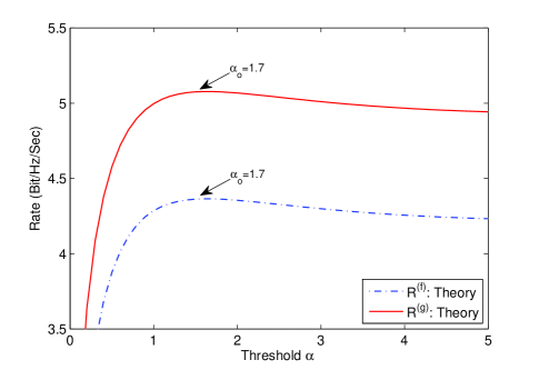
Figure 2: Optimal value of selection threshold $\alpha$ under $P_{s}=5,n=100$

Now, we study the scaling of the secondary rate. Consider examples with fixed clustering (Eq. (32)) and gain clustering (Eq. (36)). If $P_{r}=\Theta(n^{-1})$, for fixed $\alpha$ (not necessarily optimal), we have

$$R^{(f)}=\frac{M}{2}\log n+C_{1},\quad R^{(g)}=\frac{M}{2}\log n+C_{1}+C_{2},$$ (39)

where

$$C_{1}=\frac{M}{2}\log\frac{p\pi^{2}\sigma_{s}^{2}\sigma_{d}^{2}\gamma_{r}P_{s}}{16M^{3}(\sigma_{s}^{2}P_{s}+1)(\sigma_{p}^{2}\gamma_{r}+f(\alpha))}$$

and $C_{2}=\log\frac{4\mu_{h}^{2}}{\pi\sigma_{s}^{2}}$. One can view $C_{2}$ as multi-antenna diversity gain by selecting over source-relay channels. From (39), the secondary rate increases as $(M\log n)/2$, which is summarized in the next theorem.

Theorem 2

Consider a secondary system with an $M$-antenna source, an $M$-antenna destination, and $n$ single-antenna relays, in the presence of $N$ primary nodes each tolerating interference no more than $\gamma$. For $P_{r}=\Theta(n^{-1})$ and fixed $\alpha$, the secondary rate satisfies

$$\frac{R_{n}}{\frac{M}{2}\log n}\stackrel{{\scriptstyle w.p.1}}{{\longrightarrow}}1,$$ (40)

under the proposed framework with both fixed clustering and gain clustering.

Theorem 2 holds for a broad class of clustering schemes, as long as the corresponding $a_{m}$ and $b_{m}$ are bounded but non-zero, i.e., the secondary end-to-end equivalent channel is diagonalized with probability 1 as $n$ grows.

Remark 2

It is possible to extend our results to the case of peak interference constraint $\gamma$. The secondary source will manage its instantaneous interference to be smaller than $\gamma_{s}$ on all primary nodes by adjusting its transmit power according to the largest cross-channel gain to the primaries. Then, the sum interference from all the relays must be smaller than $\gamma_{r}=\gamma-\gamma_{s}$. Let $P_{r}=\xi/n$ where $\xi$ is a positive constant. The instantaneous interference from all the relays to the primary node $\ell$ is $\gamma_{\ell}=\xi\sum_{i=1}^{n}T_{i}|g_{\ell i}|^{2}/n$. This implies that

$$\gamma_{\ell}-\xi\;\mathbb{E}[T_{i}\;|g_{\ell i}|^{2}]\stackrel{{\scriptstyle w.p.1}}{{\longrightarrow}}1$$

for an arbitrary $i\in\{1,\ldots,n\}$, where we have used the fact that $T_{i}$ and $g_{\ell i}$ for all $i$ have identical distributions. Therefore, $\xi=\gamma_{r}\big{(}\mathbb{E}[T_{i}\;|g_{\ell i}|^{2}]\big{)}^{-1}$ ensures the instantaneous interference on all the primary nodes to be smaller than $\gamma$ with probability $1$.

V-B Optimal Source Power

Due to the primary interference constraints, for any chosen $\alpha$ the higher the source power $P_{s}$, the lower the relay power $P_{r}$, and vice versa. From (32) and (36), the rate-maximizing $P_{s}$ is

$$P_{s}^{*}=\arg\max_{0<P_{s}<\min(\bar{P_{s}},2\gamma)}\frac{(2\gamma-\sigma_{sp}^{2}P_{s})P_{s}}{(2\gamma-\sigma_{sp}^{2}P_{s})\sigma_{d}^{2}+(\sigma_{s}^{2}P_{s}+1)f(\alpha)}.$$ (41)

The unique solution of the above optimization problem is

$$P_{s}^{*}=\min(P_{o},\bar{P_{s}}),$$ (42)

where $P_{0}=\frac{\gamma}{\sigma_{sp}^{2}}$ if $\sigma_{sp}^{2}\sigma_{d}^{2}=\sigma_{s}^{2}f(\alpha)$, otherwise:

$$P_{o}= \frac{2\gamma\sigma_{d}^{2}}{\sigma_{sp}^{2}\sigma_{d}^{2}-\sigma_{s}^{2}f(\alpha)}$$

$$-\frac{\sqrt{\big{(}2\gamma\sigma_{d}^{2}f(\alpha)+f^{2}(\alpha)\big{)}\big{(}\sigma_{sp}^{2}+2\gamma\sigma_{s}^{2}\big{)}}}{\sigma_{sp}\big{(}\sigma_{sp}^{2}\sigma_{d}^{2}-\sigma_{s}^{2}f(\alpha)\big{)}}$$ (43)

Figure 3 demonstrates the optimal source power as a function of three channel parameters $\sigma_{sp}^{2}$, $\sigma_{s}^{2}$ and $\sigma_{d}^{2}$. Three curves are shown, in each case one parameter varies while the other two are held constant (at unity). In this Figure $\bar{P_{s}}=10$, $\gamma=5$ and $f(\alpha)=0.8$. As the source-primary channels become stronger, the source needs to reduce power; otherwise, the relay power must decrease to comply with the primary interference constraints, which curbs the rate achieved by the second hop. If the source-relay channels become stronger, the relay-destination links is the bottleneck and the relays need to transmit at higher power, thus once again the source needs to reduce power. In contrast, when the relay-destination channels become better, the source-relay channels are the bottleneck so the source needs to increase power.

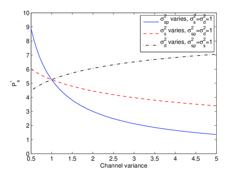
Figure 3: Optimal source power with $\gamma=5,f(\alpha)=0.8$

V-C Asymptotic Reduction of Interference on Primary

Multiple relays produce opportunities not only to enhance the secondary rate but also to reduce the interference on the primary. Suppose the interference on the primary nodes to be bounded as $\gamma=O\big{(}n^{-\delta}\big{)},$ which goes to zero as $n\rightarrow\infty$. From (12), it is sufficient to comply with this constraint if $P_{r}$ decreases as $\Theta(n^{-(1+\delta)})$ and $P_{s}$ decreases as $\Theta(n^{-\delta})$. Substituting $P_{r}$ and $P_{s}$ into the expression of $R^{(f)}$ given by (32) and following some order calculation (the analysis of $R^{(g)}$ is the same thus omitted), we have

$$R^{(f)}=\left\{\begin{array}[c]{ll}\frac{M(1-2\delta)}{2}\log n+O(1)&\mbox{$\delta<\frac{1}{2}$}\\ O(1)&\mbox{$\delta\geq\frac{1}{2}$}\end{array}\right.$$ (44)

The above equation characterizes the trade-off between the secondary rate and the interference on the primary: the faster of the interference reduction, the slower of the rate growth. It also shows that the interference on the primary nodes may be mitigated (to zero asymptotically), while the secondary rate maintains to increase as $\Theta(\log n)$.

Remark 3

In the above, the allowable interference $\gamma$ is made to decline as $\Theta(n^{-\delta})$, which leads the growth rate to decrease linearly in $\delta$. If $\gamma$ is reduced more slowly, e.g., decreasing as $\Theta(\frac{1}{\log n})$, the secondary rate can increase at a rate of $\frac{M}{2}\log n$. If we try to mitigate the primary interference faster than $\Theta(1/\sqrt{n})$, the secondary rate will not increase logarithmically with $n$.

VI Spectrum-sharing with Alternating Relay Protocol

In this section we consider issues raised by the relay half-duplex constraint, i.e., limitations that arise because relays cannot listen to the source at the same time as they are transmitting. When a subset of relays are activated for relaying the previously received information, the inactive relays are able to listen and receive information from the source, thus in principle the source can transmit continually and the half-duplex loss can be mitigated. This is the basic idea of spectrum sharing with Alternating Relay Protocol, which is the subject of this section.

The protocol consists of $L$ transmission frames, as shown in Figure 4. It is assumed the channel coefficient remains constant during each frame, but varies independently from frame to frame. The source transmits during frames $1$ through $L-1$, and remains silent during frame $L$. Since the source transmits $L-1$ data segments during $L$ time intervals, the rate loss induced by the half-duplex relaying is a factor of $\frac{L-1}{L}$. The relays are partitioned into two groups $\mathcal{G}_{1}=\{1\leq i\leq\frac{n}{2}\}$ and $\mathcal{G}_{2}=\{\frac{n}{2}+1\leq i\leq n\}$. During even-numbered transmission frames a subset of the relays in $\mathcal{G}_{1}$ transmit to the destination, while the relays in $\mathcal{G}_{2}$ listen to the source. During odd-numbered transmission frames, a subset of the relays in $\mathcal{G}_{2}$ transmit, while the relays in $\mathcal{G}_{1}$ listen. As shown later, each of the two relay groups asymptotically achieves a rate that grows as $\frac{M}{2}\frac{L-1}{L}\log n$, thus the overall system has a rate that grows proportionally to $M\frac{L-1}{L}\log n$. Therefore a good part of the half-duplex rate loss can be recovered.

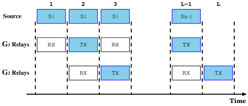
Figure 4: Transmission schedule in the alternating relay protocol (ARP)

When either group $\mathcal{G}_{1}$ or group $\mathcal{G}_{2}$ is in the transmit mode, a subset of relays in the corresponding group is selected to transmit. A relay is selected (eligible) if its interference links satisfy (6), similar to Section III-A. The average interference power on the primary node $\ell$ takes slightly different forms depending on whether $L$ is even or odd. When $L$ is even:

$$\gamma_{\ell}= \frac{(L-1)\sigma_{sp}^{2}P_{s}}{L}+\frac{P_{r}}{2}\sum_{i\in\mathcal{G}_{1}}\mathbb{E}\big{[}|g_{\ell i}|^{2}\big{|}T_{i}=1\big{]}$$

$$\qquad+\frac{(L-2)P_{r}}{2L}\sum_{i\in\mathcal{G}_{2}}\mathbb{E}\big{[}|g_{\ell i}|^{2}\big{|}T_{i}=1\big{]},$$ (45)

and when $L$ is odd:

$$\gamma_{\ell}= \frac{(L-1)\sigma_{sp}^{2}P_{s}}{L}+\frac{(L-1)P_{r}}{2L}\bigg{(}\sum_{i\in\mathcal{G}_{1}}\mathbb{E}\big{[}|g_{\ell i}|^{2}\big{|}T_{i}=1\big{]}$$

$$\qquad+\sum_{i\in\mathcal{G}_{2}}\mathbb{E}\big{[}|g_{\ell i}|^{2}\big{|}T_{i}=1\big{]}\bigg{)}\;.$$ (46)

To comply with the interference constraints on the primary nodes, the threshold $\alpha$ and the relay power $P_{r}$ shall satisfy

$$nP_{r}f(\alpha)\leq\max(\gamma_{L},0),$$ (47)

where $\gamma_{L}=\frac{2L}{L-1}\gamma-2\sigma_{sp}^{2}P_{s}$ with $P_{s}$ so that $\gamma_{L}>0$, and we use the fact that $\mathbb{E}\big{[}|g_{\ell i}|^{2}\big{|}T_{i}=1\big{]}=f(\alpha)$. Since from Section V the optimal $P_{r}$ is proportional to $n^{-1}$, we let $P_{r}=\eta/n$, and re-write (47) as

$$\eta f(\alpha)\leq\max(\gamma_{L},0).$$ (48)

For the Alternating Relay Protocol, relay clustering is accomplished in a manner similar to Section III-B, therefore the details are omitted. During frame $2k$ (or $2k+1$), let $\mathcal{G}_{m,k}^{(1)}\subset\mathcal{G}_{1}$ (or $\mathcal{G}_{m,k}^{(2)}\subset\mathcal{G}_{2}$) be the set of relays that assists the antenna pair $m$. As long as $\min_{m,k,d}|\mathcal{G}_{m,k}^{(d)}|\rightarrow\infty$, the secondary rate will be obtained following the analysis similar to Section IV.

Remark 4

At any point in time, it is possible to allow all non-transmitting relays to listen to the source, and be eligible to transmit in the next frame. This may give some gains, however, it also complicates the relay selection by introducing dependence between not only interference links but also other links such as source-relay and relay-relay links. It may be better for a relay even with a small interference on primary to remain inactive if it has also a weak channel to destination (therefore it cannot help much) but has a strong channel to the source (therefore it can listen well for the next round). Thus, any gains will come with a loss of elegance and tractability, and therefore this approach is not considered in this paper.

VI-A A Simple Example: $L=3$

For illustration purposes, we consider $L=3$, where $\mathcal{G}_{1}$ ($\mathcal{G}_{2}$) listen to the source during frame $1$, and then transmit to the destination during frame $2$ (frame $3$). We assume fixed clustering is used with $|\mathcal{G}_{m,1}^{(d)}|=n/(2M)$, for $1\leq m\leq M$ and $1\leq d\leq 2$. Let $\mathbf{H}_{d}$ ($\mathbf{F}_{d}$) be the channel coefficient matrix between the relays in $\mathcal{G}_{d}$ and the source (the destination), and $\mathbf{H}_{r}$ be the channel coefficient matrix between $\mathcal{G}_{1}$ and $\mathcal{G}_{2}$ with i.i.d. $\mathcal{CN}(0,\sigma_{r}^{2})$ entries.

We now analyze the rate achieved under Alternating Relay Protocol. The optimization of the threshold and the source power follows in a manner similar to Section V and thus is omitted here.

VI-A1 Rate Achieved by $\mathcal{G}_{1}$

After listening to the source at frame $1$, $\mathcal{G}_{1}$ relays to the destination at frame $2$. At the end of frame $2$, similar to (4) the received signal at the destination is

$$\mathbf{y}_{1} =\sqrt{\frac{P_{s}}{M}}\underset{\tilde{\mathbf{H}}_{1}}{\underbrace{\mathbf{F}_{1}\mathbf{D}_{1}\mathbf{H}_{1}}}\mathbf{s}_{1}+\underset{\tilde{\mathbf{w}}_{1}}{\underbrace{\mathbf{F}_{1}\mathbf{D}_{1}\mathbf{n}_{1}+\mathbf{w}_{1}}},$$ (49)

where $\mathbf{s}_{1}$ is the signal sent by the source during frame $1$, $\mathbf{n}_{1}$ is the noise forwarded by the group $\mathcal{G}_{1}$ of relays, $\mathbf{w}_{1}$ is the destination noise. For the group $\mathcal{G}_{1}$ the relay gains are collected into the relay processing matrix

$$\mathbf{D}_{1}=\text{diag}(T_{1}c_{1},\cdots,T_{\frac{n}{2}}c_{\frac{n}{2}}),$$ (50)

where $c_{i}$ is given by (3) so that the average relay power constraints are satisfied. One can verify that the equivalent channel $\tilde{\mathbf{H}}_{1}$

$$\frac{\tilde{\mathbf{H}}_{1}}{\sqrt{n}}\stackrel{{\scriptstyle w.p.1}}{{\longrightarrow}}\rho_{1}{\mathbf{I}},$$ (51)

where $\rho_{1}=\frac{\pi\sigma_{s}\sigma_{d}}{8M}\sqrt{\frac{p\eta}{\sigma_{s}^{2}P_{s}+1}}$. The auto-covariance of equivalent noise $\tilde{\mathbf{w}}_{1}$ is

$$\frac{1}{n}\mathbf{W}_{1}\stackrel{{\scriptstyle w.p.1}}{{\longrightarrow}}\lambda_{1}{\mathbf{I}},$$ (52)

where $\lambda_{1}=\frac{\eta\sigma_{d}^{2}}{2(\sigma_{s}^{2}P_{s}+1)}+1$. Therefore, the end-to-end channel is diagonalized for large $n$, and similar to the results in Theorem 1, the rate achieved $R^{(1)}$ during frame $2$ satisfies:

$$R^{(1)}-M\log\bigg{(}1+\frac{np\pi^{2}\sigma_{s}^{2}\sigma_{d}^{2}\eta P_{s}}{32M^{3}(\eta\sigma_{d}^{2}+2\sigma_{s}^{2}P_{s}+2)}\bigg{)}\stackrel{{\scriptstyle w.p.1}}{{\longrightarrow}}0.$$ (53)

VI-A2 Rate Achieved by $\mathcal{G}_{2}$

During frame $2$, the relays in $\mathcal{G}_{2}$ receive the signal vector:

$$\mathbf{r}_{2} =\sqrt{\frac{P_{s}}{M}}\mathbf{H}_{2}\mathbf{s}_{2}+\mathbf{H}_{r}\mathbf{D}_{1}\bigg{(}\sqrt{\frac{P_{s}}{M}}\mathbf{H}_{1}\mathbf{s}_{1}+\mathbf{n}_{1}\bigg{)}+\mathbf{n}_{2},$$ (54)

where $\mathbf{s}_{2}$ is the signal sent by the source during frame $2$, and the second term corresponds to the interference from the transmission of $\mathcal{G}_{1}$. During frame $3$ the relays in $\mathcal{G}_{2}$ transmit to the destination with a processing matrix

$$\mathbf{D}_{2}=\text{diag}(T_{\frac{n}{2}+1}\,c_{\frac{n}{2}+1},\cdots,T_{n}c_{n}),$$ (55)

where, to satisfy the power constraints, for $\frac{n}{2}+1\leq i\leq n$

$$c_{i}=e^{j\theta_{i}}\sqrt{\frac{\eta}{np(P_{s}\sigma_{s}^{2}+\eta\sigma_{r}^{2}/2+1)}}.$$ (56)

At the end of frame $3$, the received signal at the destination is

$$\mathbf{y}_{2}= \mathbf{F}_{2}\mathbf{D}_{2}\mathbf{r}_{2}+\mathbf{w}_{2}$$

$$= \sqrt{\frac{P_{s}}{M}}\underset{\tilde{\mathbf{H}}_{2}}{\underbrace{\mathbf{F}_{2}\mathbf{D}_{2}\mathbf{H}_{2}}}\mathbf{s}_{2}+\sqrt{\frac{P_{s}}{M}}\mathbf{F}_{2}\mathbf{D}_{2}\mathbf{H}_{r}\mathbf{D}_{1}\mathbf{H}_{1}\mathbf{s}_{1}$$

$$+\underset{\tilde{\mathbf{w}}_{2}}{\underbrace{\mathbf{F}_{2}\mathbf{D}_{2}\mathbf{H}_{r}\mathbf{D}_{1}\mathbf{n}_{1}+\mathbf{F}_{2}\mathbf{D}_{2}\mathbf{n}_{2}+\mathbf{w}_{2}}}\quad.$$ (57)

After correctly decoding $\mathbf{s}_{1}$, the destination cancels the inter-relay interference, i.e., the second term in (57). After eliminating the inter-relay interference, we have an equivalent channel:

$$\mathbf{y}_{2}=\sqrt{\frac{P_{s}}{M}}\tilde{\mathbf{H}}_{2}\mathbf{s}_{2}+\tilde{\mathbf{w}}_{2}.$$ (58)

Following steps similar to (23) and (24), we have

$$\frac{\tilde{\mathbf{H}}_{2}}{\sqrt{n}}\stackrel{{\scriptstyle w.p.1}}{{\longrightarrow}}\rho_{2}{\mathbf{I}},$$ (59)

where $\rho_{2}=\frac{\pi\sigma_{s}\sigma_{d}}{8M}\sqrt{\frac{p\eta}{\sigma_{s}^{2}P_{s}+\eta\sigma_{r}^{2}/2+1}}$. Note that $\tilde{\mathbf{w}}_{2}$ is still a zero-mean Gaussian vector with auto-covariance

$$\frac{1}{n}\mathbf{W}_{2}=\mathbf{F}_{2}\mathbf{D}_{2}\mathbf{H}_{r}\mathbf{D}_{1}\mathbf{D}_{1}^{{\dagger}}\mathbf{H}_{r}^{{\dagger}}\mathbf{D}_{2}^{{\dagger}}\mathbf{F}_{2}^{{\dagger}}+\mathbf{F}_{2}\mathbf{D}_{2}\mathbf{D}_{2}^{{\dagger}}\mathbf{F}_{2}^{{\dagger}}+{\mathbf{I}}.$$ (60)

In the right hand side of the above equation, we have

$$\mathbf{H}_{r}\mathbf{D}_{1}\mathbf{D}_{1}^{{\dagger}}\mathbf{H}_{r}^{{\dagger}} =\frac{\eta}{np(P_{s}\sigma_{s}^{2}+1)}\mathbf{H}_{r}\,\text{diag}(T_{1},\cdots,T_{\frac{n}{2}})\,\mathbf{H}_{r}^{{\dagger}}$$

$$\stackrel{{\scriptstyle w.p.1}}{{\longrightarrow}}\frac{\eta\sigma_{r}^{2}}{2(P_{s}\sigma_{s}^{2}+1)}{\mathbf{I}}.$$ (61)

Therefore,

$$\mathbf{W}_{2}\stackrel{{\scriptstyle w.p.1}}{{\longrightarrow}}\lambda_{2}{\mathbf{I}},$$ (62)

where

$$\lambda_{2}= \frac{1}{2(P_{s}\sigma_{s}^{2}+\eta\sigma_{r}^{2}/2+1)}\bigg{[}\frac{\eta^{2}\sigma_{d}^{2}\sigma_{r}^{2}}{2(P_{s}\sigma_{s}^{2}+1)}+\eta\sigma_{d}^{2}\bigg{]}+1.$$ (63)

Combining (59) and (60) , the rate achieved by $\mathcal{G}_{2}$ is $R^{(2)}$ where

$$R^{(2)}-M\log\big{(}1+\frac{nP_{s}\rho_{2}^{2}}{M\lambda_{2}}\big{)}\stackrel{{\scriptstyle w.p.1}}{{\longrightarrow}}0.$$ (64)

The overall rate is given by the following theorem.

Theorem 3

Consider a secondary system with an $M$-antenna source, an $M$-antenna destination, and $n$ single-antenna relays, in the presence of $N$ primary nodes each tolerating interference no more than $\gamma$. The secondary rate satisfies

$$\overline{R}-\big{(}R^{(1)}+R^{(2)}\big{)}/3\stackrel{{\scriptstyle w.p.1}}{{\longrightarrow}}0,$$ (65)

under the Alternating Relaying Protocol with $L=3$ and fixed clustering.

From Theorem 3, the growth rate of $\overline{R}$ is

$$\frac{\overline{R}}{\frac{2M}{3}\log n}\stackrel{{\scriptstyle w.p.1}}{{\longrightarrow}}1.$$ (66)

Remark 5

Theorem 3 can be generalized to an arbitrary number of transmission blocks $L$. For general $L$ we can conclude:

$$\frac{\overline{R}}{\frac{(L-1)M}{L}\log n}\stackrel{{\scriptstyle w.p.1}}{{\longrightarrow}}1.$$

As $L$ increases, the growth rate of $\overline{R}$ approaches the maximum value of $M\log n$.

VII Numerical Results

Unless otherwise specified, we use parameters $\bar{P_{s}}=10$, $M=2$, $N=1$, $\gamma=5$ and $\sigma_{s}^{2}=\sigma_{d}^{2}=1$.

The secondary rates as a function of source transmit power are presented by Figure 5. The theoretical rate under various $P_{s}$ is calculated according to (32) and (36). Recall that the theoretically optimal $P_{s}$ given by (42) is obtained by (32) and (36). When the source interference links are very weak, e.g., $\sigma_{sp}^{2}=0.1$, maximizing the source power is optimal, which is similar to non-spectrum-sharing networks. When the source interference links is strong, e.g., $\sigma_{sp}^{2}=1,2$, unlike non-spectrum-sharing networks, the secondary achieves higher rate if the source transmit at power lower than the maximum value. This is because the source needs to ensure the relays can operate with sufficient power, subject to the total interference constraints on the primary nodes.

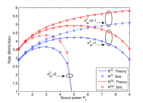
Figure 5: Throughput as a function of source power when $n=100,\sigma_{2}=\sigma_{d}=\sigma_{p}=1$

Figure 6 verifies Theorem 1 under fixed clustering and gain clustering. Here, $\alpha=\gamma$, $\sigma_{sp}^{2}=1$, $P_{r}$ is given by (37) and $P_{s}=5$, which is almost optimal as shown in Figure 5. The simulated average rate of $R_{n}$ under two clustering schemes are compared to $R^{(f)}$ given by (32) and $R^{(g)}$ given by (36), respectively, where the results are well matched for modest value of $n$. The secondary rate increases as the interference links of relays become weaker (smaller $\sigma_{p}^{2}$), since the relays can transmit at higher power (but the sum relay power is still bounded with $n$).

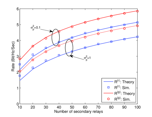
Figure 6: Secondary rate under two clustering schemes

Figure 7 illustrates the tradeoff between maximizing secondary rate and minimizing interference on the primary. The interference power is $\gamma=5(n)^{-\delta}$ with $\delta=0.1$ and $0.2$, respectively. For $\delta=0.2$, the interference power decreases faster than $\delta=0.1$, while the secondary rate increases more slowly.

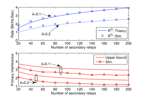
Figure 7: Secondary rate and primary interference as a function of number of relays

The rate of Alternating Relaying Protocol (Theorem 3) is shown in Figure 8. We consider $\alpha\rightarrow\infty$, where all the relays in $\mathcal{G}_{1}$ and $\mathcal{G}_{2}$ transmit alternatively. Here, $P_{s}=5$ and $P_{r}$ is determined by (47). The simulated rates match the theoretic analysis well under modest value of $n$. As the relay-relay channel becomes weaker (smaller $\sigma_{r}^{2}$), the inter-relay interference is reduced, and thus the secondary rate increases.

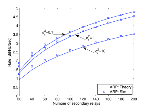
Figure 8: Secondary rate under the alternating relaying protocol

VIII Conclusion

This paper studies spectrum sharing networks with distributed AF relaying to improve the secondary rate and reduce the interference on the primary. In the asymptote of large $n$ (number of relays) the optimal power strategy for the secondary source and relays was found, achieving a secondary rate proportionally to $\log n$. The half-duplex rate loss was reduced and the scaling of secondary rate was enhanced by the introduction of the Alternating Relay Protocol. The trade-off between the secondary rate and the interference on the primary was characterized. Finally, our results show that even without cross channel information at the secondary, the secondary rate can achieve the growth rate $\log n$.

References

- [1] A. Ghasemi and E. S. Sousa, “Fundamental limits of spectrum-sharing in fading environments,” IEEE Trans. Wireless Commun., vol. 6, no. 2, pp. 649–658, Feb. 2007.
- [2] M. Gastpar, “On capacity under receive and spatial spectrum-sharing constraints,” IEEE Trans. Inform. Theory, vol. 53, no. 2, pp. 471–487, Feb. 2007.
- [3] A. Özgür, O. Lévêque, and D. Tse, “Hierarchical cooperation achieves optimal capacity scaling in ad hoc networks,” IEEE Trans. Inform. Theory, vol. 53, no. 10, pp. 3549 –3572, Oct. 2007.
- [4] Y. Liang and V. V. Veeravalli, “Cooperative relay broadcast channels,” IEEE Trans. Inform. Theory, vol. 53, no. 3, pp. 900 –928, Mar. 2007.
- [5] D. Chen, K. Azarian, and J. Laneman, “A case for amplify-forward relaying in the block-fading multiple-access channel,” IEEE Trans. Inform. Theory, vol. 54, no. 8, pp. 3728 –3733, Aug. 2008.
- [6] O. Şahin, O. Simeone, and E. Erkip, “Interference channel with an out-of-band relay,” IEEE Trans. Inform. Theory, vol. 57, no. 5, pp. 2746 –2764, May 2011.
- [7] G. Zhao, J. Ma, G. Li, T. Wu, Y. Kwon, A. Soong, and C. Yang, “Spatial spectrum holes for cognitive radio with relay-assisted directional transmission,” IEEE Trans. Wireless Commun., vol. 8, no. 10, pp. 5270 –5279, Oct. 2009.
- [8] J. Mietzner, L. Lampe, and R. Schober, “Distributed transmit power allocation for multihop cognitive-radio systems,” IEEE Trans. Wireless Commun., vol. 8, no. 10, pp. 5187 –5201, Oct. 2009.
- [9] V. Asghari and S. Aissa, “Cooperative relay communication performance under spectrum-sharing resource requirements,” in ICC, May 2010.
- [10] L. Li, X. Zhou, H. Xu, G. Li, D. Wang, and A. Soong, “Simplified relay selection and power allocation in cooperative cognitive radio systems,” IEEE Trans. Wireless Commun., vol. 10, no. 1, pp. 33 –36, Jan. 2011.
- [11] M. Naeem, D. Lee, and U. Pareek, “An efficient multiple relay selection scheme for cognitive radio systems,” in ICC, IEEE, May 2010.
- [12] Y. Zou, J. Zhu, B. Zheng, and Y.-D. Yao, “An adaptive cooperation diversity scheme with best-relay selection in cognitive radio networks,” IEEE Trans. Signal Processing, vol. 58, no. 10, pp. 5438 –5445, Oct. 2010.
- [13] J. Lee, H. Wang, J. Andrews, and D. Hong, “Outage probability of cognitive relay networks with interference constraints,” IEEE Trans. Wireless Commun., vol. 10, no. 2, pp. 390 –395, Feb. 2011.
- [14] H. Bölcskei, R. Nabar, O. Oyman, and A. Paulraj, “Capacity scaling laws in MIMO relay networks,” IEEE Trans. Wireless Commun., vol. 5, no. 6, pp. 1433 –1444, June 2006.
- [15] A. Scaglione and Y.-W. Hong, “Opportunistic large arrays: Cooperative transmission in wireless multihop ad hoc networks to reach far distances,” IEEE Trans. Signal Processing, vol. 51, no. 8, pp. 2082 – 2092, Aug. 2003.
- [16] R. Zhang, S. Cui, and Y.-C. Liang, “On ergodic sum capacity of fading cognitive multiple-access and broadcast channels,” IEEE Trans. Inform. Theory, vol. 55, no. 11, pp. 5161–5178, Nov. 2009.
- [17] Y. Li and A. Nosratinia, “Capacity limits of multiuser multiantenna cognitive networks,” IEEE Trans. Inform. Theory, vol. 58, no. 7, pp. 4493 –4508, July 2012.
- [18] R. Zhang, “On peak versus average interference power constraints for protecting primary users in cognitive radio networks,” IEEE Trans. Wireless Commun., vol. 8, no. 4, pp. 2112 –2120, Apr. 2009.
- [19] Y. Jing and B. Hassibi, “Distributed space-time coding in wireless relay networks,” IEEE Trans. Wireless Commun., vol. 5, no. 12, pp. 3524 –3536, Dec. 2006.
- [20] P. Gupta and P. Kumar, “The capacity of wireless networks,” IEEE Trans. Inform. Theory, vol. 46, no. 2, pp. 388 –404, Mar. 2000.
- [21] M. Sharif and B. Hassibi, “On the capacity of MIMO broadcast channels with partial side information,” IEEE Trans. Inform. Theory, vol. 51, no. 2, pp. 506 – 522, Feb. 2005.
- [22] S. Jayaweera and T. Li, “Dynamic spectrum leasing in cognitive radio networks via primary-secondary user power control games,” IEEE Trans. Wireless Commun., vol. 8, no. 6, pp. 3300 –3310, June 2009.
- [23] A. Gut, Stopped Random Walks: Limit Theorems and Applications. Springer, 2008.
- [24] R. J. Serfling, Approximation Theorems of Mathematical Statistics. New York: Wiley, 1980.