Black-box optimization benchmarking of IPOP-saACM-ES and BIPOP-saACM-ES on the BBOB-2012 noiseless testbed

Ilya Loshchilov

TAO, INRIA Saclay U. Paris Sud, F-91405 Orsay Marc Schoenauer

TAO, INRIA Saclay U. Paris Sud, F-91405 Orsay firstname.lastname@inria.fr Michèle Sebag

CNRS, LRI UMR 8623 U. Paris Sud, F-91405 Orsay

(2012)

Abstract

In this paper, we study the performance of IPOP-^s∗aACM-ES and BIPOP-^s∗aACM-ES, recently proposed self-adaptive surrogate-assisted Covariance Matrix Adaptation Evolution Strategies. Both algorithms were tested using restarts till a total number of function evaluations of $10^{6}D$ was reached, where $D$ is the dimension of the function search space. We compared surrogate-assisted algorithms with their surrogate-less versions IPOP-aCMA-ES and BIPOP-CMA-ES, two algorithms with one of the best overall performance observed during the BBOB-2009 and BBOB-2010.

The comparison shows that the surrogate-assisted versions outperform the original CMA-ES algorithms by a factor from 2 to 4 on 8 out of 24 noiseless benchmark problems, showing the best results among all algorithms of the BBOB-2009 and BBOB-2010 on Ellipsoid, Discus, Bent Cigar, Sharp Ridge and Sum of different powers functions.

category:

G.1.6 Numerical Analysis Optimization

keywords:

global optimization, unconstrained optimization

category:

F.2.1 Analysis of Algorithms and Problem Complexity Numerical Algorithms and Problems

keywords:

Benchmarking, black-box optimization, evolution strategy, CMA-ES, self-adaptation, surrogate models, ranking support vector machine, surrogate-assisted optimization

^†^†conference: GECCO’12, July 7–11, 2012, Philadelphia, Pennsylvania, USA.^†^†terms: Algorithms

1 Introduction

When dealing with expensive optimization objectives, the surrogate-assisted approaches proceed by learning a surrogate model of the objective, and using this surrogate to reduce the number of computations of the objective function in various ways.

Many surrogate modelling approaches have been used within Evolution Strategies (ESs) and Covariance Matrix Adaptation Evolution Strategy (CMA-ES): Radial Basis Functions network [9], Gaussian Processes [18], Artificial Neural Network [3], Support Vector Regression [13], Local-Weighted Regression [12, 1], Ranking Support Vector Machine (Ranking SVM) [17, 14, 10]. In most cases, the surrogate model is used as a filter (to select $\lambda_{Pre}$ promising pre-children) and/or to estimate the fitness of some individuals in the current population. An example of surrogate-assisted CMA-ES with filtering strategy can be found in [14].

A well-known drawback of surrogate-assisted optimization is a strong dependence of the results on hyper-parameters used to build the surrogate model. Some optimal settings of hyper-parameters for a specific set of problems can be found by offline tuning, however for a new problem they are unknown in the black-box scenario. Moreover, the optimal hyper-parameters may dynamically change during the optimization of the function.

Motivated by this open issues, new self-adapted surrogate-assisted ^s∗aACM-ES algorithm have been proposed combining surrogate-assisted optimization of the expensive function and online optimization of the surrogate model hyper-parameters [15].

2 The Algorithms

2.1 The $(\mu/\mu_{w},\lambda)$ -CMA-ES

In each iteration $t$ , $(\mu/\mu_{w},\lambda)$ -CMA-ES [7] samples $\lambda$ new solutions $x_{i}\in\mathbb{R}^{D}$ , where $i=1,\ldots,\lambda$ , and selects the best $\mu$ among them. These $\mu$ points update the distribution of parameters of the algorithm to increase the probability of successful steps in iteration $t+1$ . The sampling is defined by a multi-variate normal distribution, $\mathcal{N}(\textbf{$m$}^{t},{\sigma^{t}}^{2}C^{t})$ , with current mean of distribution $\textbf{$m$}^{t}$ , $D\times D$ covariance matrix $C^{t}$ and step-size ${\sigma^{t}}$ .

The active version of the CMA-ES proposed in [8, 11] introduces a weighted negative update of the covariance matrix taking into account the information about $\lambda-\mu$ worst points as well as about $\mu$ best ones. The new version improves CMA-ES on 9 out of 12 tested unimodal functions by a factor up to 2, and the advantages are more pronounced in larger dimension. While the new update scheme does not guarantee the positive-definiteness of the covariance matrix, it can be numerically controlled [8]. Since in our study we do not observe any negative effects of this issue, we will use aCMA-ES, the active version of the CMA-ES, for comparison with the surrogate-assisted algorithms.

2.2 The ^s∗ACM-ES

The ^s∗ACM-ES [15] is the surrogate-assisted version of the $(\mu/\mu_{w},\lambda)$ -CMA-ES, where the surrogate model is used periodically instead of the expensive function for direct optimization. The use of Ranking SVM allows to preserve the property of CMA-ES of invariance with respect to rank-preserving transformation of the fitness function. The property of invariance with respect to the orthogonal transformation of the search space is preserved thanks to the definition of the kernel function by the covariance matrix, adapted during the search.

In ^s∗ACM-ES we perform the following surrogate-assisted optimization loop: we optimize the surrogate model $\hat{f}$ for $\hat{n}$ generations by the CMA-ES, then we continue and optimize the expensive function $f(x)$ for one generation. To adjust the number of generations $\hat{n}$ for the next time, the model error can be computed as a fraction of incorrectly predicted comparison relations that we observe, when we compare the ranking of the last $\lambda$ evaluated points according to $f(x)$ and $\hat{f}$ . The ^s∗ACM-ES uses the generation of the CMA-ES as a black-box procedure, and it has been shown in [15], that the improvement of the CMA-ES from passive to active version (aCMA-ES) leads to a comparable improvement of its surrogate-assisted versions (^s∗ACM-ES and ^s∗aACM-ES).

The main novelty of the ^s∗ACM-ES is the online optimization of the surrogate model hyper-parameters during the optimization of the fitness function. The algorithm performs the search in the space of model hyper-parameters, generating $\lambda_{hyp}$ surrogate models in each iteration. The fitness of the model can be measured as a prediction error of the ranking on the last $\lambda$ evaluated points. This allows the user to define only the range of hyper-parameters and let algorithm to find the most suitable values for the current iteration $t$ .

The detailed description of ^s∗ACM-ES is given in [15].

2.3 The Benchmarked Algorithms

For benchmarking we consider four CMA-ES algorithms in restart scenario: IPOP-aCMA-ES [8], BIPOP-CMA-ES [4], IPOP-^s∗aACM-ES and BIPOP-^s∗aACM-ES[15]. For IPOP-^s∗aACM-ES and BIPOP-^s∗aACM-ES we use the same parameters of the CMA-ES and termination criteria in IPOP and BIPOP scenario as in the original papers. The default parameters for ^s∗ACM-ES algorithms are given in [15].

3 Results

Results from experiments according to [5] on the benchmark functions given in [2, 6] are presented in Figures 2, 6 and 6 and in Tables 1 and 2. The expected running time (ERT), used in the figures and table, depends on a given target function value, $f_{\mathrm{t}}=f_{\mathrm{opt}}+\Delta f$ , and is computed over all relevant trials (on the first 15 instances) as the number of function evaluations executed during each trial while the best function value did not reach $f_{\mathrm{t}}$ , summed over all trials and divided by the number of trials that actually reached $f_{\mathrm{t}}$ [5, 16]. Statistical significance is tested with the rank-sum test for a given target $\Delta f_{\mathrm{t}}$ ( $10^{-8}$ as in Figure 2) using, for each trial, either the number of needed function evaluations to reach $\Delta f_{\mathrm{t}}$ (inverted and multiplied by $-1$ ), or, if the target was not reached, the best $\Delta f$ -value achieved, measured only up to the smallest number of overall function evaluations for any unsuccessful trial under consideration.

The IPOP-^s∗aACM-ES and BIPOP-^s∗aACM-ES represent the same algorithm (^s∗aACM-ES) before the first restart occurs, therefore, the results are very similar for the uni-modal functions, where the optimum usually can be found without restarts. The ^s∗aACM-ES outperforms aCMA-ES usually by a factor from 2 to 4 on $f_{1}$ , $f_{2}$ , $f_{8}$ , $f_{9}$ $f_{10}$ , $f_{11}$ , $f_{12}$ , $f_{13}$ and $f_{14}$ for dimensions between 5 and 20. The speedup in dimension 2 is less pronounced for problems, where the running time is too short to improve the search. This is the case for $f_{5}$ Linear Slope function, where the speedup can be observed only for dimension 20, because the optimum can be found after about 200 function evaluations. To improve the search on functions with small budgets it would make sense to use the surrogate model right after the first ( $g_{start}=1$ ) generation of the CMA-ES, while in this study this parameter $g_{start}$ was set to 10 generations.

The good results on uni-modal functions can be explained by the fact, that while using the same amount of information (all previously evaluated points), ^s∗aACM-ES processes this information in a more efficient way by constructing the approximation model of the function. Similar effect of more efficient exploitation of the available information can be observed for aCMA-ES in comparison to CMA-ES.

The speedup on multi-modal functions is less pronounced, because they are more difficult to approximate and the final surrogate model often has a bad precision. In this case the adaptation of the number of generations leads to an oscillation of $\hat{n}$ close to 0, such that the surrogate model is not used for optimization or used for small number of generations.

The BIPOP versions of CMA-ES usually perform better than IPOP on $f_{23}$ and $f_{24}$ , where the optimum is more likely to be found if use small initial step-size. This leads to overall better performance of the BIPOP versions and BIPOP-^s∗aACM-ES in particular. The better performance of the latter in comparison with BIPOP-CMA-ES can be partially explained by the fact of using the active covariance matrix update. However, this is not the case for $f_{20}-f_{24}$ functions in 5-D and $f_{15-19}$ in 20-D (see Fig. 6 and Fig. 6).

The ^s∗aACM-ES algorithms improve the records in dimension 10 and 20 on $f_{7}$ , $f_{10}$ , $f_{11}$ , $f_{12}$ , $f_{13}$ , $f_{14}$ , $f_{15}$ , $f_{16}$ , $f_{20}$ .

4 CPU TIMING EXPERIMENT

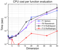
For the timing experiment the IPOP-^s∗aACM-ES was run on $f_{1}$ , $f_{8}$ , $f_{10}$ and $f_{15}$ without self-adaptation of surrogate model hyper-parameters. The crucial hyper-parameter for CPU time measurements, the number of training points was set $N_{training}=\left\lfloor 40+4D^{1.7}\right\rfloor$ as a function of dimension $D$ .

These experiments have been conducted on a single core with 2.4 GHz under Windows XP using Matlab R2006a.

On uni-modal functions the time complexity of surrogate model learning increases cubically in the search space dimension (see Fig. 1) and quadratically in the number of training points. For small dimensions ( $D<10$ ) the overall time complexity increases super-linearly in the dimension. The time complexity per function evaluation depends on the population size, because one model is used to estimate the ranking of all points of the population. This leads to a smaller computational complexity on multi-modal functions, e.g. $f_{15}$ Rastrigin function, where the population becomes much larger after several restarts.

The results presented here does not take into account the model hyper-parameters optimization, where $\lambda_{hyp}$ surrogate models should be build at each iteration, which leads to an increase of CPU time per function evaluation by a factor of $\lambda_{hyp}$ . For BIPOP-^s∗aACM-ES and IPOP-^s∗aACM-ES $\lambda_{hyp}$ was set to 20.

Refer to caption — Figure 1: CPU cost per function evaluation of IPOP-aACM-ES with fixed hyper-parameters.

5 Conclusion

In this paper, we have compared the recently proposed self-adaptive surrogate-assisted BIPOP-^s∗aACM-ES and IPOP-^s∗aACM-ES with the BIPOP-CMA-ES and IPOP-aCMA-ES. The surrogate-assisted ^s∗aACM-ES algorithms outperform the original ones by a factor from 2 to 4 on uni-modal functions, and usually perform not worse on multi-modal functions. The ^s∗aACM-ES algorithms improve the records on 8 out of 24 functions in dimension 10 and 20.

6 ACKNOWLEDGMENTS

The authors would like to acknowledge Anne Auger, Zyed Bouzarkouna, Nikolaus Hansen and Thomas P. Runarsson for their valuable discussions. This work was partially funded by FUI of System@tic Paris-Region ICT cluster through contract DGT 117 407 Complex Systems Design Lab (CSDL).

References

- [1] Z. Bouzarkouna, A. Auger, and D. Ding. Investigating the local-meta-model CMA-ES for large population sizes. In C. Di Chio et al., editor, Proc. EvoNUM’10, pages 402–411. LNCS 6024, Springer, 2010.
- [2] S. Finck, N. Hansen, R. Ros, and A. Auger. Real-parameter black-box optimization benchmarking 2009: Presentation of the noiseless functions. Technical Report 2009/20, Research Center PPE, 2009. Updated February 2010.
- [3] L. Graning, Y. Jin, and B. Sendhoff. Efficient evolutionary optimization using individual-based evolution control and neural networks: A comparative study. In Proc. ESANN’2005, pages 27–29, 2005.
- [4] N. Hansen. Benchmarking a BI-population CMA-ES on the BBOB-2009 function testbed. In Proceedings of the 11th Annual Conference Companion on Genetic and Evolutionary Computation Conference: Late Breaking Papers, GECCO ’09, pages 2389–2396, New York, NY, USA, 2009. ACM.
- [5] N. Hansen, A. Auger, S. Finck, and R. Ros. Real-parameter black-box optimization benchmarking 2012: Experimental setup. Technical report, INRIA, 2012.
- [6] N. Hansen, S. Finck, R. Ros, and A. Auger. Real-parameter black-box optimization benchmarking 2009: Noiseless functions definitions. Technical Report RR-6829, INRIA, 2009. Updated February 2010.
- [7] N. Hansen and A. Ostermeier. Completely derandomized self-adaptation in evolution strategies. Evolutionary Computation, 9(2):159–195, 2001.
- [8] N. Hansen and R. Ros. Benchmarking a weighted negative covariance matrix update on the BBOB-2010 noiseless testbed. In GECCO ’10: Proceedings of the 12th annual conference comp on Genetic and evolutionary computation, pages 1673–1680, New York, NY, USA, 2010. ACM.
- [9] F. Hoffmann and S. Holemann. Controlled model assisted evolution strategy with adaptive preselection. In International Symposium on Evolving Fuzzy Systems, pages 182–187. IEEE, 2006.
- [10] H. Ingimundardottir and T. Runarsson. Sampling strategies in ordinal regression for surrogate assisted evolutionary optimization. In Proc. ISDA’2011, page To appear, 2011.
- [11] G. A. Jastrebski and D. V. Arnold. Improving evolution strategies through active covariance matrix adaptation. In Proc. CEC’2006, pages 2814–2821, 2006.
- [12] S. Kern, N. Hansen, and P. Koumoutsakos. Local meta-models for optimization using evolution strategies. In Th. Runarsson et al., editor, PPSN IX, pages 939–948. LNCS 4193, Springer, 2006.
- [13] O. Kramer. Covariance matrix self-adaptation and kernel regression - perspectives of evolutionary optimization in kernel machines. Fundam. Inf., 98:87–106, 2010.
- [14] I. Loshchilov, M. Schoenauer, and M. Sebag. Comparison-Based Optimizers Need Comparison-Based Surrogates. In J. K. R. Schaefer, C. Cotta and G. Rudolph, editors, Proc. PPSN XI, pages 364–373. LNCS 6238, Springer, 2010.
- [15] I. Loshchilov, M. Schoenauer, and M. Sebag. Self-Adaptive Surrogate-Assisted Covariance Matrix Adaptation Evolution Strategy. In GECCO ’12: Proceedings of the 14th annual conference on Genetic and evolutionary computation, page to appear, New York, NY, USA, 2012. ACM.
- [16] K. Price. Differential evolution vs. the functions of the second ICEO. In Proceedings of the IEEE International Congress on Evolutionary Computation, pages 153–157, 1997.
- [17] T. P. Runarsson. Ordinal regression in evolutionary computation. In Th. Runarsson et al., editor, PPSN IX, pages 1048–1057. LNCS 4193, Springer, 2006.
- [18] H. Ulmer, F. Streichert, and A. Zell. Evolution strategies assisted by gaussian processes with improved pre-selection criterion. In Proc. CEC’2003, pages 692–699, 2003.