GLAS-PPE/2012-01
We consider and models recently proposed to explain the top forward-backward asymmetry at the Tevatron. We present the next-to-leading order QCD corrections to associated production of such vector bosons together with top quarks at the Large Hadron Collider, for centre-of-mass energies of 7 and 8 TeV. The corrections are significant, modifying the total production cross-section by 30-50%. We consider the effects of the corrections on the top and vector-boson kinematics. The results are directly applicable to current experimental searches, for both the ATLAS and CMS collaborations.
1 Introduction
Top-quark physics remains a highly active research area, both theoretically
and experimentally. The close proximity of the top-quark mass to the
electroweak symmetry breaking scale, and the possible role of new physics in
explaining this symmetry breaking, mean that the top-quark sector may provide
a clear window through which to look for beyond the Standard Model effects.
Furthermore, the Large Hadron Collider offers top-quark production rates far
in excess of previous colliders, allowing detailed scrutiny of the top quark
and its interactions. A complementary view is provided by the Tevatron which,
despite having a lower centre of mass energy, has an antisymmetric ()
initial state, which can probe different aspects of top-quark behaviour to the
LHC. One such feature is the forward-backward asymmetry of
pairs, which has been measured to be in excess of the Standard Model prediction [1, 2, 3, 4, 5, 6, 7] by both D0 and CDF [8, 9, 10], and
which has generated much subsequent theoretical interest.
In this paper we focus on a particular new physics scenario motivated by the
forward-backward asymmetry, namely the existence of and
(flavour-changing) bosons. These have been considered in a number
of recent studies (see e.g. [11, 12, 13, 14, 15, 16, 17, 18, 19, 20, 21, 22, 23, 24, 25, 26, 27, 28, 29, 30, 31, 32, 33, 34, 35, 36, 37, 38]). In some of these works (e.g. [14]), the new
gauge bosons emerge from a complete beyond the Standard Model theory with
extended gauge group. In other more phenomenological studies, the fundamental
origin of the new gauge bosons is not spelled out explicitly. This is
sufficient for the study of particular scattering processes, in that the
interaction Lagrangian for a or boson with Standard Model quarks
can be written in a generic form which is independent of the underlying
theory. Note also that coupling and parameter definitions (including overall
normalisations) differ in the above literature. Here we will focus our
discussion explicitly on the model of [29].
Although motivated by the sizeable forward-backward asymmetry, and
models must face a number of stringent experimental constraints, including
precision electroweak observables [39]; the neutron electric
dipole moment [40, 41]; same-sign top
production [42, 43]; the top-quark pair production cross-section
at the Tevatron [44, 45] and
LHC [46, 47]; and the top-quark charge asymmetry at the
LHC [48, 49]. As recent analyses have pointed
out [32, 31, 50], there is already tension between existing
constraints and theoretical predictions, such that significant fractions of
parameter space in such models are already being ruled out. In particular,
there seems to be some incompatibility between the measured LHC charge
asymmetry, and the Tevatron forward-backward asymmetry, if both are to have
a common origin in terms of - and -boson exchange.
Given the above experimental constraints on and models, it is also
important, experimentally, to explore every possible production
mechanism involving and bosons, so that cross-checks can be made of
the conclusions reached from different observables. A crucial process in this
regard is the direct production of such a gauge boson in association with a
single top quark, and indeed this process is being actively sought by the
ATLAS, CDF [51] and CMS [52]
collaborations 111Analyses may differ in whether they choose to focus
explicitly on the kinematic region of resonant gauge boson production, as we
discuss further in section 5.. These
searches result in direct bounds on the masses of the new gauge bosons, and
on their couplings to the quarks. These are upper and lower bounds for the
couplings and masses respectively, and in order for these to be as tight as
possible, it is preferable to include higher order perturbative corrections to
the relevant cross-sections.
The aim of this paper is to present the complete NLO QCD corrections to the
production of a or boson in association with a top (or anti-top) quark,
for both total cross sections and kinematic distributions of the top quark
and new gauge bosons. Our results can be used directly in relevant experimental
analyses, where they can be used to strengthen the bounds on the parameter
space of models involving these bosons. Our intention is to be as
model-independent as possible, so that our results can be combined to yield
total cross sections for various scenarios. We will see that NLO corrections
are significant for total rates (potentially of the order of 50% for central
values, and rising with the mass of the gauge boson), which by itself
justifies the calculation of higher-order corrections, due to the potentially
significant impact on extracted bounds on parameter space.
The structure of the paper is as follows. In section 2, we describe technical details relating to our NLO calculation, noting similarities to Standard Model production, which was first considered in [53], and calculated at NLO in [54, 55]. In section 3 we present results for total cross sections, examining also kinematic distributions in section 4. In section 5 we consider the implications of our results for current LHC searches. In section 6, we discuss our results before concluding. Various additional results are collected in the supplementary material accompanying this submission, which can be found in Appendix A of this preprint version.
2 Calculation of NLO corrections
In this section, we describe the technical details of our NLO calculation. Note
that many of these details are very similar to the (Standard Model)
calculation presented in [56], thus we will be brief.
Unless otherwise stated, we will explicitly refer to top-quark production as
opposed to antitop-quark production. Similar remarks apply in the latter case.
We consider NLO QCD corrections to the process
| (1) |
where is an appropriate quark, and is either a or boson. The LO diagrams are shown in figure 1.

Following [29], we define the coupling of these bosons to the top quark according to the Lagrangians
| (2) |
where is a coupling constant, the right-handed projection
operator, and , denote generic up-type and down-type quarks. The model
of [29] considers only couplings between the first and third
quark generations. In order to increase the flexibility of our calculation, we
here generalise this by including also couplings between the top quark and arbitrary
up and down-type quarks. The additional coupling factors and
play a role analogous to CKM matrix elements. Note that we carry out our
calculation in a five-flavour parton scheme, so that initial states involving
quarks are also included in the total cross section.
Note that the Lagrangian of eq. (4) is specific in the sense
that the coupling involves the pure right-handed projection operator .
In principle, there could be a mixture of left- and right-handed projectors,
with corresponding couplings and . However, analogously to
Standard Model production up to NLO [54, 55], the total cross section is
proportional to the combination . Hence, total cross sections
and kinematic distributions of the top and gauge bosons can be simply rescaled
in the presence of both left- and right-handed couplings. Note, however, that
the relative mixture of these would be important in considering distributions
relating to the decay products of the top quark and gauge boson.
As in [56, 57], we use the on-shell scheme for
renormalisation of the top-quark mass and QCD coupling [58]
(this modifies the -scheme renormalisation of the latter, such
that the top-quark loop contribution is subtracted on-shell).
The Feynman diagrams for the virtual corrections are exactly the same as those
for Standard Model production [54, 55], although
all finite parts of scalar integrals must be analytically continued to the
kinematic region . We use the results of [59], as
implemented in a previous calculation involving one of the
authors [57].
For the real emission corrections, all Feynman diagrams have the same form
as Standard Model production, for which we use results from a previous
calculation involving one of the present authors [56].
In the latter case, however, an on-shell subtraction scheme is necessary in
order to define the scattering process at NLO i.e. by removing the
contribution from leading order top pair
production [60, 61, 62, 56, 63, 64]. Here no such difficulties arise, due to the fact that
we explicitly consider the regime . Further differences with
production arise in that the partonic channels are different in the present
case. One must also replace the electroweak coupling and CKM matrix with the
relevant coupling factors from eq. (4).
In order to be able to numerically compute cross sections in a stable manner, the real and virtual corrections must be regularised and combined using an appropriate subtraction formalism for soft and collinear singularities, of which a number exist in the literature [65, 66, 67, 68, 69]. Here, as in [56], we use the FKS formalism of [65].
3 Total cross section for and production
In this section, we present results for total NLO cross sections, for the
process of eq. (1). For ease of comparison with
e.g. [29], we begin by considering the Lagrangian of
eq. (4) with a non-zero coupling between the first and third
generations only. That is, and .
Furthermore, we fix , and use default renormalisation and
factorisation scale choices of , where is the
mass of the or boson, as appropriate, and GeV is the top
quark mass. We consider the LHC, with a centre of mass energy of 7 TeV.
Results for the total cross section (i.e. the sum of both top and antitop
production) at LO and NLO are shown for both and production in
tables 1–4. We show all results using both
CTEQ [70, 71]222For ease of comparison with
existing literature, we provide results with CTEQ6L1 partons at LO.
and MSTW [72] partons,
where appropriate we calculate the parton distribution function (PDF) uncertainty using the relevant PDF
error sets. In all subsequent plots, we show results using MSTW partons unless
otherwise stated. For each result, we also present the scale variation
uncertainty obtained by varying both and independently in the
range , where is the default scale. One sees that the
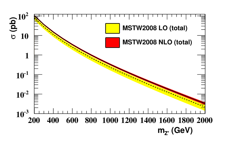
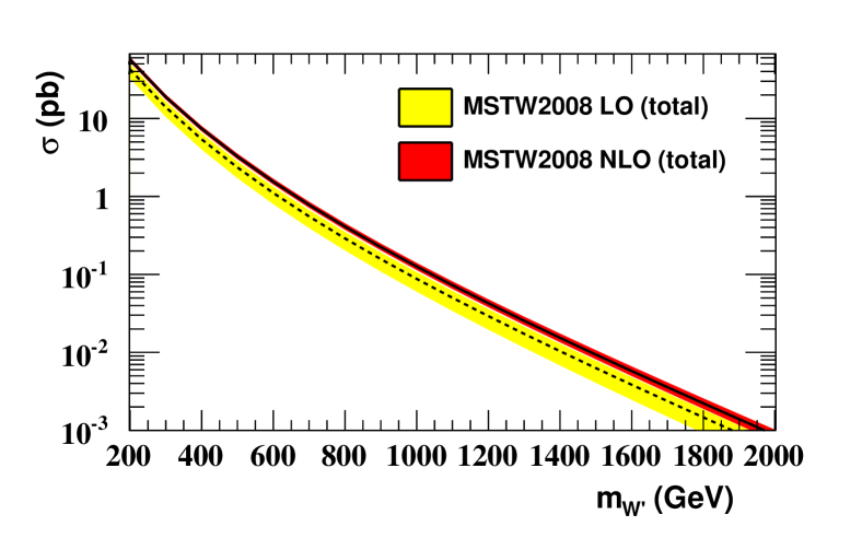
scale variation uncertainty is reduced at NLO, as expected. Furthermore, the
PDF uncertainty with MSTW partons is much smaller than the scale uncertainty.
This is also to be
expected, given that the cross section is dominated by the production of top
quarks involving a or quark in the initial state (for and
production respectively), namely valence quarks. Furthermore, the heavy nature
of the final state (involving both a top quark and a heavy vector boson) means
that the partons are evaluated at typically high momentum fractions .
Valence quark distributions at high are well constrained by global PDF
fits, hence the small PDF uncertainty in the results of
tables 1-4. With CTEQ partons the PDF uncertainty is of a similar size to the scale uncertainty over most of the mass range, becoming larger than the scale uncertainty at very high mass. This larger PDF uncertainty is partly due to the fact that the CTEQ uncertainties represent 90% confidence intervals whereas the MSTW uncertainties represent 68% confidence intervals333This is typically accounted for by dividing the CTEQ uncertainties by a factor 1.645 [73].. Plots of the total cross sections for
and production are shown in figures 2 and 3,
where we have added the PDF and scale uncertainties in quadrature.
| (GeV) | (pb) | (pb) | |||||
|---|---|---|---|---|---|---|---|
| 200 | 77. | 9 | 79. | 3 | |||
| 300 | 26. | 65 | 27. | 28 | |||
| 400 | 10. | 81 | 11. | 15 | |||
| 500 | 4. | 89 | 5. | 08 | |||
| 600 | 2. | 39 | 2. | 50 | |||
| 700 | 1. | 234 | 1. | 306 | |||
| 800 | 0. | 667 | 0. | 713 | |||
| 900 | 0. | 373 | 0. | 402 | |||
| 1000 | 0. | 215 | 0. | 234 | |||
| 1100 | 0. | 126 | 0. | 139 | |||
| 1200 | 0. | 0759 | 0. | 0840 | |||
| 1300 | 0. | 0463 | 0. | 0516 | |||
| 1400 | 0. | 0286 | 0. | 0321 | |||
| 1500 | 0. | 0178 | 0. | 0202 | |||
| 1600 | 0. | 0112 | 0. | 0128 | |||
| 1700 | 0. | 0071 | 0. | 0082 | |||
| 1800 | 0. | 00455 | 0. | 00527 | |||
| 1900 | 0. | 00292 | 0. | 00340 | |||
| 2000 | 0. | 00188 | 0. | 00220 | |||
| (GeV) | (pb) | (pb) | |||||
|---|---|---|---|---|---|---|---|
| 200 | 41. | 8 | 42. | 7 | |||
| 300 | 13. | 60 | 13. | 92 | |||
| 400 | 5. | 26 | 5. | 41 | |||
| 500 | 2. | 28 | 2. | 35 | |||
| 600 | 1. | 068 | 1. | 109 | |||
| 700 | 0. | 531 | 0. | 554 | |||
| 800 | 0. | 276 | 0. | 290 | |||
| 900 | 0. | 149 | 0. | 157 | |||
| 1000 | 0. | 0829 | 0. | 0879 | |||
| 1100 | 0. | 0472 | 0. | 0502 | |||
| 1200 | 0. | 0274 | 0. | 0293 | |||
| 1300 | 0. | 0161 | 0. | 0173 | |||
| 1400 | 0. | 0097 | 0. | 0104 | |||
| 1500 | 0. | 0058 | 0. | 0063 | |||
| 1600 | 0. | 00356 | 0. | 00386 | |||
| 1700 | 0. | 00218 | 0. | 00238 | |||
| 1800 | 0. | 00135 | 0. | 00147 | |||
| 1900 | 0. | 00084 | 0. | 00092 | |||
| 2000 | 0. | 00052 | 0. | 00057 | |||
| (GeV) | (pb) | (pb) | ||||||
|---|---|---|---|---|---|---|---|---|
| 200 | 101. | 2 | 103. | 6 | ||||
| 300 | 35. | 32 | 36. | 10 | ||||
| 400 | 14. | 61 | 14. | 92 | ||||
| 500 | 6. | 74 | 6. | 87 | ||||
| 600 | 3. | 35 | 3. | 41 | ||||
| 700 | 1. | 769 | 1. | 795 | ||||
| 800 | 0. | 975 | 0. | 987 | ||||
| 900 | 0. | 557 | 0. | 561 | ||||
| 1000 | 0. | 327 | 0. | 328 | ||||
| 1100 | 0. | 197 | 0. | 196 | ||||
| 1200 | 0. | 121 | 0. | 120 | ||||
| 1300 | 0. | 0752 | 0. | 0740 | ||||
| 1400 | 0. | 0475 | 0. | 0463 | ||||
| 1500 | 0. | 0303 | 0. | 0293 | ||||
| 1600 | 0. | 0195 | 0. | 0187 | ||||
| 1700 | 0. | 0127 | 0. | 0120 | ||||
| 1800 | 0. | 0083 | 0. | 0078 | ||||
| 1900 | 0. | 0055 | 0. | 0050 | ||||
| 2000 | 0. | 00360 | 0. | 00328 | ||||
| (GeV) | (pb) | (pb) | ||||||
|---|---|---|---|---|---|---|---|---|
| 200 | 55. | 6 | 57. | 1 | ||||
| 300 | 18. | 48 | 18. | 83 | ||||
| 400 | 7. | 32 | 7. | 40 | ||||
| 500 | 3. | 24 | 3. | 25 | ||||
| 600 | 1. | 555 | 1. | 546 | ||||
| 700 | 0. | 792 | 0. | 780 | ||||
| 800 | 0. | 423 | 0. | 411 | ||||
| 900 | 0. | 234 | 0. | 225 | ||||
| 1000 | 0. | 134 | 0. | 127 | ||||
| 1100 | 0. | 0781 | 0. | 0729 | ||||
| 1200 | 0. | 0466 | 0. | 0428 | ||||
| 1300 | 0. | 0283 | 0. | 0255 | ||||
| 1400 | 0. | 0174 | 0. | 0154 | ||||
| 1500 | 0. | 0108 | 0. | 0094 | ||||
| 1600 | 0. | 0068 | 0. | 0058 | ||||
| 1700 | 0. | 00434 | 0. | 00358 | ||||
| 1800 | 0. | 00277 | 0. | 00223 | ||||
| 1900 | 0. | 00178 | 0. | 00139 | ||||
| 2000 | 0. | 00115 | 0. | 00087 | ||||
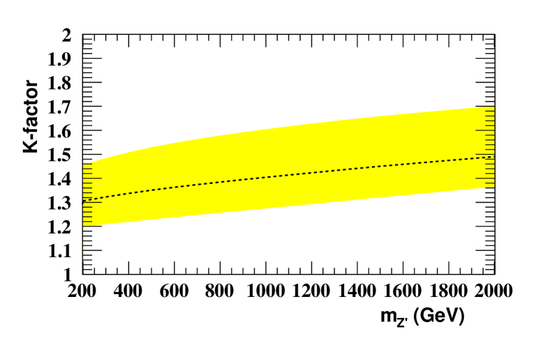
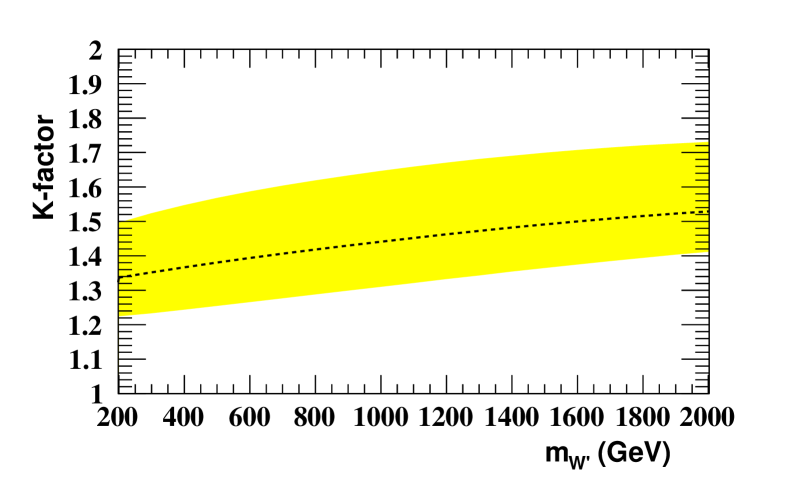
In figures 4 and 5, we show the -factor for both and production as a function of the mass of the gauge boson , evaluated according to
| (3) |
where we have used the results obtained with MSTW partons from
tables 1-4. We see that the -factor is sizeable
and increasing with . For the values of we consider, the NLO
corrections range from in both cases. This can be compared
with Standard Model production, for which the -factor is
[54, 55], subject to an appropriate
on-shell subtraction formalism being employed to separate the mode from
top pair production. The higher factor in the present case, and the fact
that the -factor rises with increasing gauge boson mass, have partonic
origins. As stated above, both and production have valence quarks
in the initial state. Furthermore, as increases, these distributions
are probed at typically higher values, and relatively more so at NLO.
Given that valence quark distributions remain significant at higher values,
the -factor is therefore sizable. One may find the opposite trend if sea or
quarks are involved in the initial state i.e. a
-factor which decreases with increasing , due to the sharp fall-off in
the partons as (we consider other partonic couplings in
the supplementary document). Note that there are
also extra partonic subchannels which open up at NLO (i.e. the and
initial states), which also act to increase the -factor.
From tables 1–4 and
figures 4–5, one sees that the -factor for
production is slightly larger than that for production.
This can be explained by the fact that the former case has quarks in the
initial state rather than quarks. The heavy final state means that these
partons are typically probed at high values, where the quark
distribution (at LO or NLO) has a pronounced shoulder (followed by a steep fall off)
relative to the quark distribution [72]. At NLO, the
partons are probed at higher values than at LO, which leads to a decrease
in the parton luminosity. This is less marked for the distribution than for
the distribution, due to the shoulder in the latter. Hence, the -factor
for production is slightly larger than that for
production 444Another reason for the -factor difference is due to
additional partonic subchannels opening up at NLO, with and
initial states, which contribute different fractions of the total
cross-sections in and production. However, this has a small effect
on the -factor difference, due to the fact that the NLO cross-section
remains dominated by initial states..
As well as the total cross section, it is also interesting to consider the
fraction of events containing a top quark, rather than an anti-top quark (in
the case of production, this changes the sign of the charge of the
accompanying boson).
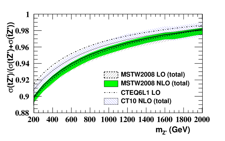
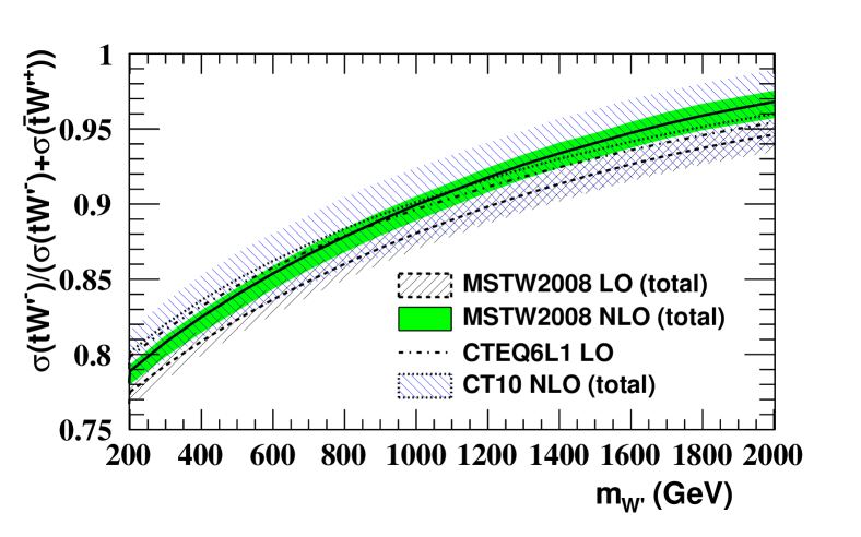
This fraction is shown for and production in
figures 6 and 7 respectively, at both LO and NLO.
We see in both cases that the total cross section is dominated by quark
production, due to the presence of valence rather than sea quarks in the
initial state at LO. Furthermore, we note that the theoretical uncertainty is dominated by PDF uncertainties rather than scale variation, as the latter effect is similar for top and anti-top production, and cancels in the ratio.
The top quark fraction is higher for rather than
production, due to the dominance of up quarks over down quarks in the proton.
Note that the fractions increase with the gauge boson mass, reflecting the
fact that the partons are evaluated at higher values on average as the
gauge boson mass increases, which causes sea-quark dominated processes to
fall off at the expense of those which are dominated by valence quarks.
We may also note that the fraction changes slightly at NLO, and can either
decrease or increase, depending on the gauge boson mass. This is due to two
competing effects. Firstly, extra partonic subchannels open up at NLO which are
insensitive to the exchange of a top and anti-top quark. This acts to decrease
the fraction of top quark events. Secondly, the partons are evaluated at
slightly higher values at NLO compared to LO. This increases the dominance
of valence quark-initiated processes, and acts to increase the proportion of
top quark events. The size of the latter effect is somewhat uncertain due to
the influence of high- sea quark distributions. This can clearly be seen
in both figures 6 and 7, where we show the
top quark fraction for CTEQ as well as MSTW partons. The CTEQ results lead to
higher top-quark fractions, with a decrease at NLO (apart from production
at low gauge boson masses). In the MSTW results, there is an increase in the
top-quark fraction at NLO, suggesting that valence quark distribution
effects are more dominant.
In this section, we have considered a subset of possible couplings in eq. (4), in particular considering only the and interactions for and respectively. In the supplementary material, we present tables of results for other possible choices. Furthermore, we present results for the LHC at 8 TeV. Having discussed the total cross-section results in detail, we discuss NLO corrections to kinematic distributions of the top quark and gauge bosons in the following section.
4 Top and heavy gauge boson kinematics
In this section, we examine the impact of NLO QCD corrections on various
kinematic distributions relating to the top quark and gauge boson. Throughout,
we use the parameter choices described in the previous section, with MSTW LO
and NLO partons [72] as appropriate.
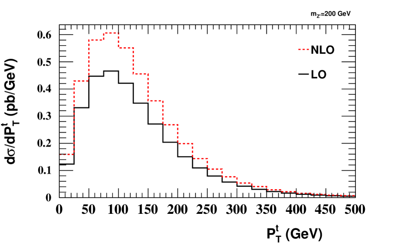
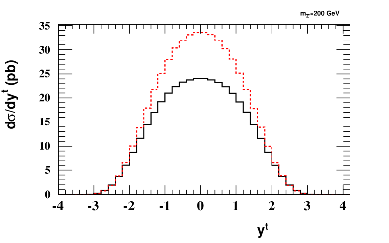
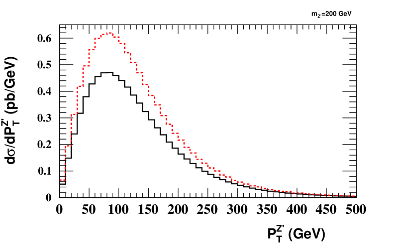
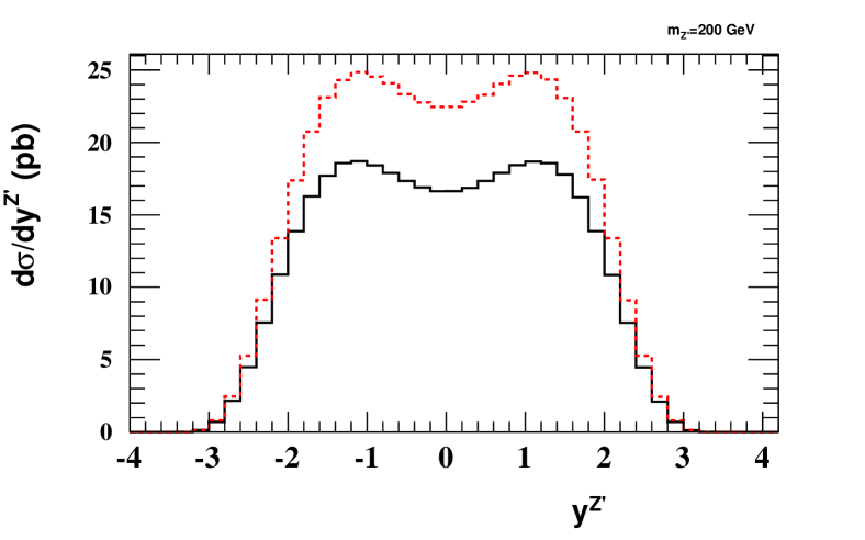
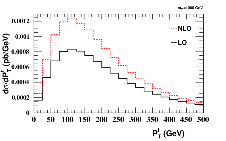
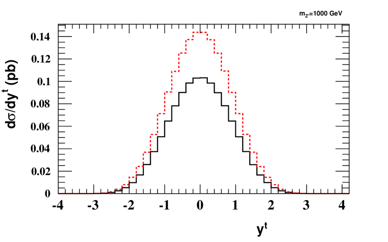
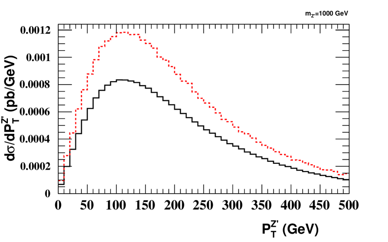
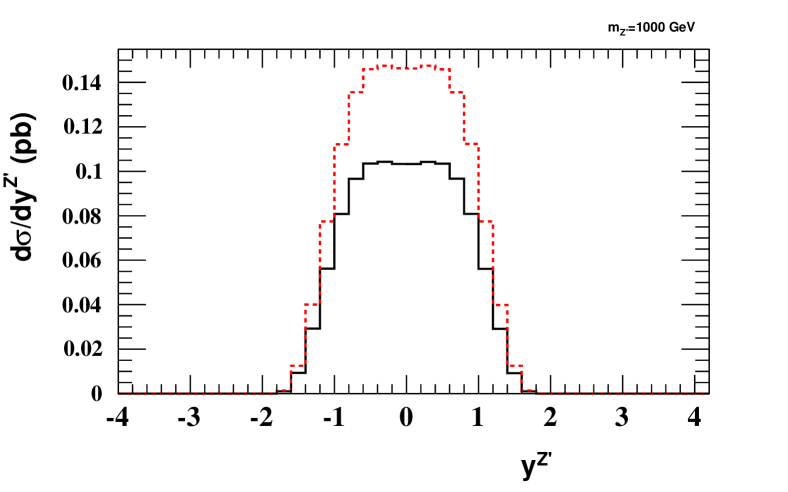
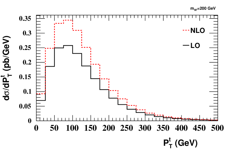
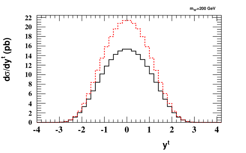
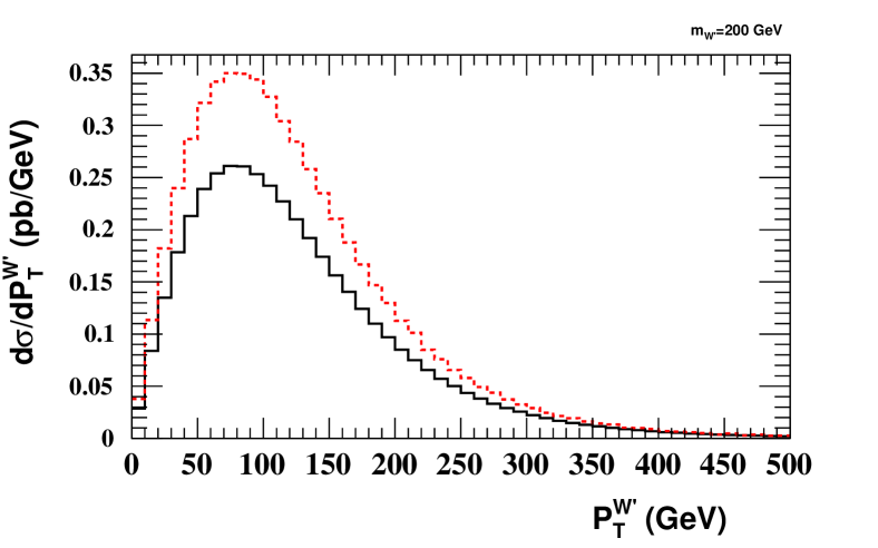
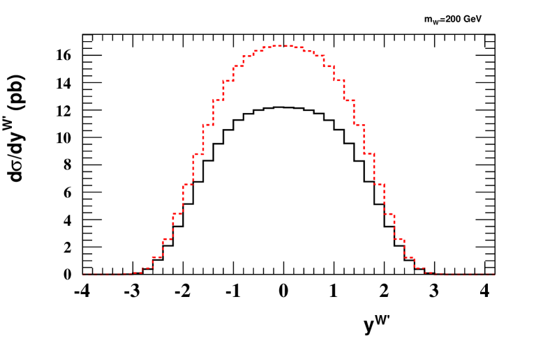
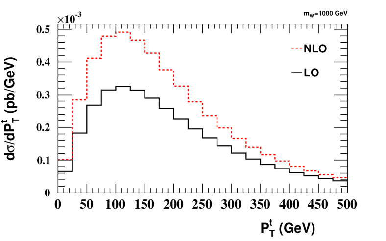
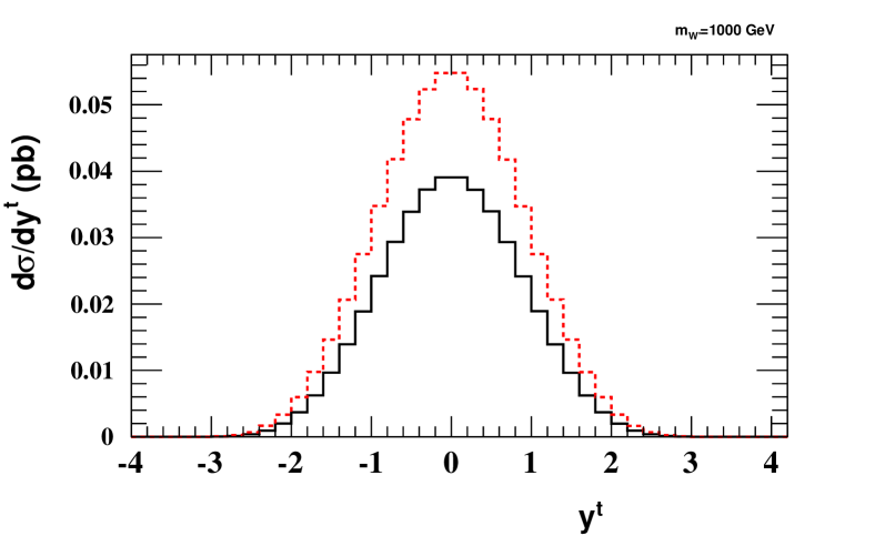
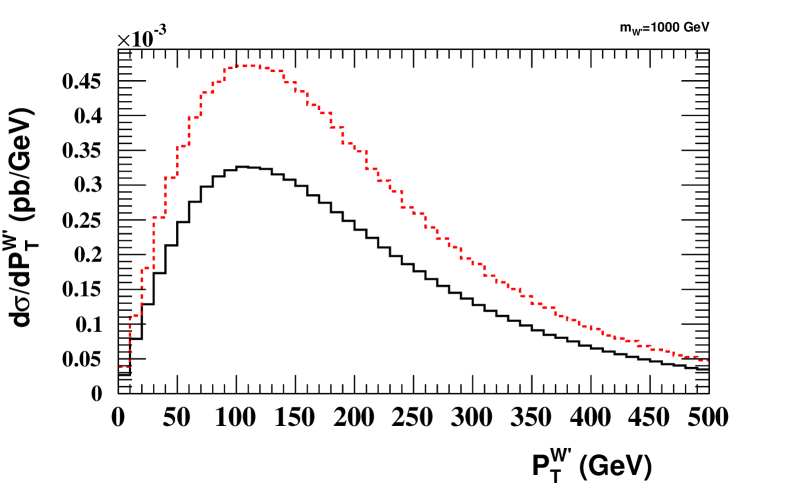
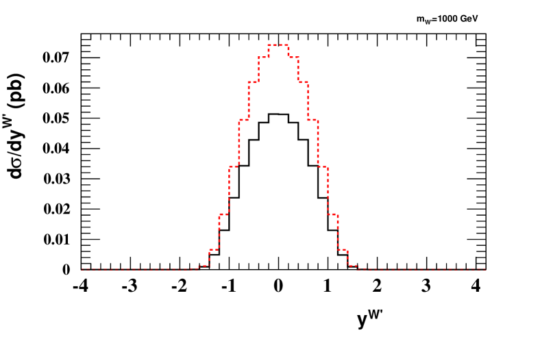
In figure 8, we show the
transverse-momentum and rapidity distributions for the top quark and gauge
boson in production, for masses of 200 GeV and 1000 GeV respectively. One
sees that the top quark has a wide rapidity distribution peaking at zero, whereas
the boson is preferentially produced in either the forward or backward
direction. This is due to the fact that we are here considering the
case of production via coupling of the top to an up quark. The latter is a
valence quark, and thus carries more momentum on average than the initial
state gluon. This results in a boosted final state, where the boson is
preferentially emitted in the direction of the incoming up quark, from
helicity considerations. The double peak structure will be absent for couplings
between the top and second generation quarks, or for antitop production, as
there is then no valence quark in the initial state.
Furthermore, the rapidity distributions become narrower as the gauge boson mass
increases, reflecting the fact that production becomes more central for heavier
final states. This is also reflected in the fact that the peaks of the
transverse momentum distributions (for both the top quark and gauge boson)
shift upwards as the gauge boson mass increases.
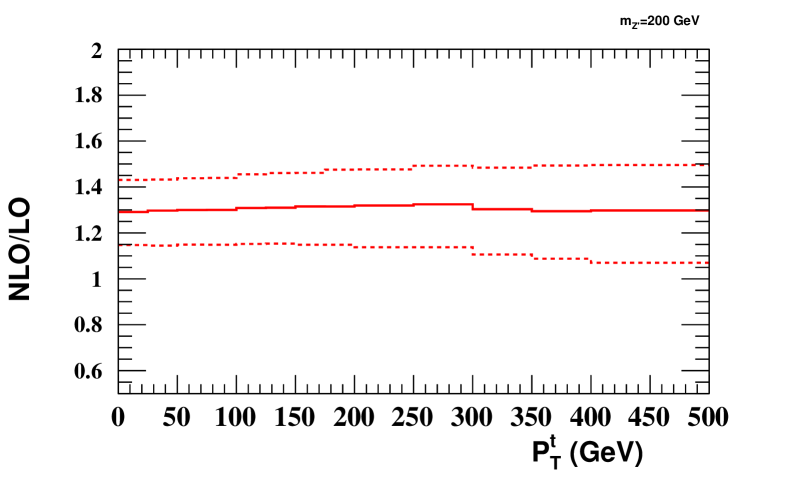
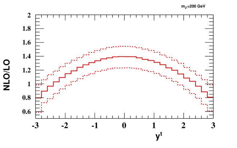
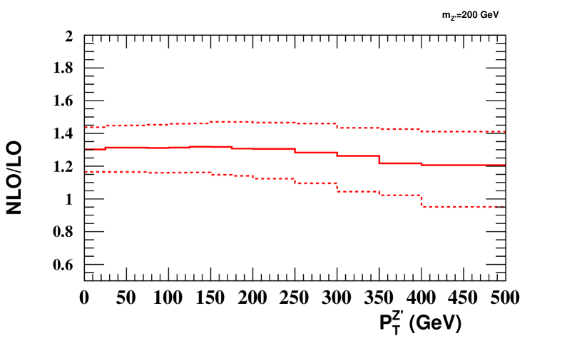
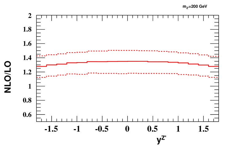
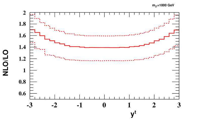
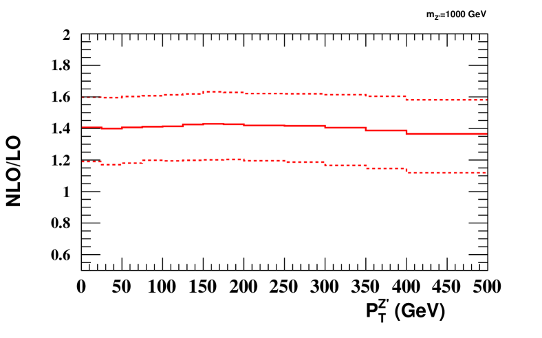
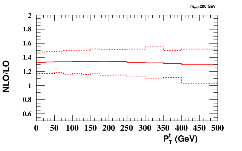
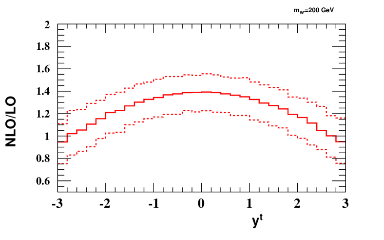
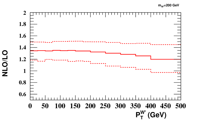
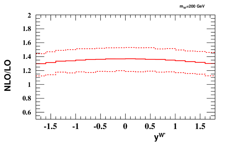
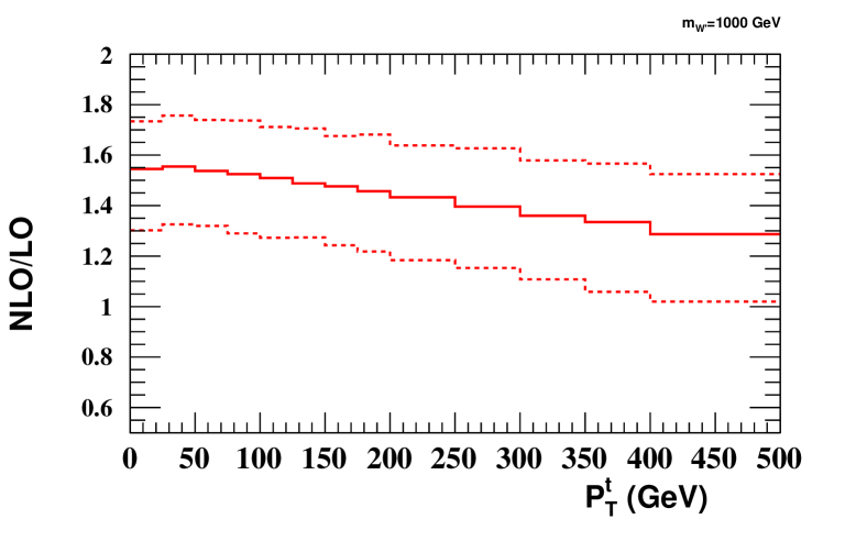
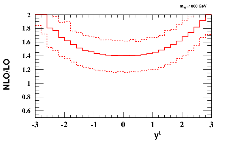
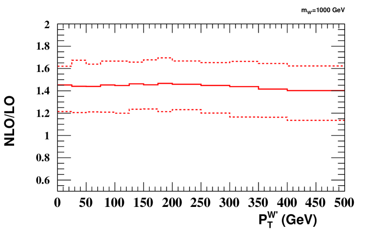
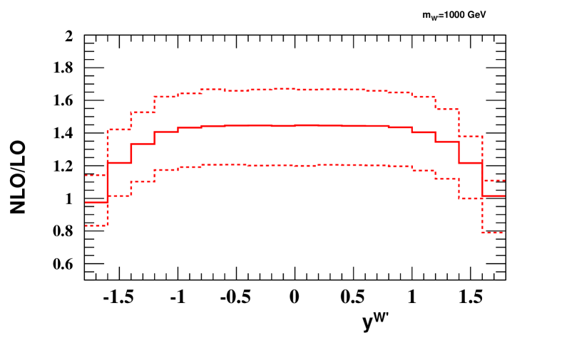
We show the ratio of the NLO and LO results for the above distributions
for a 200 GeV gauge boson in figure 9. One sees
that for lower gauge boson masses, NLO corrections have little impact on the
shape of the transverse momentum distributions of the top quark or boson
(although the tails of the NLO distributions are slightly softer, as expected).
This can be understood by the fact that QCD radiation is dominated by
emissions which are collinear to the incoming particles: the
heavy final state limits the phase space for hard gluon emission, and contains
a non-radiating colour-singlet particle and a heavy quark, such that there are
no final state collinear singularities. This expectation is confirmed in
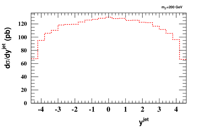
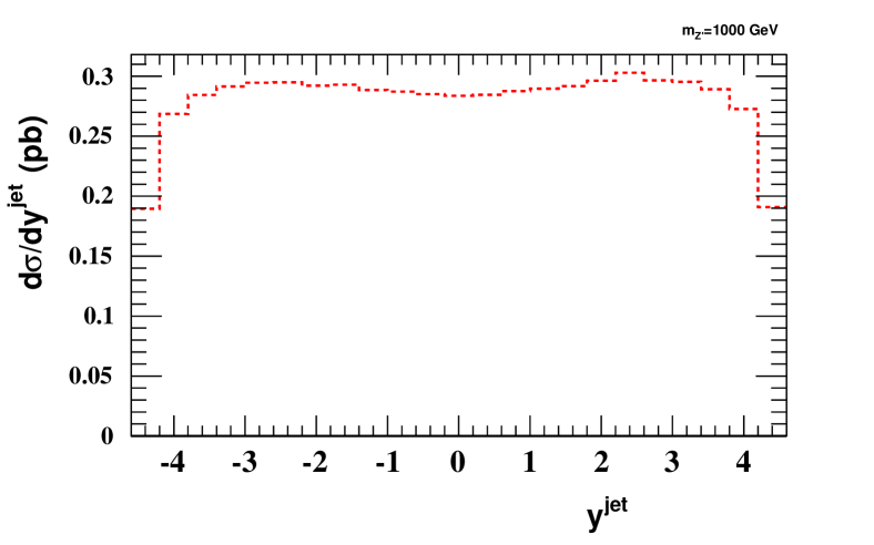
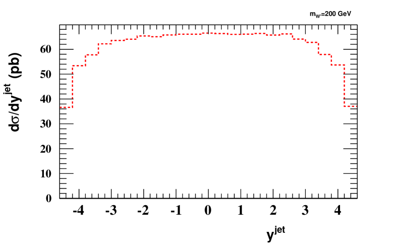
figure 10, which shows the rapidity distribution of the
additional parton emitted at NLO. The distribution is wide and flat, and thus
characteristic of initial state radiation. This acts to make the rapidity
distributions of the and more strongly peaked at central values (i.e.
there is less energy available to the pair), and thus to proportionally
reduce the double peak structure in the -boson rapidity distribution. Ratio
plots for a heavy gauge boson (1000 GeV) are also shown in
figure 9. Here one sees that the transverse momentum
of the top gets somewhat softer at NLO (more so than for lower gauge boson
masses), and also its rapidity distribution is slightly less central. This
can be understood by noting that the top quark is more energetic on average
for heavier gauge boson masses, due to momentum conservation. It can therefore
emit harder radiation, such that the jet and top quark are produced slightly
off-centre. This is borne out by the rapidity distribution of the extra parton
in figure 10, which shows a shape difference with respect
to the case of a 200 GeV boson.
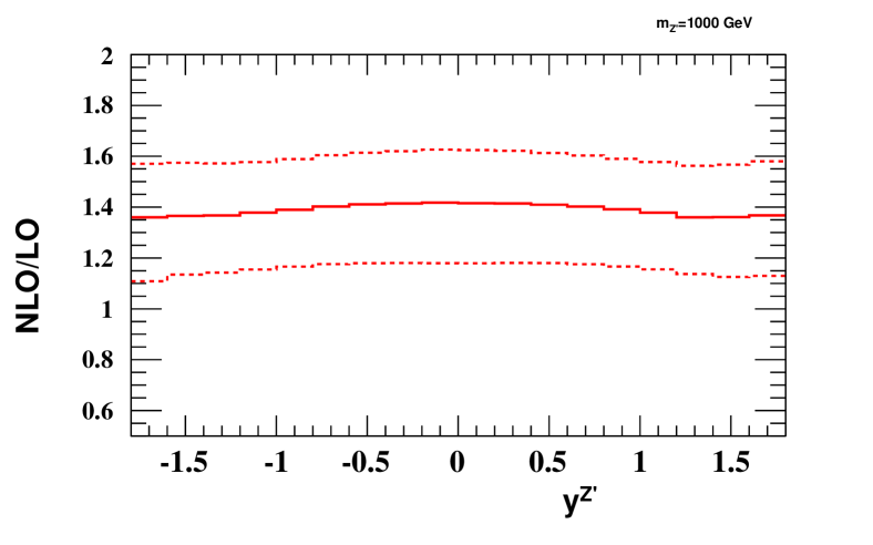
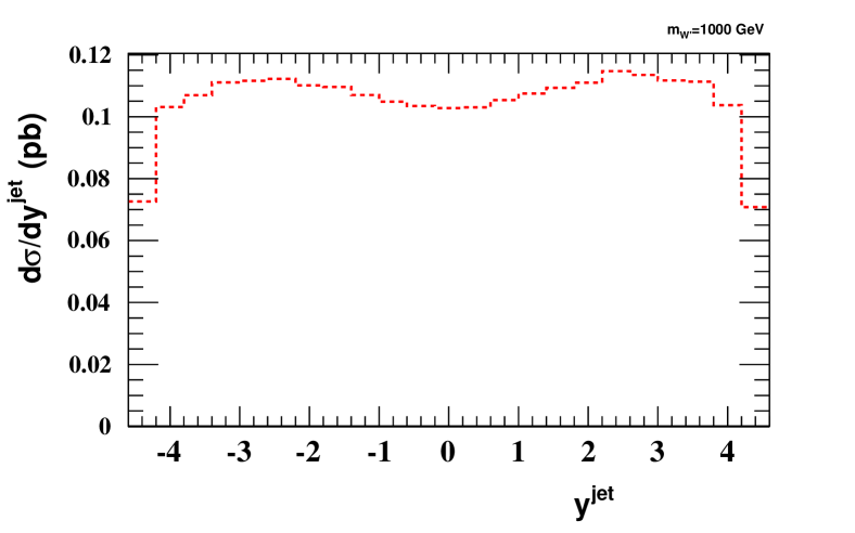
Analogous results for production are shown in
figure 11, again for gauge boson
masses of 200 GeV and 1000 GeV. Corresponding ratio plots are shown in
figure 12.
The results are broadly similar to the
results apart from one qualitiative feature: the lack of a double peak in the
-boson rapidity distribution. This is due to the fact that the initial state
contains a down rather than an up quark, which carries proportionally less
momentum, thus weakening the boost of the final state. A reasonable effect
persists however, as can be seen by the fact that the rapidity
distribution is noticeably wider than that of the top quark. Again, real
emission corrections are dominated by initial state radiation, which is born
out by the rapidity distribution of the extra parton in the lower panels
of figure 10. There is again a difference in how rapidity
distributions change at NLO in going from lower to higher gauge-boson masses,
due to the fact that final-state radiation from the top is harder on average
due to its recoiling against a highly massive boson.
In this and the previous section, we have examined the impact of NLO cross sections on total rates and distributions. A useful preliminary application of these results is to examine their impact on current searches for top-associated and production. This is the subject of the following section.
5 Implications for and searches
In this section we discuss the implications of our results for experimental
searches. As a specific example, we consider the impact on results from a recent ATLAS search [74, 75] for with , in order to illustrate the impact of the results in this paper.
Experimental searches for or production make use of LO Monte Carlo simulations, typically with events from the Madgraph [76] matrix element generator. We note that the latest release (2.6) of Herwig++ [77] also implements relevant models for and .
The cross-sections for the new-physics processes and kinematics of the top quark and associated heavy boson are generally derived from these LO codes. Correction of the cross section to the NLO values is straightforward using the results from Section 3 (see also the supplementary material for different coupling choices). Thus experimental upper limits on cross-sections correspond to stronger limits on the allowed couplings. Furthermore the reduced scale dependence at NLO means that a limit on the coupling that fully accounts for the uncertainty on the cross section would be substantially improved.
The kinematics of the top and associated heavy boson can also be corrected to account for the differing distributions at NLO. We stress that, since at NLO the top and heavy boson are produced more centrally, the acceptance would be higher for events produced at NLO than LO. It is thus the case that using LO samples to derive acceptance and set upper limits on cross sections is a conservative approach.
The charge asymmetry in the production rate of the top quarks from heavy boson decays can also be exploited in a search. The SM jet background is charge symmetric, so choosing to look at the anti-top+jet rather than top +jet mass spectrum can reduce the background by a factor of two while preserving the majority of signal. This is the case in the recent ATLAS search [75] where windows in the top+jet mass vs anti-top+jet mass plane that give optimal sensitivity to signal are chosen. We showed in Section 3 that this asymmetry is quite stable in moving from LO to NLO and have provided the necessary information to account for this effect.
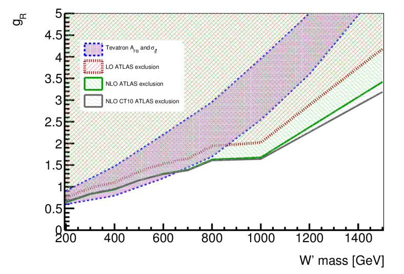
In order to demonstrate the impact of our NLO corrections, we first show in figure 13 a series of exclusion limits in the plane. The LO and NLO figures are obtained by taking the cross-section limit from the ATLAS search [74, 75], and using our LO and NLO calculations respectively, with scale choices and other parameters as defined in section 3. Also shown is the region favoured by the Tevatron forward-backward asymmetry measurements [8, 9], here taken from [75]. We see that NLO corrections significantly increase the constraints in parameter space, effectively cutting off most of the region that is still favoured by the Tevatron measurements. Whilst models do not have to explain the forward-backward asymmetry, this was a significant motivation for considering them in the first place. Thus, the fact that only a sliver of asymmetry-favoured space remains is an important result, justifying the calculation of NLO corrections.
A similar conclusion has been reached by the ATLAS collaboration itself, who have used the results of the present paper in their most up-to-date analysis [75]. Note that our NLO exclusion limits differ slightly from theirs, due to the fact that it has been calculated independently, using estimates of the cross-section limits presented in [74, 75]. Also, we have here used a default common factorisation and renormalisation scale of , as opposed to the fixed scale of 200 GeV used by ATLAS for their LO limit [74]. We do not see a motivation for the latter scale for high gauge boson masses. Nevertheless, the results are broadly similar to those of [75].
The CMS collaboration have also presented bounds on production [52]. However, unlike the ATLAS analysis, this bound is on the combination of the resonant process, and the -channel exchange process. One could take this to be a conservative estimate on the resonant process, but this would give a much weaker bound on the cross-section than would be obtained in practice. For this reason, we do not show the CMS result in figure 13, so as not to introduce an unfair comparison. Another reason for not including this is a recent study [78] showing that interference with SM jet production is important for the CMS search, and significantly weakens the limit. The effect of such interference is negligible for searches that focus on the resonant process.
Note that our analysis in this section is only an approximate estimate of the exclusion limits implied by our NLO calculation. Firstly, and as stated above, we have not taken into account explicitly that the theoretical uncertainty of the NLO cross-section (due predominantly to scale variation) is significantly reduced relative to LO. Secondly, we have not accounted for the change in kinematic distributions, which would affect the acceptance. There is also an important interplay between these direct searches and additional constraints such as those discussed in the introduction.
A more realistic analysis can be found in the ATLAS paper [75], but we think it still worth presenting an independent exclusion plot here. Firstly, it is interesting to note that a rough estimate gives results which are reasonably similar to the ATLAS analysis. Secondly, we use a more physically motivated scale choice, which can be much different to the fixed LO scale of 200 GeV used by [29] and the ATLAS analysis, at high gauge boson masses. It is reassuring to see that this does not lead to a large deviation from their results.
In this section, we have illustrated the impact of our NLO results in the well-studied case (both theoretically and experimentally) in which the top couples to the first generation quarks only. It is worth stressing that our NLO calculation would also be useful in scenarios with alternative coupling choices, where their impact may be larger.
6 Conclusion
In this paper, we have calculated NLO QCD corrections to the associated
production of and boson production with a top quark. This production
mode is being actively searched for by both the ATLAS and CMS collaborations,
and higher-order corrections are important in order to set tight bounds on
couplings and gauge boson masses, due to both the size of NLO effects, and the
requisite reduction in theoretical uncertainty. As we have seen, for models in
which the top quark couples to first generation quarks, the uncertainty is
dominated by scale variation, whereas the PDF uncertainty is small, due to
the fact that high- valence quark distributions are well-constrained in
global fits. One thus achieves a significant decrease in theoretical
uncertainty in going to NLO, as can be seen directly in the total cross-section
plots of figures 2 and 3.
Although we have focussed on the particular Lagrangian of
eq. (4), our analysis is more general in that one can
straightforwardly combine the results collected in the main body
of this paper and the supplementary material in order to generate total cross sections for models
which have non-trivial mixing between quark generations or a mixture of
left- and right-handed couplings. Thus, our results can be directly and
generally applied in current experimental analyses, which may differ somewhat
in the particular models which are being considered. Our aim has been to
provide as complete a set of numbers as possible for use in experimental
searches, including cross sections at a centre-of-mass energy of 8 TeV,
which can be found in the supplementary material. Results for alternative
parameter choices, if desired, may be requested by contacting the authors.
As well as total cross-sections, we also considered transverse momentum and
rapidity distributions of the top quark and gauge bosons. We find that NLO
corrections lead, predictably, to a softening of transverse momentum
distributions, which effect increases with the gauge boson mass. Rapidity
distributions are more affected even at low gauge boson masses, due to the fact
that real emission corrections are dominated by initial state radiation. The
top quark becomes more (less) central at low (high) gauge boson masses.
In section 5, we briefly examined the implications of our results
for current searches, and estimated how coupling and mass limits would change
in the recently presented ATLAS analysis of [75]. We find
that coupling bounds are strengthened by around 20%, and that the region favoured by the Tevatron forward-backward asymmetry is all but excluded. The latter is a significant result, given that this asymmetry is a major motivation for considering and models in the first place.
Our analysis is an approximate estimate, and could be enhanced by taking into account the fact that the theoretical uncertainty diminishes when NLO corrections are implemented, and that kinematic distributions change (affecting the acceptance of signal events).
To summarise, we have provided NLO QCD corrections for use in experimental searches for and bosons in association with a top quark. The hunt for such particles is ongoing.
Acknowledgements
This work was supported in part by grant DE-FG02-92ER40704 from the U.S. Dept. of Energy. We thank Daniel Whiteson for discussions and comments on the manuscript and Steven Worm for discussions regarding the CMS limits. JA thanks Moira I. Gresham, Ian-Woo Kim and Kathryn M. Zurek for useful discussions about the and models. JF is supported by the UK Science and Technology Facilities Council (STFC). CDW thanks Stefano Frixione for useful conversations, and also David Miller for discussions. He is supported by the STFC Postdoctoral Fellowship “Collider Physics at the LHC”.
Appendix A Supplementary material
In this supplementary material, we collect various additional results from our NLO and calculation, which are of further use for current (and future) experimental analyses. As in the main paper, we adopt the Lagrangians
| (4) |
where and are suitable mixing matrices. The main paper focuses on the cases (all other ). Here we consider other possible coupling choices, and also how to combine these in order to obtain total NLO cross-sections in general models. For completeness, we also give results for and production separately, beginning in the following section.
A.1 Cross-section results at 7 TeV separated by top charge
This section contains the total cross sections for and production separately. These are for cases where the () couples to (). For couplings to second and third generation quarks, no charge asymmetry is expected due to the equality for sea quark distributions555Modern PDF analyses typically allow [79, 80, 72]. However, this would result in a negligible charge asymmetry..
Tables 5 and 6 give the cross sections at LO for production where the is specifically a top quark and anti-top quark respectively. The NLO cross sections for the same process are given in Tables 7 and 8. The equivalent cross sections for production are given in Tables 9-12.
| (GeV) | (pb) | (pb) | |||||
|---|---|---|---|---|---|---|---|
| 200 | 6. | 51 | 8. | 04 | |||
| 300 | 1. | 89 | 2. | 41 | |||
| 400 | 0. | 66 | 0. | 87 | |||
| 500 | 0. | 262 | 0. | 353 | |||
| 600 | 0. | 113 | 0. | 156 | |||
| 700 | 0. | 052 | 0. | 073 | |||
| 800 | 0. | 0251 | 0. | 0363 | |||
| 900 | 0. | 0126 | 0. | 0187 | |||
| 1000 | 0. | 0066 | 0. | 0099 | |||
| 1100 | 0. | 0035 | 0. | 0054 | |||
| 1200 | 0. | 00193 | 0. | 00299 | |||
| 1300 | 0. | 00107 | 0. | 00169 | |||
| 1400 | 0. | 00061 | 0. | 00097 | |||
| 1500 | 0. | 00035 | 0. | 00056 | |||
| 1600 | 0. | 00020 | 0. | 00033 | |||
| 1700 | 0. | 000117 | 0. | 000195 | |||
| 1800 | 0. | 000069 | 0. | 000116 | |||
| 1900 | 0. | 000041 | 0. | 000069 | |||
| 2000 | 0. | 000024 | 0. | 000041 | |||
| (GeV) | (pb) | (pb) | |||||
|---|---|---|---|---|---|---|---|
| 200 | 71. | 3 | 71. | 2 | |||
| 300 | 24. | 74 | 24. | 85 | |||
| 400 | 10. | 14 | 10. | 27 | |||
| 500 | 4. | 62 | 4. | 73 | |||
| 600 | 2. | 27 | 2. | 35 | |||
| 700 | 1. | 181 | 1. | 232 | |||
| 800 | 0. | 641 | 0. | 676 | |||
| 900 | 0. | 360 | 0. | 383 | |||
| 1000 | 0. | 208 | 0. | 224 | |||
| 1100 | 0. | 123 | 0. | 133 | |||
| 1200 | 0. | 0739 | 0. | 0809 | |||
| 1300 | 0. | 0451 | 0. | 0499 | |||
| 1400 | 0. | 0279 | 0. | 0311 | |||
| 1500 | 0. | 0175 | 0. | 0196 | |||
| 1600 | 0. | 0110 | 0. | 0125 | |||
| 1700 | 0. | 0070 | 0. | 0080 | |||
| 1800 | 0. | 00448 | 0. | 00515 | |||
| 1900 | 0. | 00288 | 0. | 00333 | |||
| 2000 | 0. | 00186 | 0. | 00216 | |||
| (GeV) | (pb) | (pb) | ||||||
|---|---|---|---|---|---|---|---|---|
| 200 | 9. | 17 | 10. | 31 | ||||
| 300 | 2. | 74 | 3. | 09 | ||||
| 400 | 0. | 99 | 1. | 12 | ||||
| 500 | 0. | 402 | 0. | 457 | ||||
| 600 | 0. | 178 | 0. | 203 | ||||
| 700 | 0. | 085 | 0. | 096 | ||||
| 800 | 0. | 0422 | 0. | 0479 | ||||
| 900 | 0. | 0219 | 0. | 0248 | ||||
| 1000 | 0. | 0118 | 0. | 0132 | ||||
| 1100 | 0. | 0065 | 0. | 0073 | ||||
| 1200 | 0. | 0037 | 0. | 0041 | ||||
| 1300 | 0. | 00210 | 0. | 00231 | ||||
| 1400 | 0. | 00123 | 0. | 00134 | ||||
| 1500 | 0. | 00073 | 0. | 00078 | ||||
| 1600 | 0. | 00043 | 0. | 00046 | ||||
| 1700 | 0. | 000262 | 0. | 000272 | ||||
| 1800 | 0. | 000159 | 0. | 000162 | ||||
| 1900 | 0. | 000097 | 0. | 000097 | ||||
| 2000 | 0. | 000060 | 0. | 000058 | ||||
| (GeV) | (pb) | (pb) | ||||||
|---|---|---|---|---|---|---|---|---|
| 200 | 92. | 0 | 93. | 1 | ||||
| 300 | 32. | 55 | 32. | 97 | ||||
| 400 | 13. | 60 | 13. | 78 | ||||
| 500 | 6. | 33 | 6. | 40 | ||||
| 600 | 3. | 17 | 3. | 21 | ||||
| 700 | 1. | 682 | 1. | 698 | ||||
| 800 | 0. | 932 | 0. | 938 | ||||
| 900 | 0. | 534 | 0. | 536 | ||||
| 1000 | 0. | 315 | 0. | 315 | ||||
| 1100 | 0. | 190 | 0. | 189 | ||||
| 1200 | 0. | 117 | 0. | 115 | ||||
| 1300 | 0. | 0730 | 0. | 0716 | ||||
| 1400 | 0. | 0462 | 0. | 0450 | ||||
| 1500 | 0. | 0296 | 0. | 0285 | ||||
| 1600 | 0. | 0191 | 0. | 0182 | ||||
| 1700 | 0. | 0124 | 0. | 0117 | ||||
| 1800 | 0. | 0081 | 0. | 0076 | ||||
| 1900 | 0. | 00536 | 0. | 00494 | ||||
| 2000 | 0. | 00354 | 0. | 00322 | ||||
| (GeV) | (pb) | (pb) | |||||
|---|---|---|---|---|---|---|---|
| 200 | 8. | 40 | 9. | 58 | |||
| 300 | 2. | 49 | 2. | 88 | |||
| 400 | 0. | 88 | 1. | 03 | |||
| 500 | 0. | 350 | 0. | 414 | |||
| 600 | 0. | 151 | 0. | 180 | |||
| 700 | 0. | 0692 | 0. | 083 | |||
| 800 | 0. | 0333 | 0. | 0403 | |||
| 900 | 0. | 0166 | 0. | 0202 | |||
| 1000 | 0. | 0085 | 0. | 0104 | |||
| 1100 | 0. | 0045 | 0. | 0055 | |||
| 1200 | 0. | 00240 | 0. | 00295 | |||
| 1300 | 0. | 00131 | 0. | 00161 | |||
| 1400 | 0. | 00072 | 0. | 00089 | |||
| 1500 | 0. | 00040 | 0. | 00050 | |||
| 1600 | 0. | 00023 | 0. | 00028 | |||
| 1700 | 0. | 000127 | 0. | 000159 | |||
| 1800 | 0. | 000072 | 0. | 000091 | |||
| 1900 | 0. | 000041 | 0. | 000052 | |||
| 2000 | 0. | 000023 | 0. | 000030 | |||
| (GeV) | (pb) | (pb) | |||||
|---|---|---|---|---|---|---|---|
| 200 | 33. | 4 | 33. | 1 | |||
| 300 | 11. | 11 | 11. | 04 | |||
| 400 | 4. | 381 | 4. | 38 | |||
| 500 | 1. | 93 | 1. | 94 | |||
| 600 | 0. | 916 | 0. | 928 | |||
| 700 | 0. | 461 | 0. | 470 | |||
| 800 | 0. | 243 | 0. | 249 | |||
| 900 | 0. | 133 | 0. | 137 | |||
| 1000 | 0. | 0743 | 0. | 0774 | |||
| 1100 | 0. | 0427 | 0. | 0447 | |||
| 1200 | 0. | 0250 | 0. | 0263 | |||
| 1300 | 0. | 0148 | 0. | 0157 | |||
| 1400 | 0. | 0089 | 0. | 0095 | |||
| 1500 | 0. | 00543 | 0. | 00580 | |||
| 1600 | 0. | 00333 | 0. | 00357 | |||
| 1700 | 0. | 00206 | 0. | 00221 | |||
| 1800 | 0. | 00128 | 0. | 00138 | |||
| 1900 | 0. | 00080 | 0. | 00086 | |||
| 2000 | 0. | 00050 | 0. | 00054 | |||
| (GeV) | (pb) | (pb) | ||||||
|---|---|---|---|---|---|---|---|---|
| 200 | 11. | 0 | 12. | 0 | ||||
| 300 | 3. | 30 | 3. | 59 | ||||
| 400 | 1. | 19 | 1. | 29 | ||||
| 500 | 0. | 483 | 0. | 516 | ||||
| 600 | 0. | 213 | 0. | 224 | ||||
| 700 | 0. | 100 | 0. | 103 | ||||
| 800 | 0. | 049 | 0. | 050 | ||||
| 900 | 0. | 0249 | 0. | 0247 | ||||
| 1000 | 0. | 0131 | 0. | 0126 | ||||
| 1100 | 0. | 0070 | 0. | 0066 | ||||
| 1200 | 0. | 0039 | 0. | 0035 | ||||
| 1300 | 0. | 00215 | 0. | 00187 | ||||
| 1400 | 0. | 00121 | 0. | 00101 | ||||
| 1500 | 0. | 00069 | 0. | 00055 | ||||
| 1600 | 0. | 00040 | 0. | 00030 | ||||
| 1700 | 0. | 000230 | 0. | 000165 | ||||
| 1800 | 0. | 000134 | 0. | 000091 | ||||
| 1900 | 0. | 000078 | 0. | 000050 | ||||
| 2000 | 0. | 000046 | 0. | 000027 | ||||
| (GeV) | (pb) | (pb) | ||||||
|---|---|---|---|---|---|---|---|---|
| 200 | 44. | 6 | 45. | 0 | ||||
| 300 | 15. | 16 | 15. | 22 | ||||
| 400 | 6. | 12 | 6. | 10 | ||||
| 500 | 2. | 76 | 2. | 73 | ||||
| 600 | 1. | 341 | 1. | 320 | ||||
| 700 | 0. | 692 | 0. | 676 | ||||
| 800 | 0. | 374 | 0. | 361 | ||||
| 900 | 0. | 209 | 0. | 200 | ||||
| 1000 | 0. | 120 | 0. | 114 | ||||
| 1100 | 0. | 0710 | 0. | 0663 | ||||
| 1200 | 0. | 0427 | 0. | 0393 | ||||
| 1300 | 0. | 0261 | 0. | 0236 | ||||
| 1400 | 0. | 0162 | 0. | 0144 | ||||
| 1500 | 0. | 0102 | 0. | 0088 | ||||
| 1600 | 0. | 0064 | 0. | 0055 | ||||
| 1700 | 0. | 00411 | 0. | 00341 | ||||
| 1800 | 0. | 00264 | 0. | 00214 | ||||
| 1900 | 0. | 00171 | 0. | 00134 | ||||
| 2000 | 0. | 00111 | 0. | 00085 | ||||
A.2 Cross-section results for other partonic couplings
In the main paper, we have explicitly analysed the Lagrangian of
eq (4), with the only non-zero couplings being those between
the third and first quark generations ().
In this appendix, we collect total cross-sections for alternative coupling
choices, before discussing how these results can be combined in the general
case.
In tables 13-16 we present total LO and NLO
cross-sections for production for the choices and, separately,
(all other zero in each case). Similarly, the total
cross-section for production at LO and NLO is shown in
tables 17 and 18 for (all other
zero). Some comments are in order regarding a couple of features noticable in the results. Firstly, the -factor for both and production decreases with increasing gauge boson mass for the MSTW parton choice. This is a reflection of the fact that the initial state involves only gluons and sea quark (or heavy flavour) distributions. As the final state gets heavier, these distributions are probed at higher values, where they fall off rapidly. This effect is most pronounced for production with a coupling, where the factor becomes less than one at the highest gauge boson masses. Secondly, the factor results show much more variation when CTEQ6L1 and CT10 partons are used, including wider disagreements with the MSTW results. We put this down to the fact that CTEQ substantially revised their treatment of heavy flavour effects from CTEQ6.5 onwards [81]. One may consequently question the validity of cross-section results obtained using CTEQ6L1 partons and involving initial state heavy quarks, particularly at high values (applicable to high gauge boson masses). Nevertheless, we include these here given that CTEQ6L1 partons remain in use by experimental collaborations.
In general, there may be non-zero values for all relevant and
, and the total cross-section for such a model is not simply related
to the sum of the cross-sections for the individual choices ,
. This is due to the presence of partonic channels appearing in the
real emission corrections at NLO, such as and
(where is any down-type antiquark),
which involve a sum over possible decays of an off-shell intermediate antitop.
However, we have explicitly checked that the contribution of such channels is
numerically extremely small (due principally to the damping effect of
initial state sea quark and gluon distributions at large ). A very good
approximate prescription for obtaining the total cross-section
for any model is then as follows.
For production, let be the total cross-section for (all other ), and in eq. (4). The total cross-section in a model with arbitrary left- and right-handed couplings and is then given by
| (5) |
Similarly, for production one has
| (6) |
where is the total cross-section for production with (all other ). Note that eqs. (5) and (6) are exact at LO, and are broken at NLO only by the additional partonic subchannels described above. This happens at the sub-percent level, and is certainly within the theoretical uncertainty as described by scale and PDF variation.
| (GeV) | (pb) | (pb) | |||||
|---|---|---|---|---|---|---|---|
| 200 | 9. | 2 | 10. | 3 | |||
| 300 | 2. | 63 | 3. | 01 | |||
| 400 | 0. | 91 | 1. | 06 | |||
| 500 | 0. | 35 | 0. | 42 | |||
| 600 | 0. | 151 | 0. | 183 | |||
| 700 | 0. | 068 | 0. | 085 | |||
| 800 | 0. | 033 | 0. | 041 | |||
| 900 | 0. | 0162 | 0. | 0209 | |||
| 1000 | 0. | 0083 | 0. | 0109 | |||
| 1100 | 0. | 0044 | 0. | 0059 | |||
| 1200 | 0. | 0023 | 0. | 0032 | |||
| 1300 | 0. | 00128 | 0. | 00180 | |||
| 1400 | 0. | 00071 | 0. | 00103 | |||
| 1500 | 0. | 00040 | 0. | 00059 | |||
| 1600 | 0. | 00023 | 0. | 00035 | |||
| 1700 | 0. | 000129 | 0. | 000203 | |||
| 1800 | 0. | 000074 | 0. | 000120 | |||
| 1900 | 0. | 000043 | 0. | 000072 | |||
| 2000 | 0. | 000025 | 0. | 000043 | |||
| (GeV) | (pb) | (pb) | ||||||
|---|---|---|---|---|---|---|---|---|
| 200 | 13. | 8 | 14. | 4 | ||||
| 300 | 3. | 99 | 4. | 22 | ||||
| 400 | 1. | 40 | 1. | 49 | ||||
| 500 | 0. | 55 | 0. | 60 | ||||
| 600 | 0. | 240 | 0. | 259 | ||||
| 700 | 0. | 111 | 0. | 120 | ||||
| 800 | 0. | 054 | 0. | 058 | ||||
| 900 | 0. | 0276 | 0. | 0293 | ||||
| 1000 | 0. | 0145 | 0. | 0153 | ||||
| 1100 | 0. | 0079 | 0. | 0081 | ||||
| 1200 | 0. | 0044 | 0. | 0044 | ||||
| 1300 | 0. | 00247 | 0. | 00245 | ||||
| 1400 | 0. | 00142 | 0. | 00138 | ||||
| 1500 | 0. | 00083 | 0. | 00078 | ||||
| 1600 | 0. | 00049 | 0. | 00045 | ||||
| 1700 | 0. | 000293 | 0. | 000259 | ||||
| 1800 | 0. | 000177 | 0. | 000150 | ||||
| 1900 | 0. | 000107 | 0. | 000088 | ||||
| 2000 | 0. | 000066 | 0. | 000051 | ||||
| (GeV) | (pb) | (pb) | |||||
|---|---|---|---|---|---|---|---|
| 200 | 3. | 22 | 4. | 08 | |||
| 300 | 0. | 88 | 1. | 17 | |||
| 400 | 0. | 293 | 0. | 406 | |||
| 500 | 0. | 110 | 0. | 159 | |||
| 600 | 0. | 0451 | 0. | 068 | |||
| 700 | 0. | 0198 | 0. | 0310 | |||
| 800 | 0. | 0092 | 0. | 0149 | |||
| 900 | 0. | 0044 | 0. | 0075 | |||
| 1000 | 0. | 00221 | 0. | 00386 | |||
| 1100 | 0. | 00113 | 0. | 00205 | |||
| 1200 | 0. | 00060 | 0. | 00112 | |||
| 1300 | 0. | 00032 | 0. | 00062 | |||
| 1400 | 0. | 000174 | 0. | 000348 | |||
| 1500 | 0. | 000096 | 0. | 000198 | |||
| 1600 | 0. | 000054 | 0. | 000114 | |||
| 1700 | 0. | 000031 | 0. | 000066 | |||
| 1800 | 0. | 0000174 | 0. | 0000389 | |||
| 1900 | 0. | 0000100 | 0. | 0000229 | |||
| 2000 | 0. | 0000058 | 0. | 0000136 | |||
| (GeV) | (pb) | (pb) | ||||||
|---|---|---|---|---|---|---|---|---|
| 200 | 4. | 61 | 4. | 98 | ||||
| 300 | 1. | 30 | 1. | 40 | ||||
| 400 | 0. | 452 | 0. | 480 | ||||
| 500 | 0. | 178 | 0. | 187 | ||||
| 600 | 0. | 077 | 0. | 078 | ||||
| 700 | 0. | 0355 | 0. | 0363 | ||||
| 800 | 0. | 0173 | 0. | 0174 | ||||
| 900 | 0. | 0088 | 0. | 0087 | ||||
| 1000 | 0. | 00464 | 0. | 00448 | ||||
| 1100 | 0. | 00252 | 0. | 00238 | ||||
| 1200 | 0. | 00140 | 0. | 00129 | ||||
| 1300 | 0. | 00079 | 0. | 00071 | ||||
| 1400 | 0. | 000458 | 0. | 000400 | ||||
| 1500 | 0. | 000269 | 0. | 000227 | ||||
| 1600 | 0. | 000159 | 0. | 000131 | ||||
| 1700 | 0. | 000096 | 0. | 000076 | ||||
| 1800 | 0. | 000058 | 0. | 000044 | ||||
| 1900 | 0. | 0000352 | 0. | 0000260 | ||||
| 2000 | 0. | 0000215 | 0. | 0000153 | ||||
| (GeV) | (pb) | (pb) | |||||
|---|---|---|---|---|---|---|---|
| 200 | 5. | 31 | 6. | 89 | |||
| 300 | 1. | 46 | 2. | 00 | |||
| 400 | 0. | 49 | 0. | 70 | |||
| 500 | 0. | 183 | 0. | 279 | |||
| 600 | 0. | 075 | 0. | 121 | |||
| 700 | 0. | 0331 | 0. | 056 | |||
| 800 | 0. | 0154 | 0. | 0273 | |||
| 900 | 0. | 0074 | 0. | 0139 | |||
| 1000 | 0. | 0037 | 0. | 0073 | |||
| 1100 | 0. | 0019 | 0. | 0039 | |||
| 1200 | 0. | 00101 | 0. | 00216 | |||
| 1300 | 0. | 00054 | 0. | 00121 | |||
| 1400 | 0. | 00030 | 0. | 00069 | |||
| 1500 | 0. | 000163 | 0. | 000400 | |||
| 1600 | 0. | 000091 | 0. | 000234 | |||
| 1700 | 0. | 000052 | 0. | 000138 | |||
| 1800 | 0. | 000030 | 0. | 000082 | |||
| 1900 | 0. | 0000169 | 0. | 0000490 | |||
| 2000 | 0. | 0000098 | 0. | 0000294 | |||
| (GeV) | (pb) | (pb) | ||||||
|---|---|---|---|---|---|---|---|---|
| 200 | 7. | 92 | 8. | 41 | ||||
| 300 | 2. | 26 | 2. | 38 | ||||
| 400 | 0. | 78 | 0. | 82 | ||||
| 500 | 0. | 310 | 0. | 321 | ||||
| 600 | 0. | 134 | 0. | 137 | ||||
| 700 | 0. | 062 | 0. | 063 | ||||
| 800 | 0. | 0306 | 0. | 0303 | ||||
| 900 | 0. | 0157 | 0. | 0152 | ||||
| 1000 | 0. | 0083 | 0. | 0079 | ||||
| 1100 | 0. | 00454 | 0. | 00422 | ||||
| 1200 | 0. | 00254 | 0. | 00230 | ||||
| 1300 | 0. | 00145 | 0. | 00128 | ||||
| 1400 | 0. | 00085 | 0. | 00072 | ||||
| 1500 | 0. | 00050 | 0. | 00041 | ||||
| 1600 | 0. | 000298 | 0. | 000239 | ||||
| 1700 | 0. | 000180 | 0. | 000139 | ||||
| 1800 | 0. | 000110 | 0. | 000082 | ||||
| 1900 | 0. | 000068 | 0. | 000048 | ||||
| 2000 | 0. | 0000417 | 0. | 0000287 | ||||
A.3 Cross-section results at 8 TeV
In this section, we present cross-section results at the LHC, for a centre of
mass energy of 8 TeV. These can then be directly applied to current ATLAS and
CMS analyses, as in the case of the 7 TeV results.
Total LO cross-sections for top or anti-top production in association with a
boson can be found in table 19. Individual results for
or production are in tables 20
and 21. The corresponding LO results for production
can be found in tables 22-24, and NLO
results for all the above in
tables 25-30.
For completeness, we also present results for different choices of the partonic couplings and (similarly to appendix A.2), in tables 31-36. These results can be combined to yield (very good) approximate cross-sections for any model encapsulated by eq. (4), according to the prescription of eqs. (5) and (6).
| (GeV) | (pb) | (pb) | |||||
|---|---|---|---|---|---|---|---|
| 200 | 104. | 7 | 106. | 2 | |||
| 300 | 36. | 98 | 37. | 66 | |||
| 400 | 15. | 47 | 15. | 84 | |||
| 500 | 7. | 218 | 7. | 440 | |||
| 600 | 3. | 637 | 3. | 775 | |||
| 700 | 1. | 941 | 2. | 030 | |||
| 800 | 1. | 083 | 1. | 142 | |||
| 900 | 0. | 626 | 0. | 665 | |||
| 1000 | 0. | 373 | 0. | 399 | |||
| 1100 | 0. | 227 | 0. | 245 | |||
| 1200 | 0. | 141 | 0. | 153 | |||
| 1300 | 0. | 0891 | 0. | 0976 | |||
| 1400 | 0. | 0571 | 0. | 0630 | |||
| 1500 | 0. | 0370 | 0. | 0411 | |||
| 1600 | 0. | 0242 | 0. | 0271 | |||
| 1700 | 0. | 0160 | 0. | 0180 | |||
| 1800 | 0. | 0107 | 0. | 0121 | |||
| 1900 | 0. | 00714 | 0. | 00813 | |||
| 2000 | 0. | 00480 | 0. | 00550 | |||
| (GeV) | (pb) | (pb) | |||||
|---|---|---|---|---|---|---|---|
| 200 | 9. | 5 | 11. | 6 | |||
| 300 | 2. | 89 | 3. | 61 | |||
| 400 | 1. | 05 | 1. | 35 | |||
| 500 | 0. | 433 | 0. | 569 | |||
| 600 | 0. | 194 | 0. | 261 | |||
| 700 | 0. | 093 | 0. | 128 | |||
| 800 | 0. | 047 | 0. | 066 | |||
| 900 | 0. | 0245 | 0. | 0350 | |||
| 1000 | 0. | 0133 | 0. | 0193 | |||
| 1100 | 0. | 0074 | 0. | 0109 | |||
| 1200 | 0. | 0042 | 0. | 0063 | |||
| 1300 | 0. | 0025 | 0. | 0037 | |||
| 1400 | 0. | 00145 | 0. | 00224 | |||
| 1500 | 0. | 00087 | 0. | 00136 | |||
| 1600 | 0. | 00053 | 0. | 00083 | |||
| 1700 | 0. | 00032 | 0. | 00052 | |||
| 1800 | 0. | 00020 | 0. | 00032 | |||
| 1900 | 0. | 000124 | 0. | 000202 | |||
| 2000 | 0. | 000077 | 0. | 000128 | |||
| (GeV) | (pb) | (pb) | |||||
|---|---|---|---|---|---|---|---|
| 200 | 95. | 2 | 94. | 6 | |||
| 300 | 34. | 1 | 34. | 1 | |||
| 400 | 14. | 42 | 14. | 49 | |||
| 500 | 6. | 79 | 6. | 87 | |||
| 600 | 3. | 44 | 3. | 52 | |||
| 700 | 1. | 848 | 1. | 903 | |||
| 800 | 1. | 036 | 1. | 076 | |||
| 900 | 0. | 602 | 0. | 630 | |||
| 1000 | 0. | 359 | 0. | 380 | |||
| 1100 | 0. | 220 | 0. | 234 | |||
| 1200 | 0. | 137 | 0. | 147 | |||
| 1300 | 0. | 0867 | 0. | 0939 | |||
| 1400 | 0. | 0556 | 0. | 0607 | |||
| 1500 | 0. | 0362 | 0. | 0398 | |||
| 1600 | 0. | 0237 | 0. | 0263 | |||
| 1700 | 0. | 0157 | 0. | 0175 | |||
| 1800 | 0. | 0105 | 0. | 0117 | |||
| 1900 | 0. | 0070 | 0. | 0079 | |||
| 2000 | 0. | 00473 | 0. | 00537 | |||
| (GeV) | (pb) | (pb) | |||||
|---|---|---|---|---|---|---|---|
| 200 | 57. | 7 | 58. | 7 | |||
| 300 | 19. | 43 | 19. | 81 | |||
| 400 | 7. | 79 | 7. | 96 | |||
| 500 | 3. | 49 | 3. | 58 | |||
| 600 | 1. | 692 | 1. | 743 | |||
| 700 | 0. | 871 | 0. | 902 | |||
| 800 | 0. | 470 | 0. | 488 | |||
| 900 | 0. | 263 | 0. | 274 | |||
| 1000 | 0. | 151 | 0. | 159 | |||
| 1100 | 0. | 0895 | 0. | 0941 | |||
| 1200 | 0. | 0539 | 0. | 0570 | |||
| 1300 | 0. | 0331 | 0. | 0351 | |||
| 1400 | 0. | 0206 | 0. | 0219 | |||
| 1500 | 0. | 0130 | 0. | 0138 | |||
| 1600 | 0. | 0083 | 0. | 0088 | |||
| 1700 | 0. | 00529 | 0. | 00568 | |||
| 1800 | 0. | 00342 | 0. | 00368 | |||
| 1900 | 0. | 00223 | 0. | 00240 | |||
| 2000 | 0. | 00146 | 0. | 00158 | |||
| (GeV) | (pb) | (pb) | |||||
|---|---|---|---|---|---|---|---|
| 200 | 12. | 2 | 13. | 7 | |||
| 300 | 3. | 76 | 4. | 30 | |||
| 400 | 1. | 39 | 1. | 61 | |||
| 500 | 0. | 575 | 0. | 674 | |||
| 600 | 0. | 259 | 0. | 306 | |||
| 700 | 0. | 124 | 0. | 148 | |||
| 800 | 0. | 062 | 0. | 075 | |||
| 900 | 0. | 0325 | 0. | 0392 | |||
| 1000 | 0. | 0175 | 0. | 0212 | |||
| 1100 | 0. | 0096 | 0. | 0117 | |||
| 1200 | 0. | 0054 | 0. | 0066 | |||
| 1300 | 0. | 00310 | 0. | 00379 | |||
| 1400 | 0. | 00180 | 0. | 00220 | |||
| 1500 | 0. | 00106 | 0. | 00129 | |||
| 1600 | 0. | 00063 | 0. | 00077 | |||
| 1700 | 0. | 00037 | 0. | 00046 | |||
| 1800 | 0. | 00023 | 0. | 00028 | |||
| 1900 | 0. | 000136 | 0. | 000169 | |||
| 2000 | 0. | 0000828 | 0. | 000103 | |||
| (GeV) | (pb) | (pb) | |||||
|---|---|---|---|---|---|---|---|
| 200 | 45. | 5 | 45. | 0 | |||
| 300 | 15. | 68 | 15. | 51 | |||
| 400 | 6. | 40 | 6. | 35 | |||
| 500 | 2. | 91 | 2. | 91 | |||
| 600 | 1. | 433 | 1. | 437 | |||
| 700 | 0. | 747 | 0. | 754 | |||
| 800 | 0. | 407 | 0. | 414 | |||
| 900 | 0. | 230 | 0. | 235 | |||
| 1000 | 0. | 134 | 0. | 138 | |||
| 1100 | 0. | 0798 | 0. | 0824 | |||
| 1200 | 0. | 0485 | 0. | 0504 | |||
| 1300 | 0. | 0300 | 0. | 0313 | |||
| 1400 | 0. | 0188 | 0. | 0197 | |||
| 1500 | 0. | 0119 | 0. | 0125 | |||
| 1600 | 0. | 0076 | 0. | 0081 | |||
| 1700 | 0. | 00492 | 0. | 00522 | |||
| 1800 | 0. | 00320 | 0. | 00341 | |||
| 1900 | 0. | 00209 | 0. | 00223 | |||
| 2000 | 0. | 00137 | 0. | 00147 | |||
| (GeV) | (pb) | (pb) | ||||||
|---|---|---|---|---|---|---|---|---|
| 200 | 134. | 7 | 137. | 7 | ||||
| 300 | 48. | 43 | 49. | 48 | ||||
| 400 | 20. | 63 | 21. | 07 | ||||
| 500 | 9. | 80 | 10. | 00 | ||||
| 600 | 5. | 03 | 5. | 12 | ||||
| 700 | 2. | 73 | 2. | 78 | ||||
| 800 | 1. | 549 | 1. | 573 | ||||
| 900 | 0. | 911 | 0. | 923 | ||||
| 1000 | 0. | 552 | 0. | 557 | ||||
| 1100 | 0. | 342 | 0. | 344 | ||||
| 1200 | 0. | 217 | 0. | 217 | ||||
| 1300 | 0. | 139 | 0. | 139 | ||||
| 1400 | 0. | 0910 | 0. | 0901 | ||||
| 1500 | 0. | 0601 | 0. | 0591 | ||||
| 1600 | 0. | 0401 | 0. | 0392 | ||||
| 1700 | 0. | 0270 | 0. | 0262 | ||||
| 1800 | 0. | 0183 | 0. | 0176 | ||||
| 1900 | 0. | 0125 | 0. | 0119 | ||||
| 2000 | 0. | 0086 | 0. | 0081 | ||||
| (GeV) | (pb) | (pb) | ||||||
|---|---|---|---|---|---|---|---|---|
| 200 | 13. | 2 | 14. | 8 | ||||
| 300 | 4. | 11 | 4. | 63 | ||||
| 400 | 1. | 54 | 1. | 74 | ||||
| 500 | 0. | 65 | 0. | 74 | ||||
| 600 | 0. | 299 | 0. | 339 | ||||
| 700 | 0. | 147 | 0. | 167 | ||||
| 800 | 0. | 076 | 0. | 086 | ||||
| 900 | 0. | 041 | 0. | 046 | ||||
| 1000 | 0. | 0227 | 0. | 0257 | ||||
| 1100 | 0. | 0130 | 0. | 0146 | ||||
| 1200 | 0. | 0076 | 0. | 0085 | ||||
| 1300 | 0. | 0045 | 0. | 0051 | ||||
| 1400 | 0. | 00275 | 0. | 00305 | ||||
| 1500 | 0. | 00169 | 0. | 00186 | ||||
| 1600 | 0. | 00106 | 0. | 00115 | ||||
| 1700 | 0. | 00066 | 0. | 00072 | ||||
| 1800 | 0. | 00042 | 0. | 00045 | ||||
| 1900 | 0. | 000270 | 0. | 000283 | ||||
| 2000 | 0. | 000174 | 0. | 000179 | ||||
| (GeV) | (pb) | (pb) | ||||||
|---|---|---|---|---|---|---|---|---|
| 200 | 121. | 5 | 122. | 9 | ||||
| 300 | 44. | 33 | 44. | 86 | ||||
| 400 | 19. | 10 | 19. | 33 | ||||
| 500 | 9. | 15 | 9. | 26 | ||||
| 600 | 4. | 73 | 4. | 78 | ||||
| 700 | 2. | 58 | 2. | 61 | ||||
| 800 | 1. | 473 | 1. | 486 | ||||
| 900 | 0. | 871 | 0. | 876 | ||||
| 1000 | 0. | 529 | 0. | 531 | ||||
| 1100 | 0. | 329 | 0. | 330 | ||||
| 1200 | 0. | 209 | 0. | 208 | ||||
| 1300 | 0. | 135 | 0. | 134 | ||||
| 1400 | 0. | 0882 | 0. | 0870 | ||||
| 1500 | 0. | 0584 | 0. | 0573 | ||||
| 1600 | 0. | 0391 | 0. | 0380 | ||||
| 1700 | 0. | 0264 | 0. | 0255 | ||||
| 1800 | 0. | 0179 | 0. | 0172 | ||||
| 1900 | 0. | 0123 | 0. | 0116 | ||||
| 2000 | 0. | 0084 | 0. | 0079 | ||||
| (GeV) | (pb) | (pb) | ||||||
|---|---|---|---|---|---|---|---|---|
| 200 | 76. | 0 | 78. | 1 | ||||
| 300 | 26. | 08 | 26. | 66 | ||||
| 400 | 10. | 66 | 10. | 83 | ||||
| 500 | 4. | 88 | 4. | 92 | ||||
| 600 | 2. | 42 | 2. | 42 | ||||
| 700 | 1. | 270 | 1. | 262 | ||||
| 800 | 0. | 699 | 0. | 689 | ||||
| 900 | 0. | 400 | 0. | 390 | ||||
| 1000 | 0. | 235 | 0. | 227 | ||||
| 1100 | 0. | 142 | 0. | 136 | ||||
| 1200 | 0. | 088 | 0. | 083 | ||||
| 1300 | 0. | 0550 | 0. | 0512 | ||||
| 1400 | 0. | 0351 | 0. | 0322 | ||||
| 1500 | 0. | 0226 | 0. | 0204 | ||||
| 1600 | 0. | 0148 | 0. | 0131 | ||||
| 1700 | 0. | 0097 | 0. | 0085 | ||||
| 1800 | 0. | 0065 | 0. | 0055 | ||||
| 1900 | 0. | 00433 | 0. | 00363 | ||||
| 2000 | 0. | 00292 | 0. | 00239 | ||||
| (GeV) | (pb) | (pb) | ||||||
|---|---|---|---|---|---|---|---|---|
| 200 | 15. | 8 | 17. | 2 | ||||
| 300 | 4. | 94 | 5. | 38 | ||||
| 400 | 1. | 86 | 2. | 01 | ||||
| 500 | 0. | 78 | 0. | 84 | ||||
| 600 | 0. | 359 | 0. | 383 | ||||
| 700 | 0. | 175 | 0. | 185 | ||||
| 800 | 0. | 090 | 0. | 093 | ||||
| 900 | 0. | 048 | 0. | 049 | ||||
| 1000 | 0. | 0260 | 0. | 0261 | ||||
| 1100 | 0. | 0146 | 0. | 0143 | ||||
| 1200 | 0. | 0084 | 0. | 0080 | ||||
| 1300 | 0. | 0049 | 0. | 0045 | ||||
| 1400 | 0. | 00289 | 0. | 00261 | ||||
| 1500 | 0. | 00173 | 0. | 00151 | ||||
| 1600 | 0. | 00105 | 0. | 00088 | ||||
| 1700 | 0. | 00064 | 0. | 00052 | ||||
| 1800 | 0. | 00039 | 0. | 00030 | ||||
| 1900 | 0. | 000243 | 0. | 000180 | ||||
| 2000 | 0. | 000151 | 0. | 000106 | ||||
| (GeV) | (pb) | (pb) | ||||||
|---|---|---|---|---|---|---|---|---|
| 200 | 60. | 1 | 60. | 8 | ||||
| 300 | 21. | 11 | 21. | 25 | ||||
| 400 | 8. | 80 | 8. | 81 | ||||
| 500 | 4. | 09 | 4. | 07 | ||||
| 600 | 2. | 05 | 2. | 03 | ||||
| 700 | 1. | 094 | 1. | 076 | ||||
| 800 | 0. | 609 | 0. | 595 | ||||
| 900 | 0. | 352 | 0. | 341 | ||||
| 1000 | 0. | 209 | 0. | 201 | ||||
| 1100 | 0. | 127 | 0. | 121 | ||||
| 1200 | 0. | 0793 | 0. | 0746 | ||||
| 1300 | 0. | 0501 | 0. | 0466 | ||||
| 1400 | 0. | 0322 | 0. | 0295 | ||||
| 1500 | 0. | 0209 | 0. | 0189 | ||||
| 1600 | 0. | 0137 | 0. | 0122 | ||||
| 1700 | 0. | 0091 | 0. | 0080 | ||||
| 1800 | 0. | 00608 | 0. | 00523 | ||||
| 1900 | 0. | 00409 | 0. | 00345 | ||||
| 2000 | 0. | 00277 | 0. | 00228 | ||||
| (GeV) | (pb) | (pb) | |||||
|---|---|---|---|---|---|---|---|
| 200 | 8. | 1 | 10. | 1 | |||
| 300 | 2. | 32 | 3. | 07 | |||
| 400 | 0. | 81 | 1. | 12 | |||
| 500 | 0. | 317 | 0. | 461 | |||
| 600 | 0. | 136 | 0. | 207 | |||
| 700 | 0. | 063 | 0. | 100 | |||
| 800 | 0. | 030 | 0. | 050 | |||
| 900 | 0. | 0153 | 0. | 0266 | |||
| 1000 | 0. | 0080 | 0. | 0145 | |||
| 1100 | 0. | 0043 | 0. | 0081 | |||
| 1200 | 0. | 0024 | 0. | 0047 | |||
| 1300 | 0. | 00133 | 0. | 00272 | |||
| 1400 | 0. | 00076 | 0. | 00162 | |||
| 1500 | 0. | 00044 | 0. | 00098 | |||
| 1600 | 0. | 00026 | 0. | 00060 | |||
| 1700 | 0. | 000154 | 0. | 000368 | |||
| 1800 | 0. | 000092 | 0. | 000229 | |||
| 1900 | 0. | 000056 | 0. | 000144 | |||
| 2000 | 0. | 000034 | 0. | 000091 | |||
| (GeV) | (pb) | (pb) | ||||||
|---|---|---|---|---|---|---|---|---|
| 200 | 11. | 8 | 12. | 5 | ||||
| 300 | 3. | 50 | 3. | 70 | ||||
| 400 | 1. | 26 | 1. | 33 | ||||
| 500 | 0. | 518 | 0. | 541 | ||||
| 600 | 0. | 232 | 0. | 240 | ||||
| 700 | 0. | 112 | 0. | 114 | ||||
| 800 | 0. | 057 | 0. | 057 | ||||
| 900 | 0. | 0300 | 0. | 0298 | ||||
| 1000 | 0. | 0164 | 0. | 0161 | ||||
| 1100 | 0. | 0093 | 0. | 0089 | ||||
| 1200 | 0. | 0054 | 0. | 0051 | ||||
| 1300 | 0. | 00319 | 0. | 00295 | ||||
| 1400 | 0. | 00192 | 0. | 00174 | ||||
| 1500 | 0. | 00118 | 0. | 00104 | ||||
| 1600 | 0. | 00073 | 0. | 00063 | ||||
| 1700 | 0. | 00046 | 0. | 000384 | ||||
| 1800 | 0. | 000291 | 0. | 000237 | ||||
| 1900 | 0. | 000187 | 0. | 000147 | ||||
| 2000 | 0. | 000120 | 0. | 000092 | ||||
| (GeV) | (pb) | (pb) | |||||
|---|---|---|---|---|---|---|---|
| 200 | 13. | 5 | 15. | 0 | |||
| 300 | 4. | 05 | 4. | 58 | |||
| 400 | 1. | 46 | 1. | 68 | |||
| 500 | 0. | 59 | 0. | 69 | |||
| 600 | 0. | 263 | 0. | 313 | |||
| 700 | 0. | 124 | 0. | 150 | |||
| 800 | 0. | 062 | 0. | 076 | |||
| 900 | 0. | 032 | 0. | 040 | |||
| 1000 | 0. | 0171 | 0. | 0218 | |||
| 1100 | 0. | 0094 | 0. | 0122 | |||
| 1200 | 0. | 0053 | 0. | 0070 | |||
| 1300 | 0. | 0030 | 0. | 0041 | |||
| 1400 | 0. | 0018 | 0. | 0024 | |||
| 1500 | 0. | 00103 | 0. | 00145 | |||
| 1600 | 0. | 00062 | 0. | 00088 | |||
| 1700 | 0. | 00037 | 0. | 00054 | |||
| 1800 | 0. | 00023 | 0. | 00034 | |||
| 1900 | 0. | 000137 | 0. | 000211 | |||
| 2000 | 0. | 000084 | 0. | 000133 | |||
| (GeV) | (pb) | (pb) | ||||||
|---|---|---|---|---|---|---|---|---|
| 200 | 20. | 3 | 21. | 0 | ||||
| 300 | 6. | 1 | 6. | 4 | ||||
| 400 | 2. | 23 | 2. | 36 | ||||
| 500 | 0. | 92 | 0. | 98 | ||||
| 600 | 0. | 412 | 0. | 443 | ||||
| 700 | 0. | 198 | 0. | 213 | ||||
| 800 | 0. | 100 | 0. | 108 | ||||
| 900 | 0. | 053 | 0. | 057 | ||||
| 1000 | 0. | 0289 | 0. | 0308 | ||||
| 1100 | 0. | 0163 | 0. | 0172 | ||||
| 1200 | 0. | 0094 | 0. | 0098 | ||||
| 1300 | 0. | 0055 | 0. | 0057 | ||||
| 1400 | 0. | 00329 | 0. | 00333 | ||||
| 1500 | 0. | 00200 | 0. | 00199 | ||||
| 1600 | 0. | 00123 | 0. | 00120 | ||||
| 1700 | 0. | 00077 | 0. | 00073 | ||||
| 1800 | 0. | 00048 | 0. | 00045 | ||||
| 1900 | 0. | 000305 | 0. | 000274 | ||||
| 2000 | 0. | 000195 | 0. | 000170 | ||||
| (GeV) | (pb) | (pb) | |||||
|---|---|---|---|---|---|---|---|
| 200 | 4. | 94 | 6. | 10 | |||
| 300 | 1. | 42 | 1. | 83 | |||
| 400 | 0. | 491 | 0. | 658 | |||
| 500 | 0. | 193 | 0. | 268 | |||
| 600 | 0. | 083 | 0. | 119 | |||
| 700 | 0. | 0378 | 0. | 056 | |||
| 800 | 0. | 0182 | 0. | 0282 | |||
| 900 | 0. | 0092 | 0. | 0147 | |||
| 1000 | 0. | 0048 | 0. | 0079 | |||
| 1100 | 0. | 0026 | 0. | 0044 | |||
| 1200 | 0. | 00141 | 0. | 00248 | |||
| 1300 | 0. | 00079 | 0. | 00143 | |||
| 1400 | 0. | 00045 | 0. | 00084 | |||
| 1500 | 0. | 00026 | 0. | 00050 | |||
| 1600 | 0. | 000154 | 0. | 000302 | |||
| 1700 | 0. | 000091 | 0. | 000184 | |||
| 1800 | 0. | 000055 | 0. | 000113 | |||
| 1900 | 0. | 000033 | 0. | 000070 | |||
| 2000 | 0. | 000020 | 0. | 000044 | |||
| (GeV) | (pb) | (pb) | ||||||
|---|---|---|---|---|---|---|---|---|
| 200 | 6. | 93 | 7. | 50 | ||||
| 300 | 2. | 04 | 2. | 20 | ||||
| 400 | 0. | 736 | 0. | 787 | ||||
| 500 | 0. | 301 | 0. | 319 | ||||
| 600 | 0. | 134 | 0. | 141 | ||||
| 700 | 0. | 0643 | 0. | 0667 | ||||
| 800 | 0. | 0325 | 0. | 0333 | ||||
| 900 | 0. | 0171 | 0. | 0173 | ||||
| 1000 | 0. | 0093 | 0. | 0093 | ||||
| 1100 | 0. | 00525 | 0. | 00513 | ||||
| 1200 | 0. | 00303 | 0. | 00290 | ||||
| 1300 | 0. | 00178 | 0. | 00167 | ||||
| 1400 | 0. | 00107 | 0. | 00098 | ||||
| 1500 | 0. | 00065 | 0. | 00058 | ||||
| 1600 | 0. | 000400 | 0. | 000351 | ||||
| 1700 | 0. | 000250 | 0. | 000213 | ||||
| 1800 | 0. | 000157 | 0. | 000131 | ||||
| 1900 | 0. | 000100 | 0. | 000081 | ||||
| 2000 | 0. | 000064 | 0. | 000050 | ||||
References
- [1] J. H. Kühn and G. Rodrigo, “Charge asymmetry in hadroproduction of heavy quarks,” Phys. Rev. Lett. 81 (1998) 49–52.
- [2] L. G. Almeida, G. Sterman, and W. Vogelsang, “Threshold resummation for the top quark charge asymmetry,” Phys. Rev. D 78 (2008) 014008.
- [3] N. Kidonakis, “Top quark rapidity distribution and forward-backward asymmetry,” Phys. Rev. D 84 (2011) 011504.
- [4] V. Ahrens, A. Ferroglia, M. Neubert, B. D. Pecjak and L. L. Yang, “The top-pair forward-backward asymmetry beyond NLO,” Phys. Rev. D 84 (2011) 074004.
- [5] W. Hollik and D. Pagani, “Electroweak contribution to the top quark forward-backward asymmetry at the tevatron,” Phys. Rev. D 84 (2011) 093003.
- [6] A. V. Manohar and M. Trott, “Electroweak sudakov corrections and the top quark forward-backward asymmetry,” Phys.Lett. B 711 (2012) 313–316.
- [7] F. Halzen, P. Hoyer, and C. Kim, “Forward-Backward asymmetry of hadroproduced heavy quarks in QCD,” Phys.Lett. B195 (1987) 74.
- [8] CDF Collaboration, T. Aaltonen et al., “Evidence for a Mass Dependent Forward-Backward Asymmetry in Top Quark Pair Production,” Phys.Rev. D83 (2011) 112003.
- [9] D0 Collaboration, V. M. Abazov et al., “Forward-backward asymmetry in top quark-antiquark production,” Phys.Rev. D84 (2011) 112005.
- [10] D0 Collaboration, V. Abazov et al., “First measurement of the forward-backward charge asymmetry in top quark pair production,” Phys.Rev.Lett. 100 (2008) 142002.
- [11] K. Cheung, W.-Y. Keung, and T.-C. Yuan, “Top Quark Forward-Backward Asymmetry,” Phys.Lett. B682 (2009) 287–290.
- [12] K. Cheung and T.-C. Yuan, “Top Quark Forward-Backward Asymmetry in the Large Invariant Mass Region,” Phys.Rev. D83 (2011) 074006.
- [13] B. Bhattacherjee, S. S. Biswal, and D. Ghosh, “Top quark forward-backward asymmetry at Tevatron and its implications at the LHC,” Phys.Rev. D83 (2011) 091501.
- [14] V. Barger, W.-Y. Keung, and C.-T. Yu, “Tevatron Asymmetry of Tops in a W’,Z’ Model,” Phys.Lett. B698 (2011) 243–250.
- [15] N. Craig, C. Kilic, and M. J. Strassler, “LHC Charge Asymmetry as Constraint on Models for the Tevatron Top Anomaly,” Phys.Rev. D84 (2011) 035012.
- [16] C.-H. Chen, S. S. Law, and R.-H. Li, “Rare B decays and Tevatron top-pair asymmetry,” J.Phys.G G38 (2011) 115008.
- [17] K. Yan, J. Wang, D. Y. Shao, and C. S. Li, “Next-to-leading order QCD effect of on top quark Forward-Backward Asymmetry,” Phys.Rev. D85 (2012) 034020.
- [18] S. Knapen, Y. Zhao, and M. J. Strassler, “Diagnosing the Top-Quark Angular Asymmetry using LHC Intrinsic charge Asymmetries,” Phys.Rev. D86 (2012) 014013.
- [19] S. Jung, H. Murayama, A. Pierce, and J. D. Wells, “Top quark forward-backward asymmetry from new t-channel physics,” Phys.Rev. D81 (2010) 015004.
- [20] B. Xiao, Y.-k. Wang, and S.-h. Zhu, “Forward-backward Asymmetry and Differential Cross Section of Top Quark in Flavor Violating Z’ model at ,” Phys.Rev. D82 (2010) 034026.
- [21] J. Cao, L. Wang, L. Wu, and J. M. Yang, “Top quark forward-backward asymmetry, FCNC decays and like-sign pair production as a joint probe of new physics,” Phys.Rev. D84 (2011) 074001.
- [22] E. L. Berger, Q.-H. Cao, C.-R. Chen, C. S. Li, and H. Zhang, “Top Quark Forward-Backward Asymmetry and Same-Sign Top Quark Pairs,” Phys.Rev.Lett. 106 (2011) 201801.
- [23] J. Aguilar-Saavedra and M. Perez-Victoria, “No like-sign tops at Tevatron: Constraints on extended models and implications for the t tbar asymmetry,” Phys.Lett. B701 (2011) 93–100.
- [24] D.-W. Jung, P. Ko, and J. S. Lee, “Possible Common Origin of the Top Forward-backward Asymmetry and the CDF Dijet Resonance,” Phys.Rev. D84 (2011) 055027.
- [25] M. Duraisamy, A. Rashed, and A. Datta, “The Top Forward Backward Asymmetry with general Z’ couplings,” Phys.Rev. D84 (2011) 054018.
- [26] P. Ko, Y. Omura, and C. Yu, “Top Forward-Backward Asymmetry in Chiral U(1)’ Models,” Nuovo Cim. C035N3 (2012) 245–248.
- [27] P. Ko, Y. Omura, and C. Yu, “Top Forward-Backward Asymmetry and the CDF Excess in Leptophobic Flavor Models,” Phys.Rev. D85 (2012) 115010.
- [28] E. L. Berger, “Tevatron Top Quark Forward-Backward Asymmetry – Implications for Same-sign Top Quark Pair Production,” arXiv:1109.3202.
- [29] M. I. Gresham, I.-W. Kim, and K. M. Zurek, “Searching for Top Flavor Violating Resonances,” Phys.Rev. D84 (2011) 034025.
- [30] D. Duffty, Z. Sullivan, and H. Zhang, “Top quark forward-backward asymmetry and W’ bosons,” Phys.Rev. D85 (2012) 094027.
- [31] S. Y. Ayazi, S. Khatibi, and M. M. Najafabadi, “Top Quark Forward-Backward Asymmetry and -Boson with General Couplings,” JHEP 1210 (2012) 103.
- [32] Y. Zhang, S.-Z. Jiang, and Q. Wang, “The Global Electroweak Fit and its Implication to Z-prime,” arXiv:1205.3567.
- [33] J. Aguilar-Saavedra and M. Perez-Victoria, “Simple models for the top asymmetry: Constraints and predictions,” JHEP 1109 (2011) 097.
- [34] S. Jung, A. Pierce, and J. D. Wells, “Top asymmetry and the search for a light hadronic resonance in association with single top,” Phys.Rev. D84 (2011) 091502.
- [35] E. L. Berger, Q.-H. Cao, J.-H. Yu, and C.-P. Yuan, “Calculation of Associated Production of a Top Quark and a W’ at the LHC,” Phys.Rev. D84 (2011) 095026.
- [36] J. Cao, K. Hikasa, L. Wang, L. Wu, and J. M. Yang, “Testing new physics models by top charge asymmetry and polarization at the LHC,” Phys.Rev. D85 (2012) 014025.
- [37] T. Jezo, M. Klasen, and I. Schienbein, “LHC phenomenology of general SU(2)xSU(2)xU(1) models,” Phys.Rev. D86 (2012) 035005.
- [38] Q.-H. Cao, Z. Li, J.-H. Yu, and C. Yuan, “Discovery and Identification of W’ and Z’ in SU(2) x SU(2) x U(1) Models at the LHC,” arXiv:1205.3769.
- [39] ALEPH, CDF, D0, DELPHI, L3, OPAL, SLD Collaborations, the LEP Electroweak Working Group, the Tevatron Electroweak Working Group, and the SLD electroweak and heavy flavour groups Collaboration, “Precision electroweak measurements and constraints on the Standard Model,” FERMILAB-TM-2480-PPD, CERN-PH-EP-2010-095, SLAC-PUB-14301.
- [40] I. Altarev, Y. Borisov, N. Borovikova, S. Ivanov, E. Kolomensky, et al., “New measurement of the electric dipole moment of the neutron,” Phys.Lett. B276 (1992) 242–246.
- [41] I. Altarev, Y. Borisov, N. Borovikova, A. Egorov, S. Ivanov, et al., “Search for the neutron electric dipole moment,” Phys.Atom.Nucl. 59 (1996) 1152–1170.
- [42] CMS Collaboration, S. Chatrchyan et al., “Search for Same-Sign Top-Quark Pair Production at sqrt(s) = 7 TeV and Limits on Flavour Changing Neutral Currents in the Top Sector,” JHEP 1108 (2011) 005.
- [43] ATLAS Collaboration, G. Aad et al., “Search for same-sign top-quark production and fourth-generation down-type quarks in pp collisions at sqrt(s) = 7 TeV with the ATLAS detector,” JHEP 1204 (2012) 069.
- [44] D0 Collaboration, V. M. Abazov et al., “Measurement of the production cross section using dilepton events in collisions,” Phys.Lett. B704 (2011) 403–410.
- [45] CDF Collaboration, T. Aaltonen et al., “Measurement of the Top Pair Production Cross Section in the Lepton + Jets Channel Using a Jet Flavor Discriminant,” Phys.Rev. D84 (2011) 031101.
- [46] CMS Collaboration, S. Chatrchyan et al., “Measurement of the top quark pair production cross section in pp collisions at sqrt(s) = 7 TeV in dilepton final states containing a tau,” arXiv:1203.6810.
- [47] ATLAS Collaboration, G. Aad et al., “Measurement of the top quark pair cross section with ATLAS in pp collisions at sqrt(s) = 7 TeV using final states with an electron or a muon and a hadronically decaying tau lepton,” Phys.Lett. B717 (2012) 89–108.
- [48] CMS Collaboration Collaboration, S. Chatrchyan et al., “Measurement of the charge asymmetry in top-quark pair production in proton-proton collisions at sqrt(s) = 7 TeV,” Phys.Lett. B709 (2012) 28–49.
- [49] ATLAS Collaboration Collaboration, G. Aad et al., “Measurement of the charge asymmetry in top quark pair production in pp collisions at sqrt(s) = 7 TeV using the ATLAS detector,” Eur.Phys.J. C72 (2012) 2039.
- [50] J. Chakrabortty, J. Gluza, R. Sevillano, and R. Szafron, “Left-right symmetry at LHC and precise 1-loop low energy data,” JHEP 1207 (2012) 038.
- [51] CDF Collaboration, T. Aaltonen et al., “Search for a heavy particle decaying to a top quark and a light quark in collisions at TeV,” Phys.Rev.Lett. 108 (2012) 211805.
- [52] CMS Collaboration, S. Chatrchyan et al., “Search for charge-asymmetric production of W’ bosons in top pair + jet events from pp collisions at sqrt(s) = 7 TeV,” arXiv:1206.3921.
- [53] T. M. Tait, “The mode of single top production,” Phys.Rev. D61 (2000) 034001.
- [54] J. M. Campbell and F. Tramontano, “Next-to-leading order corrections to Wt production and decay,” Nucl.Phys. B726 (2005) 109–130.
- [55] S. Zhu, “Next-to-leading order QCD corrections to at the CERN Large Hadron Collider,” Phys.Lett. B524 (2002) 283–288.
- [56] S. Frixione, E. Laenen, P. Motylinski, B. R. Webber, and C. D. White, “Single-top hadroproduction in association with a W boson,” JHEP 0807 (2008) 029.
- [57] C. Weydert, S. Frixione, M. Herquet, M. Klasen, E. Laenen, et al., “Charged Higgs boson production in association with a top quark in MC@NLO,” Eur.Phys.J. C67 (2010) 617–636.
- [58] J. C. Collins, F. Wilczek, and A. Zee, “Low-Energy Manifestations of Heavy Particles: Application to the Neutral Current,” Phys.Rev. D18 (1978) 242.
- [59] R. K. Ellis and G. Zanderighi, “Scalar one-loop integrals for QCD,” JHEP 0802 (2008) 002.
- [60] A. Belyaev, E. Boos, and L. Dudko, “Single top quark at future hadron colliders: Complete signal and background study,” Phys.Rev. D59 (1999) 075001.
- [61] N. Kauer and D. Zeppenfeld, “Finite width effects in top quark production at hadron colliders,” Phys.Rev. D65 (2002) 014021.
- [62] B. P. Kersevan and I. Hinchliffe, “A Consistent prescription for the production involving massive quarks in hadron collisions,” JHEP 0609 (2006) 033.
- [63] C. D. White, S. Frixione, E. Laenen, and F. Maltoni, “Isolating Wt production at the LHC,” JHEP 0911 (2009) 074.
- [64] E. Re, “Single-top Wt-channel production matched with parton showers using the POWHEG method,” Eur.Phys.J. C71 (2011) 1547.
- [65] S. Frixione, Z. Kunszt, and A. Signer, “Three jet cross-sections to next-to-leading order,” Nucl.Phys. B467 (1996) 399–442.
- [66] S. Frixione, “Colourful FKS subtraction,” JHEP 1109 (2011) 091.
- [67] S. Catani and M. Seymour, “The Dipole formalism for the calculation of QCD jet cross-sections at next-to-leading order,” Phys.Lett. B378 (1996) 287–301.
- [68] S. Catani and M. Seymour, “A General algorithm for calculating jet cross-sections in NLO QCD,” Nucl.Phys. B485 (1997) 291–419.
- [69] C. Chung, M. Kramer, and T. Robens, “An alternative subtraction scheme for next-to-leading order QCD calculations,” JHEP 1106 (2011) 144.
- [70] J. Pumplin, D. Stump, J. Huston, H. Lai, P. M. Nadolsky, et al., “New generation of parton distributions with uncertainties from global QCD analysis,” JHEP 0207 (2002) 012.
- [71] H.-L. Lai, M. Guzzi, J. Huston, Z. Li, P. M. Nadolsky, et al., “New parton distributions for collider physics,” Phys.Rev. D82 (2010) 074024.
- [72] A. Martin, W. Stirling, R. Thorne, and G. Watt, “Parton distributions for the LHC,” Eur.Phys.J. C63 (2009) 189–285.
- [73] M. Botje, J. Butterworth, A. Cooper-Sarkar, A. de Roeck, J. Feltesse, et al., “The PDF4LHC Working Group Interim Recommendations,” arXiv:1101.0538.
- [74] ATLAS Collaboration, G. Aad et al., “Search for top-jet resonances in the lepton+jets channel if + jets events with the ATLAS detector in 4.7 fb-1 of pp collisions at =7 TeV,” ATLAS-CONF-2012-096 (2012).
- [75] ATLAS Collaboration Collaboration, G. Aad et al., “Search for resonant top plus jet production in ttbar + jets events with the ATLAS detector in pp collisions at sqrt(s) = 7 TeV,” arXiv:1209.6593.
- [76] J. Alwall, M. Herquet, F. Maltoni, O. Mattelaer, and T. Stelzer, “MadGraph 5 : Going Beyond,” JHEP 1106 (2011) 128.
- [77] K. Arnold, L. d’Errico, S. Gieseke, D. Grellscheid, K. Hamilton, et al., “Herwig++ 2.6 Release Note,” arXiv:1205.4902.
- [78] M. Endo and S. Iwamoto, “Comment on the CMS search for charge-asymmetric production of W’ boson in ttbar + jet events,” arXiv:1207.5900.
- [79] F. Olness, J. Pumplin, D. Stump, J. Huston, P. M. Nadolsky, et al., “Neutrino dimuon production and the strangeness asymmetry of the nucleon,” Eur.Phys.J. C40 (2005) 145–156.
- [80] H. Lai, P. M. Nadolsky, J. Pumplin, D. Stump, W. Tung, et al., “The Strange parton distribution of the nucleon: Global analysis and applications,” JHEP 0704 (2007) 089.
- [81] W. Tung, H. Lai, A. Belyaev, J. Pumplin, D. Stump, et al., “Heavy Quark Mass Effects in Deep Inelastic Scattering and Global QCD Analysis,” JHEP 0702 (2007) 053.