Existence analysis for a simplified transient energy-transport model for semiconductors

Abstract.

A simplified transient energy-transport system for semiconductors subject to mixed Dirichlet-Neumann boundary conditions is analyzed. The model is formally derived from the non-isothermal hydrodynamic equations in a particular vanishing momentum relaxation limit. It consists of a drift-diffusion-type equation for the electron density, involving temperature gradients, a nonlinear heat equation for the electron temperature, and the Poisson equation for the electric potential. The global-in-time existence of bounded weak solutions is proved. The proof is based on the Stampacchia truncation method and a careful use of the temperature equation. Under some regularity assumptions on the gradients of the variables, the uniqueness of solutions is shown. Finally, numerical simulations for a ballistic diode in one space dimension illustrate the behavior of the solutions.

1. Introduction

The basic model for the charge transport in semiconductor devices are the drift-diffusion equations for the electron density and the electric potential. This model gives fast and satisfactory simulation results for devices on the micrometer scale, but it is not able to cope with so-called hot-electron effects in nanoscale devices. A possible solution is to incorporate the mean energy in the model equations, which leads to energy-transport equations, first presented by Stratton [18] and later derived from the semiconductor Boltzmann equation by Ben Abdallah and Degond [4]. The analysis of the energy-transport model is very involved due to the strong coupling and temperature gradients. Therefore, we consider in this paper a simplified energy-transport model which still includes temperature gradients but the coupling to the energy equation is weaker than in the full model. An important feature of our model is that it is derived formally from the hydrodynamic semiconductor equations in a zero relaxation time limit, which provides a physical modeling basis without heuristics (see Section 2). Our goal is to prove the existence and uniqueness of solutions to this model and to provide some numerical illustrations of the solutions.

The model consists of a drift-diffusion-type equation for the electron density $n(x,t)$, a nonlinear heat equation for the electron temperature $\theta(x,t)$, and the Poisson equation for the electric potential $V(x,t)$:

(1) $$\partial_{t}n-\textnormal{div}(\nabla(n\theta)+n\nabla V) =0,$$

(2) $$\textnormal{div}(\kappa(n)\nabla\theta) =\frac{n}{\tau}(\theta-\theta_{L}(x)),$$

(3) $$-\lambda^{2}\Delta V =n-C(x)\quad\mbox{in }\Omega,\ t>0.$$

Here, $\kappa(n)$ is the thermal conductivity, $\theta_{L}(x)$ the lattice temperature, and $C(x)$ the doping profile characterizing the device under consideration. The scaled physical parameters are the energy relaxation time $\tau>0$ and the Debye length $\lambda>0$. Equations (1)-(3) hold in the bounded domain $\Omega\subset\mathbb{R}^{d}$ ($d\geq 1$) with the initial condition

(4) $$n(0)=n_{I}\quad\mbox{in }\Omega.$$

We suppose that the boundary $\partial\Omega\in C^{0,1}$ consists of two parts $\Gamma_{D}$ and $\Gamma_{N}$ satisfying $\partial\Omega=\Gamma_{D}\cup\Gamma_{N}$, $\Gamma_{D}\cap\Gamma_{N}=\emptyset$, $\Gamma_{N}$ is closed, and the $(d-1)$-dimensional Lebesgue measure of $\Gamma_{D}$ is positive. The electron density, temperature, and potential are assumed to be known on the Dirichlet boundary, which models the contacts, whereas the Neumann boundary models insulated boundary parts:

(5) $$n=n_{D},\quad\theta=\theta_{D},\quad V=V_{D} \mbox{on }\Gamma_{D},$$

$$\nabla n\cdot\nu=\nabla\theta\cdot\nu=\nabla V\cdot\nu=0 \mbox{on }\Gamma_{N},$$

where $\nu$ denotes the exterior unit normal vector on $\partial\Omega$.

Before we detail our analytical results, we review related models in the literature. First, temperature effects have been included in the drift-diffusion equations by allowing for temperature-dependent diffusivities [17] or temperature-dependent mobilities [9, 12, 20, 23] coupled to a heat equation. Typically, the so-called non-isothermal drift-diffusion equations are of the form

$$\partial_{t}n-\textnormal{div}\,J_{n}=0,\quad J_{n}=D\nabla n+\mu n\nabla V,$$

$$\partial_{t}\theta-\textnormal{div}(\kappa(\theta)\nabla\theta)=F,\quad F=J_{n}\cdot\nabla V+W,$$

where $J_{n}$ is the particle current density, $D$ and $\mu$ are the diffusivity and mobility, respectively, and $W=-n(\theta-\theta_{L})/\tau$ is the relaxation term. The difficulty in these models is that the Joule heating term $J_{n}\cdot\nabla V$ involves quadratic gradients of the potential, which resembles the thermistor problem; see, e.g., [21]. However, temperature gradients in $J_{n}$, which need to be taken into account, have been ignored.

In [22], Xu allowed for temperature gradients in $J_{n}$ but he truncated, as in [23], the Joule heating term by setting $F=\max\{0,J_{n}\cdot\nabla V+W\}$ in order to allow for a maximum principle. A different approach was adopted in [3], where a kind of quasi-Fermi potential via $\phi=n\exp(-V/\theta)$ was introduced. Ths model of [3] includes temperature gradients, but the coefficient contains the electric potential which is not the case in the energy-transport models derived in [4]. We also mention non-isothermal systems with simplified thermodynamic forces which were studied in [1].

Compared to our model (1)-(3), the energy-transport equations contain cross-diffusion terms also in the energy equation [16]. A typical form of these models reads as

$$\partial_{t}n-\textnormal{div}\,J_{n}=0,\quad J_{n}=\nabla(n\theta^{\alpha})+n\theta^{\alpha-1}\nabla V,$$

$$\frac{3}{2}\partial_{t}(n\theta)-\textnormal{div}J_{e}=J_{n}\cdot\nabla V+W,\quad J_{e}=\nabla(n\theta^{\alpha+1})+n\theta^{\alpha}\nabla V,$$

where the parameter $\alpha>0$ is related to the elastic scattering rate in the collision operator (see Example 6.8 in [15]). In our model (1)-(2), $\alpha=1$, and the diffusion scaling implies that the variation of the energy density, $\frac{3}{2}\partial_{t}(n\theta)$, and the Joule heating term are negligible (see Section 2). The main difficulty of the above model is that the corresponding diffusion matrix is neither diagonal nor tridiagonal and that it degenerates for $n=0$ or $\theta=0$. Existence results were achieved for stationary equations near thermal equilibrium [10, 11] and for the transient model [5, 6, 24] if the initial data are close to the stationary drift-diffusion solutions. General existence results, both for the stationary and time-dependent model, were proved in [7, 8] but the diffusion matrix was assumed to be uniformly positive definite, thus avoiding the degeneracy. All these results give only partial answers to the well-posedness of the problem, and a complete global existence theory for the energy-transport equations for any data and with physical transport coefficients is still missing.

In this paper, we wish to bring forward the existence theory for energy-transport-type models by analyzing the system (1)-(3), whose complexity is in between the well-understood drift-diffusion model and the energy-transport equations. In fact, in our model, the energy equation simplifies such that the application of the maximum principle for $\theta$ becomes possible. The remaining difficulties are due to the drift term $n\nabla\theta$ in (1) and the quasilinearity $\kappa(n)$ in (2). Note that, in view of the mixed boundary conditions, we cannot expect the regularity $\nabla\theta\in L^{\infty}$ which would simplify the existence proofs significantly.

Our main idea is a careful use of the temperature equation in order to deal with the drift term $n\nabla\theta$. More precisely, we replace this term in (1) formally by

$$\textnormal{div}(n\nabla\theta)=\textnormal{div}\left(\frac{n}{\kappa}\kappa\nabla\theta\right)=\frac{n}{\kappa}\textnormal{div}(\kappa\nabla\theta)+\nabla n\cdot\nabla\theta-\frac{n}{\kappa}\nabla\theta\cdot\left(\frac{\partial\kappa}{\partial n}\nabla n+\frac{\partial\kappa}{\partial\theta}\nabla\theta\right),$$

and using (2), we find that (1) equals

(6) $$\partial_{t}n-\textnormal{div}(\theta\nabla n)=\textnormal{div}(n\nabla V)+\frac{n^{2}}{\kappa}(\theta-\theta_{L})+\left(1-\frac{n}{\kappa}\frac{\partial\kappa}{\partial n}\right)\nabla n\cdot\nabla\theta-\frac{n}{\kappa}\frac{\partial\kappa}{\partial\theta}|\nabla\theta|^{2}.$$

The computations will be made rigorous on a weak formulation level in Section 3. From the above formulation we see that the last term on the right-hand side models a sink if $\partial\kappa/\partial\theta\geq 0$. This condition is satisfied, for instance, in the case of the Wiedemann-Franz model $\kappa(n,\theta)=n\theta$. By the maximum principle, we expect to obtain an upper bound for $n$.

However, we need the stronger condition $\partial\kappa/\partial\theta=0$. The reason is that the lack of time regularity for $\theta$ makes it difficult to deal with nonlinear terms, such as $\theta\nabla n$, to prove the continuity of the fixed-point operator. Although in physical models, it is often assumed that the thermal conductivity depends on the temperature $\theta$, a dependency on $n$ only also occurs in the physical literature. For instance, the choice $\kappa(n)=n$ was suggested in [14, Formula (2.16)] to study spurious velocity overshoots in hydrodynamic semiconductor models.

From the physical application, we expect that the electron density $n$ stays positive if it is positive initially and on the Dirichlet boundary parts. Even if $\kappa$ depends on $n$ only, the proof of a positive lower bound for $n$ is not obvious, since it is not clear how to deal with the term $\nabla n\cdot\nabla\theta$ in (6) which is in $L^{1}$ only. We suppose that either $\kappa(n)$ is strictly positive or $\kappa(n)=n$. In the former case, we avoid any degeneracy; in the latter case, $(n/\kappa)(\partial\kappa/\partial n)=1$, and the term involving $\nabla n\cdot\nabla\theta$ in (6) vanishes.

Motivated by the above considerations, we impose the following conditions on the thermal conductivity: Let $\kappa\in C^{1}([0,\infty))$ such that there exist $\kappa_{0}$, $\kappa_{1}$, $n_{*}$, $n^{*}>0$ with

(7) $$\mbox{(i) }\kappa(z)>0\mbox{ for all }z>0,$$

$$\mbox{(ii) either }\kappa(z)\geq\kappa_{0}>0\mbox{ for all }z\geq 0,\mbox{ or }\kappa(z)=z\mbox{ for all }0\leq z\leq n_{*};$$

$$\mbox{(iii) }\kappa(z)\geq\kappa_{1}z\mbox{ for all }z\geq n^{*}.$$

Condition (i) allows for the degenerate case $\kappa(0)=0$. Condition (ii) ensures the uniform ellipticity of equation (2). Indeed, if $\kappa(n)=n$ for $n\leq n_{*}$, we are able to prove that the solution $n$ is strictly positive and then, $\kappa(n)$ is strictly positive, too. The last condition is needed to prove an upper bound for the particle density.

The boundary data are assumed to satisfy

(8) $$n_{D},\ V_{D}\in L^{2}(0,T;H^{1}(\Omega)),\quad\theta_{D}\in L^{q}(0,T;W^{1,q}(\Omega)),$$

$$n_{D},\ \theta_{D}\in L^{\infty}(0,T;L^{\infty}(\Omega)),\quad\inf_{\Omega_{T}}n_{D}>0,\ \inf_{\Omega_{T}}\theta_{D}>0,$$

where $q>2$ and $\Omega_{T}=\Omega\times(0,T)$. The initial data and the given functions fulfill the conditions

(9) $$n_{I},\,\theta_{L},\,C\in L^{\infty}(\Omega),\quad\inf_{\Omega}n_{I}>0,\quad\inf_{\Omega}\theta_{L}>0,\quad\inf_{\Omega}C(x)\geq 0.$$

In order to deal with the mixed Dirichlet-Neumann conditions, we introduce the space

$$H_{0}^{1}(\Omega\cup\Gamma_{N})=\{u\in H^{1}(\Omega):u=0\mbox{ on }\Gamma_{D}\}.$$

For properties of this space, we refer to [19, Chapter 1.7.2]. Furthermore, we set $H^{-1}(\Omega\cup\Gamma_{N})=(H_{0}^{1}(\Omega\cup\Gamma_{N}))^{\prime}$.

Theorem 1 (Existence of solutions).

Let $\Omega\subset\mathbb{R}^{d}$ ($d\geq 1$) be a bounded domain with $\partial\Omega\in C^{0,1}$, $T$, $\tau$, $\lambda>0$, and let $\kappa\in C^{1}([0,\infty))$ satisfy (7). Furthermore, assume that (8) and (9) hold. Then there exists a weak solution $(n,\theta,V)\in L^{2}(0,T;H^{1}(\Omega))^{3}$ to (1)-(5) satisfying $\partial_{t}n\in L^{2}(0,T;H^{-1}(\Omega\cup\Gamma_{N}))$ and

$$0\leq n(t)\leq K_{0}e^{\beta t},\quad 0<m\leq\theta(t)\leq M\quad\mbox{in }\Omega,\ t\in(0,T).$$

Furthermore, if $\kappa(z)=z$ for $0\leq z\leq n_{*}$,

$$n(t)\geq k_{0}e^{-\alpha t}>0\quad\mbox{in }\Omega,\ t\in(0,T).$$

In the above theorem, the constants are defined by

(10) $$K_{0} =\max\left\{n^{*},\ \sup_{\Omega}n_{I},\sup_{\Gamma_{D}\times(0,T)}n_{D},\ \sup_{\Omega}C(x)\right\},$$

$$k_{0} =\min\left\{n_{*},\ \inf_{\Omega}n_{I},\ \inf_{\Gamma_{D}\times(0,T)}n_{D}\right\},$$

$$M =\max\left\{\sup_{\Omega}\theta_{L},\sup_{\Gamma_{D}\times(0,T)}\theta_{D}\right\},\quad m=\min\left\{\inf_{\Omega}\theta_{L},\ \inf_{\Gamma_{D}\times(0,T)}\theta_{D}\right\},$$

$$\alpha =\frac{1}{\tau}\sup_{\Omega}\theta_{L}+\frac{1}{\lambda^{2}},\quad\beta=\frac{M}{\tau\kappa_{1}}.$$

The proof of the theorem is based on the Leray-Schauder fixed-point theorem and the Stampacchia truncation method. In particular, the truncation is needed in the diffusion coefficients of $\textnormal{div}(\theta\nabla n)$ and $\textnormal{div}(\kappa(n)\nabla\theta)$ to make these expressions uniformly elliptic.

Due to the quasilinearity of the temperature equation, we are able to show the uniqueness of solutions only in a function space which includes bounded gradients.

Theorem 2 (Uniqueness of solutions).

Let the assumptions of Theorem 1 hold and let $\kappa$ be locally Lipschitz continuous on $[0,\infty)$. Then there exists a unique solution $(n,\theta,V)$ to (1)-(5) in the class of bounded weak solutions satisfying $n\in L^{\infty}(0,T;W^{1,p}(\Omega))$, $\theta\in L^{\infty}(0,T;W^{1,\infty}(\Omega))$, where $p>2$ if $d=2$ and $p\geq d$ if $d\geq 3$.

The paper is organized as follows. Equations (1)-(3) are formally derived from the hydrodynamic model in Section 2. The existence theorem is proved in Section 3, and Section 4 is devoted to the proof of the uniqueness theorem. In Section 5, we present numerical results for a simple one-dimensional ballistic diode illustrating the behavior of the electron temperature in the presence of a cooling and heating lattice temperature.

2. Derivation of the model equations

Equations (1)-(3) are formally derived from the (scaled) hydrodynamic model (see, e.g., [15, Chapter 9]):

$$\partial_{t}n-\textnormal{div}\,J_{n} =0,$$

$$\partial_{t}J_{n}-\textnormal{div}\left(\frac{J_{n}\otimes J_{n}}{n}\right)-\nabla(n\theta)-n\nabla V =-\frac{J_{n}}{\tau_{p}},$$

$$\partial_{t}(ne)-\textnormal{div}(J_{n}(e+\theta))-J_{n}\cdot\nabla V-\textnormal{div}(\kappa(n,\theta)\nabla\theta) =-\frac{n}{\tau_{e}}\left(e-\frac{3}{2}\theta_{L}\right),$$

and $V$ is given by the Poisson equation (3). Here, $J_{n}$ denotes the particle current density, $J_{n}\otimes J_{n}$ is a tensor product, $\tau_{p}$ is the momentum relaxation time, and $\tau_{e}$ the energy relaxation time. The energy density is the sum of the thermal and kinetic energies:

$$ne=\frac{3}{2}n\theta+\frac{|J_{n}|^{2}}{2n}.$$

Energy-transport equations can be derived from the vanishing momentum relaxation limit. To this end, we set $\varepsilon=\tau_{p}$ and rescale the equations by $t\to t/\varepsilon$ and $J\to\varepsilon J$. This corresponds to the physical situation of a long time scale and small current densities. The rescaled equations become:

(11) $$\partial_{t}n-\textnormal{div}\,J_{n}=0,\quad ne=\frac{3}{2}n\theta+\frac{\varepsilon^{2}}{2}\,\frac{|J_{n}|^{2}}{n},$$

(12) $$\varepsilon^{2}\partial_{t}J_{n}-\varepsilon^{2}\textnormal{div}\left(\frac{J_{n}\otimes J_{n}}{n}\right)-\nabla(n\theta)-n\nabla V=-J_{n},$$

$$\varepsilon\partial_{t}(ne)-\varepsilon\textnormal{div}(J_{n}(e+\theta))-\varepsilon J_{n}\cdot\nabla V-\textnormal{div}(\kappa(n,\theta)\nabla\theta)=-\frac{n}{\tau_{e}}\left(e-\frac{3}{2}\theta_{L}\right).$$

In the formal limit $\varepsilon\to 0$, we obtain the limiting model

$$\partial_{t}n-\textnormal{div}(\nabla(n\theta)+n\nabla V),\quad\textnormal{div}(\kappa(n,\theta)\nabla\theta)=\frac{n}{\tau}\left(e-\frac{3}{2}\theta_{L}\right),\quad e=\frac{3}{2}\theta,$$

which corresponds to (1)-(2) with $\tau=2\tau_{e}/3$.

In the literature, usually a different limit is performed in order to derive energy-transport equations. Indeed, if we rescale additionally $\kappa\to\varepsilon\kappa$ (small thermal conductivity), and assume that the energy relaxation time is of the same order as the momentum relaxation time, $\tau=\tau_{0}=\varepsilon$, the rescaled energy equation reads as

(13) $$\varepsilon\partial_{t}(ne)-\varepsilon\textnormal{div}(J_{n}(e+\theta))-\varepsilon J_{n}\cdot\nabla V-\varepsilon\textnormal{div}(\kappa(n,\theta)\nabla\theta)=-\varepsilon n\left(e-\frac{3}{2}\theta\right).$$

Then, dividing this equation by $\varepsilon$ and performing the formal limit $\varepsilon\to 0$ in (11) and (12), we find the usual energy-transport model with particular diffusion coefficients (see [15, Chapter 6.4]).

Our simplified model is valid in diffusive situations in which the thermal conductivity is strong and the energy relaxation time is much larger than the momentum relaxation time.

3. Proof of Theorem 1

The existence proof is based on the Leray-Schauder fixed-point theorem and a truncation method. For this, we consider the truncated problem

(14) $$\partial_{t}n-\textnormal{div}(\theta_{m,M}\nabla n) =\textnormal{div}(n_{K}\nabla(\theta+V)),$$

(15) $$\textnormal{div}(\kappa(n_{k,K})\nabla\theta) =\frac{n_{K}}{\tau}(\theta-\theta_{L}),$$

(16) $$-\lambda^{2}\Delta V =n_{K}-C(x)\quad\mbox{in }\Omega,\ t>0,$$

with the initial and boundary conditions (4)-(5), where

$$n_{K}=\max\big{\{}0,\min\{K,n\}\big{\}},$$

$$n_{k,K}=\max\big{\{}k,\min\{K,n\}\big{\}},$$

$$\theta_{m,M}=\max\big{\{}m,\min\{M,\theta\}\big{\}},$$

and $k=k(t)=k_{0}e^{-\alpha t}$, $K=K(t)=K_{0}e^{\beta t}$. We recall that the constants $m$, $M$, $k_{0}$, $K_{0}$, $\alpha$, and $\beta$ are defined in (10). Observe that the lower truncation of $n$ in (15) is not necessary if $\kappa(n)\geq\kappa_{0}>0$ for all $n\geq 0$. In this case, we replace $\kappa(n_{k,K})$ by $\kappa(n_{K})$.

We divide the proof in several steps.

Step 1: Definition of the fixed-point operator. Let $w\in L^{2}(0,T;L^{2}(\Omega))$ and $\sigma\in[0,1]$. For given $t\in(0,T)$, let $V(t)\in H^{1}(\Omega)$ be the unique solution to the linear problem

$$-\lambda^{2}\Delta V(t)=w(t)_{K}-C(x)\mbox{ in }\Omega,\quad V(t)=V_{D}(t)\mbox{ on }\Gamma_{D},\quad\nabla V(t)\cdot\nu=0\mbox{ on }\Gamma_{N}.$$

Since $w\in L^{2}(0,T;L^{2}(\Omega))$, we find that $V:(0,T)\to H^{1}(\Omega)$ is Bochner-measurable and $V\in L^{2}(0,T;H^{1}(\Omega))$ (see, e.g., [2, pp. 1133f.]).

Next, let $\theta(t)\in H^{1}(\Omega)$ be the unique solution to the linear uniformly elliptic problem

$$\textnormal{div}\big{(}\kappa(w(t)_{k,K})\nabla\theta\big{)}=\frac{w(t)_{K}}{\tau}(\theta-\theta_{L})\mbox{ in }\Omega,\quad\theta=\theta_{D}(t)\mbox{ on }\Gamma_{D},\quad\nabla\theta\cdot\nu=0\mbox{ on }\Gamma_{N}.$$

Again, the integrability of $w$ allows us to conclude that $\theta\in L^{2}(0,T;H^{1}(\Omega))$.

Finally, consider the linear parabolic problem

$$\partial_{t}n-\textnormal{div}(\theta_{m,M}\nabla n)=\sigma\textnormal{div}\big{(}w_{K}\nabla(\theta+V)\big{)}\quad\mbox{in }\Omega,\ t>0,$$

$$n=\sigma n_{D}\mbox{ on }\Gamma_{D},\quad\nabla n\cdot\nu=0\mbox{ on }\Gamma_{N},\quad n(0)=\sigma n_{I}\mbox{ in }\Omega.$$

Since the right-hand side of the parabolic equation is an element of $L^{2}(0,T;H^{-1}(\Omega\cup\Gamma_{N}))$, there exists a unique solution $n\in L^{2}(0,T;H^{1}(\Omega))\cap H^{1}(0,T;H^{-1}(\Omega\cup\Gamma_{N}))$. This shows that the operator $S:L^{2}(0,T;L^{2}(\Omega))\times[0,1]\to L^{2}(0,T;L^{2}(\Omega))$, $(w,\sigma)\mapsto n$, is well defined. It holds that $S(w,0)=0$ for all $w\in L^{2}(0,T;L^{2}(\Omega))$.

By using $\theta-\theta_{D}$ as a test function in (15), standard estimates and the lower bound of $\kappa$ show that

$$\|\theta\|_{L^{2}(0,T;H^{1}(\Omega))}\leq c_{1},$$

where $c_{1}>0$ depends on $\kappa_{0}$, $m$, $M$, $K$, $\theta_{L}$, and $\theta_{D}$. Similarly,

$$\|V\|_{L^{2}(0,T;H^{1}(\Omega))}\leq c_{2},$$

where $c_{2}>0$ depends on $K$, $\lambda$, $C(x)$, and $V_{D}$. Therefore, employing $n-\sigma n_{D}$ as a test function in (1), a Gronwall estimate implies that

$$\|n\|_{L^{2}(0,T;H^{1}(\Omega))}+\|\partial_{t}n\|_{L^{2}(0,T;H^{-1}(\Omega\cap\Gamma_{N}))}\leq c_{3},$$

where $c_{3}>0$ depends on $m$, $K$, $n_{D}$, $n_{I}$, $c_{1}$, and $c_{2}$.

We claim that $\theta$ is slightly more regular. Indeed, using the (admissible) test function $(\theta-M)^{+}=\max\{M,\theta\}$ in (15), we obtain

$$\kappa_{*}\int_{\Omega}|\nabla(\theta-M)^{+}|^{2}dx \leq\int_{\Omega}\kappa(n_{k,K})|\nabla(\theta-M)^{+}|^{2}dx$$

$$=-\frac{1}{\tau}\int_{\Omega}n_{K}(\theta-\theta_{L})(\theta-M)^{+}\leq 0,$$

since $\theta-\theta_{L}\geq 0$ on $\{\theta>M\}$, where $\kappa_{*}=\kappa_{0}>0$ or $\kappa_{*}=\min_{z\in[k,K]}\kappa(z)>0$ (see (7)). We infer that $\theta\leq M$ on $\Omega$, $t>0$. In a similar way, the test function $(\theta-m)^{-}=\min\{m,\theta\}$ yields $\theta\geq m$. In particular, we have $\theta_{m,M}=\theta$. Thus, the right-hand side of the heat equation is an element of $L^{\infty}(0,T;L^{\infty}(\Omega))$. By elliptic regularity, we have [13, Theorem 1] $\theta(t)\in W^{1,p}(\Omega)$ for some $2<p\leq q$, and hence, $\nabla\theta\in L^{p}(0,T;L^{p}(\Omega))$.

Step 2: Continuity of the fixed-point operator. Let $w_{j}\to w$ strongly in $L^{2}(0,T;L^{2}(\Omega))$ and $\sigma_{j}\to\sigma$ as $j\to\infty$. Let $\theta_{j}$ and $V_{j}$ be the solutions to

(17) $$\textnormal{div}(\kappa((w_{j})_{k,K})\nabla\theta_{j})=\frac{(w_{j})_{K}}{\tau}(\theta_{j}-\theta_{L}),\quad-\lambda^{2}\Delta V_{j}=(w_{j})_{K}-C(x)\quad\mbox{in }\Omega,$$

with the corresponding boundary conditions. Then, by the above elliptic estimates, up to a subsequence,

$$\theta_{j}\rightharpoonup\theta,\quad V_{j}\rightharpoonup V\quad\mbox{weakly in }L^{2}(0,T;H^{1}(\Omega)).$$

Since $\kappa((w_{j})_{k,K})\to\kappa(w_{k,K})$ strongly in $L^{r}(0,T;L^{r}(\Omega))$ for any $r<\infty$, we can pass to the limit in (17) to obtain

$$\textnormal{div}(\kappa(w_{k,K})\nabla\theta)=\frac{w_{K}}{\tau}(\theta-\theta_{L}),\quad-\lambda^{2}\Delta V=w_{K}-C(x)\quad\mbox{in }\Omega.$$

In view of the compact embedding $H^{1}(\Omega)\hookrightarrow L^{2}(\Omega)$, Aubin’s lemma shows that $L^{2}(0,T;$ $H^{1}(\Omega))\cap H^{1}(0,T;H^{-1}(\Omega\cup\Gamma_{N}))$ is compactly embedded into $L^{2}(0,T;L^{2}(\Omega))$. Thus, the above estimate for $n_{j}$ proves that, again up to a subsequence,

$$n_{j}\to n\quad\mbox{strongly in }L^{2}(0,T;L^{2}(\Omega)).$$

We have to show that $n=S(w,\sigma)$. This is proved by passing to the limit in the parabolic equation satisfied by $n_{j}$. The problem is the limit of $(\theta_{j}\nabla n_{j})$ since $(\theta_{j})$ and $(\nabla n_{j})$ both converge only weakly. We claim that $\theta_{j}\to\theta$ strongly in $L^{2}(0,T;H^{1}(\Omega))$. Taking the difference of the equations satisfied by $\theta_{j}$ and $\theta$, respectively, and using $\theta_{j}-\theta$ as a test function, we find that

$$\int_{0}^{T}\int_{\Omega} \kappa((w_{j})_{k,K})|\nabla(\theta_{j}-\theta)|^{2}dxdt$$

$$=-\int_{0}^{T}\int_{\Omega}\big{(}\kappa((w_{j})_{k,K})-\kappa(w_{k,K})\big{)}\nabla\theta\cdot\nabla(\theta_{j}-\theta)dxdt$$

$$\phantom{xx}{}-\frac{1}{\tau}\int_{0}^{T}\int_{\Omega}\big{(}((w_{j})_{K}-w_{K})\theta+(w_{j})_{K}(\theta_{j}-\theta)-((w_{j})_{K}-w_{K})\theta_{L}\big{)}(\theta_{j}-\theta)dxdt$$

$$\leq-\int_{0}^{T}\int_{\Omega}\big{(}\kappa((w_{j})_{k,K})-\kappa(w_{k,K})\big{)}\nabla\theta\cdot\nabla(\theta_{j}-\theta)dxdt$$

$$\phantom{xx}{}-\frac{1}{\tau}\int_{0}^{T}\int_{\Omega}((w_{j})_{K}-w_{K})\theta(\theta_{j}-\theta)dxdt$$

$$\phantom{xx}{}+\frac{1}{\tau}\int_{0}^{T}\int_{\Omega}((w_{j})_{K}-w_{K})\theta_{L}(\theta_{j}-\theta)dxdt.$$

The regularity $\nabla\theta\in L^{p}(0,T;L^{p}(\Omega))$ for some $p>2$ and the strong convergence of $\kappa((w_{j})_{k,K})\to\kappa(w_{k,K})$ in any $L^{r}(0,T;L^{r}(\Omega))$ imply that $(\kappa((w_{j})_{k,K})-\kappa(w_{k,K}))\nabla\theta\to 0$ strongly in $L^{2}(0,T;L^{2}(\Omega))$. Hence, since $\nabla\theta_{j}\to\nabla\theta$ weakly in $L^{2}(0,T;L^{2}(\Omega))$, the first integral on the right-hand side converges to zero. Similarly, in view of the $L^{\infty}$ bounds for $\theta$ and $\theta_{L}$, the second and third integrals converge to zero. Since $\kappa((w_{j})_{k,K})\geq\kappa_{*}>0$, this shows the claim.

Hence, we can pass to the limit $j\to\infty$ in the equation

$$\int_{0}^{T}\langle\partial_{t}n_{j},\phi\rangle dt+\int_{0}^{T}\int_{\Omega}\theta_{j}\nabla n_{j}\cdot\nabla\phi dxdt=-\sigma_{j}\int_{0}^{T}\int_{\Omega}(w_{j})_{K}\nabla(\theta_{j}+V_{j})\cdot\nabla\phi dxdt,$$

where $\langle\cdot,\cdot\rangle$ denotes the dual product on $H_{0}^{1}(\Omega\cup\Gamma_{N})$ and $\phi\in L^{2}(0,T;H_{0}^{1}(\Omega\cup\Gamma_{N}))$, to infer that $n$ solves

$$\partial_{t}n-\textnormal{div}(\theta\nabla n)=-\sigma\textnormal{div}(w_{K}\nabla(\theta+V))\quad\mbox{in }L^{2}(0,T;H^{-1}(\Omega\cup\Gamma_{N})).$$

This implies that $n=S(w,\sigma)$. Hence, $S$ is continuous and, by the Aubin lemma, also compact.

We prove uniform estimates in $L^{\infty}(0,T;L^{\infty}(\Omega))$ for all fixed points of $S(\cdot,\sigma)$ which allows to remove the truncation and which yields uniform estimates in $L^{2}(0,T;L^{2}(\Omega))$ needed for the fixed-point theorem.

Step 3: $L^{\infty}$ bounds for $n$. Let $n$ be a fixed point of $S(\cdot,\sigma)$. First, observe that the test function $n^{-}$ in (14) immediately implies that $n^{-}=0$ and $n\geq 0$ in $\Omega$, $t>0$, since $n_{K}\nabla n^{-}=0$ in $\Omega$. To derive an upper bound, we set $u=e^{-\beta t}n$. Then $u$ solves the equation

(18) $$\partial_{t}u-\textnormal{div}(\theta\nabla u)=\sigma\textnormal{div}(u_{K_{0}}\nabla(\theta+V))-\beta u,$$

since $n_{K}=\max\{0,\min\{K_{0}e^{\beta t},e^{\beta t}u\}\}=e^{\beta t}\max\{0,\min\{K_{0},u\}\}=:e^{\beta t}u_{K_{0}}$. Let $L>K$ and define $\phi=\kappa(n_{k,K})^{-1}u_{K_{0}}(u_{L}-K_{0})^{+}$, where $u_{L}=\min\{L,u\}$. This truncation is necessary to obtain $\phi\in L^{2}(0,T;H_{0}^{1}(\Omega\cup\Gamma_{N}))$. Furthermore, $\phi(0)=0$ since $u(0)=n_{I}\leq K_{0}$ in $\Omega$. We employ the test function $\phi$ in the temperature equation (15):

(19) $$-\int_{\Omega}\kappa(n_{k,K})\nabla\theta\cdot\nabla\phi dx=\frac{1}{\tau}\int_{\Omega}\frac{n_{K}}{\kappa(n_{k,K})}(\theta-\theta_{L})u_{K_{0}}(u_{L}-K_{0})^{+}dx.$$

First, we compute the left-hand side:

$$-\int_{\Omega}\kappa(n_{k,K})\nabla\theta\cdot\nabla\phi dx =-\int_{\Omega}u_{K_{0}}\nabla\theta\cdot\nabla(u_{L}-K_{0})^{+}dx-\int_{\Omega}\nabla u_{K_{0}}\cdot\nabla\theta(u_{L}-K_{0})^{+}dx$$

$$\phantom{xx}{}+\int_{\Omega}\frac{u_{K_{0}}}{\kappa(n_{k,K})}(u_{L}-K_{0})^{+}\frac{\partial\kappa}{\partial n}\nabla n_{K}\cdot\nabla\theta dx.$$

The second and third integrals vanish since $\nabla u_{K_{0}}=0$ and $\nabla n_{K}=0$ on $\{u>K_{0}\}$. We obtain

$$-\int_{\Omega}\kappa(n_{k,K})\nabla\theta\cdot\nabla\phi dx=-K_{0}\int_{\Omega}\nabla\theta\cdot\nabla(u_{L}-K_{0})^{+}dx.$$

Therefore, since $\theta\leq M$ and $n_{K}/\kappa(n_{k,K})\leq n_{k,K}/\kappa(n_{k,K})\leq 1/\kappa_{1}$ (see (7)), (19) becomes

(20) $$-K_{0}\int_{\Omega}\nabla\theta\cdot\nabla(u_{L}-K_{0})^{+}dx =\frac{1}{\tau}\int_{\Omega}\frac{n_{K}}{\kappa(n_{k,K})}(\theta-\theta_{L})u_{K_{0}}(u_{L}-K_{0})^{+}dx$$

$$\leq\frac{M}{\tau\kappa_{1}}\int_{\Omega}u_{K_{0}}(u_{L}-K_{0})^{+}dx.$$

Next, we use $(u_{L}-K_{0})^{+}$ as an admissible test function in (18). An elementary computation shows that

$$F(s)=\int_{0}^{s}(\sigma_{L}-K_{0})^{+}d\sigma\geq\frac{1}{2}\big{(}(s_{L}-K_{0})^{+}\big{)}^{2}.$$

Therefore, since $F(u(0))=F(n_{I})=0$,

$$\int_{0}^{t}\langle\partial_{t}u,(u_{L}-K_{0})^{+}\rangle ds=\int_{\Omega}\big{(}F(u(t))-F(u(0))\big{)}dx\geq\frac{1}{2}\int_{\Omega}\big{(}(u(t)_{L}-K_{0})^{+}\big{)}^{2}dx,$$

where $\langle\cdot,\cdot\rangle$ denotes the dual product on $H_{0}^{1}(\Omega\cup\Gamma_{N})$. This gives

$$\frac{1}{2}\int_{\Omega} \big{(}(u(t)_{L}-K_{0})^{+}\big{)}^{2}dx+\int_{0}^{t}\int_{\Omega}\theta|\nabla(u_{L}-K_{0})^{+}|^{2}dxdt$$

$$\leq-\sigma\int_{0}^{t}\int_{\Omega}u_{K_{0}}\nabla(\theta+V)\cdot\nabla(u_{L}-K_{0})^{+}dxdt-\beta\int_{0}^{t}\int_{\Omega}u(u_{L}-K_{0})^{+}dxdt.$$

By the Poisson equation (16),

$$-\int_{\Omega}u_{K_{0}}\nabla V\cdot\nabla(u_{L}-K_{0})^{+}dx =-K_{0}\int_{\Omega}\nabla V\cdot\nabla(u_{L}-K_{0})^{+}dx$$

$$=-\lambda^{-2}K_{0}\int_{\Omega}(n_{K}-C(x))(u_{L}-K_{0})^{+}dx\leq 0,$$

since $u>K_{0}$ is equivalent to $n>K$ and hence, $n_{K}-C(x)=K-C(x)\geq K_{0}-C(x)\geq 0$ on $\{u>K_{0}\}$, using the definition of $K_{0}$. Then, taking into account (20), we find that

$$\frac{1}{2}\int_{\Omega} \big{(}(u(t)_{L}-K_{0})^{+}\big{)}^{2}dx+m\int_{0}^{t}\int_{\Omega}|\nabla(u_{L}-K_{0})^{+}|^{2}dxdt$$

$$\leq\frac{M}{\tau\kappa_{1}}\int_{0}^{t}\int_{\Omega}u_{K_{0}}(u_{L}-K_{0})^{+}dx-\beta\int_{0}^{t}\int_{\Omega}u(u_{L}-K_{0})^{+}dxdt$$

$$\leq\frac{M}{\tau\kappa_{1}}\int_{0}^{t}\int_{\Omega}u_{K_{0}}(u_{L}-K_{0})^{+}dx-\beta\int_{0}^{t}\int_{\Omega}u_{K_{0}}(u_{L}-K_{0})^{+}dxdt$$

$$=\left(\frac{M}{\tau\kappa_{1}}-\beta\right)\int_{0}^{t}\int_{\Omega}u_{K_{0}}(u_{L}-K_{0})^{+}dxdt=0,$$

by the definition of $\beta$. We infer that $(u_{L}-K_{0})^{+}=0$ for all $L>K_{0}$. Letting $L\to\infty$, we obtain $(u-K_{0})^{+}=0$ and thus, $n\leq K$ in $\Omega$, $t>0$. As a consequence, $n_{K}=n$, and any solution to (14)-(16) solves (1)-(3). Furthermore, the $L^{\infty}$ bounds provide the uniform estimates needed to apply the Leray-Schauder fixed-point theorem. This proves the existence of solutions to (1)-(5).

Step 4: Positive lower bound for $n$. Assume that $\kappa(z)=z$ for all $0\leq z\leq n_{*}$. We claim that under this condition, $n$ possesses a positive lower bound. In view of the upper bound from Step 3, $(n-k)^{-}$, where $k=k_{0}e^{-\alpha t}$, is an admissible test function in (14) yielding

(21) $$\frac{1}{2}\int_{\Omega} (n-k)^{-}(t)^{2}dx+m\int_{0}^{t}\int_{\Omega}|\nabla(n-k)^{-}|^{2}dxdt\leq-\sigma\int_{0}^{t}\int_{\Omega}n\nabla\theta\cdot\nabla(n-k)^{-}dxdt$$

$${}-\sigma\int_{0}^{t}\int_{\Omega}n\nabla V\cdot\nabla(n-k)^{-}dxdt+\alpha\int_{0}^{t}\int_{\Omega}k(n-k)^{-}dxdt.$$

We write the second integral on the right-hand side as

$$-\sigma\int_{0}^{t} \int_{\Omega}(n-k)\nabla V\cdot\nabla(n-k)^{-}dxdt-\sigma\int_{0}^{t}\int_{\Omega}k\nabla V\cdot\nabla(n-k)^{-}dxdt$$

$$=-\frac{\sigma}{2}\int_{0}^{t}\int_{\Omega}\nabla V\cdot\nabla\big{(}(n-k)^{-}\big{)}^{2}dxdt-\sigma\int_{0}^{t}\int_{\Omega}k\nabla V\cdot\nabla(n-k)^{-}dxdt$$

$$=-\frac{\sigma}{2\lambda^{2}}\int_{0}^{t}\int_{\Omega}(n-C(x))\big{(}(n-k)^{-}\big{)}^{2}dxdt-\frac{\sigma}{\lambda^{2}}\int_{0}^{t}\int_{\Omega}(n-C(x))(n-k)^{-}dxdt$$

$$\leq\frac{1}{2\lambda^{2}}\|C\|_{L^{\infty}(\Omega)}\int_{0}^{t}\int_{\Omega}\big{(}(n-k)^{-}\big{)}^{2}dxdt+\frac{1}{\lambda^{2}}\int_{0}^{t}\int_{\Omega}k[-(n-k)^{-}]dxdt,$$

using the Poisson equation and $n(n-k)^{-}\leq k(n-k)^{-}$ in $\Omega$.

In order to estimate the first integral on the right-hand side of (21), we employ the test function $(n-k)^{-}$ in (15). Then, since $\kappa(n)=n$ for $0\leq n<k\leq k_{0}\leq n_{*}$,

$$\frac{1}{\tau}\int_{\Omega}n(\theta-\theta_{L})(n-k)^{-}dx=-\int_{\Omega}\kappa(n)\nabla\theta\cdot\nabla(n-k)^{-}dx=-\int_{\Omega}n\nabla\theta\cdot\nabla(n-k)^{-}dx.$$

Therefore, (21) becomes

$$\frac{1}{2}\int_{\Omega} (n-k)^{-}(t)^{2}dx+m\int_{0}^{t}\int_{\Omega}|\nabla(n-k)^{-}|^{2}dxdt\leq\frac{\sigma}{\tau}\int_{0}^{t}\int_{\Omega}n(\theta-\theta_{L})(n-k)^{-}dx$$

$$\phantom{xx}{}+\frac{1}{2\lambda^{2}}\|C\|_{L^{\infty}(\Omega)}\int_{0}^{t}\int_{\Omega}\big{(}(n-k)^{-}\big{)}^{2}dxdt+\left(\frac{1}{\lambda^{2}}-\alpha\right)\int_{0}^{t}\int_{\Omega}k[-(n-k)^{-}]dxdt$$

$$\leq\frac{1}{2\lambda^{2}}\|C\|_{L^{\infty}(\Omega)}\int_{0}^{t}\int_{\Omega}\big{(}(n-k)^{-}\big{)}^{2}dxdt$$

$$\phantom{xx}{}+\left(\frac{1}{\tau}\|\theta_{L}\|_{L^{\infty}(\Omega)}+\frac{1}{\lambda^{2}}-\alpha\right)\int_{0}^{t}\int_{\Omega}k[-(n-k)^{-}]dxdt$$

$$=\left(\frac{1}{\tau}\|\theta_{L}\|_{L^{\infty}(\Omega)}+\frac{1}{\lambda^{2}}-\alpha\right)\int_{0}^{t}\int_{\Omega}k[-(n-k)^{-}]dxdt=0.$$

We obtain $(n-k)^{-}=0$ and hence, $n\geq k$ in $\Omega$, $t>0$.

4. Proof of Theorem 2

Let $(n_{1},\theta_{1},V_{1})$, $(n_{2},\theta_{2},V_{2})$ be two solutions to (1)-(3) with the regularity indicated in the theorem.

Step 1: Estimate of $\nabla(\theta_{1}-\theta_{2})$. We employ the test function $\theta_{1}-\theta_{2}$ in the difference of the weak formulations for $\theta_{1}$, $\theta_{2}$, respectively:

(22) $$\int_{0}^{t}\int_{\Omega} \kappa(n_{2})|\nabla(\theta_{1}-\theta_{2})|^{2}dxdt=-\int_{0}^{t}\int_{\Omega}\big{(}\kappa(n_{1})-\kappa(n_{2})\big{)}\nabla\theta_{1}\cdot\nabla(\theta_{1}-\theta_{2})dxdt$$

$$\phantom{xx}{}-\frac{1}{\tau}\int_{0}^{t}\int_{\Omega}\big{(}n_{2}(\theta_{1}-\theta_{2})+(n_{1}-n_{2})(\theta_{1}-\theta_{L})\big{)}(\theta_{1}-\theta_{2})dxdt.$$

Using the Cauchy-Schwarz, Poincaré, and Young inequalities, the second integral is estimated from above by

$$c\|n_{1} -n_{2}\|_{L^{2}(0,T;L^{2}(\Omega))}\|\theta_{1}-\theta_{2}\|_{L^{2}(0,T;L^{2}(\Omega))}$$

$$\leq\varepsilon\|\nabla(\theta_{1}-\theta_{2})\|_{L^{2}(0,T;L^{2}(\Omega))}^{2}+c(\varepsilon)\|n_{1}-n_{2}\|_{L^{2}(0,T;L^{2}(\Omega))}^{2}.$$

where $c(\varepsilon)>0$ depends on $\varepsilon$, the $L^{\infty}$ bounds for $\theta_{1}$ and $\theta_{L}$, and the Poincaré constant. The Lipschitz continuity of $\kappa$ on $[0,K]$ implies that

$$-\int_{0}^{t}\int_{\Omega} \big{(}\kappa(n_{1})-\kappa(n_{2})\big{)}\nabla\theta_{1}\cdot\nabla(\theta_{1}-\theta_{2})dxdt$$

$$\leq c\int_{0}^{t}\int_{\Omega}|n_{1}-n_{2}|\,|\nabla\theta_{1}|\,|\nabla(\theta_{1}-\theta_{2})|dxdt$$

$$\leq c\|n_{1}-n_{2}\|_{L^{2}(0,T;L^{2}(\Omega))}\|\nabla(\theta_{1}-\theta_{2})\|_{L^{2}(0,T;L^{2}(\Omega))}$$

$$\leq\varepsilon\|\nabla(\theta_{1}-\theta_{2})\|_{L^{2}(0,T;L^{2}(\Omega))}^{2}+c(\varepsilon)\|n_{1}-n_{2}\|_{L^{2}(0,T;L^{2}(\Omega))}^{2},$$

where $c(\varepsilon)>0$ depends on $\varepsilon$ and the $L^{\infty}$ norm of $\nabla\theta_{1}$. Since $\kappa(n_{2})\geq\kappa_{*}>0$ for some $\kappa_{*}>0$, we find from (22), for $\varepsilon\leq\kappa_{*}/4$, that

(23) $$\|\nabla(\theta_{1}-\theta_{2})\|_{L^{2}(0,T;L^{2}(\Omega))}\leq c(\kappa_{*})\|n_{1}-n_{2}\|_{L^{2}(0,T;L^{2}(\Omega))}.$$

Step 2: Estimate of $n_{1}-n_{2}$. We employ $n_{1}-n_{2}$ in the difference of the equations satisfied by $n_{1}$ and $n_{2}$, respectively:

(24) $$\frac{1}{2}\int_{\Omega} (n_{1}-n_{2})(t)^{2}dx+\int_{0}^{t}\int_{\Omega}\theta_{2}|\nabla(n_{1}-n_{2})|^{2}dxdt$$

$$=-\int_{0}^{t}\int_{\Omega}(\theta_{1}-\theta_{2})\nabla n_{1}\cdot\nabla(n_{1}-n_{2})dxdt$$

$$\phantom{xx}{}+\int_{0}^{t}\int_{\Omega}\big{(}n_{2}\nabla(\theta_{1}-\theta_{2})+(n_{1}-n_{2})\nabla\theta_{1}\big{)}\cdot\nabla(n_{1}-n_{2})dxdt$$

$$\phantom{xx}{}+\int_{0}^{t}\int_{\Omega}\big{(}n_{2}\nabla(V_{1}-V_{2})+(n_{1}-n_{2})\nabla V_{1}\big{)}\cdot\nabla(n_{1}-n_{2})dxdt.$$

Applying Hölder’s inequality with $p>2$ as in the theorem and $1/p+1/q+1/2=1$ to the first integral, we estimate as follows:

$$-\int_{0}^{t}\int_{\Omega} (\theta_{1}-\theta_{2})\nabla n_{1}\cdot\nabla(n_{1}-n_{2})dxdt$$

$$\leq\|\theta_{1}-\theta_{2}\|_{L^{2}(0,T;L^{q}(\Omega))}\|\nabla n_{1}\|_{L^{\infty}(0,T;L^{p}(\Omega))}\|\nabla(n_{1}-n_{2})\|_{L^{2}(0,T;L^{2}(\Omega))}$$

$$\leq c\|\nabla(\theta_{1}-\theta_{2})\|_{L^{2}(0,T;L^{2}(\Omega))}\|\nabla(n_{1}-n_{2})\|_{L^{2}(0,T;L^{2}(\Omega))}$$

$$\leq c\|n_{1}-n_{2}\|_{L^{2}(0,T;L^{2}(\Omega))}\|\nabla(n_{1}-n_{2})\|_{L^{2}(0,T;L^{2}(\Omega))}$$

$$\leq\varepsilon\|\nabla(n_{1}-n_{2})\|_{L^{2}(0,T;L^{2}(\Omega))}^{2}+c(\varepsilon)\|n_{1}-n_{2}\|_{L^{2}(0,T;L^{2}(\Omega))}^{2}.$$

In the second step we have used the Sobolev embedding $H^{1}(\Omega)\hookrightarrow L^{q}(\Omega)$ and the Poincaré inquality, and the third step follows from (23).

For the second integral in (24), we obtain, using again (23),

$$\int_{0}^{t}\int_{\Omega} \big{(}n_{2}\nabla(\theta_{1}-\theta_{2})+(n_{1}-n_{2})\nabla\theta_{1}\big{)}\cdot\nabla(n_{1}-n_{2})dxdt$$

$$\leq\varepsilon\|\nabla(n_{1}-n_{2})\|_{L^{2}(0,T;L^{2}(\Omega))}^{2}+c(\varepsilon)\|\nabla(\theta_{1}-\theta_{2})\|_{L^{2}(0,T;L^{2}(\Omega))}^{2}$$

$$\phantom{xx}{}+c(\varepsilon)\|n_{1}-n_{2}\|_{L^{2}(0,T;L^{2}(\Omega))}^{2}$$

$$\leq\varepsilon\|\nabla(n_{1}-n_{2})\|_{L^{2}(0,T;L^{2}(\Omega))}^{2}+c(\varepsilon)\|n_{1}-n_{2}\|_{L^{2}(0,T;L^{2}(\Omega))}^{2}.$$

Finally, for the third integral in (24), we estimate

$$\int_{0}^{t}\int_{\Omega} \big{(}n_{2}\nabla(V_{1}-V_{2})+(n_{1}-n_{2})\nabla V_{1}\big{)}\cdot\nabla(n_{1}-n_{2})dxdt$$

$$\leq\varepsilon\|\nabla(n_{1}-n_{2})\|_{L^{2}(0,T;L^{2}(\Omega))}^{2}+c(\varepsilon)\|\nabla(V_{1}-V_{2})\|_{L^{2}(0,T;L^{2}(\Omega))}^{2}$$

$$\phantom{xx}{}+\frac{1}{2}\int_{0}^{t}\int_{\Omega}\nabla V_{1}\cdot\nabla(n_{1}-n_{2})^{2}dxdt.$$

By the elliptic estimate for the Poisson equation,

$$\int_{0}^{t}\int_{\Omega} \big{(}n_{2}\nabla(V_{1}-V_{2})+(n_{1}-n_{2})\nabla V_{1}\big{)}\cdot\nabla(n_{1}-n_{2})dxdt$$

$$\leq\varepsilon\|\nabla(n_{1}-n_{2})\|_{L^{2}(0,T;L^{2}(\Omega))}^{2}+c(\varepsilon)\|n_{1}-n_{2}\|_{L^{2}(0,T;L^{2}(\Omega))}^{2}$$

$$\phantom{xx}{}+\frac{1}{2\lambda^{2}}\int_{0}^{t}\int_{\Omega}(n_{1}-C(x))(n_{1}-n_{2})^{2}dxdt$$

$$\leq\varepsilon\|\nabla(n_{1}-n_{2})\|_{L^{2}(0,T;L^{2}(\Omega))}^{2}+c(\varepsilon)\|n_{1}-n_{2}\|_{L^{2}(0,T;L^{2}(\Omega))}^{2}.$$

Inserting these estimates in (24) and observing that $\theta_{2}$ is uniformly bounded from below, i.e. $\theta_{2}\geq m>0$ in $\Omega$, $t>0$, we infer that

$$\frac{1}{2}\|(n_{1} -n_{2})(t)\|_{L^{2}(\Omega)}^{2}+m\|\nabla(n_{1}-n_{2})\|_{L^{2}(0,T;L^{2}(\Omega))}^{2}$$

$$\leq 3\varepsilon\|\nabla(n_{1}-n_{2})\|_{L^{2}(0,T;L^{2}(\Omega))}^{2}+c(\varepsilon)\|n_{1}-n_{2}\|_{L^{2}(0,T;L^{2}(\Omega))}^{2}.$$

Then, choosing $\varepsilon\leq 1/(3m)$, the Gronwall lemma allows us to conclude that $(n_{1}-n_{2})(t)=0$ in $\Omega$ for $t>0$. This proves the uniqueness of solutions.

5. Numerical approximation

In this section, we present numerical results for the simplified energy-transport model with $\kappa(n,\theta)=n\theta$ on the interval $[0,1]$. The initial and boundary conditions are

$$n_{I}(x)=C(x)\quad\mbox{for }x\in\Omega,\quad n(0,t)=C(0),\quad n(1,t)=C(1),$$

$$\theta(0,t)=\theta_{L}(0),\quad\theta(1,t)=\theta_{L}(1),\quad V(0,t)=0,\quad V(1,t)=U\quad\mbox{for }t>0.$$

Equations (1)-(3) are discretized on an equidistant grid with $N$ grid points $x_{i}=i\triangle x$, where $\triangle x=1/(N-1)$. The time grid points are $t_{k}=k\triangle t$, where $\triangle t>0$. We employ central finite differences in space and the trapezoidal rule in time. Then, with the approximations $n_{i}^{k}$, $\theta_{i}^{k}$, and $V_{i}^{k}$ of $n(x_{i},t_{k})$, $\theta(x_{i},t_{k})$, and $V(x_{i},t_{k})$, respectively, the discretized equations become

$$\frac{1}{\triangle t}(n_{i}^{k}-n_{i}^{k-1}) =\frac{1}{(\triangle x)^{2}}\big{(}(n_{i+1}^{k}\theta_{i+1}^{k}-2n_{i}^{k}\theta_{i}^{k}+n_{i-1}^{k}\theta_{i-1}^{k})$$

$$\phantom{xxxx}{}+(n_{i+1}^{k-1}\theta_{i+1}^{k-1}-2n_{i}^{k-1}\theta_{i}^{k-1}+n_{i-1}^{k-1}\theta_{i-1}^{k-1})\big{)}$$

$$\phantom{xx}{}-\frac{1}{2(\triangle x)^{2}}\big{(}(n_{i+1}^{k}+n_{i}^{k})(V^{k}_{i+1}-V^{k}_{i})-(n^{k}_{i}+n^{k}_{i-1})(V^{k}_{i}-V^{k}_{i-1})\big{)}$$

$$\phantom{xx}{}-\frac{1}{2(\triangle x)^{2}}\big{(}(n^{k-1}_{i+1}+n^{k-1}_{i})(V^{k-1}_{i+1}-V^{k-1}_{i})$$

$$\phantom{xxxx}{}-(n^{k-1}_{i}+n^{k-1}_{i-1})(V^{k-1}_{i}-V^{k-1}_{i-1})\big{)},$$

$$n_{i}^{k}-C_{i} =\frac{\lambda^{2}}{(\triangle x)^{2}}\big{(}V_{i+1}^{k}-2V_{i}^{k}+V_{i-1}^{k}\big{)},$$

$$\frac{n^{k}_{i}}{\tau}(\theta^{k}_{i}-\theta_{L,i}) =\frac{\kappa}{2(\triangle x)^{2}}\big{(}(n_{i+1}^{k}\theta_{i+1}^{k}+n_{i}^{k}\theta_{i}^{k})(\theta^{k}_{i+1}-\theta^{k}_{i})-(n^{k}_{i}\theta^{k}_{i}+n^{k}_{i-1}\theta^{k}_{i-1})(\theta^{k}_{i}-\theta^{k}_{i-1})\big{)}.$$

Given $(n_{i}^{k-1},\theta_{i}^{k-1},V_{i}^{k-1})$, we find $(n_{i}^{k},\theta_{i}^{k},V_{i}^{k})$ by solving the above nonlinear equations subject to the corresponding (Dirichlet) boundary conditions using Newton’s method.

We simulate a ballistic diode which is defined by the doping profile

$$C(x)=1+0.25\big{(}\tanh(100x-60)-\tanh(100x-40)\big{)},\quad x\in[0,1].$$

The physical parameters are given in Table 1, and the scaled quantities are defined by

$$\lambda^{2}=\frac{\varepsilon_{0}\varepsilon_{r}k_{B}T_{0}}{qC_{\rm max}L^{2}},\quad\kappa=\kappa_{0}\tau_{0}\frac{k_{B}T_{0}}{m_{n}},\quad t^{*}=\sqrt{\frac{m_{n}L^{2}}{k_{B}T_{0}}},\quad\tau=\frac{\tau_{0}}{t^{*}}.$$

For the computations, we choose $N=201$ grid points and the time step size $\triangle t=1.25\times 10^{-4}$.

Parameter	Value	Physical meaning
$k_{B}$	$1.3807\times 10^{-23}$ kg m/s2K	Boltzmann constant
$\epsilon_{0}$	$8.8542\times 10^{-12}$ A2 s4/kg m3	Vacuum permittivity
$m_{0}$	$9.11\times 10^{-31}$ kg	Electron mass at rest
$q$	$1.602\times 10^{-19}$ A s	Elementary charge
$C_{\rm max}$	$10^{24}$ m-3	Maximum doping concentration
$T_{0}$	300 K	Device temperature
$L$	75 nm	Device length
$m_{n}$	$0.067\cdot m_{0}$	Effective electron mass
$\varepsilon_{r}$	$11.7$	Relative permittivity of GaAs
$\tau_{0}$	$0.9\times 10^{-12}$ s	Momentum relaxation time
$\lambda^{2}$	$3.0\times 10^{-3}$	Scaled squared Debye length
$\tau$	3.126	Scaled energy relaxation time
$\kappa_{0}$	$4.88\times 10^{-2}$	Heat transfer coefficient

Table 1. Physical and scaled parameters.

We wish to study the impact of different lattice temperatures. First, we choose a lattice temperature which is cooling the interior of the diode, i.e. $\theta_{L}(x)=\frac{1}{2}(x-\frac{1}{2})^{2}+\frac{1}{2}$. Figure 1 shows the electron density and electron temperature at various times for applied voltages $U=0.2$ V and $U=1.0$ V, respectively. In both cases, the electron temperature converges to its nonhomogeneous stationary profile as $t\to\infty$. Since the profile is convex, equation (2) implies that the particle temperature is larger than the lattice temperature. The profile of the electron density follows the doping profile except for the large applied bias $U=1.0$ V. In this situation, the electric force is sufficiently strong to deplete the charge carrier concentration close to the left boundary point.

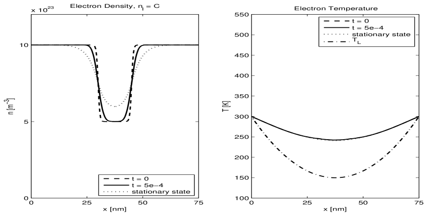
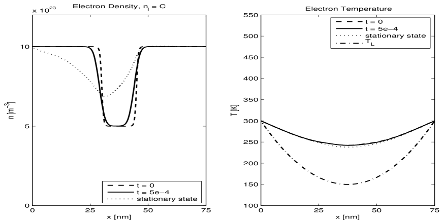
Figure 1. Electron density and temperature in the ballistic diode with cooling lattice temperature at voltages $U=0.2$ V (top) and $U=1.0$ V (bottom).

Figure 2 illustrates the behavior of the electron density and electron temperature when the lattice temperature is heating the diode, i.e. $\theta_{L}(x)=\frac{7}{4}-3(x-\frac{1}{2})^{2}$. Again, the electron temperature converges to a nonhomogeneous steady state, and the behavior of the particle density is similar to the case of cooling temperatures. The current-voltage characteristic is very close to that one with constant temperature (not presented). It can be seen that only for very large voltages, the current density becomes slightly smaller due to an increasing thermal energy fraction. This shows that the influence of the temperature equation is not very important in a ballistic diode although there are significant temperature gradients.

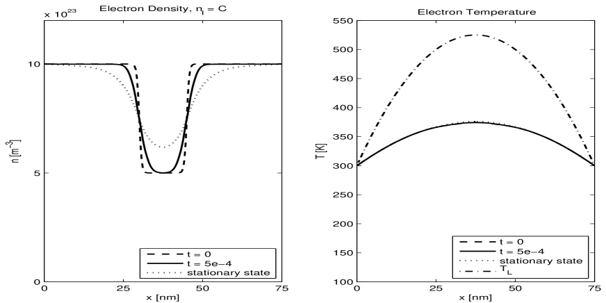
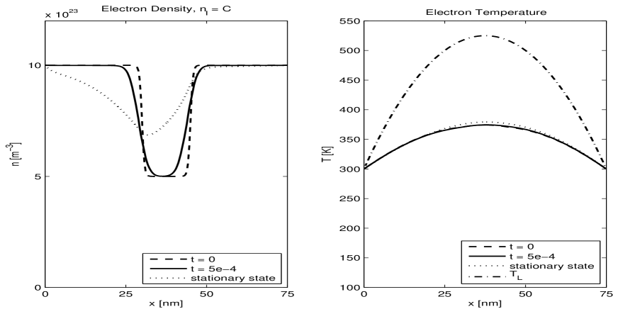
Figure 2. Electron density and temperature in the ballistic diode with heating lattice temperature at voltages $U=0.2$ V (top) and $U=1.0$ V (bottom).