Trap anharmonicity and sloshing mode of a Fermi gas

Abstract

For a gas trapped in a harmonic potential, the sloshing (or Kohn) mode is undamped and its frequency coincides with the trap frequency, independently of the statistics, interaction and temperature of the gas. However, experimental trap potentials have usually Gaussian shape and anharmonicity effects appear as the temperature and, in the case of Fermions, the filling of the trap are increased. We study the sloshing mode of a degenerate Fermi gas in an anharmonic trap within the Boltzmann equation, including in-medium effects in both the transport and collision terms. The calculated frequency shifts and damping rates of the sloshing mode due to the trap anharmonicity are in satisfactory agreement with the available experimental data. We also discuss higher-order dipole, octupole, and bending modes and show that the damping of the sloshing mode is caused by its coupling to these modes.

I Introduction

In a couple of experiments, the measurement of the frequencies of collective modes in trapped Fermi gases revealed a lot of interesting information on the equation of state, the validity of superfluid hydrodynamics, and the superfluid-normal phase transition KinastHemmer2004 ; BartensteinAltmeyer2004 ; KinastTurlapov2004 ; AltmeyerRiedl2007a ; AltmeyerRiedl2007b . More recently, the transition from the hydrodynamic to the collisionless regime in the normal phase was also studied Wright2007 ; Riedl2008 . However, since the frequencies of the collective modes depend on the trap frequencies, a precise knowledge of the latter is required for a meaningful interpretation of the collective-mode data.

A possibility to determine the trap frequency with high precision is the measurement of the frequency of the sloshing mode AltmeyerRiedl2007a , which is an oscillation of the center of mass of the trapped atom cloud. In a harmonic trap, this oscillation (also called Kohn mode) is undamped and its frequency coincides exactly with the trap frequency in the corresponding direction, independently of the number of atoms $N$, or their interaction, their temperature $T$ etc. This is a consequence of the Kohn theorem Kohn ; Brey and follows from the fact that the center-of-mass oscillation decouples completely from the internal dynamics of the gas if the interaction is translationally invariant and the external potential is harmonic Dobson .

However, in practice the trap potential is never exactly harmonic. In optical dipole traps GrimmWeidemueller00 , the potential is typically Gaussian (corresponding to the intensity profile of the laser beam). Because of this anharmonicity, the frequency of the sloshing mode is shifted, and the shift depends on the system parameters such as $N$, $T$, the scattering length $a$ characterizing the interaction strength, etc. Furthermore, the sloshing mode is no longer undamped.

The anharmonicity of the trap complicates considerably the analysis of collective-mode experiments. In LABEL:Riedl2008 the measured frequencies were corrected for the anharmonicity effects by giving them in units of the measured frequency of the sloshing mode. However, it is clear that the damping rates of the modes cannot be corrected in this way. In LABEL:WuZhang2012_2d, the damping rate of the sloshing mode was used to estimate the increase of the damping rate of other modes due to the anharmonicity. Both corrections are ad-hoc prescriptions without rigorous justification. It is therefore strongly desirable to get a better understanding of the anharmonicity effects on the sloshing mode.

The aim of the present paper is to describe theoretically the frequency shift and the damping rate of the sloshing mode in an anharmonic trap. We will compare our results with the experimental data available from the Innsbruck group Riedl2008 ; Sidorenkov2012 and with the numerical results by Wu and Zhang WuZhang2012_3d . We will also discuss in detail the damping mechanism of the sloshing mode. In an anharmonic potential, the center-of-mass motion is no longer decoupled from the internal degrees of freedom of the cloud. We will see that the damping of the transverse sloshing mode is a consequence of its coupling to other damped collective modes, in particular to the radial dipole mode and the bending mode.

The framework of our study is the Boltzmann equation, including mean field Chiacchiera2009 and in-medium cross-section BruunSmith2007 ; Riedl2008 ; Chiacchiera2009 . Especially the mean field is expected to be important in the present context, because it can have a sizable effect on the density profile, i.e., on how far the cloud extends into the anharmonic region of the trap potential. The Boltzmann equation is solved approximately with the help of the phase-space moments method. This method, when extended beyond the lowest order, has proven to be in very good quantitative agreement with the results of a full numerical simulation Lepers2010 . It has also been quite successful for the description of the experimental results for the frequency and damping rate of the radial quadrupole mode Chiacchiera2011 . In the present case of the sloshing mode, we include phase-space moments of first and third order.

The paper is organized as follows. The general formalism is briefly presented in Sec. II. Then we specify our model for the experimental trap potential in Sec. III. In Sec. IV, we give a formula for the frequency shift of the sloshing mode within the first-order moments method. Then we extend the ansatz to third order in Sec. V. The physical contents of the extended ansatz and the numerical results are discussed. In Sec. VI the third-order ansatz is used to describe also the radial dipole, radial octupole, and bending modes. Finally, in Sec. VII, we will conclude.

Throughout the paper, we use units with $\hbar=k_{B}=1$.

II Summary of the formalism

In this section, we give a short summary of the formalisms of Refs. Chiacchiera2009 ; Chiacchiera2011 . More details can be found there.

II.1 Linearized Boltzmann equation with in-medium effects

We consider a balanced two-component ($N_{\uparrow}=N_{\downarrow}=N/2$) Fermi gas of atoms with mass $m$ and interspecies attractive interaction (scattering length $a<0$), trapped in a potential $V_{T}(\bm{\mathrm{r}})$. The framework we use to describe the collective dynamics of the system in the normal-fluid phase is the Boltzmann equation. We assume that the two components move in phase, so that only one distribution function $f=f_{\uparrow}=f_{\downarrow}$ is needed. It is normalized to $\int d^{3}rd^{3}p/(2\pi)^{3}f=N/2$, and expectation values of one-body operators are given by

$$\langle q\rangle(t)=\frac{2}{N}\int\frac{d^{3}rd^{3}p}{(2\pi)^{3}}f(\bm{\mathrm{r}},\bm{\mathrm{p}},t)q(\bm{\mathrm{r}},\bm{\mathrm{p}})\,.$$ (1)

As in LABEL:Chiacchiera2009, we include in-medium effects in both the transport and the collision parts of the Boltzmann equation: a mean field like potential $U$ and the in-medium modified cross-section $d\sigma/d\Omega$, respectively.

Within the Thomas-Fermi or local-density approximation (LDA), the equilibrium distribution function reads

$$f_{\mathit{eq}}(\bm{\mathrm{r}},\bm{\mathrm{p}})=\frac{1}{e^{\beta[\frac{\bm{\mathrm{p}}^{2}}{2m}+V_{T}(\bm{\mathrm{r}})+U_{\mathit{eq}}(\bm{\mathrm{r}})-\mu_{0}]}+1},$$ (2)

where $U_{\mathit{eq}}$ is the mean field in equilibrium, $\mu_{0}$ is the chemical potential, and $\beta=1/T$ is the inverse temperature. As in LABEL:Chiacchiera2009, we obtain $U_{\mathit{eq}}$ from the single-particle self-energy in ladder approximation, evaluated at the Fermi level. In the weak coupling limit, this reduces to the Hartree term $U_{\mathrm{Hartree}}=4\pi a\rho/m$, where $\rho=\int d^{3}p/(2\pi)^{3}f$ is the density per spin state, and it remains finite for all interaction strengths up to the unitary limit, $a\to-\infty$. In equilibrium, the main effect of the mean field is to enhance the density in the center of the trap, as shown in Fig. 3 of LABEL:Chiacchiera2009.

For the study of collective oscillations, it is sufficient to consider small deviations from equilibrium and to linearize the Boltzmann equation with respect to $\delta f=f-f_{\mathit{eq}}$. If we write the variation of the distribution function in the form Landau10

$$\delta f(\bm{\mathrm{r}},\bm{\mathrm{p}},t)=f_{\mathit{eq}}\bar{f}_{\mathit{eq}}\Phi(\bm{\mathrm{r}},\bm{\mathrm{p}},t)\,,$$ (3)

with $\bar{f}_{\mathit{eq}}=1-f_{\mathit{eq}}$, the linearized Boltzmann equation can be written as

$$f_{\mathit{eq}}\bar{f}_{\mathit{eq}}\Big{(}\dot{\Phi}+\Big{\{}\Phi,\frac{p^{2}}{2m}+V_{T}+U_{\mathit{eq}}\Big{\}}\\ +\beta\frac{\bm{\mathrm{p}}}{m}\cdot\bm{\nabla}_{r}(\delta V+\delta U)\Big{)}=-I[\Phi]\,,$$ (4)

where $\{F,G\}=\bm{\nabla}_{r}F\cdot\bm{\nabla}_{p}G-\bm{\nabla}_{p}F\cdot\bm{\nabla}_{r}G$ denotes the Poisson bracket, $\delta V$ is the perturbation of the trap potential that is used to excite the collective mode, $\delta U$ is the variation of the mean field due to the variation of the density, and $I[\Phi]$ is the linearized collision term. Since we want to calculate the so-called response function, we take the perturbation to be a pulse,

$$\delta V(\bm{\mathrm{r}},t)=\hat{V}(\bm{\mathrm{r}})\delta(t)\,.$$ (5)

As in LABEL:Chiacchiera2009, we approximate the variation of the mean field by

$$\delta U(\bm{\mathrm{r}},t)=\left.\frac{\partial U_{\mathit{eq}}}{\partial\rho_{\mathit{eq}}}\right|_{\rho_{\mathit{eq}}(\bm{\mathrm{r}}),T}\,\delta\rho(\bm{\mathrm{r}},t)\,.$$ (6)

The linearized collision integral reads

$$I[\Phi]=\int\frac{d^{3}p_{1}}{(2\pi)^{3}}\int d\Omega\,\frac{d\sigma}{d\Omega}\frac{|\bm{\mathrm{p}}-\bm{\mathrm{p}}_{1}|}{m}f_{\mathit{eq}}f_{\mathit{eq}1}\bar{f}_{\mathit{eq}}^{\prime}\bar{f}_{\mathit{eq}1}^{\prime}\\ \times(\Phi+\Phi_{1}-\Phi^{\prime}-\Phi_{1}^{\prime})\,,$$ (7)

where an obvious notation for the different $f_{\mathit{eq}}$ and $\Phi$ at the momenta before ($\bm{\mathrm{p}}$, $\bm{\mathrm{p}}_{1}$) and after the collision ($\bm{\mathrm{p}}^{\prime}$, $\bm{\mathrm{p}}_{1}^{\prime}$) has been used. Note that, especially near the critical temperature, the in-medium cross-section $d\sigma/d\Omega$ can differ strongly from the free one BruunSmith2007 ; Riedl2008 ; Chiacchiera2009 .

II.2 Moments method

As in LABEL:Chiacchiera2011, we are looking for a semi-analytical solution of the Boltzmann equation (4) by using the method of phase-space moments. In this section, we will generalize the formalism of that paper to the case of an arbitrary trap potential $V_{T}$ and with mean field $U$.

The basic idea is to approximate the function $\Phi$ by a polynomial in the components of $\bm{\mathrm{r}}$ and $\bm{\mathrm{p}}$ with time-dependent coefficients $c_{j}$,

$$\Phi(\bm{\mathrm{r}},\bm{\mathrm{p}},t)=\sum_{j=1}^{n}c_{j}(t)\phi_{j}(\bm{\mathrm{r}},\bm{\mathrm{p}})\,,$$ (8)

where the $\phi_{j}$ are suitable basis functions, e.g., monomials in the components of $\bm{\mathrm{r}}$ and $\bm{\mathrm{p}}$.

Multiplying the linearized Boltzmann equation (4) by $\phi_{i}$ and integrating over phase space, one obtains, after a Fourier transform with respect to $t$, a set of $n$ coupled linear algebraic equations for the $n$ coefficients $c_{j}(\omega)$. In matrix form, they read

$$\sum_{j=1}^{n}A_{ij}(\omega)c_{j}(\omega)=a_{i}\,,$$ (9)

where

$$A_{ij}(\omega)=-i\omega M_{ij}+A^{\mathit{trans}}_{ij}+A^{{\delta U}}_{ij}+A^{\mathit{coll}}_{ij}\,,$$ (10)

$$M_{ij}=\int\frac{d^{3}rd^{3}p}{(2\pi)^{3}}f_{\mathit{eq}}\bar{f}_{\mathit{eq}}\phi_{i}\phi_{j}\,,$$ (11)

$$A^{\mathit{trans}}_{ij}=-\frac{N}{2\beta}\langle\{\phi_{i},\phi_{j}\}\rangle_{\mathit{eq}}\,,$$ (12)

$$A^{{\delta U}}_{ij}=\frac{N}{2}\langle\bm{\nabla}_{p}\phi_{i}\cdot\bm{\nabla}_{r}\delta U_{j}\rangle_{\mathit{eq}}\,,$$ (13)

$$A^{\mathit{coll}}_{ij}=\int\frac{d^{3}rd^{3}p}{(2\pi)^{3}}\phi_{i}I[\phi_{j}]\,,$$ (14)

and

$$a_{i}=-\frac{N}{2}\langle\bm{\nabla}_{p}\phi_{i}\cdot\bm{\nabla}_{r}\hat{V}(\bm{\mathrm{r}})\rangle_{\mathit{eq}}\,.$$ (15)

The variation of the mean field in Eq. (13) is defined as

$$\delta U_{j}=\frac{\partial U_{\mathit{eq}}}{\partial\rho_{\mathit{eq}}}\int\frac{d^{3}p}{(2\pi)^{3}}f_{\mathit{eq}}\bar{f}_{\mathit{eq}}\phi_{j}\,,$$ (16)

Equations (12) and (15) correspond to Eqs. (14) and (16) in LABEL:Chiacchiera2011 which have been simplified by integration by parts. Comparing Eqs. (9)-(15) with the analogous ones of LABEL:Chiacchiera2011, Eqs. (11)-(16), one sees that the mean field gives rise to a new term, $A^{\delta U}$. However, one should keep in mind that implicitly all terms depend on the mean field since it modifies the equilibrium distribution $f_{\mathit{eq}}$. One can see that the matrices $M$ and $A^{\mathit{coll}}$ are symmetric, $A^{\mathit{trans}}$ is antisymmetric, whereas $A^{\delta U}$ has no defined symmetry. In practice, the calculation of the matrices is straight-forward, but tedious, and we made use of the Mathematica software to express the numerous matrix elements in terms of a smaller number of integrals over equilibrium quantities.

II.3 Eigenmodes and response function

Without an external perturbation $\hat{V}$, i.e., for $a_{i}=0$, Eq. (9) has a solution with non-vanishing coefficients $c_{j}$ only if $\det A(\omega)=0$. The frequencies $\omega$ for which this happens are obviously given by the eigenvalues of the matrix $-iM^{-1}(A^{\mathit{trans}}+A^{\delta U}+A^{\mathit{coll}})$. If they are well separated, it is possible to interpret them as the frequencies of the eigenmodes of the system. In general, they are complex, and their imaginary part describes the damping rate of the corresponding mode Riedl2008 ; Chiacchiera2009 .

However, as discussed in LABEL:Chiacchiera2011, when the moments method is extended to higher order, there can be many eigenvalues belonging to a single collective mode. In this case, the scattering of the eigenvalues, which goes over into a continuous spectrum in the limit of an infinite number of moments DaProvidencia1988 , corresponds to a new contribution to the damping (Landau damping) in addition to the imaginary parts coming from the collision term. In order to obtain the mode frequency and damping rate in this case, it is useful to look at the response function which contains the contributions of all eigenvalues.

We denote by $\langle q\rangle(\omega)$ the Fourier transform of the expectation value $\langle q\rangle(t)$ of some operator $q$ after the perturbation. The so-called response function is equal to $\delta\langle q\rangle(\omega)/\alpha\equiv(\langle q\rangle(\omega)-\langle q\rangle_{eq})/\alpha$ in the special case that the excitation operator is $\hat{V}=\alpha q$. In all excitations considered in this paper, $\langle q\rangle_{eq}$ will be zero. The strength function is proportional to the imaginary part of the response function.

In order to calculate the response function, we need the coefficients $c_{j}(\omega)$ of the ansatz (8). By diagonalizing the matrix

$$M^{-1}(A^{\mathit{trans}}+A^{\delta U}+A^{\mathit{coll}})=PDP^{-1}\,,$$ (17)

with $D=\textrm{diag}(\Gamma_{1}+i\omega_{1},\dots,\Gamma_{n}+i\omega_{n})$, we can write them as

$$c_{j}(\omega)=i\sum_{k=1}^{n}\frac{P_{jk}(P^{-1}M^{-1}a)_{k}}{\omega-\omega_{k}+i\Gamma_{k}}\,.$$ (18)

Then, the response function can be easily obtained as $\langle q\rangle(\omega)=b^{T}c(\omega)$, where

$$b_{i}=\frac{2}{N}\int\frac{d^{3}rd^{3}p}{(2\pi)^{3}}f_{\mathit{eq}}\bar{f}_{\mathit{eq}}q\phi_{i}\,.$$ (19)

The frequency and damping of the mode can be extracted from the response $\langle q\rangle(\omega)$, e.g., by fitting the peak in the strength function $-\operatorname{Im}\langle q\rangle(\omega)$ corresponding to the mode under consideration with a Lorentzian.

Using the solution for the coefficients $c_{j}(\omega)$ at the peak, we can also obtain the velocity field of the corresponding collective mode:

$$\bm{\mathrm{v}}(\bm{\mathrm{r}},\omega)=\sum_{j=1}^{n}c_{j}(\omega)\frac{1}{\beta\rho_{\mathit{eq}}}\int\frac{d^{3}p}{(2\pi)^{3}}f_{\mathit{eq}}\bm{\nabla}_{p}\phi_{j}\,.$$ (20)

III Realistic trap potential

In this section we recall the shape of a typical optical dipole trap. We concentrate on the configuration used by the Innsbruck group, consisting of a focused-beam trap GrimmWeidemueller00 with additional magnetic confinement in the axial direction. Following LABEL:Altmeyer_Thesis, we parametrize the experimental trap potential as

$$V_{\mathit{exp}}(\bm{\mathrm{r}})=V_{0}\left[1-\frac{1}{1+\frac{z^{2}}{z_{0}^{2}}}\exp\left(-\frac{2}{1+\frac{z^{2}}{z_{0}^{2}}}\frac{r_{\perp}^{2}}{w_{0}^{2}}\right)\right]\\ +\frac{1}{2}m\omega_{z,\mathit{mag}}^{2}z^{2}\,,$$ (21)

where $r_{\perp}=\sqrt{x^{2}+y^{2}}$, $V_{0}$ is the trap depth, $w_{0}$ is the minimal waist of the laser beam, $z_{0}=\pi w_{0}^{2}/\lambda$ is the Rayleigh length, $\lambda$ the laser wavelength and $\omega_{z,\mathit{mag}}$ defines the magnetic trapping in the $z$ direction.

In order to compare our results with the data from Refs. Riedl2008 ; Sidorenkov2012 , we focus on the setup of that experiment. The trap was of the type (21), with strong anharmonicity in the $x$-$y$ plane due to the Gaussian shape of the laser beams. The confinement along the $z$ direction was practically harmonic. In our calculations, we will expand Eq. (21) up to second order in $z$ and up to sixth order in $r_{\perp}$. The result can be written as

$$V_{\mathit{6th}}(\bm{\mathrm{r}})=\frac{m\omega_{\perp}^{2}r_{\perp}^{2}}{2}\Big{(}1-\frac{m\omega_{\perp}^{2}r_{\perp}^{2}}{4V_{0}}+\frac{m^{2}\omega_{\perp}^{4}r_{\perp}^{4}}{24V_{0}^{2}}\Big{)}\\ +\frac{m\omega_{z}^{2}z^{2}}{2}\,,$$ (22)

where $\omega_{\perp}^{2}=4V_{0}/(mw_{0}^{2})$ and $\omega_{z}^{2}=\omega_{z,\mathit{mag}}^{2}+\omega_{z,\mathit{opt}}^{2}=\omega_{z,\mathit{mag}}^{2}+2V_{0}/(mz_{0}^{2})$ are the radial and axial trap frequencies, respectively. We use Eq. (22) instead of Eq. (21) because it simplifies the calculations in the sense that it leads to a density that tends to zero for $r_{\perp}\to\infty$. The necessity to go beyond fourth order is also clear from Eq. (22): otherwise the potential would be unbound from below. For illustration, Fig. 1

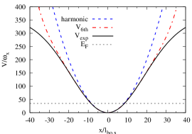
Figure 1: Experimental trap potential (solid line), and its harmonic (dashes) and sixth-order approximation (dash-dotted line), as functions of $x$ for $y=z=0$. The Fermi energy for the parameters of LABEL:Riedl2008 is indicated by the thin dashes. The potentials are in units of $\omega_{x}$ and $x$ is in units $l_{ho,x}=1/\sqrt{m\omega_{x}}$.

shows the real trap potential (21), its harmonic approximation, and the one we will use, Eq. (22).

In the present paper, we concentrate on axially symmetric traps. Nevertheless, we write $\omega_{x}$ and $\omega_{y}$ instead of $\omega_{\perp}$ for the trap frequencies in $x$ and $y$ direction if the formulas can be generalized to the triaxial case.

In our numerical calculations, we use as an example the parameters of the Innsbruck experiment Riedl2008 . As mentioned in LABEL:Riedl2008, the sloshing mode was studied with the same parameters as the compression mode, i.e., $\omega_{\perp}/(2\pi)=1100$ Hz, $\omega_{z}/(2\pi)=26$ Hz, and $V_{0}=19$ $\mu$K. The trap was loaded with $N=6\times 10^{5}$ atoms of ⁶Li in the unitary limit, $1/(k_{F}a)=0$, and the temperature was varied between $\sim 0$ and $1.2T_{F}$. Since we cannot describe the superfluid phase, we limit ourselves to temperatures above $0.3T_{F}$ Chiacchiera2009 . Moreover, we approximate the unitary limit numerically by setting $1/(k_{F}a)=-0.01$.

As pointed out in LABEL:Riedl2008, the anharmonicity effects depend mainly upon the ratio $E_{F}/V_{0}$. Defining the Fermi energy as usual by $E_{F}=(3N\omega_{\perp}^{2}\omega_{z})^{1/3}$, one obtains $E_{F}/V_{0}\approx 0.1$, i.e., at low temperature the anharmonicity effects are relatively weak. For illustration, $E_{F}$ is indicated in Fig. 1 by the thin dashed line. We see that, for the present choice of parameters, the atoms start to feel the anharmonicity of the potential when their energy exceeds $E_{F}$, while the sixth-order approximation to the potential stays very precise up to about five times the Fermi energy.

IV Sloshing mode at first order

In order to describe the sloshing motion, say, along the $x$ direction, the ansatz (8) has to contain at least two basis functions:

$$\Phi_{\mathit{1st}}(\bm{\mathrm{r}},\bm{\mathrm{p}},t)=c_{1}(t)x+c_{2}(t)p_{x}\,.$$ (23)

The second term describes the collective velocity of the cloud in $x$ direction, while the first one corresponds approximately to a displacement of the center of mass. The latter statement becomes exact in the special case of a purely harmonic trap without mean field ($U=0$). In this case, the ansatz (23) is closed with respect to the operator $\bm{\mathrm{p}}/m\cdot\bm{\nabla}_{r}-\bm{\nabla}_{r}V_{T}\cdot\bm{\nabla}_{p}$ on the left-hand side of the Boltzmann equation (4), and since the collision term does not contribute ($I[x]=I[p_{x}]=0$ because of momentum conservation in a collision), the ansatz (23) becomes exact. However, if the trap is not purely harmonic, this is no longer true, since the gradient of the trap potential generates new terms. And even if the trap is harmonic, it is not true for interacting atoms, which feel a mean field $U\neq 0$ in addition to the trap potential $V_{T}$. In the next section, we will therefore extend the ansatz (23), but let us first look what happens at first order.

We now apply the formalism described in Sec. II to $\Phi_{\mathit{1st}}$. The calculation of the matrix $A$ is very easy in this case. After some algebra, we obtain a quadratic equation for the frequency of the sloshing mode by imposing $\det A=0$. Its solution reads

$$\omega_{\mathit{slosh}}^{2}=\frac{1-C}{1-C-C^{\prime}}\omega_{x}^{2}\,.$$ (24)

The parameters

$$C=\frac{2\beta}{N}\int\frac{d^{3}rd^{3}p}{(2\pi)^{3}}\,f_{\mathit{eq}}\bar{f}_{\mathit{eq}}x\frac{\partial U_{\mathit{eq}}}{\partial x}$$ (25)

and

$$C^{\prime}=-\frac{2\beta}{N}\int\frac{d^{3}rd^{3}p}{(2\pi)^{3}}f_{\mathit{eq}}\bar{f}_{\mathit{eq}}x\frac{\partial}{\partial x}\Big{(}\frac{m\omega_{x}^{2}x^{2}}{2}-V_{T}(\bm{\mathrm{r}})\Big{)}$$ (26)

characterize, respectively, the strength of the mean field and of the anharmonicity effects. Equation (24) has two important features: (a) If $V_{T}$ is harmonic ($C^{\prime}=0$), then $\omega_{\mathit{slosh}}=\omega_{x}$, independently of the interaction, in accordance with the Kohn theorem Kohn . This point was already discussed in LABEL:Chiacchiera2009 and shows the consistency of our approach, in particular of Eq. (6). (b) If $V_{T}$ is not purely harmonic ($C^{\prime}\neq 0$), then $\omega_{\mathit{slosh}}$ depends on both the anharmonicity of the trap and on the interaction.

Another property of Eq. (24) is that the sloshing mode is undamped (i.e., $\omega_{\mathit{slosh}}$ is real) even in the case of an anharmonic potential. This is, however, only a consequence of the first-order approximation.

A similar calculation was performed in the Appendix B of LABEL:Riedl2008. In that reference, only the leading anharmonicity correction was kept. If we combine Eqs. (22), (24), and (26) and keep only the leading order in $1/V_{0}$, we find

$$\omega_{\mathit{slosh}}^{2}=\omega_{x}^{2}\Big{(}1-\frac{m\omega_{\perp}^{2}(3\langle x^{2}\rangle_{\mathit{eq}}+\langle y^{2}\rangle_{\mathit{eq}})}{2V_{0}(1-C)}\Big{)}\,.$$ (27)

This result differs from Eq. (B2) of LABEL:Riedl2008 in two respects. First, there is an additional factor of three in front of the $\langle x^{2}\rangle$ term (misprint in LABEL:Riedl2008). Second, the anharmonicity correction is enhanced by a factor $1/(1-C)$. This factor is missing in LABEL:Riedl2008 because there the mean field was not considered, although the expectation values $\langle x^{2}\rangle$ and $\langle y^{2}\rangle$ were calculated with the density profiles of an interacting gas.

V Sloshing mode at third order

V.1 Extended ansatz

As in LABEL:Chiacchiera2011, we will extend the ansatz (23) by including higher-order terms. At the next higher order, the ansatz contains 18 terms

$$\Phi_{\mathit{3rd}}(\bm{\mathrm{r}},\bm{\mathrm{p}},t)=\sum_{i=1}^{18}c_{i}(t)\phi_{i}(\bm{\mathrm{r}},\bm{\mathrm{p}})\,,$$ (28)

where:

$$\phi_{1}=x\,,\,\phi_{2}=p_{x}\,,$$

$$\phi_{3}=x^{3}\,,\,\phi_{4}=x^{2}p_{x}\,,\,\phi_{5}=xp_{x}^{2}\,,\,\phi_{6}=p_{x}^{3}\,,$$

$$\phi_{7}=xy^{2}\,,\phi_{8}=y^{2}p_{x}\,,\,\phi_{9}=xyp_{y}\,,\,\phi_{10}=yp_{x}p_{y}\,$$

$$\phi_{11}=xp_{y}^{2}\,,\,\phi_{12}=p_{x}p_{y}^{2}\,,\,\phi_{13}=xz^{2}\,,\,\phi_{14}=z^{2}p_{x}\,,$$

$$\phi_{15}=xzp_{z}\,,\,\phi_{16}=zp_{x}p_{z}\,,\,\phi_{17}=xp_{z}^{2}\,,\,\phi_{18}=p_{x}p_{z}^{2}.$$ (29)

The first two terms of $\Phi_{\mathit{3rd}}$ coincide with $\Phi_{\mathit{1st}}$, and the subsequent ones are all possible terms of third order in the components of $\bm{\mathrm{r}}$ and $\bm{\mathrm{p}}$ satisfying the symmetries of the mode: odd under $(x,p_{x})\to(-x,-p_{x})$ and even under $(y,p_{y})\to(-y,-p_{y})$ and $(z,p_{z})\to(-z,-p_{z})$.

Note that some of the third-order terms, e.g., $\phi_{4}=x^{2}p_{x}$, generate a velocity field that is quadratic in the coordinates, whereas the velocity field corresponding to the first-order ansatz is spatially constant. Other terms, e.g., $\phi_{5}=xp_{x}^{2}$ or $\phi_{6}=p_{x}^{3}$, describe momentum-sphere distortions. They give rise to a non-vanishing collision integral so that they generate a damping. The momentum-independent third-order terms such as $\phi_{3}=x^{3}$ describe deformations of the cloud in coordinate space that will be discussed in more detail in the next subsection.

As explained in Sec. II.3, the frequency and damping rate should now be extracted from the response function. The suitable excitation operator is

$$\hat{V}_{\mathit{slosh}}(\bm{\mathrm{r}})=\alpha x\,,$$ (30)

because it gives all atoms a constant kick in $x$ direction, $p_{x}\to p_{x}-\alpha$, at the moment of the excitation $t=0$. The response function is defined as the expectation value $\langle x\rangle(\omega)/\alpha$.

We checked numerically that, in a purely harmonic potential $(V_{0}\to\infty)$, the strength function has only a single sharp peak (no damping) at $\omega=\omega_{x}$ within the precision of our calculation (better than $10^{-4}$), independently of the temperature and of the interaction strength.

In Fig. 2

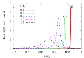
Figure 2: Strength function $-\operatorname{Im}\langle x\rangle(\omega)$ for the sloshing mode (excitation $\hat{V}=\alpha x$) in the anharmonic trap for various temperatures. The system parameters are those of LABEL:Riedl2008.

we show the strength functions for the sloshing mode in the anharmonic trap for various temperatures. In all cases the strength is concentrated in a single peak and the width of the peak corresponds to the damping rate. The position of the peak is always below $\omega=\omega_{x}$, and with increasing temperature, this shift gets stronger. This is easily understood: With increasing temperature, more and more atoms reach the peripheral region where the anharmonic potential is flatter than the harmonic one (cf. Fig. 1).

Since in all the cases shown in Fig. 2 the strength is concentrated in a single peak, this allows us to extract the frequency and damping rate by fitting it with a single Lorentzian. (This is not clear a priori: For instance, if we do the calculation without mean field, the strength function for low temperature has two separate peaks, and it is not evident how one has to define the average frequency and total width.) The results for the frequency and damping rate as functions of temperature are shown in Fig. 3(a)

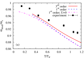
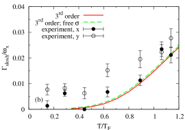
Figure 3: (a) Temperature dependence of the frequency of the transverse sloshing mode in units of $\omega_{x}$. Solid line: third-order result; dashed line: first-order result; dash-dotted line: first-order result obtained without mean field. The experimental data points are taken from LABEL:Riedl2008. (b) Temperature dependence of the damping rate in units of $\omega_{x}$. Solid line: full third-order result; dashed line: third-order result obtained with the free instead of the in-medium cross section. The filled and empty data points are measured damping rates of the sloshing modes in $x$ and $y$ direction, respectively, from LABEL:Sidorenkov2012.

and (b) as the solid lines. For comparison, the dashed line in Fig. 3(a) shows the first-order result for the frequency. The dash-dotted line corresponds to the first-order result obtained without mean field. As expected, the mean field reduces the shift of the frequency, but its effect is moderate and most pronounced at lower temperature.

The experimental results from Fig. 2 of LABEL:Riedl2008 are also shown in Fig. 3(a). In that paper, the measured empirical temperatures $\tilde{T}$ were already converted into real temperatures $T/T_{F}$ as explained in Kinast2005 ; Chen2005 , so that the results can immediately be compared with our calculation. The trend is correctly reproduced, and the third-order result is clearly in better agreement with the data than the first-order one, but the theoretical frequency shift is still stronger than the experimental shifts reported in LABEL:Riedl2008. However, one should keep in mind that while $\omega_{\mathit{slosh}}$ was precisely determined, the ratio $\omega_{\mathit{slosh}}/\omega_{x}$ depends also on $\omega_{x}$, which was not very well known in that experiment. Actually, $\omega_{x}$ was deduced from $\omega_{\mathit{slosh}}$ under the assumption that the anharmonicity effects become negligible at $T=0$ Sidorenkov2012 . If we suppose that the true trap frequency $\omega_{x}$ was just $\sim 1.5$% higher, the data points for $\omega_{\mathit{slosh}}/\omega_{x}$ are slightly shifted downwards and the agreement between theory and data becomes much better.

The damping rate, shown in Fig. 3(b), increases strongly with the temperature: at $T/T_{F}=0.4$ the sloshing mode survives for several hundreds of oscillation periods, whereas at $T/T_{F}=1.2$ its amplitude decreases by a factor of $1/e$ after $\sim 6$ oscillations. The in-medium modification of the cross-section has only a small effect on the damping of the sloshing mode. The experimental data from LABEL:Sidorenkov2012 are in quite good agreement with our theoretical result, especially at the high temperature. The strongly scattered damping rates at low temperature are probably an artefact due to a beat caused by the small residual ellipticity of the trap potential in the experiment.

We also compared our results with those shown in Fig. 5(a) of the recent paper WuZhang2012_3d by Wu and Zhang, where they solve the Boltzmann equation numerically within the relaxation-time approximation with a local relaxation time $\tau(\bm{\mathrm{r}})$ taken from LABEL:MassignanBruun2005. As we discussed in our previous work Lepers2010 ; Chiacchiera2011 , the inclusion of higher-order moments accounts in an approximate way for the spatial dependence of the relaxation time. For the sake of comparison, we use the same trap parameters as Wu and Zhang, namely, $\omega_{\perp}/(2\pi)=1800$ Hz, $\omega_{z}/(2\pi)=32$ Hz, and $V_{0}=50$ $\mu$K, and neglect, as it is done in LABEL:WuZhang2012_3d, the mean field and in-medium effects on the cross section. Because of the larger trap depth, the frequency shifts are somewhat weaker than those shown in Fig. 3(a). Since in the calculation by Wu and Zhang the frequency depends on the oscillation amplitude, we have to compare with the results obtained for the smallest amplitude [red squares in Fig. 5(a) of LABEL:WuZhang2012_3d]. If we extrapolate these results, shown only up to $T/T_{F}=0.4$ in LABEL:WuZhang2012_3d, to higher temperatures, they are in quite good agreement with our results above $T/T_{F}\sim 0.5$. At lower temperatures, however, our frequency shift is slightly stronger than that by Wu and Zhang, probably because they use Boltzmann instead of Fermi distributions so that their density is more concentrated in the trap center at low temperatures.

V.2 Coupling between sloshing and other modes

In a harmonic trap, a characteristic feature of the Kohn mode Kohn is that, as long as the interaction is translationally invariant, the cloud moves as a whole without any change in size or shape Dobson , as illustrated in Figs. 4(a)

Figure 4: Schematic representation of the oscillation of the density profile in $x$ direction ($\rho_{x}$ being the density integrated over $y$ and $z$) for (a) the Kohn mode, in which the cloud oscillates as a whole, and (b) the radial compressional dipole mode, where the cloud shape oscillates, while the center of mass of the cloud stays at rest. All density profiles have the same normalization (number of atoms) and the same width.

and 5(a).

Figure 5: Schematic representation of (a) the Kohn mode, in which the cloud oscillates as a whole, and (b) the bending mode, where the cloud shape oscillates, while the center of mass of the cloud stays at rest.

In an anharmonic trap, this is no longer the case and the cloud will be slightly distorted during the oscillation. In other words, because of the anharmonicity, the pure center-of-mass motion gets coupled to other collective modes. These are damped as usual by collisions, which results in a damping of the sloshing mode.

What kind of distortions of the cloud shape can one expect? Let us first note that, to first order in the perturbation, the cloud width cannot be changed (neither in the transverse nor in the axial direction), because the excitation operator is odd with respect to $x\leftrightarrow-x$.

However, the density profile can become skewed in the direction of the oscillation (i.e., in the $x$ direction in our case). For illustration, Fig. 4(b) shows how the density profile changes during a radial compressional dipole oscillation. To derive the corresponding operator, let us start from the usual definition of the skewness, which is proportional to $\langle(x-\langle x\rangle)^{3}\rangle$. Keeping only terms linear in the variations $\delta\langle x\rangle$ and $\delta\langle x^{2}\rangle$, and using $\langle x\rangle_{\mathit{eq}}=0$, we find that for small oscillations, this is equal to $\langle x^{3}-3\langle x^{2}\rangle_{\mathit{eq}}x\rangle$. If the trap is axially symmetric, collective modes of different multipolarity in the radial direction do not mix. It is therefore useful to decompose the operator into dipolar and octupolar parts: $x^{3}-3\langle x^{2}\rangle_{\mathit{eq}}x=\frac{3}{4}q_{\mathit{dip}}+\frac{1}{4}q_{\mathit{oct}}$ with

$$q_{\mathit{dip}}=(r_{\perp}^{2}-2\langle r_{\perp}^{2}\rangle_{\mathit{eq}})r_{\perp}\cos\varphi=(x^{2}+y^{2}-2\langle r_{\perp}^{2}\rangle_{\mathit{eq}})x\,,$$ (31)

$$q_{\mathit{oct}}=r_{\perp}^{3}\cos 3\varphi=(x^{2}-3y^{2})x\,.$$ (32)

Only $q_{\mathit{dip}}$ can get a non-vanishing expectation value during the sloshing oscillation.

Another possible distortion involves the axial ($z$) direction. Let us consider again the sloshing mode in $x$ direction. Then one could imagine that the cloud near $z=0$, owing to its larger radial size, is more sensitive to the anharmonicity of the trap and therefore oscillates slightly more slowly than the parts of the cloud at large $|z|$. Hence, after a few oscillations, the oscillations near $z=0$ and at large $|z|$ become out of phase, which results in a bending of the cloud in the $x$-$z$ plane, as illustrated in Fig. 5(b). A suitable measure for such a deformation is the expectation value of the operator

$$q_{\mathit{bend}}=(z^{2}-\langle z^{2}\rangle_{\mathit{eq}})x\,.$$ (33)

Like $q_{\mathit{dip}}$ and $q_{\mathit{oct}}$, this operator is defined in such a way that it is insensitive to a translation of the cloud as a whole in $x$ direction.

Within the first-order ansatz (23), it is easy to see that in a harmonic trap without mean field and to linear order in the perturbation, the density oscillates as $\rho(x,y,z,t)=\rho_{\mathit{eq}}(x-\langle x\rangle(t),y,z)$, with $\langle x\rangle(t)=c_{1}(t)T/(m\omega_{x}^{2})$, i.e., the cloud shape remains unchanged. However, in the presence of a mean field $U$, the cloud starts to deform during the oscillation. For illustration, the measures discussed above for the cloud skewness, $\langle q_{\mathit{dip}}\rangle$, and for the bending $\langle q_{\mathit{bend}}\rangle$, obtained with the first-order ansatz in the case of a harmonic trap ($V_{0}\to\infty$), are displayed in Fig. 6(a) by the dash-dotted and dotted lines.

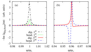
Figure 6: Skewness $-\operatorname{Im}\langle q_{\mathit{dip}}\rangle$ and bending $-\operatorname{Im}\langle q_{\mathit{bend}}\rangle$ of the cloud during the sloshing motion excited by $\hat{V}=\alpha x$ at $T/T_{F}=0.4$. In order to have comparable orders of magnitude, we multiplied the bending strengths by a factor $(\omega_{z}/\omega_{x})^{2}$. (a) In a harmonic trap, the unphysical skewness and bending of the first-order approximation (dash-dotted and dotted lines) are strongly suppressed when the third order moments are included (solid and dashed lines). Since in a harmonic trap there is no damping, we replaced $\omega$ by $\omega+i\,0.001\omega_{\perp}$ to generate this plot. (b) Skewness and bending during the sloshing motion in the anharmonic trap within the third-order approximation.

The existence of these distortions is in contradiction to the Kohn theorem and an unphysical consequence of the crude ansatz. At third order, owing to the additional degrees of freedom of the ansatz (28), the unphysical change of the cloud shape in the harmonic potential is strongly suppressed, as shown by the solid and dashed lines in Fig. 6(a).

While unphysical in a harmonic trap, a change of the cloud shape during the sloshing motion is expected in an anharmonic trap. From the preceding discussion it is clear that at least the third-order ansatz is required to get a meaningful description of this effect. In Fig. 6(b), third-order results for the expectation values of $q_{\mathit{dip}}$ and $q_{\mathit{bend}}$ during the sloshing motion are displayed. We note that, compared to the third-order results for a harmonic trap, both responses are now significantly increased, so that the peaks correspond to a real physical effect. Moreover, the observed shapes are typical of what one can obtain in a schematic model by coupling two damped modes (dipole and bending) to an undamped one (sloshing). Finally one can also see that the peaks are centered around the sloshing frequency, which is lower than in the harmonic case.

VI Collective modes related to cubic phase-space moments

In the previous section we have discussed coupling of the sloshing mode to other collective modes due to the trap anharmonicity. In particular, the ansatz (28) contains the necessary terms to describe the transverse compressional dipole and bending modes corresponding to the operators (31) and (33). In this section, we will study these modes in more detail. However, one should keep in mind that, since the excitation operators are already third-order ones, the ansatz (28) can only give the leading-order result for these modes.

Let us start with the radial dipole oscillation excited by the operator (31). In an ideal Fermi gas in an harmonic trap, this operator would excite two modes with frequencies $\omega/\omega_{\perp}=1$ and $3$.

In Fig. 7,

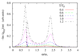
Figure 7: Strength function $-\operatorname{Im}\langle q_{\mathit{dip}}\rangle(\omega)$ for the radial dipole mode (excitation $\hat{V}=\alpha q_{\mathit{dip}}$) in the anharmonic trap for various temperatures. The parameters are the same as in Fig. 3.

the corresponding response function is shown for various temperatures. We see that in the collisionless regime, i.e., at high temperature, both modes exist but their frequencies are significantly lowered by the anharmonicity of the trap. Even at $T/T_{F}=1.2$ both modes are still very strongly damped (damping rate $\sim 0.3\omega_{\perp}$). At lower temperature, the damping gets so strong that both modes disappear completely: the hydrodynamic regime is not reached at any temperature. By artificially increasing the collision cross section to reach the hydrodynamic regime at $T/T_{F}=0.4$, we found that there would be a mode at $\sim 2\omega_{\perp}$ ($\sim 2.4\omega_{\perp}$ in the case of a harmonic trap), but in order to reach this regime in an experiment one would have to use a trap with a much lower radial frequency (i.e., a more spherical or even pancake-shaped trap). At the frequency of the sloshing mode, the response exhibits a characteristic dip due to the coupling between the dipole mode and the almost undamped sloshing mode (the sloshing is damped mainly because of this coupling).

In order to get a better understanding of the character of the two modes in the collisionless regime, we display their velocity fields in Fig. 8.

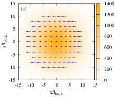
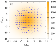
Figure 8: Velocity fields in the $x$-$y$ plane, averaged over $z$, corresponding to the dipole modes at $\omega\approx 0.8\omega_{\perp}$ (a) and $\omega\approx 2.3\omega_{\perp}$ (b) at $T=T_{F}$ (collisionless regime). The background color indicates the density per spin state integrated over $z$ in units of $l_{\mathit{ho},\perp}^{-2}$, with $l_{\mathit{ho},\perp}=1/\sqrt{m\omega_{\perp}}$.

Although both modes are excited by the same operator, their velocity fields are quite different. The velocity field of the low-lying mode ($\omega\approx 0.8\omega_{\perp}$ at $T=T_{F}$), cf. Fig. 8(a), confirms that this mode comprises both center-of-mass and skewness oscillations. The velocity field of the high-lying mode ($\omega\approx 2.3\omega_{\perp}$ at $T=T_{F}$), shown in Fig. 8(b), resembles that of the dipole compression modes in atomic nuclei, shown e.g., in Fig. 6 of LABEL:Serr.

Although in an axially symmetric trap the octupole mode does not couple to the sloshing mode, let us for the sake of completeness briefly discuss this mode. Like the dipole operator (31), the octupole operator (32) would excite two modes at $\omega/\omega_{\perp}=1$ and $3$ if the gas was collisionless and in a harmonic trap. The octupole response function for the realistic case is displayed in Fig. 9(a).

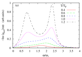
Figure 9: (a) Strength function $-\operatorname{Im}\langle q_{\mathit{oct}}\rangle(\omega)$ for the radial octupole mode (excitation $\hat{V}=\alpha q_{\mathit{oct}}$) in the anharmonic trap for various temperatures. The parameters are the same as in Fig. 3. (b) Velocity field corresponding to the high-lying mode at $T=T_{F}$ (see caption of Fig. 8 for details).

As in the dipole response, both modes are considerably shifted downwards because of the trap anharmonicity. The damping is even stronger than in the case of the dipole modes. Both octupole modes have a similar velocity field, as an example Fig. 9(b) shows that of the higher-lying mode. In a nuclear physics context it was found that their difference lies mainly in the non-diagonal pressure tensor (quadrupole moments in momentum space) KohlSchuck . At $T/T_{F}=0.4$, there is only a very broad peak around the hydrodynamic frequency $\omega/\omega_{\perp}=\sqrt{3}$ predicted in LABEL:GriffinWu1997 for a harmonic trap. However the strong damping shows that one is still far from the hydrodynamic regime. By increasing again artificially the cross-section, the hydrodynamic frequency is found to be lowered to $\simeq 1.58\omega_{\perp}$ due to anharmonicity.

Finally, in Fig. 10

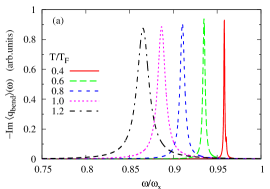
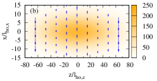
Figure 10: (a) Strength function $-\operatorname{Im}\langle q_{\mathit{bend}}\rangle(\omega)$ for the bending mode (excitation $\hat{V}=\alpha q_{\mathit{bend}}$) in the anharmonic trap for various temperatures. The parameters are the same as in Fig. 3. (b) Velocity field in the $x$-$z$ plane, averaged over $y$, corresponding to the bending mode at $T=T_{F}$. The background color indicates the density integrated over $y$ in units of $1/(l_{\mathit{ho},x}l_{\mathit{ho},z})$ with $l_{\mathit{ho},i}=1/\sqrt{m\omega_{i}}$.

we display the strength function and the velocity field of the bending mode. In a non-interacting gas in a harmonic trap, there would be three modes at $\omega=\omega_{x}$ and $\omega=\omega_{x}\pm 2\omega_{z}$. In the realistic case, these peaks cannot be resolved and one sees a damped oscillation with a frequency close to $\omega_{x}$. In fact, the behavior of its frequency and damping rate is qualitatively similar to that of the sloshing mode, but the temperature dependence of the frequency is stronger. Above $0.5T_{F}$, the damping is weaker than that of the sloshing mode, but this is probably an artefact of our approximation: We expect that the bending mode will receive an additional damping (analogous to that of the sloshing mode) from its coupling to a radial dipole mode modulated in $z$ [operator $(z^{2}-\langle z^{2}\rangle_{\mathit{eq}})q_{\mathit{dip}}$], which is not included in the third-order ansatz. Except at the lowest temperature, the mixing between sloshing and bending mode is weaker than that between sloshing and dipole mode, and the bending response does not show the characteristic dip that was found in the dipole response. The velocity field, shown in Fig. 10(b) confirms that this mode corresponds to a bending of the elongated cloud in the $x$-$z$ plane.

VII Conclusions

In this paper, we studied the frequency shift and damping of the sloshing mode of a normal-fluid Fermi gas in a realistic anharmonic trap potential. We used the moments method in order to find approximate solutions of the Boltzmann equation with mean field and in-medium cross-section. Already at first order, the moments method predicts a downwards shift of the frequency of the sloshing mode. However, the first order ansatz is insufficient to describe the coupling between the center-of-mass and the internal degrees of freedom of the gas, which is responsible for the damping of the sloshing mode in an anharmonic trap. We therefore extended the ansatz to include also third-order phase-space moments. The third-order ansatz contains not only the sloshing mode, but also more complicated radial dipole and bending modes. The important mechanism for the damping of the sloshing mode is its coupling to these modes (especially to the dipole mode) due to the trap anharmonicity. In addition, the third-order ansatz allowed us to discuss the radial octupole mode.

The comparison with the available experimental data for the sloshing mode shows that the essential features of the frequency shift can be reproduced. Quantitatively, the calculated ratios $\omega_{\mathit{slosh}}/\omega_{x}$ are somewhat lower than those given in LABEL:Riedl2008. Since both the mean field and the third-order moments give only small corrections to the frequency shift predicted by the first-order moments method, further improvements of the theory will probably give even smaller corrections. An effect which has not been considered in our linear-response study is the dependence of the sloshing frequency on the amplitude of the mode. However, this effect goes into the wrong direction, since the restoring force gets weaker with increasing amplitude (see Fig. 1) and therefore the frequency of the sloshing mode will be further reduced (cf. also WuZhang2012_3d ). As discussed in Sec. V.1, a possible explanation of the discrepancy is that the experimental trap frequency $\omega_{x}$ may have been slightly underestimated in the analysis of LABEL:Riedl2008. Actually, our results could be used to determine the true value of $\omega_{x}$.

The agreement between the calculated and measured damping rates of the sloshing mode is satisfactory and makes us confident that our approach contains the essential physics to describe the coupling between the sloshing and internal degrees of freedom. This may also help to better understand other effects where the dissipation of center-of-mass kinetic energy plays a role, such as the heating of the cloud due to laser-beam-pointing noise discussed in LABEL:SavardOHara97.

In addition to the sloshing mode, we studied the radial dipole and octupole modes and the bending mode in the $x$-$z$ plane. However, one should keep in mind that for these modes the third-order ansatz contains only the leading order, and higher-order corrections can be important. We found that, with the present trap parameters, the dipole and octupole modes do not behave hydrodynamically at any temperature. The frequencies of the dipole, octupole, and bending modes are more strongly affected by the anharmonicity than the frequency of the sloshing mode. For the dipole and octupole modes, this can be intuitively understood, since these higher-order modes are more sensitive to what happens at larger $r_{\perp}$, where the atoms feel the anharmonicity of the trap. The same argument should also apply to the radial quadrupole and scissors modes not studied in the present paper. One should therefore be careful when comparing theoretical results obtained for a harmonic trap with experimental ones (as done in Riedl2008 ; Chiacchiera2009 ; Chiacchiera2011 ), since the anharmonicity effects cannot be completely absorbed in a renormalized radial trap frequency.

As a final remark we note that a similar third-order ansatz as the one used here [Eq. (28) with $(x,p_{x})\leftrightarrow(z,p_{z})$] can be used to describe one of the higher-order axial modes studied recently by the Innsbruck group Sanchez_Thesis (the $k=2$ mode in the notation of Sanchez_Thesis , corresponding to a motion as shown in Fig. 4(b) but in $z$ instead of $x$ direction). Having more nodes than the usually considered collective modes, these kinds of modes are very interesting since they are closer to sound waves in uniform systems.

References

- (1) J. Kinast, S.L. Hemmer, M.E. Gehm, A. Turlapov, and J.E. Thomas, Phys. Rev. Lett. 92, 150402 (2004).
- (2) M. Bartenstein, A. Altmeyer, S. Riedl, S. Jochim, C. Chin, J. Hecker Denschlag, and R. Grimm, Phys. Rev. Lett. 92, 203201 (2004); A. Altmeyer, S. Riedl, C. Kohstall, M.J. Wright, J. Hecker Denschlag, and R. Grimm, e-print cond-mat/0611285 (2006).
- (3) J. Kinast, A. Turlapov, and J.E. Thomas, Phys. Rev. A 70 051401(R) (2004); J. Kinast, A. Turlapov, and J.E. Thomas, Phys. Rev. A 71, 029901(E) (2005).
- (4) A. Altmeyer, S. Riedl, C. Kohstall, M.J. Wright, R. Geursen, M. Bartenstein, C. Chin, J. Hecker Denschlag, and R. Grimm, Phys. Rev. Lett. 98, 040401 (2007).
- (5) A. Altmeyer, S. Riedl, M.J. Wright, C. Kohstall, J. Hecker Denschlag, and R. Grimm, Phys. Rev. A 76, 033610 (2007).
- (6) M.J. Wright, S. Riedl, A. Altmeyer, C. Kohstall, E.R. Sánchez Guajardo, J. Hecker Denschlag, and R. Grimm Phys. Rev. Lett. 99, 150403 (2007).
- (7) S. Riedl, E. R. Sánchez Guajardo, C. Kohstall, A. Altmeyer, M. J. Wright, J. Hecker Denschlag, and R. Grimm, G. M. Bruun and H. Smith, Phys. Rev. A 78, 053609 (2008).
- (8) W. Kohn, Phys. Rev. 123, 1242 (1961).
- (9) L. Brey, N.F. Johnson, and B.I. Halperin, Phys. Rev. B 40, 10647 (1989).
- (10) J.F. Dobson, Phys. Rev. Lett. 73, 2244 (1994).
- (11) R. Grimm, M. Weidemüller, and Y.B. Ovchinnikov, Adv. At. Mol. Opt. Phys. 42, 95 (2000).
- (12) L. Wu and Y. Zhang, Phys. Rev. A 85, 045601 (2012).
- (13) L. Sidorenkov and R. Grimm, unpublished; the present damping data have been obtained by reanalyzing the raw data of LABEL:Riedl2008.
- (14) L. Wu and Y. Zhang, Europhys. Lett. 97, 16003 (2012).
- (15) S. Chiacchiera, T. Lepers, D. Davesne, and M. Urban, Phys. Rev. A 79, 033613 (2009).
- (16) G.M. Bruun and H. Smith, Phys. Rev. A 75, 043612 (2007).
- (17) T. Lepers, D. Davesne, S. Chiacchiera, and M. Urban, Phys. Rev. A 82, 023609 (2010).
- (18) S. Chiacchiera, T. Lepers, D. Davesne, and M. Urban, Phys. Rev. A 84, 043634 (2011).
- (19) E.M. Lifshitz and L.P. Pitaevskii, Physical Kinetics, Landau-Lifshitz Course of Theoretical Physics, vol. 10 (Pergamon, Oxford, 1980).
- (20) J.P. da Providência, Nucl. Phys. A 489, 111 (1988).
- (21) A. Altmeyer, PhD Thesis (Innsbruck, 2007).
- (22) J. Kinast, A. Turlapov, J.E. Thomas, Q. Chen, J. Stajic, and K. Levin, Science 307, 1296 (2005).
- (23) Q. Chen, J. Stajic, and K. Levin, Phys. Rev. Lett. 95, 260405 (2005).
- (24) P. Massignan, G.M. Bruun, and H. Smith, Phys. Rev. A 71, 033607 (2005).
- (25) F.E. Serr, T.S. Dumitrescu, T. Suzuki, and C.H. Dasso, Nucl. Phys. A 404, 359 (1983).
- (26) H. Kohl, P. Schuck, and S. Stringari, Nucl. Phys. A 459, 265 (1986).
- (27) A. Griffin, W.-C. Wu, and S. Stringari, Phys. Rev. Lett. 78, 1838 (1997).
- (28) T.A. Savard, K.M. O’Hara, and J.E. Thomas, Phys. Rev. A 56, R1095 (1997).
- (29) E.R. Sánchez Guajardo, PhD Thesis (Innsbruck, 2011).