Nonlocal appearance of a macroscopic angular momentum

Abstract

We discuss a type of measurement in which a macroscopically large angular momentum (spin) is “created” nonlocally by the measurement of just a few atoms from a double Fock state. This procedure apparently leads to a blatant nonconservation of a macroscopic variable - the local angular momentum. We argue that while this gedankenexperiment provides a striking illustration of several counter-intuitive features of quantum mechanics, it does not imply a non-local violation of the conservation of angular momentum.

1 Motivation

Laloë laloe has recently pointed out a beautiful paradox in quantum physics. Suppose we have two Bose-Einstein condensates (BEC) polarized in opposite directions along the $z$-direction ketterle and we perform a measurement of the spin (angular momentum) along a transversal direction by absorbing particles emerging from one cloud or the other. Then it can be shown that a macroscopic angular momentum along a random transversal direction appears after the detection of only a few particles theory . Moreover, owing to the fact that the clouds can be imagined as having a very large spatial extension, apparently a large macroscopic angular momentum can be made to appear almost instantaneously at a distance. The effect, as in the Hanbury-Brown Twiss experiment, may be attributed to the lack of which-path information about the particles (we cannot know from which cloud they emerged). In this paper we show that this situation is by no means singular in quantum physics. The paradox originates from our tendency to attribute reality to the eigenvalue/eigenvector of an observable whenever we are in a position to predict with certainty the result of measuring it. The paper is organized as follows. In Section 2 we give a general discussion of conservation laws in quantum mechanics, with emphasis on the role of measurement. In Section 3 we give a brief review of the gedankenexperiment of Laloë. The resolution of the non-conservation paradox is presented in Section 4. Finally, in Section 5 we discuss the implications of the above for the issue of “reality” in quantum physics.

2 Measurement and conservation laws in quantum mechanics

In this section we attempt to clarify what is meant by conservation laws in quantum mechanics, and in particular how we are to interpret these laws as measurement enters the picture.

Both in quantum and classical mechanics, conserved quantities are associated with dynamical symmetries. In classical mechanics, a dynamical variable $A$ of a system ${\cal S}$ always has some precise real-numbered value $a$, and $A$ is conserved in any process involving ${\cal S}$ just as long as the value of $A$ continues to equal $a$. Suppose that $A$ has no explicit time-dependence and that ${\cal S}$ is subject to a conservative process governed by a Hamiltonian $H$ with no explicit time-dependence. Then $A$ is a conserved quantity of ${\cal S}$ if and only if $\left\{A,H\right\}=0$, where $\left\{\cdot,\cdot\right\}$ is the Poisson bracket.

In quantum mechanics, a dynamical variable $A$ of a system ${\cal S}$ is not assumed always to have some precise real-numbered value. Nevertheless, if $A$ is represented by a self-adjoint operator $\hat{A}$ with no explicit time-dependence and ${\cal S}$ is subject to a conservative process governed by a Hamiltonian $\hat{H}$ with no explicit time-dependence, then $A$ is said to be conserved if and only if it commutes with the Hamiltonian, $\left[\hat{A},\hat{H}\right]=0$. In the Schrödinger picture ${\cal S}$’s pure quantum state satisfies $\left|\psi(t)\right\rangle=\hat{U}(t)\left|\psi(0)\right\rangle$, where $\hat{U}(t)=\exp\left[-i\hat{H}t/\hbar\right]$. Then for the expectation value we have

$$\left\langle A\right\rangle_{t} \equiv \left\langle\psi(t)\left|\hat{A}\right|\psi(t)\right\rangle=\left\langle\psi(0)\hat{U}^{{\dagger}}(t)\left|\hat{A}\right|\hat{U}(t)\psi(0)\right\rangle$$ (1)

$$= \left\langle\psi(0)\left|\hat{A}\right|\psi(0)\right\rangle=\left\langle A\right\rangle_{0},$$ (2)

provided that $\left[\hat{A},\hat{H}\right]=0$. The same result follows immediately in the Heisenberg picture, where we can write $\hat{A}(t)\equiv\hat{U}^{{\dagger}}(t)\hat{A}\hat{U}(t)=\hat{A}(0)$. Similarly, all higher moments of $A$ are conserved while the state of $\cal{S}$ evolves unitarily according to $\hat{U}(t)$. If one now uses the spectral theorem to expand $\hat{A}$ in eigenvalues,

$$\hat{A}=\sum_{j}a_{j}|a\rangle_{jj}\langle a|,$$ (3)

one notices immediately that the probability distributions corresponding to any measurement result $a_{j}$ are conserved,

$$P_{j,|\psi\rangle}(t)=|_{j}\langle a|\psi(t)\rangle|^{2}=P_{j,|\psi\rangle}(0),$$ (4)

owing to the fact that the $|a\rangle_{j}$’s are also eigenvectors of the Hamiltonian $\hat{H}$. This provides another way to derive Eq. (1-2), namely $\left\langle A\right\rangle_{t}=\sum_{j}a_{j}P_{j}(t)=\sum_{j}a_{j}P_{j}(0)=\left\langle A\right\rangle_{0}$.

The definitions above only allow us to predict that the probability distribution of a conserved observable will not change after a unitary (Hamiltonian) evolution. They do not say anything about nonunitary processes, in particular about what we are allowed to say when a single measurement of a conserved quantity is performed. Since the work of Dirac and Von Neumann it has been common to regard measurement in quantum mechanics as a nonunitary process that projects a system’s pure quantum state onto an eigenstate $\left|a\right\rangle$ with eigenvalue $a$ equal to the result of the measurement. These processes are called projective measurements. Let us consider in more detail the following situation. Suppose that at $t=0$ we measure $A$ and we find the value $a_{k}$. Then at $t=0$ we can assign the state $|a\rangle_{k}$. We let the system evolve with the evolution operator $\hat{U}(t)=\exp[-i\hat{H}t/\hbar]$ into $\hat{U}(t)|a\rangle_{k}$. Then, at a time $t$, the probability of obtaining the result $a_{j}$ is

$$P_{j,k}(t)=|_{j}\langle a|\hat{U}(t)|a\rangle_{k}|^{2}$$ (5)

This probability is $P_{j,k}(t)=\delta_{jk}$ only if $\left[\hat{A},\hat{H}\right]=0$. This means that only in this case will we find (with certainty) the same value for the variable when we measure it again at the time $t$. This makes us think that $A$ has value $a_{k}$ in state $\hat{U}(t)|a\rangle_{k}$: That the variable is conserved not only in the sense that if we measure it we certainly find this same value, but that the value in some sense exists there between the measurements.

We can make this thought more precise by introducing the following interpretative principle:

Descriptive Completeness:

A dynamical variable $A$ of a system ${\cal S}$ has precise real-numbered value $a_{k}$ if and only if the pure quantum state of $A$ is an eigenstate $\left|a\right\rangle_{k}$ with eigenvalue $a_{k}$.

The statement above makes clear that there exists a distinction between the state of a system being an eigenstate of an operator (observable) and that observable actually assuming the corresponding eigenvalue. The Descriptive Completeness principle associates the two: it is a rather minimalistic statement of completeness of quantum theory, by proposing a one-to-one correspondence between only certain mathematical entities that appear in the theory and ontological entities. As we will show here, this interpretative principle, although it looks innocuous and natural, is at the core of the paradoxes we discuss. Thus quantum mechanics is not a descriptively complete theory, in the sense defined above.

Let us now examine some of the consequences of this rule, when used in conjunction with the quantum-mechanical unitary and nonunitary processes.

Unitary evolution: If this descriptive completeness rule is a valid way to interpret unitary evolution in quantum mechanics, the immediate consequence when analyzing conserved variables can be formulated as follows: If $A$ has value $a$ at $t_{1}$ on ${\cal S}$ and is conserved throughout the interval between $t_{1}$and $t_{2}$, then $A$ has value $a$ at $t_{2}$; while if $A$ has no value $a$ at $t_{1}$ and is conserved through the interval between $t_{1}$ and $t_{2}$, then $A$ has no value $a$ at $t_{2}$ - unitary evolution neither creates nor alters the value of a conserved variable.

Nonunitary processes: For nonunitary processes, a conservation law for dynamical variables can be formulated simply as: a dynamical variable $A$ is conserved in a projective measurement process on $\cal{S}$ if and only if, when applied to an initial eigenstate of $\hat{A}$ with eigenvalue $a$, the process results in a final eigenstate of $\cal{S}$ also with eigenvalue $a$. If this is used in conjunction with the Descriptive Completeness rule, we end up with the statement that if $A$ has value $a$ at $t_{1}$ on ${\cal S}$ and is conserved in a projective measurement from $t_{1}$to $t_{2}$, then $A$ has value $a$ at $t_{2}$. But, unlike for unitary evolution, if $A$ has no value $a$ at $t_{1}$ and is conserved in a projective measurement between $t_{1}$ and $t_{2}$, then $A$ does have some value $a$ at $t_{2}$: in this case, a dynamical variable acquires a value on projective measurement even if that variable is conserved during the process. A dynamical variable then takes on a precise real-numbered value as a result of a projective measurement in which that variable is conserved.

Note that nowhere here we have said anything about where in space the measurement happens. The claim of existence of a value is made for the entire system under discussion, irrespective of how large its spatial extension is and of the fact that the measurement process itself may be localized to only a small part of the system. The consequence of this is nonlocality: apparently, if the Descriptive Completeness rule were to hold, a projective measurement on a subsystem can produce instantaneously a value for a variable of another subsystem, no matter how far away. Clearly, this would violate conservation laws locally.

Laloë’s gedankenexperiment provides a dramatic illustration of three peculiar consequences of the implicit use of Descriptive Completeness for the understanding of measurement and conservation in a particular setup: A distant measurement on a double condensate may prompt the nonlocal appearance of some definite value of a conserved dynamical variable on a system, this value may be uniquely determined by the post-measurement state of that system, and (most striking) this value may be macroscopic, even though a distant microscopic measurement prompted its nonlocal appearance. Aspects of the situation described by Laloë are far from being unusual in the realm of quantum mechanics. The first two consequences should be familiar from earlier work in the foundations of quantum physics related to the Einstein-Podolsky-Rosen (EPR) paradox, to Bell states, and to Greenberger-Horne-Zeilinger (GHZ) states EPR ; Bohm ; GHZ . However, the third consequence, the apparent nonlocal emergence of a macroscopic value as a consequence of a distant microscopic measurement process, is new.

3 Laloë’s gedankenexperiment

Let us now briefly review the situation analyzed in laloe . Consider BEC gases with atoms in two internal states, see Fig. (1). Because any two-level system is mathematically equivalent to a spin-1/2, we can regard the two states as being the states ”up” $|\uparrow\rangle$ and ”down” $|\downarrow\rangle$ of a spin along the $z$-direction. We will denote from now on by $|\pm\rangle_{\vec{n}}$ the two eigenvectors of the spin-1/2 along a direction $\vec{n}$, in other words $(\vec{n}\cdot\vec{\hat{\sigma}})|\pm\rangle_{\vec{n}}=\pm|\pm\rangle_{\vec{n}}$. In particular, $|\uparrow\rangle=|+\rangle_{z}$ and $|\downarrow\rangle=|-\rangle_{z}$. Now we prepare independently two condensates, one in which all the particles are in the state $|\uparrow\rangle$, and the other one in which they are in the state $|\downarrow\rangle$. For simplicity we take the number of particles in each state as equal $N_{\uparrow}=N_{\downarrow}=N/2$, where $N$ is the total number of particles. The system can then be described by a double Fock state

$$|\Psi\rangle_{\mathrm{initial}} = |N_{\uparrow}\rangle|N_{\downarrow}\rangle$$ (6)

$$= \frac{1}{\sqrt{N_{\uparrow}!}\sqrt{N_{\downarrow}!}}\left[\hat{a}_{\uparrow}^{{\dagger}}\right]^{N_{\uparrow}}\left[\hat{a}_{\downarrow}^{{\dagger}}\right]^{N_{\downarrow}}|\mathrm{vac}\rangle,$$ (7)

where $\hat{a}_{\downarrow}$, $\hat{a}_{\downarrow}^{{\dagger}}$ and $\hat{a}_{\uparrow}$, $\hat{a}_{\uparrow}^{{\dagger}}$ are the respective bosonic annihilation and creation operators for spin-down and spin-up atoms.

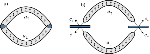
Figure 1: (a) Two condensates prepared in a double Fock spin state, and overlapping in two regions of space. Photon absorption measurement in one region results in the establishment of a macroscopic spin in a direction perpendicular to the initial polarization. (b) Equivalent measuring system using beam splitters.

Now the atoms are detected such that which-path information cannot be obtained (i.e. it is not possible to identify from which cloud, $\uparrow$ or $\downarrow$, the particles came). In the real interference experiment ketterle , this was achieved by absorption of photons in a certain region in space where the condensates overlap (Fig. 1a). The effect may be easier to understand if one thinks in terms of a two-channel beam-splitter measurement (Fig. 1b). In this case, the measurement of a single particle can be described by the action of the operators

$$\hat{c}_{\pm}=\frac{1}{\sqrt{2}}(\hat{a}_{\uparrow}\pm\hat{a}_{\downarrow}).$$ (8)

This is in fact a measurement of the spin along the $x$ direction of particles coming from the two clouds. The signs $\pm$ correspond to finding a particle with spin-component $\pm$ along the $x$ axis. To convince ourselves that this is the case, we recall that in second quantization the number of particles operator is

$$\hat{n}=\hat{a}_{\uparrow}^{{\dagger}}\hat{a}_{\uparrow}+\hat{a}_{\downarrow}^{{\dagger}}\hat{a}_{\downarrow},$$ (9)

and the spin along the $x$ direction is

$$\hat{\sigma}_{x}=\hat{a}_{\uparrow}^{{\dagger}}\hat{a}_{\downarrow}+\hat{a}_{\downarrow}^{{\dagger}}\hat{a}_{\uparrow}.$$ (10)

We can immediately prove the identity

$$\frac{1}{2}(\hat{n}\pm\hat{\sigma}_{x})=\hat{c}_{\pm}^{{\dagger}}\hat{c}_{\pm}.$$ (11)

Since in our experiment the particles are detected one at a time, we recognize on the left-hand side of Eq. (11) the first-quantized projection operator $\frac{1}{2}(I\pm\hat{\sigma}_{x})$ for the measurement of spin in the $x$ direction with results $\pm$. The left-hand side is the number operator for detection in the $\pm$ channels in Fig. (1b). Thus, the measurement along the $x$ direction is realized by counting the detections in each of these channels. The surprising result is that the repeated application of $\hat{c}_{\pm}$ (or $\hat{c}_{\pm}^{{\dagger}}\hat{c}_{\pm}$ if one wants to conserve the number of particles) results in the appearance of phase coherence between the $\uparrow$ and $\downarrow$ components. The number of detection events $N_{d}$ after which this phase is established does not have to be macroscopic for the system to acquire phase-coherence; typically after only a few tens of detections the system approaches to a good approximation the state

$$|\Psi\rangle_{\mathrm{after}}=\frac{1}{\sqrt{(N-N_{d})!}}\hat{c}_{\varphi}^{{\dagger}(N-N_{d})}|\mathrm{vac}\rangle.$$ (12)

Here

$$\hat{c}_{\varphi}=\frac{1}{\sqrt{2}}(\hat{a}_{\uparrow}+e^{i\varphi}\hat{a}_{\downarrow})$$ (13)

is the annihilation operator along a direction given by the unit vector $\vec{n}_{\varphi}$ in the $xOy$ plane which makes some angle $\varphi$ with $Ox$. The state Eq. (12) is an eigenvalue of the total spin component $(\hbar/2)\sum_{i=1,N-N_{d}}\vec{\hat{\sigma}}\cdot\vec{n}_{\varphi}$ along this direction, with a macroscopic value $(\hbar/2)(N-N_{d})$. Indeed, $(\hbar/2)\hat{c}_{\varphi}^{{\dagger}}\hat{c}_{\varphi}|\Psi\rangle_{\mathrm{after}}=(\hbar/2)(N-N_{d})|\Psi\rangle_{\mathrm{after}}$. The phase $\varphi$ emerging after this sequence of measurements is random, in the sense that repeating the experiment produces in general a different value for $\varphi$. Note that the initial state Eq. (7) does not have a well-defined phase along any direction. Here we have a situation in which apparently a microscopic process (note that $N_{d}$ can be much smaller than $N$) led to the appearance of a macroscopic quantity.

Moreover, the two clouds may be imagined to overlap only in two widely separated regions, as in Fig. (1). In this case, the $N_{d}$ detections in one region prompts the almost instantaneous appearance at a distance of a macroscopic angular momentum in the other region.

4 Nonlocal creation of angular momentum?

Let us now discuss in more detail the mechanism by which this macroscopic angular momentum is apparently created nonlocally. We show that in the end this paradox is not conceptually different from the situation of standard EPR-type experiments.

As before, the measurement process is described only by the operator $\hat{c}_{\pm}$. Before the first detection the probabilities to obtain the results $\pm$ are equal, 1/2. Suppose now that the first particle is detected and the result is $+$. Then, after applying the operator $\hat{c}_{+}$ to $|N_{\uparrow}N_{\downarrow}\rangle$, we get the many-body wavefunction

$$\frac{1}{\sqrt{N}}\left[\sqrt{N_{\uparrow}}|N_{\uparrow}-1,N_{\downarrow}\rangle+\sqrt{N_{\downarrow}}|N_{\uparrow},N_{\downarrow}-1\rangle\right]$$ (14)

We now ask again what is the probability of getting the results $\pm$; these can be calculated by applying $c_{\pm}$ on the wavefunction Eq. (14) and taking the square modulus of each of the two results. In the limit of large number of particles, $N\gg 1$, we find that the probability of obtaining the result $+$ is now 3/4 while that of obtaining the result $-$ is 1/4. Thus the previous detection, with the result $+$, has modified the probabilities for the next detection, favoring a $+$ result. Now if a $+$ result is obtained again, the probability to find $+$ at the next detection is 5/6. In general, the probability to obtain $+$ after previous $k$ consecutive $+$ detections is $(2k+1)/2(k+1)$, which very quickly approaches 1. Thus after only a few consecutive $+$ detections, the wavefunction becomes very close to an eigenvector of the operator $c_{+}$.

Let us now do the same calculation in the situation where we know where the particles come from. For example, we either block one of the condensates, move it further, or controllably release particles from either one of them. Suppose that for the detection of the first particles we choose the condensate with $\uparrow$, and suppose, as before, that we get the result $+$. We again find the state of the system after this detection by applying $c_{+}$, but this time on $|N_{\uparrow}\rangle|\mathrm{vac}\rangle$. For the next detection, we can choose to use either $\uparrow$ atoms or $\downarrow$ atoms. In both cases, we obtain equal probabilities for the results $\pm$! In general, after $k_{\uparrow}$ atoms have been extracted from the cloud $\uparrow$ and $k_{\downarrow}$ from the cloud $\downarrow$, the overall state of the system remains a Fock state $|N_{\uparrow}-k_{\uparrow},N_{\downarrow}-k_{\downarrow}\rangle$.

Thus the essential ingredient for obtaining the phase is lack of which-path information about which cloud the detected particles have originated from. This is embedded in the definition of the operators $\hat{c}_{\pm}$ as superpositions between $\hat{a}_{\uparrow}$ and $\hat{a}_{\downarrow}$. It almost looks like our ignorance has created a macroscopic spin component in the $xOy$ plane! Of course, the two situations (availability or not of which-way information) correspond to physically different setups. But these setups are local, and, if we accept the Descriptive Completeness principle, it seems possible to determine, from a spatially separated location, whether a macroscopic element of reality pops up into existence or not.

Our resolution of the “paradox” appeals to two separate measurement setups. The first one is Alice’s, who measures transverse components of spin on a relatively small number of particles in a tiny region where the two clouds overlap: While in the second, Bob measures the total transverse spin-component of the overlapping clouds in a large, distant region along just the direction in which this is then almost certain to record a macroscopic result. If we treat Alice’s measurement as projective, then it puts the total condensate into a state which is very close to an eigenstate of spin-component along the direction Bob happens to measure, corresponding to a macroscopic eigenvalue. Now, when Bob measures this spin-component on the large cloud of condensate in his region, far from Alice, he is almost certain to get a macroscopic result. But this does not mean that Alice’s measurement produces a “real” macroscopic value of angular momentum in Bob’s region. Bob’s measurement does not simply reveal this macroscopic value of a pre-existing spin-component of or in the cloud produced by Alice’s projective measurement. Instead, the macroscopic spin-component in Bob’s region “emerges” during Bob’s measurement following an interaction with Bob’s measuring device. There is no reason to suspect that this local interaction involves any violation of the conservation of angular momentum. Certainly, nothing that happens near Alice creates a macroscopic angular momentum near Bob in violation of local conservation of angular momentum. Thus our conclusion is that Laloë’s gedanken-experiment involves no nonlocal failure of the conservation law of angular momentum, but rather that it reveals that Descriptive Completeness is not a valid principle in quantum physics.

To revisit the structure of the argument, we emphasize the following two key points:

1. in the natural way of extending the standard analysis of conservation of an observable to cover the case of projective measurement, a conserved observable with no prior definite value may acquire an eigenvalue on projective measurement,

2. but after a subsystem ${\cal S}_{1}$ of a composite system ${\cal S}_{1}\otimes{\cal S}_{2}$ is put into an eigenstate of an observable following a projective measurement on a distinct subsystem ${\cal S}_{2}$, one cannot immediately infer that the observable has the corresponding eigenvalue on ${\cal S}_{1}$: one can infer only that a measurement of that observable will certainly reveal that value. So an inference from a quantum state to a value of an observable is not always valid even when that state is an eigenstate of that observable.

5 Conclusions and further discussions: does angular momentum exist?

Franck Laloë laloe notices the apparent nonconservation of angular momentum for a double Fock state and concludes that (barring controversial interpretations such us Everett’s) we are almost inevitably forced to agree with the EPR conclusion that this state does not provide a complete description of the physical system (i.e. Descriptive Completeness fails).

If the wavefunction is not an element of reality (or a representation of one) but just a tool to predict the results of measurements, then there is no paradox. The macroscopic angular momentum simply appears in the very act of measuring a macroscopic angular momentum. Note that this is true whether or not the measured system’s pre-measurement quantum state is an eigenstate of that angular momentum (or other quantity) that is measured. In the Stern-Gerlach apparatus the angular momentum does not appear until the particles interact one by one with the detector after passing the magnets. In this example, the initial wavefunction is not an eigenstate of spin component ($\pm 1$) along $x$ but a superposition. On the other hand, in Laloë’s example the wavefunction after the distant microscopic measurements but before a local measurement of angular momentum is (very nearly) an eigenstate of angular momentum along a direction in the $xOy$ plane which makes some angle $\varphi$ with $Ox$. In this respect the situation described by Laloë mirrors the GHZ states: there, following (two) distant measurements we also have an eigenvalue of a local observable to which we cannot attribute physical reality prior to its measurement even when the state of the system is an eigenstate of that observable.

This of course leaves us with the question: When a system is prepared in an eigenstate of an observable, what “exists” out there? The only answer that standard quantum theory provides peresbohr is simply: This wavefunction refers to an ensemble of identically prepared systems, on which a device for measuring that observable will record the (same) corresponding eigenvalue for each system. This in no way implies that this value exists as an intrinsic property of each of the components of the ensemble, an implication that also fails on a less operationalist answer (favored by one of us healey ). On this latter, pragmatist approach, one is licensed to infer from a system’s being assigned an eigenstate of an observable to its having the corresponding eigenvalue only in so far as the joint state of system and environment has decohered with eigenstates of the observable corresponding to a “pointer basis”. In the situation described by Laloë the surprising thing is also that apparently a microscopic interaction (the measurement of a relatively small number of particles) has a macroscopic outcome: the appearance of a large angular momentum. The same paradox of a very small quantity flipping a macroscopic one appears in the analysis of the Josephson effect leggettsols .

Similarly in the case of the Bose-Einstein double condensate, after a small number of transversal measurements, we end up in a state which approximates an eigenstate of the angular momentum along a direction in the $xOy$ plane with a large eigenvalue. Again, we tend to imagine this state and the corresponding angular momentum existing. Just as in the Bloch sphere representation, where the eigenvectors of the spin can be mathematically identified with arrows pointing in some direction, we tend to believe that these arrows represent something real. But the arrows correspond to quantum state assignments, not assignments of values to observables in those states. Even for an assignment of an angular momentum eigenstate to a system, it is only at the end of a measurement that we can say that the system has an angular momentum component in the direction of the arrow equal to the corresponding eigenvalue. There is no angular momentum before it was measured.

One can object to all the above by saying; but isn’t it the case that the total spin of a ferromagnet is “real”? Isn’t it the case that the existence of a “real” angular momentum is established by experiments such as Einstein - de Haas? To this we can only answer: all experiments in physics end with a measurement. The lesson we learn from quantum physics is that it is real because it is has a measured value. It is not the case that something has a measured value because it is real. In many practical situations in physics we do not need to distinguish between the two: but sometimes we are forced to admit that they are different.

6 Acknowledgements

The research for this work was initially funded by the Templeton Research Fellows Program “Philosophers - Physicists Cooperation Project on the Nature of Quantum Reality” at the Austrian Academy of Science s Institute for Quantum Optics and Quantum Information, Vienna, which allowed the authors to spend the summer of 2009 at IQOQI Vienna. Special thanks go to our hosts in Vienna, Prof. A. Zeilinger and Prof. M. Aspelmeyer, who have made this visit possible, and additionally to the scientists in the institute for many enlightening discussions. Also, GSP acknowledges support from the Academy of Finland (Acad. Res. Fellowship 00857, and projects 129896, 118122, 135135, and 141559). The contribution by RH to this material is partially based upon work supported by the National Science Foundation under Grant No. SES-0848022.

References

- (1) F. Laloë: Bose-Einstein condensates and EPR quantum non-locality. In: T.M. Nieuwenhuizen et. al. (eds.) Beyond the Quantum, pp. 35-52. World Scientific, Singapore (2007); arXiv:0704.0386.
- (2) Andrews, M.R., et. al.: Observation of interference between two Bose condensates, Science 275, 637-641 (1997).
- (3) J. Javanainen and S. M. Yoo: Quantum phase of a Bose-Einstein condensate with an arbitrary number of atoms. Physical Review Letters 76, 161-4 (1996); Castin, Y. and Dalibard, J.: Relative phase of two Bose-Einstein condensates. Physical Review A 55, 4330-7 (1997); Laloë, F.: The hidden phase of Fock states; quantum non-local effects. The European Physics Journal D 33, 87-97 (2005); Mullin, W.J., Krotkov, R. and Laloë, F.: Evolution of additional (hidden) quantum variables in the interference of Bose-Einstein condensates. Physical Review A 74, 023610:1-11 (2006); Mullin, W.J., Krotkov, R. and Laloë, F.: The origin of the phase in the interference of Bose-Einstein condensates. American Journal of Physics 74, 880-87 (2006); Laloë, F. and Mullin, W.J.: Einstein-Podolsky-Rosen argument and Bell inequalities for Bose-Einstein spin condensates. Physical Review A 77, 022108:1- 17 (2008); Paraoanu, G.S.: Localization of the relative phase via measurements. Journal of Low Temperature Physics 153, 285-93 (2008).
- (4) A. Einstein, B. Podolsky, and N. Rosen: Can quantum-mechanical description of reality be considered complete? Phys. Rev. 47, 777-780 (1935).
- (5) D. Bohm: (1951) Quantum Theory. Prentice-Hall, New York.
- (6) D. M. Greenberger, M. A. Horne, and A. Zeilinger, (1989) in Bell’s Theorem, Quantum Theory, and Conceptions of the Universe, ed. M. Kafatos, 73-76. Kluwer, Dordrecht.
- (7) R. Healey: Quantum Theory: a Pragmatist Approach, forthcoming in the British Journal for the Philosophy of Science, arXiv:1008.3896.
- (8) Peres, A.: Quantum Theory: Concepts and Methods. Dordrecht: Kluwer Academic (1993).
- (9) Leggett, A.J. and Sols, F.: On the concept of spontaneously broken gauge symmetry in condensed matter physics. Foundations of Physics 21, 353-364 (1991).