Abstract: Two independent Poisson streams of jobs flow into a single-server service system having a limited common buffer that can hold at most one job. If a type-$i$ job ($i=1,2$) finds the server busy, it is blocked and routed to a separate type-$i$ retrial (orbit) queue that attempts to re-dispatch its jobs at its specific Poisson rate. This creates a system with three dependent queues. Such a queueing system serves as a model for two competing job streams in a carrier sensing multiple access system. We study the queueing system using multi-dimensional probability generating functions, and derive its necessary and sufficient stability conditions while solving a boundary value problem. Various performance measures are calculated and numerical results are presented.

Key-words: Retrial queues, Riemann-Hilbert boundary value problem, Carrier sensing multiple access system

Files d’attente avec réémissions des clients et un serveur unique

Résumé : Un serveur unique ’exponentiel’, sans file d’attente, est alimenté par deux flux poissonniens et indépendants de clients. Un client du flux $i$ ($i=1,2$) trouvant le serveur unique inoccupé est servi et quitte le système une fois servi; s’il trouve le serveur unique occupé alors il rejoint une file d’attente, appelée orbite $i$, de capacité illimitée et équipée d’un serveur ’exponentiel’. Un client quittant l’orbite $i$ est routé vers le serveur unique; si celui-ci est inoccupé alors il quitte le système une fois servi; s’il est occupé alors il est de nouveau routé vers l’orbite $i$ et le processus décrit ci-dessus se répète. Le tout créé ainsi un système composé de trois file d’attente fortement corrélées. Ce système de files d’attente sert à modeliser des protocoles de communication à contention. Nous établissons une équation satisfaite par la fonction génératrice jointe du nombre de clients dans les trois files d’attente, que nous résolvons par réduction à un problème aux limites de Riemann-Hilbert. Nous déterminons la condition de stabilité du système et concluons le rapport en présentant des résultats numériques pour les principales mesures de performance.

Mots-clés : Files d’attente réémissions des clients, Problème aux limites de Riemann-Hilbert, Protocoles de communication à contention

1 Introduction

Queues with blocking and with retrials have been studied extensively in the literature (see e.g. [1]-[7], [12]-[14], [16], [17], [25] and references therein). In this paper we investigate a single-server system with two independent exogenous Poisson streams flowing into a common buffer that can hold at most one job. If a type-$i$ job finds the server busy, it is routed to a separate retrial (orbit) queue from which jobs are re-transmitted at a Poisson rate. Such a queueing system serves as a model for two competing job streams in a carrier sensing multiple access system, where the jobs – after a failed attempt to network access – wait in an orbit queue [23, 24]. The two types of customers can be interpreted as customers with different priority requirements. An important feature of the retrial system under consideration is a constant retrial rate. The constant retrial rate helps to stabilize the multiple access system [8]. The retrial queueing systems with a constant retrial rate and a single type of jobs has been considered in [3]-[7], [13]-[14], [17]. We formulate this system as a three-dimensional Markovian queueing network, and derive its necessary and sufficient stability conditions. Recently these stability conditions have been shown by simulations to hold even in a more general system with generally distributed service times [7].

The structure of the paper is as follows: After the Introduction we present the model in Section 2. Balance equations and generating functions are derived in Section 3, while necessary stability conditions are obtained in Section 4. Using the technique developed by Fayolle and Iasnogoroski [18], in Section 5 we show that these generating functions are obtained, in closed-form, via the solution of a Riemann-Hilbert boundary value problem. This approach allows us to show that the necessary stability conditions found in Section 4 are also sufficient. Performance measures are calculated in Section 6, and numerical results are presented in Section 7. In particular, our numerical results demonstrate that the proposed multiple access system with two types of jobs and constant retrial rates provides incentives for the users to respect the contracts.

2 Model

Two independent Poisson streams of jobs, $S_{1}$ and $S_{2}$, flow into a single-server service system. The service system can hold at most one job. The arrival rate of stream $S_{i}$ is $\lambda_{i}$, $i=1,2$, with $\lambda:=\lambda_{1}+\lambda_{2}$. The required service time of each job is independent of its type and is exponentially distributed with mean $1/\mu$. If an arriving type-$i$ job finds the (main) server busy, it is routed to a dedicated retrial (orbit) queue that operates as an $\cdot/M/1/\infty$ queue. That is, blocked jobs of type $i$ form a type-$i$ single-server orbit queue that attempts to retransmit jobs (if any) to the main service system at a Poisson rate of $\mu_{i}$, $i=1,2$. Thus, the overall system is comprised of three queues as depicted in Figure 1.

Figure 1: Retrial system with two orbit queues.

3 Balance equations and generating functions

Consider the system in steady state. Let $L$ denote the number of jobs in the main queue. $L$ assumes the values of 0 or 1. Let $Q_{i}$ be the number of jobs in orbit-queue $i$, $i=1,2$. The transition-rate diagram of the system is depicted in Figure 2. The numbers 0 or 1 appearing next to each node indicate whether $L=0$ or $L=1$, respectively.

Define the set of stationary probabilities $\{P_{mn}(k)\}$ as follows:

$$P_{mn}(k)=P(Q_{1}=m,Q_{2}=n,L=k),\quad m,n=0,1,2,...\quad k=0,1.$$

Define the marginal probabilities

$$P_{m\bullet}(k)=\sum_{n=0}^{\infty}P_{mn}(k)=P(Q_{1}=m,L=k),\quad m=0,1,2,...\quad k=0,1,$$

and

$$P_{\bullet n}(k)=\sum_{m=0}^{\infty}P_{mn}(k)=P(Q_{2}=n,L=k),\quad n=0,1,2,...\quad k=0,1.$$

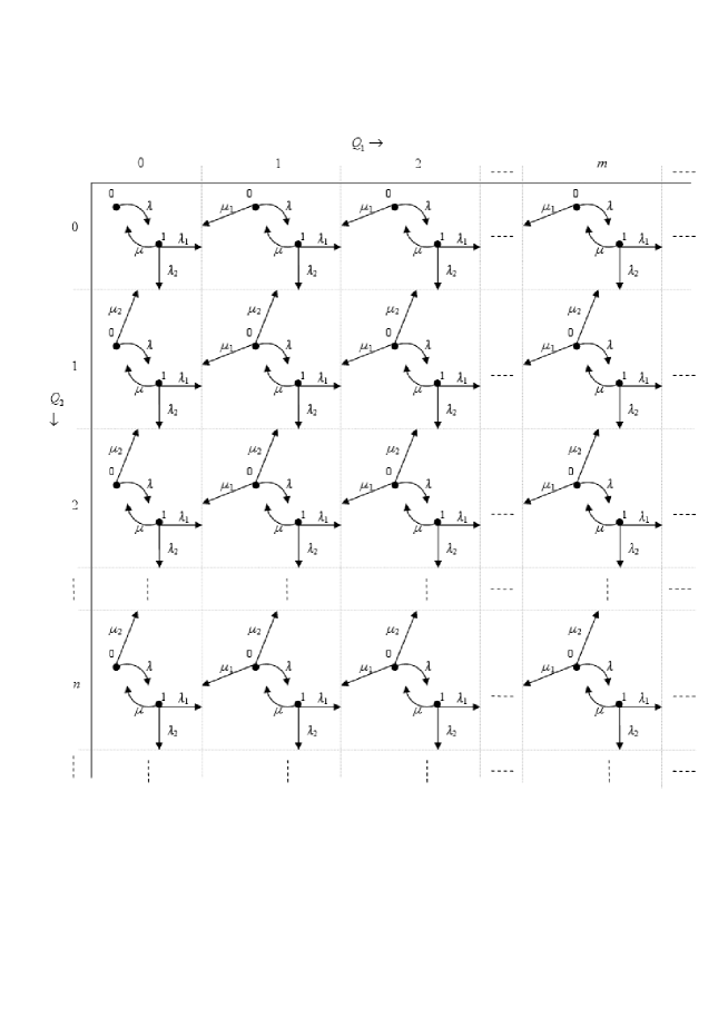
Figure 2: Transition-rate diagram.

Let us write the balance equations. If $Q_{2}=0$, we have

• for $Q_{1}=0$ and $k=0$,

  $$\lambda P_{00}(0)=\mu P_{00}(1),$$ (1)

• for $Q_{1}=m\geq 1$ and $k=0$,

  $$(\lambda+\mu_{1})P_{m0}(0)=\mu P_{m0}(1),$$ (2)

• for $Q_{1}=0$ and $k=1$,

  $$(\lambda+\mu)P_{00}(1)=\lambda P_{00}(0)+\mu_{1}P_{10}(0)+\mu_{2}P_{01}(0),$$ (3)

• for $Q_{1}=m\geq 1$ and $k=1$,

  $$(\lambda+\mu)P_{m0}(1)=\lambda P_{m0}(0)+\mu_{1}P_{m+1,0}(0)+\mu_{2}P_{m1}(0)+\lambda_{1}P_{m-1,0}(1).$$ (4)

If $Q_{2}=n$, $n\geq 1$, we have

• for $Q_{1}=0$ and $k=0$,

  $$(\lambda+\mu_{2})P_{0n}(0)=\mu P_{0n}(1),$$ (5)

• for $Q_{1}=m\geq 1$ and $k=0$,

  $$(\lambda+\mu_{1}+\mu_{2})P_{mn}(0)=\mu P_{mn}(1),$$ (6)

• for $Q_{1}=0$ and $k=1$,

  $$(\lambda+\mu)P_{0n}(1)=\lambda P_{0n}(0)+\mu_{1}P_{1n}(0)+\mu_{2}P_{o,n+1}(0)+\lambda_{2}P_{0,n-1}(1),$$ (7)

• for $Q_{1}=m\geq 1$ and $k=1$,

  $$(\lambda+\mu)P_{mn}(1)=\lambda P_{mn}(0)+\mu_{1}P_{m+1,n}(0)+\mu_{2}P_{m,n+1}(0)$$

  $$+\lambda_{1}P_{m-1,n}(1)+\lambda_{2}P_{m,n-1}(1).$$ (8)

Let us define the following Probability Generating Functions (PGFs):

$$G_{n}^{(k)}(x)=\sum_{m=0}^{\infty}P_{mn}(k)x^{m},\quad k=0,1,\quad n\geq 0.$$

Then, for $n=0$ and $k=0$, multiplying each equation from (1) and (2) by $x^{m}$, respectively, and summing over $m$ results in

$$\lambda\sum_{m=0}^{\infty}P_{m0}(0)x^{m}+\mu_{1}\sum_{m=1}^{\infty}P_{m0}(0)x^{m}=\mu\sum_{m=0}^{\infty}P_{m0}(1)x^{m},$$

or

$$(\lambda+\mu_{1})G_{0}^{(0)}(x)-\mu_{1}P_{00}(0)=\mu G_{0}^{(1)}(x).$$ (9)

Similarly, for $n=0$ and $k=1$, using equations (3) and (4) leads to

$$(\lambda+\mu)G_{0}^{(1)}=\lambda G_{0}^{(0)}+\mu_{1}\sum_{m=0}^{\infty}P_{m+1,0}(0)x^{m}+\mu_{2}G_{1}^{(0)}(x)+\lambda_{1}\sum_{m=1}^{\infty}P_{m-1,0}(1)x^{m}.$$

That is,

$$(\lambda+\mu)G_{0}^{(1)}(x)=\lambda G_{0}^{(0)}(x)+\frac{\mu_{1}}{x}(G_{0}^{(0)}(x)-P_{00}(0))+\mu_{2}G_{1}^{(0)}(x)+\lambda_{1}xG_{0}^{(1)}(x).$$

Multiplying by $x$ and arranging terms, we obtain

$$-(\lambda x+\mu_{1})G_{0}^{(0)}(x)+(\lambda_{1}(1-x)+\lambda_{2}+\mu)xG_{0}^{(1)}(x)-\mu_{2}xG_{1}^{(0)}(x)=-\mu_{1}P_{00}(0).$$ (10)

Using equations (5) and (6) for $n\geq 1$ and $k=0$ results in

$$(\lambda+\mu_{2})G_{n}^{(0)}(x)+\mu_{1}(G_{n}^{(0)}(x)-P_{0n}(0))=\mu G_{n}^{(1)}(x),$$

or

$$(\lambda+\mu_{1}+\mu_{2})G_{n}^{(0)}(x)-\mu G_{n}^{(1)}(x)=\mu_{1}P_{0n}(0).$$ (11)

Similarly, for $n\geq 1$ and $k=1$, equations (7) and (8) lead to

$$(\lambda+\mu)G_{n}^{(1)}(x)=\lambda G_{n}^{(0)}(x)+\frac{\mu_{1}}{x}(G_{n}^{(0)}(x)-P_{0n}(0))+\mu_{2}G_{n+1}^{(0)}(x)$$

$$+\lambda_{1}xG_{n}^{(1)}(x)+\lambda_{2}G_{n-1}^{(1)}(x),$$

or

$$-(\lambda x+\mu_{1})G_{n}^{(0)}(x)+(\lambda_{1}(1-x)+\lambda_{2}+\mu)xG_{n}^{(1)}(x)-\mu_{2}xG_{n+1}^{(0)}(x)$$

$$-\lambda_{2}xG_{n-1}^{(1)}(x)=-\mu_{1}P_{0n}(0).$$ (12)

Define now the two-dimensional PGFs

$$H^{(k)}(x,y)=\sum_{n=0}^{\infty}\sum_{m=0}^{\infty}P_{mn}(k)x^{m}y^{n}=\sum_{n=0}^{\infty}G_{n}^{(k)}(x)y^{n},\quad k=0,1.$$ (13)

Using equations (9) and (11), multiplying respectively by $y^{n}$ and summing over $n$, we obtain

$$(\lambda+\mu_{1})H^{(0)}(x,y)+\mu_{2}(H^{(0)}(x,y)-G_{0}^{(0)}(x))-\mu H^{(1)}(x,y)=\mu_{1}H^{(0)}(0,y).$$ (14)

Similarly, using equations (10) and (12), we obtain

$$-(\lambda x+\mu_{1})H^{(0)}(x,y)+(\lambda_{1}(1-x)+\lambda_{2}+\mu)xH^{(1)}(x,y)$$

$$-\frac{\mu_{2}x}{y}(H^{(0)}(x,y)-G_{0}^{(0)}(x))-\lambda_{2}xyH^{(1)}(x,y)=-\mu_{1}H^{(0)}(0,y).$$ (15)

Noting that $G_{0}^{(0)}(x)=H^{(0)}(x,0)$ and denoting $\alpha:=\lambda+\mu_{1}+\mu_{2}$, we can rewrite equations (14) and (15) as

$$\alpha H^{(0)}(x,y)-\mu H^{(1)}(x,y) = \mu_{2}H^{(0)}(x,0)+\mu_{1}H^{(0)}(0,y),$$ (16)

$$(\lambda xy+\mu_{1}y+\mu_{2}x)H^{(0)}(x,y) - (\lambda_{1}(1-x)+\lambda_{2}(1-y)+\mu)xyH^{(1)}(x,y)$$ (17)

$$= \mu_{2}xH^{(0)}(x,0)+\mu_{1}yH^{(0)}(0,y),$$

or, equivalently, in a matrix form

$${\bf C}(x,y){\bf H}(x,y)={\bf g}(x,y),$$ (18)

where

$${\bf C}(x,y)=\left[\begin{array}[]{cc}\alpha&-\mu\\ \lambda xy+\mu_{1}y+\mu_{2}x&-(\lambda_{1}(1-x)+\lambda_{2}(1-y)+\mu)xy\end{array}\right],$$

$${\bf H}(x,y)=\left[\begin{array}[]{c}H^{(0)}(x,y)\\ H^{(1)}(x,y)\end{array}\right],$$

$${\bf g}(x,y)=\left[\begin{array}[]{c}\mu_{2}H^{(0)}(x,0)+\mu_{1}H^{(0)}(0,y)\\ \mu_{2}xH^{(0)}(x,0)+\mu_{1}yH^{(0)}(0,y)\end{array}\right].$$

Now, if we calculate $H^{(0)}(x,0)$ and $H^{(0)}(0,y)$, the two-dimensional PGF ${\bf H}(x,y)$ is immediately obtained from equation (18).

4 Necessary stability conditions

Proposition 4.1

$$H^{(1)}(1,1)=P(L=1)=\frac{\lambda}{\mu}$$ (19)

and

$$H^{(0)}(0,1) = P(Q_{1}=0,L=0)=1-\frac{\lambda}{\mu}\left(1+\frac{\lambda_{1}}{\mu_{1}}\right)$$ (20)

$$H^{(0)}(1,0) = P(Q_{2}=0,L=0)=1-\frac{\lambda}{\mu}\left(1+\frac{\lambda_{2}}{\mu_{2}}\right).$$ (21)

The identities (19)-(21) show that conditions (i) $\lambda/\mu\leq 1$ and (ii) $(\lambda/\mu)(1+\lambda_{i}/\mu_{i})\leq 1$ for $i=1,2$, are necessary for the existence of a steady-state. Note that (i) is a consequence of (ii) so that in the following we will not consider condition (i) but only conditions (ii).

Proof of Proposition 4.1: For each $m=0,1,2,...$ we consider a vertical “cut” (see Figure 2) between the column representing the states $\{Q_{1}=m,L=1\}$ and the column representing the states $\{Q_{1}=m+1,L=0\}$. According to the local balance equation approach [11], we can write the balance of rates between the states from the left of the cut and the states from the right of the cut. Namely, we have

$$\lambda_{1}P_{m\bullet}(1)=\mu_{1}P_{m+1\bullet}(0),\quad m=0,1,2,....$$ (22)

Summing (22) over all $m$ results in

$$\lambda_{1}H^{(1)}(1,1)=\mu_{1}(1-H^{(1)}(1,1)-P_{0\bullet}(0)).$$ (23)

Clearly, $P(L=k)=\sum_{m=0}^{\infty}P_{m\bullet}(k)=H^{(k)}(1,1)$, $k=0,1$.

From (23) we readily get

$$1-P_{0\bullet}(0)=\frac{\lambda_{1}+\mu_{1}}{\mu_{1}}H^{(1)}(1,1).$$ (24)

Since $P_{0\bullet}(0)=H^{(0)}(0,1)$, we can write (24) as

$$1-H^{(0)}(0,1)=\frac{\lambda_{1}+\mu_{1}}{\mu_{1}}H^{(1)}(1,1),$$ (25)

and, by symmetry,

$$1-H^{(0)}(1,0)=\frac{\lambda_{2}+\mu_{2}}{\mu_{2}}H^{(1)}(1,1).$$ (26)

Substituting (25) and (26) in equation (16), with $x=y=1$, yields

$$H^{(1)}(1,1)=P(L=1)=\frac{\lambda}{\mu}.$$

Now, from (25) and (26), respectively, we obtain

$$H^{(0)}(0,1)=P(Q_{1}=0,L=0)=1-\frac{\lambda}{\mu}\left(\frac{\lambda_{1}+\mu_{1}}{\mu_{1}}\right)$$ (27)

and

$$H^{(0)}(1,0)=P(Q_{2}=0,L=0)=1-\frac{\lambda}{\mu}\left(\frac{\lambda_{2}+\mu_{2}}{\mu_{2}}\right),$$ (28)

which completes the proof.  

The next result shows that the system cannot be stable if either $(\lambda/\mu)(1+\lambda_{1}/\mu_{1})=1$ or $(\lambda/\mu)(1+\lambda_{2}/\mu_{2})=1$.

Proposition 4.2

If either $(\lambda/\mu)(1+\lambda_{1}/\mu_{1})=1$ or $(\lambda/\mu)(1+\lambda_{2}/\mu_{2})=1$ then $P_{m,n}(0)=P_{m,n}(1)=0$ for all $m,n=0,1,\ldots$ or, equivalently, both queues $Q_{1}$ and $Q_{2}$ are unbounded with probability one.

Proof. Assume, for instance, that $(\lambda/\mu)(1+\lambda_{2}/\mu_{2})=1$ so that $H^{(0)}(1,0)=0$ from (21). Since $H^{(0)}(1,0)=\sum_{m\geq 0}P_{m,0}(0)$ (see (13)), the condition $H^{(0)}(1,0)=0$ implies that

$$P_{m,0}(0)=0\quad\hbox{for }m=0,1,\ldots,$$ (29)

so that from (1)-(2)

$$P_{m,0}(1)=0\quad\hbox{for }m=0,1,\ldots\ .$$ (30)

We now use an induction argument to prove that

$$P_{m,n}(0)=0\quad\hbox{for }m,n=0,1,\ldots.$$ (31)

We have already shown in (29) that (31) is true for $n=0$. Assume that (31) is true for $n=0,1,\ldots,k$ and let us show that it is still true for $n=k+1$.

From (6) and the induction hypothesis we get that $P_{m,k}(0)=P_{m,k}(1)=0$ for $m=1,2,\ldots$. The latter equality implies, using (8), that $P_{m,k+1}(0)=0$. This shows that (31) holds for $m=0,1,...$ and $n=k+1$, and completes the induction argument, proving that (31) is true.

We have therefore proved that $P_{m,n}(0)=0$ for all $m,n=0,1,\ldots$. Let us prove that $P_{m,n}(1)=0$ for all $m,n=0,1,\ldots$. The latter is true for $m,n=1,2,\ldots$ thanks to (6). It is also true for $n=0$, $m=0,1,\ldots$ from (30). It remains to investigate the case where $m=0$ and $n=0,1,\ldots$. By (5) and (31) we get that $P_{0,n}(1)=0$ for $n=1,2,\ldots$, whereas we have already noticed that $P_{0,0}(1)=0$.

In summary, $P_{m,n}(0)=P_{m,n}(1)=0$ for all $m,n=0,1,\ldots$, so that

$$P(Q_{1}=m,Q_{2}=n)=P_{m,n}(0)+P_{m,n}(1)=0$$

for all $m,n=0,1,\ldots$, which completes the proof.  

We conclude from Propositions (4.1) and (4.2) that conditions

$$\left(\frac{\lambda}{\mu}\right)\left(1+\frac{\lambda_{1}}{\mu_{1}}\right)<1\quad\hbox{and}\quad\left(\frac{\lambda}{\mu}\right)\left(1+\frac{\lambda_{2}}{\mu_{2}}\right)<1$$ (32)

are necessary for the system to be stable. We will show in Section 5 that these conditions are also sufficient, thereby implying that they are the stability conditions of the system.

5 Derivation of $H^{(0)}(x,0)$ and $H^{(1)}(0,y)$

Throughout we assume that the necessary stability conditions found in (32) hold. Our analysis below will formally show that these conditions are also sufficient for the stability of the system. Let us give an intuitive motivation for this result. In a stable system, $\lambda/\mu$ is the fraction of time the server in the main queue is busy. Thus, this is also the proportion of jobs sent to the orbit queues. Therefore, the maximal rates at which jobs flow into orbit queue 1 and into orbit queue 2 are $(\lambda_{1}+\mu_{1})\lambda/\mu$ and $(\lambda_{2}+\mu_{2})\lambda/\mu$, respectively. Each of these rates must be smaller than the corresponding maximal service rate, $\mu_{1}$ or $\mu_{2}$, respectively.

Lemma 5.1

Conditions (32) imply that either $\alpha\lambda_{1}<\mu\mu_{1}$ or $\alpha\lambda_{2}<\mu\mu_{2}$.

Proof: Assume that $\alpha\lambda_{1}\geq\mu\mu_{1}$ and $\alpha\lambda_{2}\geq\mu\mu_{2}$

Multiplying the first inequality in (32) by $\mu\mu_{1}$ and using the definition of $\lambda$ and $\alpha$ gives

$$(\lambda_{1}+\lambda_{2})(\lambda_{1}+\mu_{1})<\mu\mu_{1}\leq\alpha\lambda_{1}=(\lambda_{1}+\lambda_{2}+\mu_{1}+\mu_{2})\lambda_{1}$$

which is true if and only if (a) $\lambda_{2}\mu_{1}<\lambda_{1}\mu_{2}$.

Multiplying now the second inequality in (32) by $\mu\mu_{2}$ gives

$$(\lambda_{1}+\lambda_{2})(\lambda_{2}+\mu_{2})<\mu\mu_{2}\leq\alpha\lambda_{2}=(\lambda_{1}+\lambda_{2}+\mu_{1}+\mu_{2})\lambda_{2}$$

which is true if and only if (b) $\lambda_{1}\mu_{2}<\lambda_{2}\mu_{1}$.

Since inequalities (a) and (b) cannot be true simultaneously we conclude that either $\alpha\lambda_{1}<\mu\mu_{1}$ or $\alpha\lambda_{2}<\mu\mu_{2}$, which concludes the proof.  

From equations (16)-(17) we obtain the two-dimensional functional equation

$$R(x,y)H^{(0)}(x,y)=A(x,y)H^{(0)}(x,0)+B(x,y)H^{(0)}(0,y),\quad|x|\leq 1,|y|\leq 1,$$ (33)

with

$$R(x,y) := \lambda_{1}\alpha(1-x)xy+\lambda_{2}\alpha(1-y)xy-\mu\mu_{1}(1-x)y-\mu\mu_{2}(1-y)x$$ (34)

$$A(x,y) := ((1-y)(\lambda_{2}y-\mu)+\lambda_{1}(1-x)y)\mu_{2}x$$ (35)

$$B(x,y) := ((1-x)(\lambda_{1}x-\mu)+\lambda_{2}(1-y)x)\mu_{1}y.$$ (36)

For further use note that

$$R(x,y) = \frac{\alpha}{\mu_{2}}A(x,y)+\lambda\mu(1-y)x+\mu\mu_{1}(x-y),$$ (37)

$$R(x,y) = \frac{\alpha}{\mu_{1}}B(x,y)+\lambda\mu(1-x)y+\mu\mu_{2}(y-x).$$ (38)

The kernel $R(x,y)$ of the functional equation (33) is the same as the kernel in [18, Eq. (1.3)] upon replacing $\lambda_{i}$ and $\mu_{i}$ in [18] by $\lambda_{i}\alpha$ and $\mu_{i}\mu$, respectively, for $i=1,2$.

In the following we set $\hat{\lambda}_{i}=\alpha\lambda_{i}$ and $\hat{\mu}_{i}=\mu\mu_{i}$ for $i=1,2$. In this notation, the kernel $R(x,y)$ is expressed as

$$R(x,y)=\hat{\lambda}_{1}(1-x)xy+\hat{\lambda}_{2}(1-y)xy-\hat{\mu}_{1}(1-x)y-\hat{\mu}_{2}(1-y)x.$$ (39)

Also define $\hat{\lambda}=\hat{\lambda}_{1}+\hat{\lambda}_{2}=\alpha\lambda$.

Assumption A: Without loss of generality thanks to Lemma 5.1, we will assume throughout that $\alpha\lambda_{1}<\mu\mu_{1}$ or, equivalently, that $\hat{\lambda}_{1}<\hat{\mu}_{1}$. Once $H^{(0)}(x,y)$ is known for all $|x|\leq 1$ and $|y|\leq 1$ then $H^{(1)}(x,y)$ can be found from (16). In the following we will therefore only focus on the calculation of $H^{(0)}(x,y)$ or, equivalently from (33), on the calculation of $H^{(0)}(x,0)$ and $H^{(0)}(0,y)$ for all $|x|\leq 1$ and $|y|\leq 1$.

We will show in Section 5.2 that $H^{(0)}(x,0)$ is given by the solution of a Riemann-Hilbert problem on the circle centered at $x=0$ and with radius $\sqrt{\hat{\mu}_{1}/\hat{\lambda}_{1}}$ (see (62)), from which we will derive $H^{(0)}(0,y)$ for all $|y|\leq 1$ (see (65)).

The technique of reducing the solution of certain two-dimensional functional equations (equation (33) in our case) to the solution of a boundary value problem (typically Rieman-Hilbert or Dirichlet problem) – whose solution is known in closed-form – is due to Fayolle and Iasnogorodski [18]. In [18] (see also [20] that generalizes the work in [18]) the unknown function is the generating function of a two-dimensional stationary Markov chain describing the joint queue-length in a two-queue system. Cohen and Boxma [15] extended the work in [18, 20] to two-dimensional stationary Markov chains taking real values, typically representing the joint waiting time or the joint unfinished work in a variety of two-queue systems. Other related papers include [9, 10, 19, 23] (non-exhaustive list).

5.1 Branching roots of $R(x,y)$

For $y$ fixed, $R(x,y)$ vanishes at

$$x(y)=\frac{-b(y)\pm\sqrt{c(y)}}{2\hat{\lambda}_{1}y}$$ (40)

where

$$b(y) := \hat{\lambda}_{2}y^{2}-(\hat{\mu}_{1}+\hat{\mu}_{2}+\hat{\lambda})y+\hat{\mu}_{2}$$ (41)

$$c(y) := b_{-}(y)b_{+}(y)$$ (42)

with

$$b_{-}(y):=b(y)-2y\sqrt{\hat{\lambda}_{1}\hat{\mu}_{1}},\quad b_{+}(y):=b(y)+2y\sqrt{\hat{\lambda}_{1}\hat{\mu}_{1}}.$$ (43)

We have

$$b_{-}(y)=\hat{\lambda}_{2}(y-y_{1})(y-y_{4}),\quad b_{+}(y)=\hat{\lambda}_{2}(y-y_{2})(y-y_{3})$$ (44)

with

$$y_{1} = \frac{\xi_{1}-\sqrt{\xi_{1}^{2}-4\hat{\lambda}_{2}\hat{\mu}_{2}}}{2\hat{\lambda}_{2}},\quad y_{2}=\frac{\xi_{2}-\sqrt{\xi_{2}^{2}-4\hat{\lambda}_{2}\hat{\mu}_{2}}}{2\hat{\lambda}_{2}}$$ (45)

$$y_{3} = \frac{\xi_{2}+\sqrt{\xi_{2}^{2}-4\hat{\lambda}_{2}\hat{\mu}_{2}}}{2\hat{\lambda}_{2}},\quad y_{4}=\frac{\xi_{1}+\sqrt{\xi_{1}^{2}-4\hat{\lambda}_{2}\hat{\mu}_{2}}}{2\hat{\lambda}_{2}}$$ (46)

$$\xi_{1} = \hat{\mu}_{1}+\hat{\mu}_{2}+\hat{\lambda}+2\sqrt{\hat{\lambda}_{1}\hat{\mu}_{1}},\quad\xi_{2}=\hat{\mu}_{1}+\hat{\mu}_{2}+\hat{\lambda}-2\sqrt{\hat{\lambda}_{1}\hat{\mu}_{1}}.$$ (47)

$y_{1},\ldots,y_{4}$ are the branch points of $x(y)$ (since $c(y_{i})=0$ for $i=1,\ldots,4$). It is easily seen that (Hint: $y_{2}<1$ and $y_{3}>1$, both from Assumption A))

$$0<y_{1}<y_{2}<1<y_{3}<y_{4}.$$ (48)

Remark 5.1

The algebraic function $x(y)$ has two algebraic branches, denoted by $k(y)$ and $k^{\sigma}(y)$, related via the relation $k(y)k^{\sigma}(y)=\hat{\mu}_{1}/\hat{\lambda}_{1}$. When $y\in(y_{1},y_{2})\cup(y_{3},y_{4})$ $k(y)$ and $k^{\sigma}(y)$ are complex conjugate numbers $($since $c(y)<0$ for those values of $y$ $)$, with $k(y_{i})=k^{\sigma}(y_{i})$ for $i=1,\ldots,4$. In particular, $|k(y)|=\sqrt{k(y)k^{\sigma}(y)}=\sqrt{\hat{\mu}_{1}/\hat{\lambda}_{1}}$ for $y\in[y_{1},y_{2}]\cup[y_{3},y_{4}]$, thereby showing that for $y\in[y_{1},y_{2}]$ $($resp. $y\in[y_{3},y_{4}]$ $)$ $k(y)$ and $k^{\sigma}(y)$ lie on the circle centered in $0$ with radius $\sqrt{\hat{\mu}_{1}/\hat{\lambda}_{1}}$ .

When $x$ is fixed similar results hold. We will denote by

$$y(x)=\frac{-e(x)\pm\sqrt{d(x)}}{2\hat{\lambda}_{2}x}$$ (49)

the algebraic function solution of $R(x,y)=0$ for $x$ fixed, where $e(x):=\hat{\lambda}_{1}x^{2}-(\hat{\mu}_{1}+\hat{\mu}_{2}+\hat{\lambda})x+\hat{\mu}_{1}$ and $d(x):=e_{-}(x)e_{+}(x)$, with

$$e_{-}(x):=e(x)-2x\sqrt{\hat{\lambda}_{2}\hat{\mu}_{2}},\quad e_{+}(x):=e(x)+2x\sqrt{\hat{\lambda}_{2}\hat{\mu}_{2}}.$$

We denote by $x_{i}$, $i=1,\ldots,4$ the four branch points of $y(x)$, namely, the zeros of $d(x)$; they are obtained by interchanging indices $1$ and $2$ in (45)-(47).

We have

$$e_{-}(x)=\hat{\lambda}_{1}(x-x_{1})(x-x_{4}),\quad e_{+}(x)=\hat{\lambda}_{1}(x-x_{2})(x-x_{3})$$ (50)

where

$$0<x_{1}<x_{2}\leq 1<x_{3}<x_{4}$$ (51)

with $x_{2}=1$ iff $\hat{\lambda}_{2}=\hat{\mu}_{2}$.

The following results, found in [18, Lemmas 2.2, 2.3, 3.1], hold :

Proposition 5.1

For $y$ fixed, the equation $R(x,y)=0$ has one root $x(y)=k(y)$ which is analytic in the whole complex plane cut $\mathbb{C}$ along $[y_{1},y_{2}]$ and $[y_{3},y_{4}]$. Moreover

• $|k(y)|\leq 1$ if $|y|=1$. More precisely, $|k(y)|<1$ if $|y|=1$ with $y\not=1$, and $k(1)=\min(1,\hat{\mu}_{1}/\hat{\lambda}_{1})=1$ under Assumption A.

• $|k(y)|\leq\sqrt{\frac{\hat{\mu}_{1}}{\hat{\lambda}_{1}}}$ for all $y\in\mathbb{C}$;

• when $y$ sweeps twice $[y_{1},y_{2}]$, $k(y)$ describes a circle centered in $0$ with radius $\sqrt{\frac{\hat{\mu}_{1}}{\hat{\lambda}_{1}}}$, so that $|k(y)|=\sqrt{\frac{\hat{\mu}_{1}}{\hat{\lambda}_{1}}}$ for $y\in[y_{1},y_{2}]$.

Similarly, for $x$ fixed, the equation $R(x,y)=0$ has one root $y(x)=h(x)$ which is analytic in $\mathbb{C}-[x_{1},x_{2}]-[x_{3},x_{4}]$, and

• $|h(x)|<1$ if $|x|=1$, $x\not=1$, and $h(1)=\min(1,\hat{\mu}_{2}/\hat{\lambda}_{2})\leq 1$.

• $|h(x)|\leq\sqrt{\frac{\hat{\mu}_{2}}{\hat{\lambda}_{2}}}$ for all $x\in\mathbb{C}$;

• $|h(x))|=\sqrt{\frac{\hat{\mu}_{2}}{\hat{\lambda}_{2}}}$ if $x\in[x_{1},x_{2}]$

Moreover,

• $h(k(y))=y$ for $y\in[y_{1},y_{2}]$ and (d2) $k(h(x))=x$ for $x\in[x_{1},x_{2}]$.

• $h(\sqrt{\hat{\mu}_{1}/\hat{\lambda}_{1}})=y_{2}$ and $h(-\sqrt{\hat{\mu}_{1}/\hat{\lambda}_{1}})=y_{1}$.

• $k(\sqrt{\hat{\mu}_{2}/\hat{\lambda}_{2}})=x_{2}$ and $k(-\sqrt{\hat{\mu}_{2}/\hat{\lambda}_{2}})=x_{1}$.

Last

• $|h(x)|\leq 1$ for $1\leq|x|\leq\sqrt{\frac{\hat{\mu}_{1}}{\hat{\lambda}_{1}}}$ (recall that $\hat{\lambda}_{1}<\hat{\mu}_{1}$).

5.2 A boundary value problem and its solution

We are now in a position to set a boundary value problem that is satisfied by the unknown function $H^{(0)}(x,0)$.

In the following, $C_{a}=\{z\in\mathbb{C}:|z|\leq a\}$ ($a>0$) denotes the circle centered in $0$ of radius $a$, and $C_{a}^{+}=\{z\in\mathbb{C}:|z|<a\}$ denotes the interior of $C_{a}$.

We know that $R(k(y),y)=0$ by definition of $k(y)$. On the other hand, $H^{(0)}(x,y)$ is well-defined for all $(x,y)=(k(y),y)$ with $|y|=1$, since (i) $H^{(0)}(x,y)$ is well-defined for $|x|\leq 1$, $|y|\leq 1$, (ii) $k(y)$ is continuous for $|y|=1$ (from Proposition 5.1 we know that $k(y)$ is analytic in $\mathbb{C}-[y_{1},y_{2}]$ and we know that $0<y_{1}<y_{2}<1$ so that $k(y)$ is continuous for $|y|=1$), (iii) $|k(y)|\leq 1$ for $|y|=1$ (cf. Proposition 5.1-(a1)). Therefore, the l.h.s. of (33) must vanish for all pairs $(k(y),y)$ such that $|y|=1$, which yields

$$A(k(y),y)H^{(0)}(k(y),0)=-B(k(y),y)H^{(0)}(0,y),\quad\forall|y|=1.$$ (52)

The r.h.s. of (52) is analytic for $|y|\leq 1$ with $y\not\in[y_{1},y_{2}]$ and continuous for $|y|\leq 1$, so that the r.h.s. of (52) can be analytically continued up to the interval $[y_{1},y_{2}]$.

This gives

$$A(k(y),y)H^{(0)}(k(y),0)=-B(k(y),y)H^{(0)}(0,y),\quad\forall y\in[y_{1},y_{2}].$$ (53)

It is shown in Lemma A.1 that $B(k(y),y)\not=0$ for $y\in[y_{1},y_{2}]$. We may therefore divide both sides of (53) by $B(k(y),y)$ to get

$$\frac{A(k(y),y)}{B(k(y),y)}H^{(0)}(k(y),0)=-H^{(0)}(0,y),\quad\forall y\in[y_{1},y_{2}].$$ (54)

Take $y\in[y_{1},y_{2}]$: we know by Proposition 5.1-(c1) that $k(y)=x\in C_{\sqrt{\hat{\mu}_{1}/\hat{\lambda}_{1}}}$ so that $h(k(y))=y=h(x)\in[y_{1},y_{2}]$ by Proposition 5.1-(d1). We may therefore rewrite (54) as

$$\frac{A(x,h(x))}{B(x,h(x))}H^{(0)}(x,0)=-H^{(0)}(0,h(x)),\quad\forall x\in C_{\sqrt{\frac{\hat{\mu}_{1}}{\hat{\lambda}_{1}}}}.$$ (55)

It is shown in Lemma A.2 that $h(x)$ is analytic for $1<|x|<\sqrt{\hat{\mu}_{1}/\hat{\lambda}_{1}}$ and continuous for $1\leq|x|\leq\sqrt{\hat{\mu}_{1}/\hat{\lambda}_{1}}$; furthermore $|h(x)|\leq 1$ for $1\leq|x|\leq\sqrt{\hat{\mu}_{1}/\hat{\lambda}_{1}}$ by Proposition 5.1-(e). These two properties imply that, $H^{(0)}(0,h(x))$, the r.h.s. of (55), is analytic for $1<|x|<\sqrt{\hat{\mu}_{1}/\hat{\lambda}_{1}}$ and continuous for $1\leq|x|\leq\sqrt{\hat{\mu}_{1}/\hat{\lambda}_{1}}$ , which in turn implies that, $\frac{A(x,h(x))}{B(x,h(x))}H^{(0)}(x,0)$, the l.h.s. of (55), can be extended as a function that is analytic for $1<|x|<\sqrt{\hat{\mu}_{1}/\hat{\lambda}_{1}}$ and continuous for $1\leq|x|\leq\sqrt{\hat{\mu}_{1}/\hat{\lambda}_{1}}$.

It is shown in Lemma A.3 that $A(x,h(x))$ has exactly one zero in $(1,\sqrt{\hat{\mu}_{1}/\hat{\lambda}_{1}}]$, of multiplicity one, given by

$$x_{0}=\frac{-(\lambda+\mu_{1}-\mu)\lambda\mu_{1}+\sqrt{((\lambda+\mu_{1}-\mu)\lambda\mu_{1})^{2}+4\lambda\lambda_{1}(\lambda+\mu_{1})\mu\mu_{1}^{2}}}{2\lambda\lambda_{1}(\lambda+\mu_{1})},$$ (56)

if $x_{0}\leq\sqrt{\hat{\mu}_{1}/\hat{\lambda}_{1}}$ and if $(\lambda+\mu_{1})x_{0}/(\lambda x_{0}+\mu_{1})\leq\sqrt{\hat{\mu}_{2}/\hat{\lambda}_{2}}$ and does not have any zero in $(1,\sqrt{\hat{\mu}_{1}/\hat{\lambda}_{1}}]$, otherwise.

Introduce

$$U(x):=\frac{A(x,h(x))}{B(x,h(x))(x-x_{0})^{r}}\quad\hbox{and}\quad\tilde{H}(x):=H^{(0)}(x,0)(x-x_{0})^{r},$$ (57)

where $r\in\{0,1\}$ is defined by

$$r=\left\{\begin{array}[]{ll}1,&if\,\mbox{$x_{0}\leq\displaystyle\sqrt{\hat{\mu}_{1}/\hat{\lambda}_{1}}$ and $\displaystyle\frac{(\lambda+\mu_{1})x_{0}}{\lambda x_{0}+\mu_{1}}\leq\sqrt{\hat{\mu}_{2}/\hat{\lambda}_{2}}$},\\ 0,&\mbox{otherwise.}\end{array}\right.$$ (58)

By construction

$$\frac{A(x,h(x))}{B(x,h(x))}H^{(0)}(x,0)=U(x)\tilde{H}(x).$$ (59)

As noticed earlier the l.h.s. of (59) is analytic for $1<|x|<\sqrt{\hat{\mu}_{1}/\hat{\lambda}_{1}}$ and continuous for $1\leq|x|\leq\sqrt{\hat{\mu}_{1}/\hat{\lambda}_{1}}$. Since by construction $U(x)$ does not vanish in $(1,\sqrt{\hat{\mu}_{1}/\hat{\lambda}_{1}}]$ we conclude from (59) that the function $\tilde{H}(x)$ that is initially analytic for $|x|<1$ and continuous for $|x|\leq 1$ can be extended as a function that is analytic for $|x|<\sqrt{\hat{\mu}_{1}/\hat{\lambda}_{1}}$ and continuous for $|x|\leq\sqrt{\hat{\mu}_{1}/\hat{\lambda}_{1}}$.

In summary, we have shown that the real part

$$\Re\left(i\,U(x)\tilde{H}(x)\right)=0,\quad\forall x\in C_{\sqrt{\hat{\mu}_{1}/\hat{\lambda}_{1}}},$$ (60)

where $\tilde{H}(x)$ is analytic in $C^{+}_{\sqrt{\hat{\mu}_{1}/\hat{\lambda}_{1}}}$ and continuous in $C^{+}_{\sqrt{\mu_{1}/\hat{\lambda}_{1}}}\cup C_{\sqrt{\hat{\mu}_{1}/\hat{\lambda}_{1}}}$, and where $U(x)$ does not vanish on $C_{\sqrt{\hat{\mu}_{1}/\hat{\lambda}_{1}}}$. This defines a Riemann-Hilbert boundary value problem on the circle $C_{\sqrt{\hat{\mu}_{1}/\hat{\lambda}_{1}}}$, whose solution is given below.

Define

$$\chi:=-\frac{1}{\pi}[\hbox{arg }U(x)]_{x\in C_{\sqrt{\hat{\mu}_{1}/\hat{\lambda}_{1}}}}$$ (61)

the so-called index of the Riemann-Hilbert problem, where $[\hbox{arg}\,\alpha(z)]_{z\in C}$ denotes the variation of the argument of the function $\alpha(z)$ when $z$ moves on a closed curved $C$ in the positive direction, provided that $\alpha(z)\not=0$ for $z\in C$).

The Riemann-Hilbert problem has $\chi+1$ independent solutions [22, p. 104]. It is shown in Lemma A.4 that, as expected, $\chi=0$ under conditions (32), thereby showing that the solution of the Riemann-Hilbert problem (60) is unique under conditions (32) which will in turn imply that (32) are sufficient stability conditions for the queueing system at hand.

With $\chi=0$ the solution of the Riemann-Hilbert problem is

$$H^{(0)}(x,0)=D(x-x_{0})^{-r}\exp\left(\frac{1}{2\pi i}\int_{|z|=\sqrt{\hat{\mu}_{1}/\hat{\lambda}_{1}}}\frac{\log(J(z))}{z-x}dz\right),\quad\forall\,|x|<\sqrt{\hat{\mu}_{1}/\hat{\lambda}_{1}},$$ (62)

where $D$ is a constant (to be determined) and (with $\overline{z}$ the complex conjugate of $z\in\mathbb{C}$)

$$J(z)=-\frac{\overline{iU(z)}}{iU(z)}.$$

We are left with calculating the constant $D$ in (62). Setting $x=1$ in (62) gives

$$D=(1-x_{0})^{r}\left(1-\frac{\lambda}{\mu}\left(1+\frac{\lambda_{2}}{\mu_{2}}\right)\right)\exp\left(-\frac{1}{2\pi i}\int_{|z|=\sqrt{\hat{\mu}_{1}/\hat{\lambda}_{1}}}\frac{\log(J(z))}{z-1}dz\right)$$ (63)

by using the value of $H^{(0)}(1,0)$ found in (21). We may therefore rewrite (62) as

$$H^{(0)}(x,0)=\left(\frac{1-x_{0}}{x-x_{0}}\right)^{r}\left(1-\frac{\lambda}{\mu}\left(1+\frac{\lambda_{2}}{\mu_{2}}\right)\right)\exp\left(\frac{1}{2\pi i}\int_{|z|=\sqrt{\hat{\mu}_{1}/\hat{\lambda}_{1}}}\frac{\log(J(z))(x-1)}{(z-x)(z-1)}dz\right)$$ (64)

for all $|x|<\sqrt{\hat{\mu}_{1}/\hat{\lambda}_{1}}$.

We also need to calculate the other boundary function $H^{(0)}(0,y)$ for $|y|\leq 1$. For $|y|=1$, $H^{(0)}(0,y)$ is given in (52). For $|y|<1$, $H^{(0)}(0,y)$ is obtained from (52) and Cauchy’s formula, which gives

$$H^{(0)}(0,y)=\frac{1}{2\pi i}\int_{|t|=1}\frac{V(t)}{t-y}dt,\quad|y|<1,$$ (65)

where

$$V(t):=-\frac{A(k(t),t)}{B(k(t),t)}H^{(0)}(k(t),0),\quad|t|=1,$$ (66)

does not vanish for all $|t|=1$, as shown in Lemma A.5.

Introducing (64) and (65) into (18) uniquely determines the joint generating functions $H^{(0)}(x,y)$ and $H^{(1)}(x,y)$ for $|x|\leq 1$, $|y|\leq 1$ which shows, as announced, that conditions (32) are also sufficient for the system to be stable.

6 Performance measures

Later on in this section we shall need the derivatives $\frac{d}{dx}H^{(0)}(x,0)|_{x=1}$ and $\frac{d}{dy}H^{(0)}(0,y)|_{y=1}$.

Differentiating (64) w.r.t $x$ gives

$$\frac{d}{dx}H^{(0)}(x,0) = \left(\frac{1-x_{0}}{x-x_{0}}\right)^{r}\left(1-\frac{\lambda}{\mu}\left(1+\frac{\lambda_{2}}{\mu_{2}}\right)\right)$$ (67)

$$\times \exp\left(\frac{1}{2\pi i}\int_{|z|=\sqrt{\hat{\mu}_{1}/\hat{\lambda}_{1}}}\frac{\log(J(z))(x-1)}{(z-x)(z-1)}dz\right)$$

$$\times \left(\frac{-r}{x-x_{0}}+\frac{1}{2\pi i}\int_{|z|=\sqrt{\hat{\mu}_{1}/\hat{\lambda}_{1}}}\frac{\log(J(z)}{(z-x)^{2}}dz\right)$$

$$= H^{0}(x,0)\left(\frac{-r}{x-x_{0}}+\frac{1}{2\pi i}\int_{|z|=\sqrt{\hat{\mu}_{1}/\hat{\lambda}_{1}}}\frac{\log(J(z)}{(z-x)^{2}}dz\right).$$

Letting $x=1$ in (67) and using (21) yields

$$\frac{d}{dx}H^{(0)}(x,0)|_{x=1}=\left(1-\frac{\lambda}{\mu}\left(1+\frac{\lambda_{2}}{\mu_{2}}\right)\right)\left(\frac{r}{x_{0}-1}+\frac{1}{2\pi i}\int_{|z|=\sqrt{\hat{\mu}_{1}/\hat{\lambda}_{1}}}\frac{\log(J(z)}{(z-1)^{2}}dz\right).$$ (68)

The derivative $\frac{d}{dy}H^{(0)}(0,y)|_{y=1}$ is obtained from (52). By Lemma A.5, we have

$$\frac{d}{dy}H^{(0)}(0,y)|_{y=1} = -\lim_{y\to 1}\frac{A(k(y),y)}{B(k(y),y)}\ \frac{d}{dx}H^{(0)}(x,0)|_{x=1}\ k^{\prime}(1)$$ (69)

$$-\lim_{y\to 1}\frac{d}{dy}\frac{A(k(y),y)}{B(k(y),y)}\ H^{(0)}(1,0),$$

where $\frac{d}{dx}H^{(0)}(x,0)|_{x=1}$ and $H^{(0)}(1,0)$ are given in (68) and (21), respectively. The limits in the above expression can be calculated by L’Hôpital’s rule. Lengthy but easy algebra gives

$$\lim_{y\to 1}\frac{A(k(y),y)}{B(k(y),y)}=\frac{(\lambda_{2}-\mu+\lambda_{1}k^{\prime}(1))\mu_{2}}{(\lambda_{2}+(\lambda_{1}-\mu)k^{\prime}(1))\mu_{1}}$$

and

$$\lim_{y\to 1}\frac{d}{dy}\frac{A(k(y),y)}{B(k(y),y)}=$$

$$-\frac{(-\lambda_{2}+(-\lambda_{1}+\mu)k^{\prime}(1)+(\lambda_{2}-\mu)k^{\prime}(1)^{2}+\lambda_{1}k^{\prime}(1)^{3}+(\mu-\lambda_{1}-\lambda_{2})k^{\prime\prime}(1))\mu\mu_{2}}{(\lambda_{2}+(\lambda_{1}-\mu)k^{\prime}(1))\mu_{1}},$$

where

$$k^{\prime}(1)=\frac{\hat{\lambda}_{2}-\hat{\mu}_{2}}{\hat{\mu}_{1}-\hat{\lambda}_{1}},$$

and

$$k^{\prime\prime}(1)=2\frac{(\hat{\mu}_{1}+\hat{\mu}_{2}-2(\hat{\lambda}_{1}+\hat{\lambda}_{2}))\hat{\mu}_{1}\hat{\mu}_{2}+\hat{\lambda}_{1}^{2}\hat{\mu}_{2}+\hat{\lambda}_{2}^{2}\hat{\mu}_{1}}{(\hat{\mu}_{1}-\hat{\lambda}_{1})^{3}}.$$

We are now in a position to calculate some important performance measures.

By setting $x=0$ in equation (64), we immediately obtain the probability of empty system

$$P(Q_{1}=0,Q_{2}=0,L=0)=\left(\frac{x_{0}-1}{x_{0}}\right)^{r}\left(1-\frac{\lambda}{\mu}\left(1+\frac{\lambda_{2}}{\mu_{2}}\right)\right)$$ (70)

$$\times\exp\left(\frac{1}{2\pi i}\int_{|z|=\sqrt{\hat{\mu}_{1}/\hat{\lambda}_{1}}}\frac{\log(J(z))}{z(1-z)}dz\right)$$

Next, we calculate the expected orbit queue lengths. For the first queue, we have

$$E[Q_{1}]=\sum_{m=1}^{\infty}m\left(\sum_{n=0}^{\infty}P_{mn}(0)+\sum_{n=0}^{\infty}P_{mn}(1)\right)=\frac{d}{dx}H^{(0)}(x,1)|_{x=1}+\frac{d}{dx}H^{(1)}(x,1)|_{x=1}.$$ (71)

Thus, we need to calculate $\frac{d}{dx}H^{(0)}(x,1)|_{x=1}$ and $\frac{d}{dx}H^{(1)}(x,1)|_{x=1}$. From (33) we have

$$H^{(0)}(x,y)=\frac{A(x,y)}{R(x,y)}H^{(0)}(x,0)+\frac{B(x,y)}{R(x,y)}H^{(0)}(0,y).$$ (72)

Using (34)-(36) and setting $y=1$ in (72), yields

$$H^{(0)}(x,1)=\frac{\lambda_{1}\mu_{2}x}{\alpha\lambda_{1}x-\mu\mu_{1}}H^{(0)}(x,0)+\frac{(\lambda_{1}x-\mu)\mu_{1}}{\alpha\lambda_{1}x-\mu\mu_{1}}H^{(0)}(0,1).$$

Next, by differentiating the above relation with respect to $x$ we get

$$\frac{d}{dx}H^{(0)}(x,1)=-\frac{\lambda_{1}\mu_{2}\mu\mu_{1}}{(\alpha\lambda_{1}x-\mu\mu_{1})^{2}}H^{(0)}(x,0)+\frac{\lambda_{1}\mu_{2}x}{\alpha\lambda_{1}x-\mu\mu_{1}}\frac{d}{dx}H^{(0)}(x,0)$$

$$+\frac{\lambda_{1}\mu_{1}\mu(\alpha-\mu_{1})}{(\alpha\lambda_{1}x-\mu\mu_{1})^{2}}H^{(0)}(0,1).$$

Setting $x=1$ in the above, yields

$$\frac{d}{dx}H^{(0)}(x,1)|_{x=1} = \frac{\lambda_{1}\mu_{1}\mu}{(\mu\mu_{1}-\alpha\lambda_{1})^{2}}\left((\alpha-\mu_{1})H^{(0)}(0,1)-\mu_{2}H^{(0)}(1,0)\right)$$ (73)

$$-\frac{\lambda_{1}\mu_{2}}{\mu\mu_{1}-\alpha\lambda_{1}}\frac{d}{dx}H^{(0)}(x,0)|_{x=1},$$

where $H^{(0)}(0,1)$, $H^{(0)}(1,0)$ and $dH^{(0)}(x,0)/dx|_{x=1}$ are given in (20), (21) and (68), respectively.

It remains to find $dH^{(1)}(x,1)/dx|_{x=1}$. Differentiating (16) with respect to $x$ and setting $x=y=1$ gives

$$\frac{d}{dx}H^{(1)}(x,1)|_{x=1} = \frac{\alpha}{\mu}\frac{d}{dx}H^{(0)}(x,1)|_{x=1}-\frac{\mu_{2}}{\mu}\frac{d}{dx}H^{(0)}(x,0)|_{x=1}$$ (74)

$$= \frac{\alpha\lambda_{1}\mu_{1}}{(\mu\mu_{1}-\alpha\lambda_{1})^{2}}\left((\alpha-\mu_{1})H^{(0)}(0,1)-\mu_{2}H^{(0)}(1,0)\right)$$

$$-\frac{\mu_{1}\mu_{2}}{\mu\mu_{1}-\alpha\lambda_{1}}\frac{d}{dx}H^{(0)}(x,0)|_{x=1},$$

by using (73).

By combining (71), (73) and (74) we finally obtain

$$E[Q_{1}] = \frac{(\alpha+\mu)\lambda_{1}\mu_{1}}{(\mu\mu_{1}-\alpha\lambda_{1})^{2}}\left((\alpha-\mu_{1})H^{(0)}(0,1)-\mu_{2}H^{(0)}(1,0)\right)$$ (75)

$$-\frac{\mu_{2}(\lambda_{1}+\mu_{1})}{\mu\mu_{1}-\alpha\lambda_{1}}\frac{d}{dx}H^{(0)}(x,0)|_{x=1},$$

where $H^{(0)}(0,1)$, $H^{(0)}(1,0)$ and $dH^{(0)}(x,0)/dx|_{x=1}$ are given in (20), (21) and (68), respectively.

Similarly, the expected queue length for the second orbit is given by

$$E[Q_{2}] = \frac{d}{dy}H^{(0)}(1,y)|_{y=1}+\frac{d}{dy}H^{(1)}(1,y)|_{y=1}$$ (76)

$$= \frac{(\alpha+\mu)\lambda_{2}\mu_{2}}{(\mu\mu_{2}-\alpha\lambda_{2})^{2}}\left((\alpha-\mu_{2})H^{(0)}(1,0)-\mu_{1}H^{(0)}(0,1)\right)$$

$$-\frac{\mu_{1}(\lambda_{2}+\mu_{2})}{\mu\mu_{2}-\alpha\lambda_{2}}\frac{d}{dy}H^{(0)}(0,y)|_{y=1},$$

where $dH^{(0)}(0,y)/dy|_{y=1}$ is given in (69).

Finally, we recall that (see (19))

$$E[L]=P(L=1)=\frac{\lambda}{\mu}.$$

7 Numerical examples

To obtain more insights into the performance of the system, let us consider numerical examples. First, we set $\mu_{1}=\mu_{2}=2$, $\mu=4$, $\lambda_{1}=0.1$ and vary $\lambda_{2}$ in the interval $[0.2;1.9]$. In Figure 3 we plot the probability of an empty system $P(Q_{1}=0,Q_{2}=0,L=0)$ calculated by (70) as a function of $\lambda_{2}$. We also plot $H^{(0)}(1,0)$, see formula (21), which corresponds, if $\lambda_{1}$ is small, to the probability of empty system with one type of jobs and a single orbit queue. Now if we change the value of $\lambda_{1}$ from 0.1 to 1.0, we observe that the value of $P(Q_{1}=0,Q_{2}=0,L=0)$ deviates significantly from $H^{(0)}(1,0)$.

Keeping $\mu_{1}=\mu_{2}=2$, $\mu=4$, in Figure 4 we plot the expected queue length of the second orbit $E[Q_{2}]$ calculated by (76) as a function of $\lambda_{2}$ for $\lambda_{1}=0.01;0.1;1.0$. We also plot the expected queue length of the orbit queue for the single orbit retrial system [4], which is given by

$$E[Q]=\frac{\lambda_{2}^{2}(\lambda_{2}+\mu+\mu_{2})}{\mu(\mu\mu_{2}-\lambda_{2}^{2}-\lambda_{2}\mu_{2})}.$$

Again, as expected, when $\lambda_{1}$ goes to zero, $E[Q_{2}]$ approaches the expected queue length of the orbit queue in the single orbit retrial system.

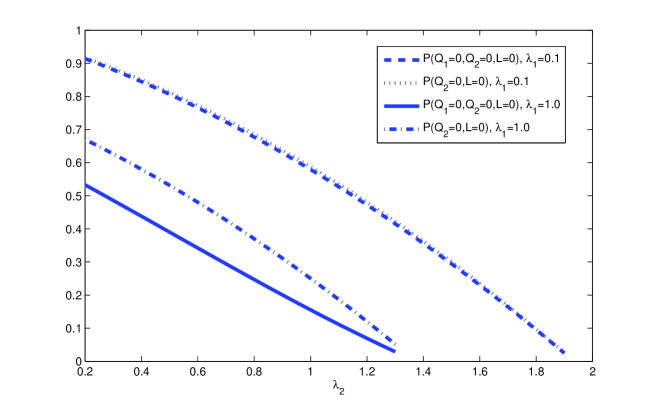
Figure 3: Probability of an empty system ($\mu=4$, $\mu_{1}=\mu_{2}=2$).

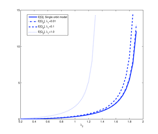
Figure 4: The expected orbit queue size, $E[Q_{2}]$ ($\mu=4$, $\mu_{1}=\mu_{2}=2$).

Next, we investigate how the retrial rates affect the system performance. Let us fix $\lambda_{1}=\lambda_{2}=1.2$, $\mu=4$, $\mu_{1}=2$ and we vary $\mu_{2}$ in the interval $[2.0;2.15]$. With such parameter setting, the system is not too far from the stability boundary. We plot in Figure 5 the expected lengths of the orbit queues, $E[Q_{1}]$ and $E[Q_{2}]$, as functions of $\mu_{2}$. We can see that if the jobs of type 2 retry at a bit faster rate than the jobs of type 1, they can gain significantly in terms of the waiting time. Specifically, an increase of less than 10% of the retrial rate of jobs of type 2 helps them to reduce the expected orbit queue length by 50%. Clearly, if there is no cost for retrials, it is beneficial for the jobs to increase their retrial rate. However, there are good reasons to keep the control of the retrial rates in the hand of the system administrator and not to set them too high. As was just mentioned, the first reason is the possible cost for retrials. The second reason is the creation of incentives to respect the contract. To illustrate this point, we fix $\lambda_{1}=1$, $\mu_{1}=\mu_{2}=2$, $\mu=4$, and vary $\lambda_{2}$ in the interval $[0.2;1.34]$. In Figure 6, we plot the expected queue lengths of the orbit queues. We see that if the jobs of type 2 increase their input rate beyond their fair share, they will be severely penalized in terms of the expected delay, whereas the increase of the input rate of jobs of type 2 does not inflict any significant damage to the jobs of type 1.

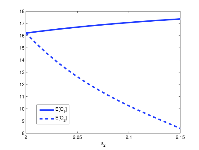
Figure 5: The expected queue lengths of the orbit queues as functions of $\mu_{2}$ ($\lambda_{1}=\lambda_{2}=1.2$, $\mu=4$, $\mu_{1}=2$).

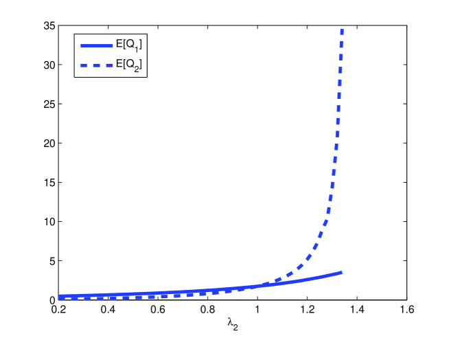
Figure 6: The expected queue lengths of the orbit queues as functions of $\lambda_{2}$ ($\lambda_{1}=1$, $\mu_{1}=\mu_{2}=2$, $\mu=4$).

Appendix A Appendix

Lemma A.1

Under conditions (32), (i) $A(k(y),y)\not=0$ and (ii) $B(k(y),y)\not=0$ for
$y\in[y_{1},y_{2}]$.

Equivalenty, (iii) $A(x,h(x))\not=0$ and (iv) $B(x,h(x))\not=0$ for $x\in C_{\sqrt{\hat{\mu}_{1}/\hat{\lambda}_{1}}}$.

Proof. From (36) and (38) we see that $R(x,y)$ and $B(x,y)$ vanish simultaneously if and only if

$$(1-x)(\lambda_{1}x-\mu)+\lambda_{2}(1-y)x = 0$$

$$\lambda(1-x)y+\mu_{2}(y-x) = 0.$$

The second equation gives $x=(\lambda+\mu_{2})y/((\lambda y+\mu_{2}))$. Plugging this value of $x$ into the first equation yields (Hint: use $\lambda=\lambda_{1}+\lambda_{2}$)

$$P_{1}(y):=(1-y)Q_{1}(y)$$

with $Q_{1}(y):=\lambda\lambda_{2}(\lambda+\mu_{2})y^{2}+(\lambda+\mu_{2}-\mu)\lambda\mu_{2}y-\mu\mu_{2}^{2}=0$.

From $\lim_{y\to\pm\infty}Q_{1}(y)=+\infty$ and $Q_{1}(0)=-\mu\mu_{2}^{2}$ we conclude that the polynomial $Q_{1}(y)$ has two real roots, $y_{-}<0<y_{+}$ and that $Q_{1}(y)<0$ for $0\leq y<y_{+}$. Since

$$Q_{1}(1)=\left(\frac{\lambda+\mu_{2}}{\mu\mu_{2}}\right)\left(\frac{\lambda}{\mu}\left(1+\frac{\lambda_{2}}{\mu_{2}}\right)-1\right)<0,$$ (77)

where the latter inequality holds under conditions (32), we conclude that $Q_{1}(y)<0$ for $y\in[0,1]$, which in turn implies that $P_{1}(y)<0$ for $y\in[0,1)$. The latter completes the proof of (ii) since $[y_{1},y_{2}]\subset[0,1)$ (see (48)).

The proof of (i) is the same as the proof of (ii) up to interchanging incides $1$ and $2$.

Eqns (iii) and (iv) both follow from the fact that $k([y_{1},y_{2}])=C_{\sqrt{\hat{\mu}_{1}/\hat{\lambda}_{1}}}$ (cf. Proposition 5.1-(11)) and the relation $h(k(y))=y$ for $y\in[y_{1},y_{2}]$ (cf. Proposition 5.1-(d1)).  

Lemma A.2

Under condition A, $h(x)$ is analytic for $1<|x|<\sqrt{\hat{\mu}_{1}/\hat{\lambda}_{1}}$ and continuous for $1\leq|x|\leq\sqrt{\hat{\mu}_{1}/\hat{\lambda}_{1}}$

Proof. We already know by Proposition 5.1 that $h(x)$ is analytic for $x\in\mathbb{C}-[x_{1},x_{2}]-[x_{3},x_{4}]$ where $x_{2}\leq 1<x_{3}$. It is therefore enough to show that $\sqrt{\hat{\mu}_{1}/\hat{\lambda}_{1}}<x_{3}$ or, equivalently from (50) that $e_{+}\left(\sqrt{\hat{\mu}_{1}/\hat{\lambda}_{1}}\right)<0$. Easy algebra shows that $e_{+}\left(\sqrt{\hat{\mu}_{1}/\hat{\lambda}_{1}}\right)=-\sqrt{\hat{\mu}_{1}/\hat{\lambda}_{1}}\left(\left(\sqrt{\hat{\lambda}_{1}}-\sqrt{\hat{\mu}_{1}}\right)^{2}+\left(\sqrt{\hat{\lambda}_{2}}+\sqrt{\hat{\mu}_{2}}\right)^{2}\right)<0$, which concludes the proof.  

Lemma A.3

Assume that conditions (32) hold. Define

$$x_{0}:=\frac{-(\lambda+\mu_{1}-\mu)\lambda\mu_{1}+\sqrt{((\lambda+\mu_{1}-\mu)\lambda\mu_{1})^{2}+4\lambda\lambda_{1}(\lambda+\mu_{1})\mu\mu_{1}^{2}}}{2\lambda\lambda_{1}(\lambda+\mu_{1})}>1$$

If $x_{0}\leq\sqrt{\hat{\mu}_{1}/\hat{\lambda}_{1}}$ and if $(\lambda+\mu_{1})x_{0}/(\lambda x_{0}+\mu_{1})\leq\sqrt{\hat{\mu}_{2}/\hat{\lambda}_{2}}$ then $A(x,h(x))$ has exactly one zero $x=x_{0}$ in $\left(1,\sqrt{\hat{\mu}_{1}/\hat{\lambda}_{1}}\right]$ and this zero has multiplicity one. Otherwise $A(x,h(x))$ has no zero in $\left(1,\sqrt{\hat{\mu}_{1}/\hat{\lambda}_{1}}\right]$.

Proof. From (35) and (37) we see that $R(x,y)$ and $A(x,y)$ vanish simultaneously if and only if

$$(1-y)(\lambda_{2}y-\mu)+\lambda_{1}(1-x)y = 0$$

$$\lambda(1-y)x+\mu_{1}(x-y) = 0.$$

The second equation gives

$$y=\frac{(\lambda+\mu_{1})x}{\lambda x+\mu_{1}}.$$ (78)

Plugging this value of $y$ into the first equation yields

$$P_{2}(x):=\frac{1-x}{(\lambda x+\mu_{1})^{2}}\,Q_{2}(x)$$

with $Q_{2}(x):=\lambda\lambda_{1}(\lambda+\mu_{1})x^{2}+(\lambda+\mu_{1}-\mu)\lambda\mu_{1}x-\mu\mu_{1}^{2}$.

The polynomial $Q_{2}(x)$ has exactly one positive zero given by $x_{0}$. From the inequality

$$Q_{2}(1)=\mu\mu_{1}(\lambda+\mu_{1})\left(\frac{\lambda}{\mu}+\frac{\lambda\lambda_{1}}{\mu\mu_{1}}-1\right)<0$$

which holds from (32), together with $\lim_{x\to\pm\infty}Q_{2}(x)=+\infty$ and $Q_{2}(0)<0$, we conclude that $1<x_{0}$.

This shows that

• If $x_{0}>\sqrt{\hat{\mu}_{1}/\hat{\lambda}_{1}}$ then $A(x,h(x))$ has no zero in $(1,\sqrt{\hat{\mu}_{1}/\hat{\lambda}_{1}}]$;

• Assume that $x_{0}\leq\sqrt{\hat{\mu}_{1}/\hat{\lambda}_{1}}$. $A(x,h(x))$ as a unique zero in $(1,\sqrt{\hat{\mu}_{1}/\hat{\lambda}_{1}}]$, given by $x=x_{0}$ provided that (see (78)) $h(x_{0})=(\lambda+\mu_{1})x_{0}/(\lambda x_{0}+\mu_{1})\leq\sqrt{\hat{\mu}_{2}/\hat{\lambda}_{2}}$ since we know from Proposition 5.1-(b2) that the branch $h(x)$ is such that $|h(x)|\leq\sqrt{\hat{\mu}_{2}/\hat{\lambda}_{2}}$ for all $x\in\mathbb{C}$; if $(\lambda+\mu_{1})x_{0}/(\lambda x_{0}+\mu_{1})>\sqrt{\hat{\mu}_{2}/\hat{\lambda}_{2}}$ then $A(x,h(x))$ does not vanish in $(1,\sqrt{\hat{\mu}_{1}/\hat{\lambda}_{1}}]$.

We are left with proving that when $A(x,h(x))$ vanishes at $x=x_{0}$ then this zero has multiplicity one. From now on we assume that $A(x_{0},h(x_{0}))=0$.

From the definition of $h(x)$ and (37) we get

$$0=R(x,h(x))=\frac{\alpha}{\mu_{2}}A(x,h(x))+\mu[\lambda(1-h(x))x+\mu_{1}(x-h(x))].$$

Differentiating this equation w.r.t. $x$ gives

$$0=\frac{\alpha}{\mu_{2}}\frac{dA(x,h(x))}{dx}+\mu[-\lambda h^{\prime}(x)x+\lambda(1-h(x))+\mu_{1}(1-h^{\prime}(x))].$$ (79)

Assume that $dA(x,h(x))/dx=0$ at point $x=x_{0}$, namely, assume that $A(x,h(x))$ has a zero of multiplicity at least two at $x=x_{0}$. From (79) this implies

$$-\lambda h^{\prime}(x_{0})x_{0}+\lambda(1-h(x_{0}))+\mu_{1}(1-h^{\prime}(x_{0})=0$$

that is

$$h^{\prime}(x_{0})=\mu_{1}\frac{\lambda+\mu_{1}}{(\lambda x_{0}+\mu_{1})^{2}}$$ (80)

with $h(x_{0})=(\lambda+\mu_{1})x_{0}/(\lambda x_{0}+\mu_{1})$ (see (78).

On the other hand, letting $(x,y)=(x,h(x))$ in (35) yields

$$A(x,h(x))=((1-h(x))(\lambda_{2}h(x)-\mu)+\lambda_{1}(1-x)h(x))\mu_{2}x.$$ (81)

Differentiating $A(x,h(x)$ wrt $x$ in (81) and letting $x=x_{0}$ gives

$$\frac{dA(x,h(x))}{dx}|_{x=x_{0}}=$$

$$[-h^{\prime}(x_{0})(\lambda h(x_{0})-\mu)+\lambda_{2}(1-h(x_{0}))h^{\prime}(x_{0})-\lambda_{1}h(x_{0})+\lambda_{1}(1-x_{0})h^{\prime}(x_{0})]\mu_{2}x_{0}$$

$$+\frac{\mu_{2}}{x_{0}}A(x_{0},h(x_{0}))$$

$$= [h^{\prime}(x_{0})(-2\lambda_{2}h(x_{0})+\lambda_{2}+\mu+\lambda_{1}(1-x_{0}))-\lambda_{1}h(x_{0})]\mu_{2}x_{0}$$

$$+\frac{\mu_{2}}{x_{0}}A(x_{0},h(x_{0}))$$

$$= [h^{\prime}(x_{0})(-2\lambda_{2}h(x_{0})+\lambda_{2}+\mu+\lambda_{1}(1-x_{0}))-\lambda_{1}h(x_{0})]\mu_{2}x_{0}$$

since $A(x_{0},h(x_{0}))=0$. Therefore, $dA(x,h(x))/dx=0$ at point $x=x_{0}$ iff (note that $x_{0}\not=0$)

$$h^{\prime}(x_{0})(-2\lambda_{2}h(x_{0})+\lambda_{2}+\mu+\lambda_{1}(1-x_{0}))-\lambda_{1}h(x_{0})=0.$$

Since $-2\lambda_{2}h(x_{0})+\lambda_{2}+\mu+\lambda_{1}(1-x_{0})<0$ because $x_{0}>1$, we get

$$h^{\prime}(x_{0})=\frac{\lambda_{1}h(x_{0})}{-2\lambda_{2}h(x_{0})+\lambda_{2}+\mu+\lambda_{1}(1-x_{0})}$$

with (see (78) $h(x_{0})=(\lambda+\mu_{1})x_{0}/(\lambda x_{0}+\mu_{1})$, so that $h^{\prime}(x_{0})<0$. However, $h^{\prime}(x_{0})>0$ in (80). This yields a contradiction, thereby implying that $dA(x,h(x))/dx$ does not vanish at point $x=x_{0}$ when $A(x,h(x))$ does or, equivalently, that $x_{0}$ is a zero of multiplicity one.  

Lemma A.4

Under conditions (32) and Assumption A the index $\chi$ of the Riemann-Hilbert problem (the index is defined in (61)) is equal to zero.

Proof.

Recall the definition of $U(x)$ in (57). First, by studying $U(\sqrt{\hat{\mu}_{1}/\hat{\lambda}_{1}}e^{i\theta})$ for $\theta\in[0,2\pi)$ it is easily seen that $U(x)$ describes a closed (and simple) contour when $x$ describes the circle $C_{\sqrt{\hat{\mu}_{1}/\hat{\lambda}_{1}}}$; moreover, for $x\in C_{\sqrt{\hat{\mu}_{1}/\hat{\lambda}_{1}}}$, $U(x)$ takes only real values when $x\in\{-\sqrt{\hat{\mu}_{1}/\hat{\lambda}_{1}},\sqrt{\hat{\mu}_{1}/\hat{\lambda}_{1}}\}$.

As a result, we will show that $\chi=0$ if we show that

$$U\left(-\sqrt{\hat{\mu}_{1}/\hat{\lambda}_{1}}\right)\times U\left(\sqrt{\hat{\mu}_{1}/\hat{\lambda}_{1}}\right)>0,$$ (82)

since (82) will imply that the contour defined by $\{U(x):|x|=\sqrt{\hat{\mu}_{1}/\hat{\lambda}_{1}}\}$ does not contain the point $x=0$ in its interior, so that by definition of the index, $\chi=0$.

We have from (37)-(38) (Hint: $R(x,h(x))=0$ by definition of $h(x))$)

$$A(x,h(x)) = -\frac{\mu\mu_{2}}{\alpha}(\lambda(1-h(x))x+\mu_{1}(x-h(x))$$ (83)

$$B(x,h(x)) = -\frac{\mu\mu_{1}}{\alpha}(\lambda(1-x)h(x)+\mu_{2}(h(x)-x)).$$ (84)

Define $x_{-}:=-\sqrt{\hat{\mu}_{1}/\hat{\lambda}_{1}}$ and $x_{+}:=\sqrt{\hat{\mu}_{1}/\hat{\lambda}_{1}}$.

By Assumption A we know that $x_{-}<-1$ and $x_{+}>1$. Also note that $h(x_{-})=y_{1}<1$ and $h(x_{+})=y_{2}<1$ from Proposition 5.1-(d2) and (48). With this, it it is easily seen from (83)-(84) that

$$A(x_{-},h(x_{-}))>0\quad\hbox{and}\quad A(x_{+},h(x_{+}))<0$$

and

$$B(x_{-},h(x_{-}))<0\quad\hbox{and}\quad B(x_{+},h(x_{+}))>0$$

so that

$$A(x_{-},h(x_{-}))/B(x_{-},h(x_{-}))<0\quad\hbox{and}\quad(A(x_{+},h(x_{+}))/B(x_{+},h(x_{+}))<0.$$

and, therefore,

$$A(x_{-},h(x_{-}))/B(x_{-},h(x_{-}))\,A(x_{+},h(x_{+}))/B(x_{+},h(x_{+}))>0.$$ (85)

The above shows that (82) is true if $r=0$ in the definition of $U(x)$ since in this case $U(x)=A(x,h(x))/B(x,h(x))$.

Assume that $r=1$ in the definition of $U(x)$ with $x_{0}<x_{+}$ and $(\lambda+\mu_{1})x_{0}/(\lambda x_{0}+\mu_{1})\leq\sqrt{\hat{\mu}_{2}/\hat{\lambda}_{2}}$. Since $(x-x_{0})<0$ for $x=x_{-}$ and $(x-x_{0})>0$ for $x=x_{+}$ we conclude from (85) that $U(x_{-})>0$ and $U(x_{+})>0$, thereby showing that (82) is also true in this case.

It remains to investigate the case when $r=1$ with $x_{0}=x_{+}$ and $(\lambda+\mu_{1})x_{0}/(\lambda x_{0}+\mu_{1})\leq\sqrt{\hat{\mu}_{2}/\hat{\lambda}_{2}}$. Clearly, $U(x_{-})>0$ since, from (85), $A(x_{-},h(x_{-}))/B(x_{-},h(x_{-}))<0$ and $(x_{-}-x_{0})<0$ because $x_{-}<-1$.

Let us focus on the sign of $U(x_{+})$. We know that the mapping $x\to U(x)$ is continuous for $|x|\leq x_{+}$ and that $U(x_{+})\not=0$ when $x_{+}=x_{0}$. Since we have shown that $U(x_{+})>0$ when $x_{0}<x_{+}$ and $(\lambda+\mu_{1})x_{0}/(\lambda x_{0}+\mu_{1})\leq\sqrt{\hat{\mu}_{2}/\hat{\lambda}_{2}}$, we deduce, by continuity, that necessarily $U(x_{+})>0$ when $x_{+}=x_{0}$ and $(\lambda+\mu_{1})x_{0}/(\lambda x_{0}+\mu_{1})\leq\sqrt{\hat{\mu}_{2}/\hat{\lambda}_{2}}$, which concludes the proof.  

Lemma A.5

Under condition (32) and Assumption A, $B(k(y),y)=0$ for $|y|=1$, $y\not=1$. Also, $B(k(y),y)$ has a zero at $y=1$, with multiplicity one.

Proof. Fix $|y|=1$, $y\not=1$. We know from Proposition 5.1-(a1) that $|k(y)|<1$.

From (38) and the fact that $R(k(y),y)=0$ by definition of $k(y)$, we see that $B(k(y),y)=0$ is equivalent to

$$0=\lambda(1-k(y))y+\mu_{2}(y-k(y))=(\lambda(1-k(y))+\mu_{2})y-\mu_{2}k(y)$$

that is,

$$\lambda(1-k(y)+\mu_{2})y=\mu_{2}k(y).$$

Taking the absolute value in both sides of the above equation yields

$$|\lambda(1-k(y)+\mu_{2})|=|\lambda(1-k(y)+\mu_{2})y|=|\mu_{2}k(y)|<\mu_{2}.$$ (86)

But $|\lambda(1-k(y))+\mu_{2})|>\mu_{2}$ which contradicts (86). Hence, $B(k(y),y)\not=0$ for $|y|=1$, $y\not=1$.

Since $k(1)=1$, we see that $B(k(1),1)=B(1,1)=0$ from the definition of $B(x,y)$. Let us show that the multiplicity of this zero is one. This amounts to showing that $dB(k(y),y)/dy$ does not vanish at $y=1$.

Differentiating $B(k(y),y)$ w.r.t. $y$ in (38) (Hint: $R(k(y),y)=0$) and setting $y=1$, gives

$$\frac{dB(k(y),y)}{dy}|_{y=1}=\frac{\mu\mu_{1}}{\alpha}((\lambda+\mu_{2})k^{\prime}(1)-\mu_{2}).$$ (87)

Let us calculate $k^{\prime}(1)$, the derivative of $k(y)$ at $y=1$. To this end, let us use (34) to differentiate $R(k(y),y)$ (which is equal to zero) w.r.t. $y$, which gives

$$0=\frac{dR(k(y),y)}{dy}|_{y=1}=(\mu\mu_{1}-\alpha\lambda_{1})k^{\prime}(1)+\mu\mu_{2}-\alpha\lambda_{2}$$ (88)

so that $k^{\prime}(1)=(\alpha\lambda_{2}-\mu\mu_{2})/(\mu\mu_{1}-\alpha\lambda_{1})$ (note that $\mu\mu_{1}-\alpha\lambda_{1}\not=0$ from Assumption A, which shows that $k^{\prime}(1)$ is well defined). Plugging this value of $k^{\prime}(1)$ into (87) gives

$$\frac{dB(k(y),y)}{dy}|_{y=1} = \frac{\mu\mu_{1}}{\alpha(\mu\mu_{1}-\alpha\lambda_{1})}\,((\alpha\lambda_{2}-\mu\mu_{2})(\lambda+\mu_{2})-\mu_{2}(\mu\mu_{1}-\alpha\lambda_{1}))$$

$$= \frac{\mu\mu_{1}}{\alpha(\mu\mu_{1}-\alpha\lambda_{1})}\alpha(\lambda\lambda_{2}+\lambda\mu_{2}-\mu\mu_{2})$$

$$= \frac{\mu\mu_{1}}{\mu\mu_{1}-\alpha\lambda_{1}}\mu\mu_{2}\left(\frac{\lambda\lambda_{2}}{\mu\mu_{2}}+\frac{\lambda}{\mu}-1\right)<0$$

under the conditions in (32) (to establish the 2nd equality we have used the definitions of $\alpha$ and $\lambda$). This proves that $dB(k(y),y)/dy|_{y=1}\not=0$ and completes the proof.

References

[1] J. R. Artalejo, “Accessible bibliography on retrial queues”.
Math. and Comp. Modeling. 30, 223-233 (1999).
[2] J. R. Artalejo and A. Gómez-Corral,
Retrial Queueing Systems: A Computational Approach. Springer, Berlin (2008).
[3] J. R. Artalejo, A. Gómez-Corral and M. F. Neuts,
“Analysis of multiserver queues with constant retrial rate”.
European Journal of Operational Research. 135, 569-581 (2001).
[4] K. Avrachenkov and U. Yechiali,
“Retrial networks with finite buffers and their application to internet data traffic”.
Prob. Eng. Inf. Sci. 22, 519-536 (2008).
[5] K. Avrachenkov and U. Yechiali,
“On tandem blocking queues with a common retrial queue”. Comp. Oper. Research.
37, 1174-1180 (2010).
[6]
K. Avrachenkov and E. Morozov, “Stability analysis of GI/G/c/K retrial queue with
constant retrial rate”. Inria Research Report no. 7335 (2010).
[7] K. Avrachenkov, E. Morozov, R. Nekrasova and B. Steyaert,
“On the stability and simulation of a retrial system with constant retrial rate”.
in Proceedings of the 9th International Workshop on Retrial Queues, June 2012.
[8] D. Bertsekas and R. Gallager, Data Networks. 2nd ed., Prentice-Hall
International (1992).
[9]
J. P. C. Blanc, “Asymptotic analysis of a queueing system with a two-dimensional state space”.
J. Appl. Prob. 21, 870-886 (1984).
[10]
J. P. C. Blanc, R. Iasnogorodski and P. Nain, “Analysis of the M/GI/1 ./M/1 queueing model”.
Queueing Systems. 3, 129-156 (1988).
[11] P. P. Bocharov, C. D’Apice, A. V. Pechinkin and S. Salerno,
Queueing Theory. Modern Probability and Statistics Series, VSP, Utrecht (2004).
[12] J. Brandon and U. Yechiali,
“A tandem Jackson network with feedback to the first node”. Queueing Systems.
9, 337-352 (1991).
[13] B. D. Choi, K. K. Park and C. E. M. Pearce, “An M/M/1 retrial queue with control policy
and general retrial times”. Queueing Systems. 14, 275-292 (1993).
[14] B. D. Choi, K. H. Rhee and K. K. Park, “The M/G/1 retrial queue with retrial rate control
policy”. Prob. Eng. Inf. Sci. 7, 29-46 (1993).
[15] J. W. Cohen and O. J. Boxma, Boundary Value Problems in Queueing System Analysis.
North Holland, Amsterdam (1983).
[16] G. I. Falin and J. G. C. Tempelton, Retrial Queues. CRS Press, Boca Raton (1997).
[17] G. Fayolle, “A simple telephone exchange with delayed feedback”.
in Teletraffic Analysis and Computer Performance Evaluation, O.J. Boxma, J.W. Cohen, H.C. Tijms (Eds.),
Elsevier North-Holland (1986).
[18]
G. Fayolle and R. Iasnogorodski, “Two coupled processors: The reduction to a Riemann-Hilbert problem”.
Z. Wahrscheinlichkeitstheorie verw. Gebiete. 47, 325-351 (1979).
[19]
G. Fayolle, R. Iasnogorodski and I.Mitrani, “The distribution of sojourn times in a queueing network with overtaking:
Reduction to a boundary problem”.
Proc. Performance 1983, A. K. Agrawala and S. K. Tripathi Eds., College Park, MD, May 25-27, 477-486 (1983).
[20]
G. Fayolle, P. J. B. King and I. Mitrani, “The solution of certain two-dimensional Markov models”.
Adv. Appl. Prob. 14, 295-308 (1982).
[21]
F. D. Ghakov, Boundary Value Problems. Pergamon Press, Oxford (1961).
[22]
N. I. Mushkelishvili, Singular Integral Equations. Noordhoff, Groningen (1953).
[23]
P. Nain, “Analysis of a two-node Aloha network with infinite capacity buffers”. Proc.
Int. Seminar on Computer Networking and Performance Evaluation, T. Hasegawa, H. Takagi and
Y. Takahashi, Eds., Tokyo, Japan, Sep. 18-20 (1985).
[24]
W. Szpankowski, “Stability conditions for some multiqueue distributed systems:
Buffered random access systems”.
Adv. in Applied Prob. 26, 498-515 (1994).
[25] U. Yechiali, “Sequencing an N-stage process with feedback”.
Prob. Eng. Inf. Sci. 2, 263-265 (1988).